Review

Monitoring Groundwater Storage Changes Using the Gravity Recovery and Climate Experiment (GRACE) Satellite Mission: A Review

by
Frédéric Frappart
1,2,* and
Guillaume Ramillien
1
1
Géosciences Environnement Toulouse (GET), UMR 5563, CNRS/IRD/UPS, Observatoire Midi-Pyrénées 8 (OMP), 14 Avenue Edouard Belin, 31400 Toulouse, France
2
Laboratoire d’etudes en Géophysique et Océanographie Spatiales (LEGOS), UMR 5566, CNRS/IRD/UPS, Observatoire Midi-Pyrénées 8 (OMP), 14 Avenue Edouard Belin, 31400 Toulouse, France
*
Author to whom correspondence should be addressed.
Remote Sens. 2018, 10(6), 829; https://doi.org/10.3390/rs10060829
Submission received: 1 March 2018 / Revised: 10 May 2018 / Accepted: 17 May 2018 / Published: 25 May 2018
(This article belongs to the Special Issue Remote Sensing of Groundwater from River Basin to Global Scales)

Abstract

:
The Gravity Recovery and Climate Experiment (GRACE) satellite mission, which was in operation from March 2002 to June 2017, was the first remote sensing mission to provide temporal variations of Terrestrial Water Storage (TWS), which is the sum of the water masses that were contained in the soil column (i.e., snow, surface water, soil moisture, and groundwater), at a spatial resolution of a few hundred kilometers. As in situ level measurements are generally not sufficiently available for monitoring groundwater changes at the regional-scale, this unique dataset, combined with external information, is widely used to quantify the interannual variations of groundwater storage in the world’s major aquifers. GRACE-based groundwater changes revealed significant aquifer depletion over large regions, such as the Middle East, the northwest India aquifer, the North China Plain aquifer, the Murray-Darling Basin in Australia, the High Plains, and the California Central Valley aquifers in the United States of America (USA), but were also used to estimate groundwater-related parameters such as the specific yield, which relates groundwater level to storage, or to define the indices of groundwater depletion and stress. In this review, the approaches used for estimating groundwater storage variations are presented along with the main applications of GRACE data for groundwater monitoring. Issues that were related to the use of GRACE-based TWS are also addressed.

1. Introduction

Globally, water volume stored in the aquifers is estimated to be about 23.4 × 10⁶ km3, i.e., around half of the fresh water that is only about 2.5% of the total water present on Earth [1]. Aquifer systems play an important role in the global hydrological and the biogeochemical cycles and ecosystems sustainability [2,3,4,5]. Groundwater is a key resource supplying water to billions of people and sustaining agricultural, industrial, and domestic activities [6,7]. It is often the last fresh water resource available for supplying water for domestic use and irrigation after the depletion of surface water in semi-arid areas and densely populated countries [7].
The development of groundwater use has led to depleted levels in many regions around the world [8,9,10]. A global groundwater depletion of 4500 km3 (or 41.4 km3·year−1) was estimated between 1900 and 2008 [11], which represents a major threat to global water security, thus potentially causing a decline in agricultural productivity and energy production. It might also result in conflicts around the world [12]. In the Unites States (US) alone, the groundwater depletion was estimated to be of 1000 km3 (9.2 km3·year−1), with an increase since 1950, and a maximum depletion rate of 24 km3·year−1, observed since 2000 [13]. Globally, the groundwater depletion rate increased from 126 ± 32 km3·year−1 to 283 ± 40 km3·year−1 between 1960 and 2000. In 2000, groundwater depletion reached 39 ± 10% of the global yearly groundwater abstraction [10]. This increase in groundwater use is attributed to growth of the population and an increase of the economic activity, e.g., expansion of the irrigated areas. According to Zekster et al. [14], 20% of the global withdrawals for irrigation, 40% of the total withdrawals for industrial activities, and 50% of the total withdrawals by municipalities come from the groundwater. Total groundwater withdrawals range from 600 to 1100 km3·year−1 (i.e., one-fifth to one third of the total global freshwater abstraction) [14,15,16]. The consumption of groundwater for irrigation is estimated to be 545 km3·year−1 (43% of the total water used for irrigation) [7]. Groundwater depletion (i.e., groundwater abstraction exceeds groundwater recharge), which occurs over a long time-period and extensive areas, has significant impacts on natural streamflow, groundwater level, and, as a consequence, even on land subsidence and salt water intrusion in deltaic areas, in turn, causing the degradation of ecosystems and the deterioration of groundwater quality [10,17]. Globally, groundwater is currently overexploited: its footprint exceeds the actual aquifers area by about 3.5 times. About 1.7 billion of the world’s population lives in areas where groundwater resources are under stress [9].
Climate change is expected to have substantial direct impacts on groundwater water recharge, and hence, on renewable groundwater resources and indirect ones through changes in groundwater use [16,18,19]. Direct impacts relate to climate effects on other reservoirs (droughts and floods intensity and duration in the surface reservoir for instance) and fluxes (rain and snow falls an evapotranspiration) and on land cover. Indirect effects are related to human activity, e.g., expansion of rain-fed and irrigated agriculture [19]. Numerical simulations that were based on climate change scenarios, and taking population density into account, revealed that between 15% and 20% of the world population will be affected by groundwater decreases by the year 2050 [16].
In this context, long-term reliable, compact and frequent observations of the aquifer levels are necessary to monitor groundwater storage and its changes over time. The launch of the Gravity Recovery and Climate Experiment (GRACE) mission in March 2002 offered new perspectives for the monitoring of terrestrial part of the hydrological cycle, including groundwater resources [20]. The GRACE mission measures the tiny variations in the Earth gravity field that are related to changes in Terrestrial Water Storage (TWS) [20,21]. Anomalies of TWS from GRACE are commonly used in hydrological applications from regional to global scales (see [22,23] for recent reviews). Alone or in combination with external datasets, the GRACE data provide a new source of information on extreme climatic events, such as exceptional droughts and floods [24,25,26], on snow accumulation [27], and on basin-scale hydrological fluxes, such as fresh water discharge [28,29] or evapotranspiration [30,31].
Using in situ aquifer level measurements from the High Plains aquifer, Central US, and land surface model outputs, [32] identified the potential of the GRACE mission to detect changes in groundwater (GW) storage using the GRACE data. In their study, they show that the annual amplitude of the GW changes from in situ measurements was higher than the difference between the GRACE-based TWS and the soil moisture (SM) from a land surface model, taking into account the expected accuracy of GRACE and the uncertainty on the model outputs.
In this review, the GRACE mission is described, i.e., on-board instruments, orbital characteristics, and products that were made available to the scientific community. The different approaches that were used to estimate GW changes from GRACE-based TWS are described. Next, the error budget and the validation of the GW storage changes that were estimated using the GRACE data are presented. The main results and main scientific applications are subsequently summarized. The discussion section will present the current limitations of the GRACE-derived GW changes, and which improvements can be expected with the future launches of the GRACE Follow-On (GRACE FO) and the Surface Water and Ocean Topography (SWOT) missions in 2018 and 2021, respectively.

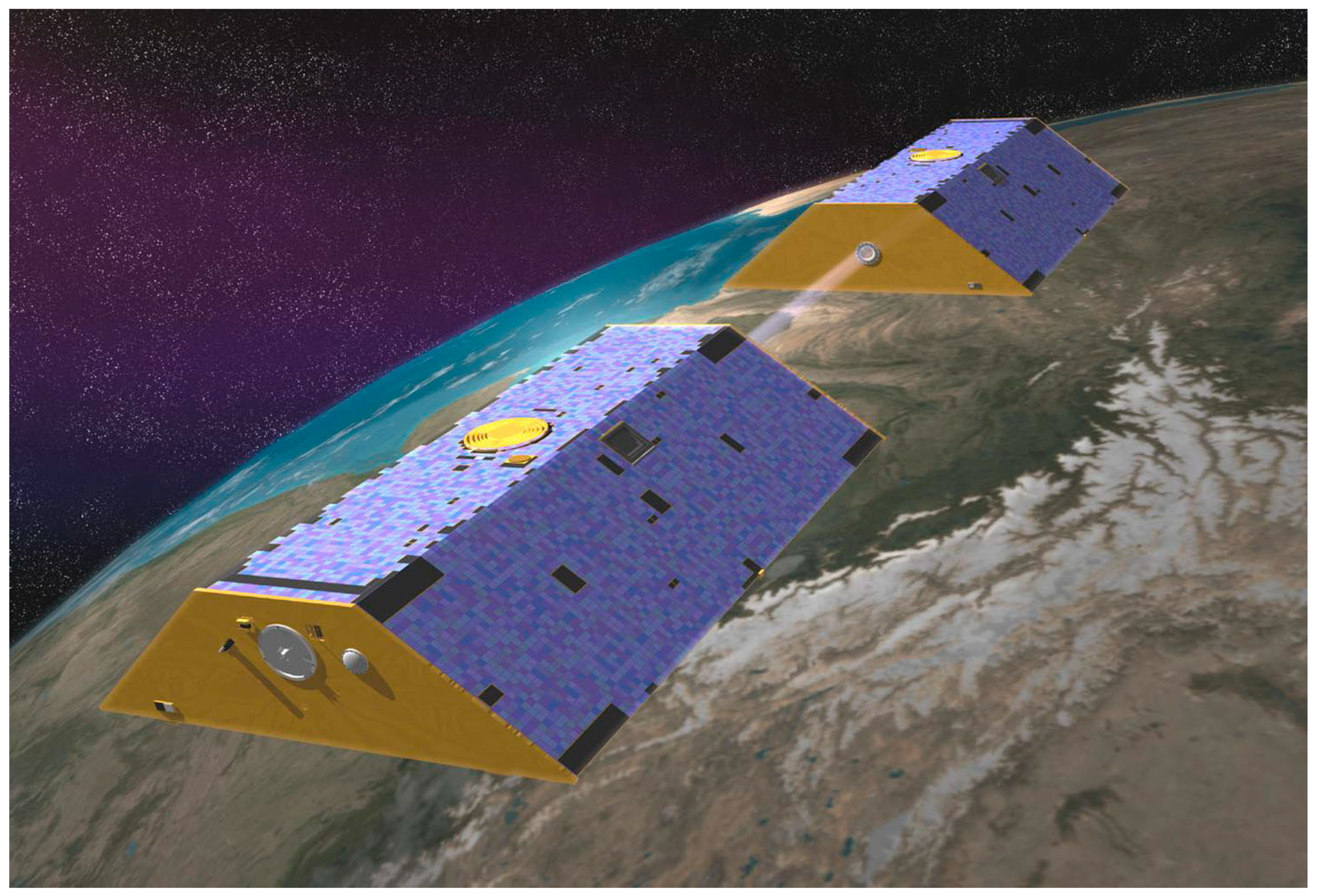
2. The GRACE Mission

2.1. Orbit and On-Board Instruments

The GRACE satellite gravity mission was jointly launched in 17 March 2002 by the American National Aeronautics and Space Administration (NASA) and the German Aerospace Center (Deutsches Zentrum für Luft- und Raumfahrt-DLR). Its scientific mission ended on 27 October 2017. The GRACE mission consists of two co-orbital satellites, which were orbiting at a relatively low average altitude of around 450 km with an inclination of 89.5°. GRACE was unique among all of the the Earth observation satellite missions, since it was composed of two vehicles that followed each other at a distance of about 220 km (Figure 1). The instantaneous measurement of distance and relative speed between the two satellites was performed by a radar telemeter operating at K-band (K-Band microwave Ranging or KBR) with a great accuracy of 1 μm·s−1 [21]. The inter-satellite distance is a function of the differences in gravitational acceleration that was experienced by each GRACE satellite [33]. The payload of each satellite was also composed of a three-axis accelerometer that provides information on the dynamic effects, including non-dissipative or conservative forces, mainly meaning solar and Earth radiation pressure, and atmospheric drag. After removing the non-gravitational effects, variations in distance and inter-satellite distance changing rate were used to estimate variations in the geopotential along the track of the twin satellites. Variations in the Earth’s gravity related to density heterogeneities and topography are reflected in changes in the observed inter-satellite distances along the orbit (Figure 2).
The payload was composed of five instruments on board each satellite component of the GRACE mission [21]:
  • the K-band ranging (KBR) system, which provides distance measurements between the two satellites, with an accuracy of 10 μm, using the phases of carrier electromagnetic waves in the K and the Ka bands, at frequencies of 26 and 32 GHz;
  • the Ultra-Stable Oscillator (USO), which generates electromagnetic waves in the K-band for the KBR system at the desired frequency;
  • the SuperSTAR accelerometers (ACC) accurately measures the non-conservative forces applied to each satellite along three axes;
  • the Stellar Camera ASSEMBLY (SCA) determines the orientation of the satellite relatively to the position of fixed stars; and,
  • The Black-Jack GPS receivers and Instrument Processing Unit provides the three components of the position and velocity of each of the satellites.
GRACE was the first mission to use the principle of two co-orbital satellites in pursuit, as proposed by [35], allowing for estimating the spatial and temporal variations of the gravitational field (i.e., the geoid), which reflect mass changes in the Earth system over time scales ranging from months to a decade [20]. The GRACE mission that was measured the sum of the effects of all the changes in mass, which were integrated along the vertical axis, of the solid Earth and of redistributions of mass within the superficial fluid envelopes [20].

2.2. Data from the GRACE Mission

Three official processing centers that form the GRACE Science Data Center (SDS) produce the level 1 products and level 2 solutions derived from measurements of the GRACE mission. They are:
  • the Center for Space Research (CSR) in Austin, Texas, United States,
  • the GeoForschungs Zentrum (GFZ) in Potsdam, Germany, and
  • the Jet Propulsion Laboratory (JPL) in Pasadena, California, United States.
Level 1b products consist of already processed positions and velocities that were measured by the on-board GPS, accelerometers, and the accurate K-band measurements of variations in distance between the two vehicles. These measurements are used to compute the monthly gravity field models or level 2 products that were expressed in geoid height or in terms of Equivalent Water Height (EWH, e.g., [36]). These products are made available by the GFZ’s Integrated System Data Center (ISDC—[37]) and JPL’s Physical Oceanography Distributive Active Data Center (PODAAC—[38]).
Other level 2 GRACE solutions can also be obtained by other research groups who might use different approaches at temporal resolutions from one day to one month in the form of spherical harmonic coefficients (global approaches) or spatial grids (local or regional approaches).
The level 2 GRACE products are obtained using a dynamic approach that is based on the Newtonian formulation of the satellite’s equation of motion in an inertial frame, with the Earth’s center as origin, combined with a dedicated modeling of gravitational and non-conservative forces acting on the spacecraft [33]. During the process, the known gravitational effects (changes in atmosphere and oceans masses, pole movement, and tides) are removed from observations using a priori information from meteorological and global ocean circulation models, as well as the non-gravitational forces that were measured by the on-board accelerometers [40,41]. The residual values that form GRACE Stokes coefficients represent, over land, represent the sum of the solid Earth contribution, the continental water storage, the errors from the correcting models, and the noise. More detailed on the phasical processed reflected in GRACE time-variable data can be found in [42]. These Stokes coefficients are first centered to suppress the contribution of the solid Earth, either removing their average that was computed over a period of several or the coefficients from a static geoid model and then converted into equivalent water storage. This processing is described in [36,42].

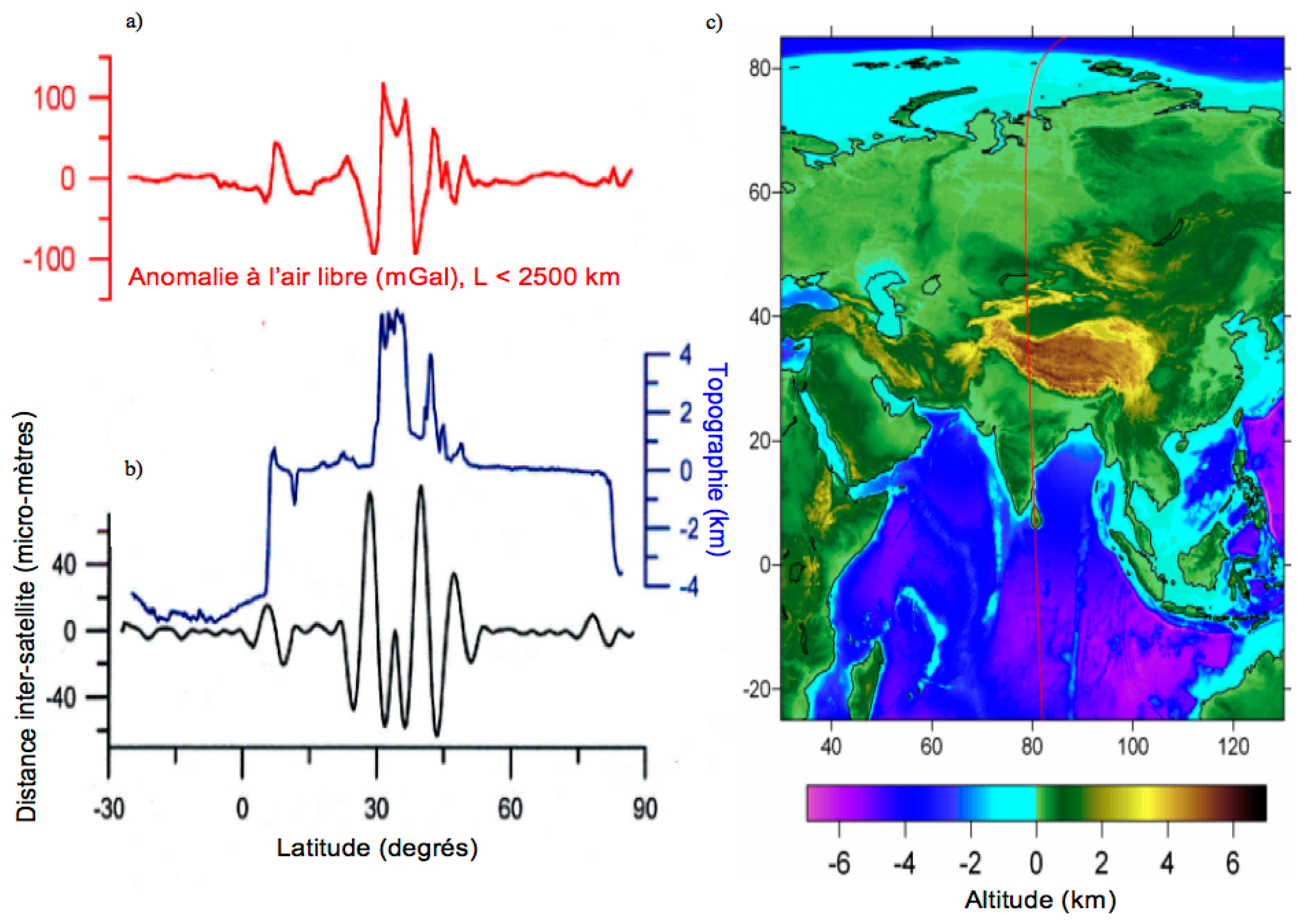
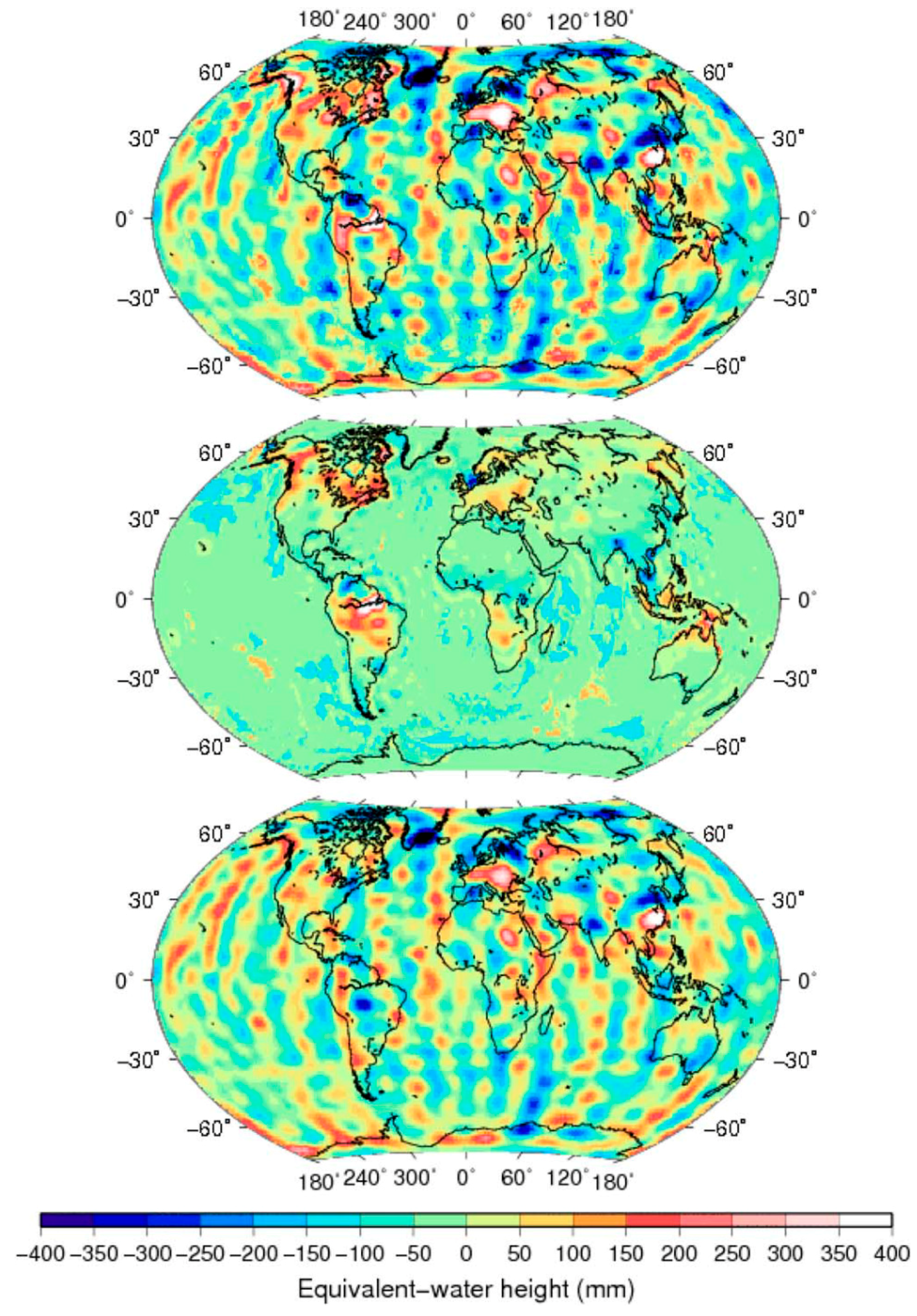
2.3. Accuracy and Spatial Resolution of GRACE-Based Products over Land

The GRACE mission provided novel information for continental hydrology research: the terrestrial water storage or integrated water content (i.e., the sum of the water contained in the soil column from the following hydrological reservoir: surface water, soil water, groundwater, snow). An early study showed an expected measurement accuracy of a few millimeters of equivalent water height (EWH), in terms of mass surface density (and for a reference water density of 1000 kg.m−3), over areas of 400 km by 400 km, which was based on Land Surface Model (LSM) outputs. The TWS retrieval was expected to be affected by the presence of noise in the shorter wavelengths [36]. In addition, spectral truncation errors increase as the area decreases. Based on LSM outputs and the expected accuracy of the GRACE land water solutions, it was estimated that the changes in TWS could be detected if they exceed 1.5 cm of EWH over an area of 200,000 km2 [43]. The accuracy of the GRACE land water solutions was expected to be around 0.7 cm EWH for a drainage area of 400,000 km2 and 0.3 cm for a drainage area of 4,000,000 km2 [44]. Current GRACE products have a spatial resolution of a few hundred kilometers (around 200 km for the Mascons and the regional solutions and 330 km for the releases 03 to 05 for a typical degree of truncation of 60). Errors were estimated to be around 40 mm at the Equator, and decreasing to 15 mm in polar regions [45].

3. Estimating Groundwater Storage Using the GRACE Data: Different Approaches

3.1. The Direct Approach

This straightforward technique consists of removing to the GRACE-based anomaly of TWS (ΔTWS) the contributions of the different hydrological reservoirs, i.e., surface (ΔWSurface water) and soil (ΔWSoil water) waters, snow (ΔWSnow) and groundwater (ΔWGroundwater):
ΔTWS = ΔWSurface water + ΔWSoil water + ΔWSnow + ΔWGroundwater
Equation (1) hence becomes:
ΔWGroundwater = ΔTWS − ΔWSurface water − ΔWSoil water − ΔWSnow
The contributions from the individual hydrological reservoirs are obtained from external sources, e.g., hydrological model outputs, in-situ data, or other remotely sensed observations. Figure 3 presents an example of terrestrial trends that were estimated over 2004–2010 from TWS from GRACE with and without the Glacial Isostatic Adjustement (GIA) correction from [46] applied, SM and snow from Global Land Data Assimilation System—National Centers for Environmental Prediction (NCEP), Oregon State University (Department of Atmospheric Sciences), Air Force, Hydrology Lab (GLDAS-NOAH), and the difference between TWS from GRACE corrected from GIA and SM and snow. GIA is the response of the solid Earth to the changes in surface loads due to the melting of large-scale ice sheets and glaciers since the last glacial maximum that occurred ~21,000 years [47]. Over land, the adjustment of the Earth surface to changing loads causes vertical uplifts with the largest trends over Fennoscandia, Northern America, Patagonia, Greenland, and Antarctica. Vertical uplift rates of ~10 mm·year−1 were recorded in Fennoscandia and near the Hudson Bay [47,48].
Several combinations to solve (2) using in situ records, model outputs, and remotely sensed observations are detailed below for a wide range of hydro-climatic conditions.

3.1.1. Regions Where TWS Is Limited to Soil Water Storage

The simplest cases relate to arid and semi-arid environments or in areas where surface waters are negligible and snow inexistent. If a dense soil moisture network exists in areas that are larger than several hundred square kilometers as Illinois or the region of the High Plains aquifer in the United States of America (USA), providing information on the water contained in the soil at several depths, groundwater storage changes can be inferred removing the anomaly of soil water content to the anomaly of TWS that was derived from GRACE [49,50,51]. Most of the times, such networks do not exist. Therefore, hydrological model or land surface model outputs are used instead, such as the ones from GLDAS [52], the WaterGAP Global Hydrology Model (WGHM) [53], and the World-Wide Water Resources Assessment (W3RA) model [54], for instance, for the High Plains aquifer [55], for the Canning aquifer in northwest Australia [56], and within the Middle East [57].

3.1.2. More Complex Environments

In more complex environments, water storage anomalies from the other hydrological reservoirs need to be taken into account using in situ data, hydrological model outputs, or remotely sensed observations, especially when surface water reservoir cannot be neglected. In-situ data were used, in combination with GLDAS outputs for SM, for monitoring the GW changes in the semi-arid Murray Darling Basin, Australia, where all SW is composed of reservoirs, lakes, weirs, and in-channel storage [58], as well as the prone to flood Bengal Basin in Bangladesh [59]. Additional information on snow from models was also taken into account to estimate GW anomalies in California Central Valley, USA [60], and in the Great Lakes Water Basin in Canada and USA [61]. Due to the lack of available in-situ data in remote and complex environments, GW retrievals from GRACE and outputs from hydrological models were performed using; for instance, GLDAS over northern India [62,63] or WGHM in the Niger and the Murray Darling Basins [64,65]. Remote sensing data were also used to provide information on the surface reservoir. Radar altimetry or radar altimetry, coupled with satellite images, was used to remove SW storage variations of lakes to TWS in lakes water basin, such as the East African Lakes [66,67] or the American Great Lakes [61], and in large aquifer regions comprising lakes and reservoirs, such as the Middle East [68,69]. In large drainage basins that were covered with extensive floodplains, surface water storage, which was obtained from the combination of altimetry-based water levels with inundation extent from satellite images, were removed from TWS to retrieve GW changes. This method was applied in the Negro River Basin, which is one of the largest tributary of the Amazon [70], and in the Lower Ob’ Basin in Siberia [71]. In this latter case, the snow storage was also derived from the GRACE data using an inverse approach [72,73].

3.2. Calibration and/or Assimilation into Hydological Models

GRACE data were also incorporated into groundwater, hydrological, and land surface models to improve the simulations of the terrestrial water cycle, including groundwater storage through calibration and data assimilation processes from regional to global scales. Due to the lack of in situ measurements of aquifer levels, hydrological models are imperfect in representing the characteristics of the groundwater changes, which is due to uncertainties of model parameters, limitations in the structure of these models, and uncertainty of input (forcing) data [74]. In spite of the coarse resolution of the GRACE Level-2 products (around 300 km but often re-sampled at 1° or 0.5°), the GRACE-based spatial pattern of GW and associated monthly temporal variations are included in the tuning process of groundwater, hydrological, and land surface models alone or as an additional regularization mechanism. GRACE data were used to constrain the hydraulic head to determine the best values for the model parameters, such as the hydraulic conductivity. Several calibration approaches were applied in various environments—an evolutionary multiobjective optimization on the regional groundwater model that was based on MODFLOW for the Edwards–Trinity Plateau and Pecos Valley aquifers, in Texas, USA [74], two meta-heuristic algorithms (particle swarm optimization and pattern search) on a groundwater flow model for the Ghaen aquifer, Iran [75], Monte-Carlo technique on a large-scale groundwater model that was based on FEFLOW is constructed for the Qaidam Basin, China [76]. These studies demonstrated that the supplementary constrain on storage changes only provided by the GRACE data highly reduced the uncertainty of the model outputs. Calibration and data assimilation of GRACE data were also performed in large-scale hydrological models. A Pareto-based multi-objective calibration approach was applied to WGHM using the GRACE-derived TWS in 28 large drainage basins. If no comparison was performed against in situ data, the calibration resulted in a decrease of the variability of groundwater storage variations at global-scale [77].
The GRACE-based TWS were also assimilated in WGHM through an ensemble-based Kalman filter approach in the Mississippi Basin. Uncertainties in the groundwater model outputs are reduced after one year of simulation, even if they remain large in the region of the High Plains aquifer due to extensive irrigation and groundwater abstraction that are poorly described in the model [78]. Incorporation GRACE-based TWS into land surface models also improved hydrological parameters and fluxes. The calibration of the Community Land Model (CLM) 3.0 [79], coupled with an unconfined aquifer model [80] with a multi-objective approach based on Monte-Carlo simulation framework using TWS from GRACE and base-flow data, improved the simulation of the water table depth. This approach, tested in Illinois, USA, is likely to be extended worldwide [81]. Assimilation of GRACE-based TWS in the Catchment Land Surface Model (CLSM) [82] using an ensemble Kalman smoother method allowed better modeling of groundwater storage variations in the Mississippi River Basin and in 18 river basins in western and central Europe [83,84]. The impact of GRACE error correlation structure on the assimilation of GRACE data was very recently studied by [85,86]. Their results indicate that incorporating GRACE data’s full covariance matrices results in more realistic groundwater estimations. Recently, Khaki et al. [86,87] applied GRACE data, through various extensions of assimilation filters and applying covariance localization, and [88] used GRACE and soil moisture data simultaneously in an ensemble-based assimilation framework to update storage estimation of a hydrological model in Australia, while [57,89] assimilate GRACE data into W3RA to estimate the groundwater changes in Bangladesh and the Middle East, respectively.

4. Error Budget and Validation of the GRACE-Based Groundwater Storage

4.1. Error Budget of the GRACE-Based Groundwater Storage

Using Equation (2), the error on GW storage variations (σGroundwater) can be written as:
σ Groundwater = ( σ TWS ) 2 + ( σ Surface   water ) 2 + ( σ Soil   water ) 2 + ( σ Snow ) 2
where σTWS, σSurface water, σSoil water, and σSnow represent the error on the TWS, surface water, soil water, and snow components, respectively.
Or similarly, on the trend:
σ aGroundwater = ( σ aTWS ) 2 + ( σ aSurface   water ) 2 + ( σ aSoil   water ) 2 + ( σ aSnow ) 2
where σaTWS, σaSurface water, σaSoil water, and σaSnow represent the one-sigma trend error on the TWS, surface water, soil water, and snow components, respectively.
Errors of GRACE data are originated from measurements, spatial and spectral leakages, post-processing, and glacial isostatic adjustment (GIA) in areas where this phenomenon is significant. Errors on trend estimates of the GRACE-based GW storage were found to be equal to 5.3 mm·year−1 for a trend of −55.9 mm·year−1 from April 2006 to March 2010 in the California Central Valley aquifer [92], of 0.3 cm·year−1 for a trend of −2.2 cm·year−1 from 2003 to 2010 in the north of China [93], 0.4  km3·year−1 for a trend of −5.6  km3·year−1 from December 2004 to November 2013 in the Colorado Basin [94], or 0.6 mm·year−1 for a trend of −27.2 mm·year−1 from 2003 to 2009 in the Tigris and the Euphrates Basin [68], when computing the error budget presented in Equation (4).

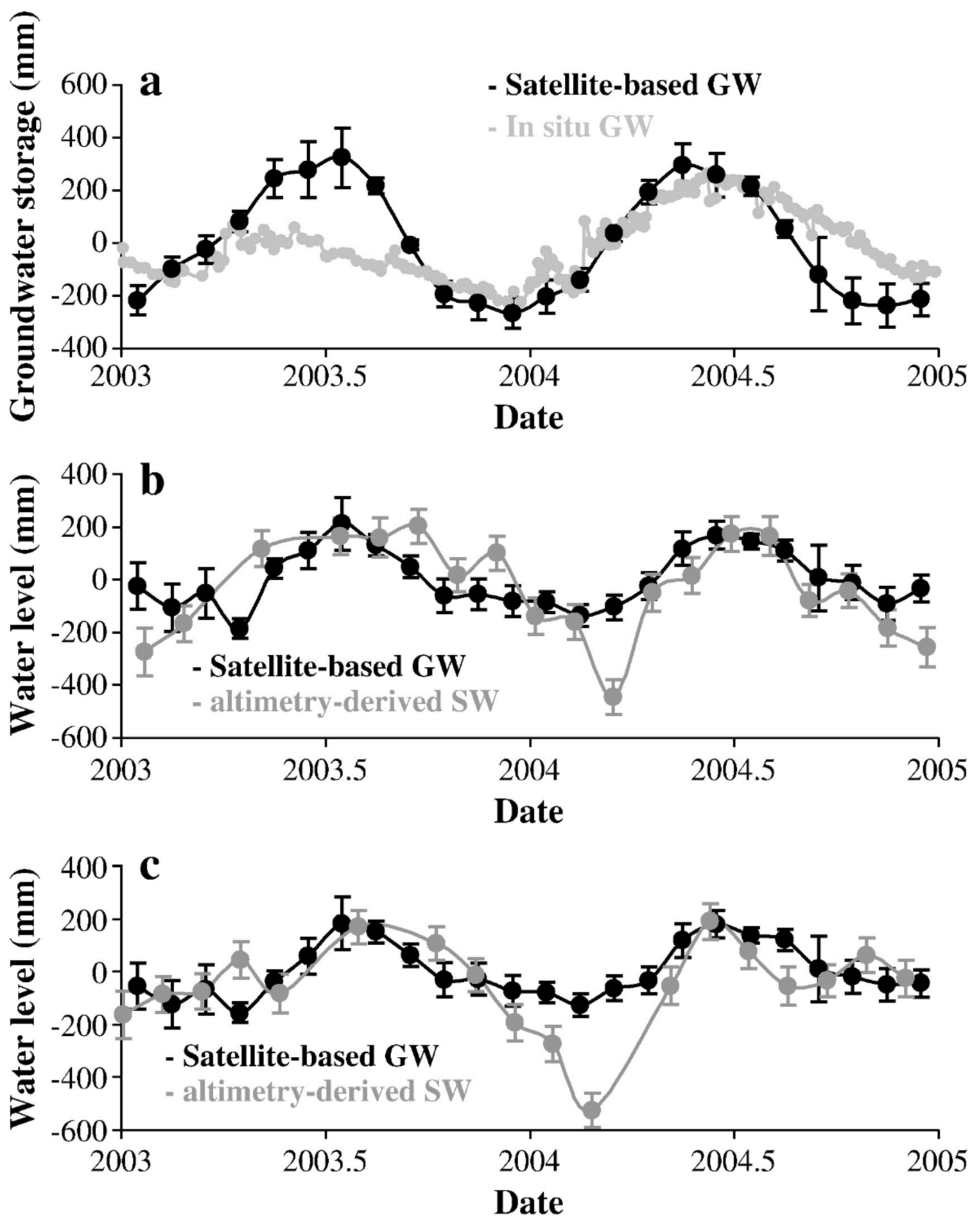
4.2. Validation of the GRACE-Based Groundwater Storage Variations

Validation of the GRACE-based GW storage was performed against in situ well measurements when available. Two different approaches were used: the validation of GRACE-based TWS comparing them to the sum of the soil moisture storage (from in-situ data or from model outputs) to the groundwater storage (from wells) or the direct validation of the GRACE-based groundwater storage anomalies that were obtained using Equation (2) against the well records. These approaches required two preliminary steps. The well depths (h) are proportional to groundwater storage through the specific yield (Sy):
WGroundwater = Sy h
Once the conversion is performed, in situ SM and GW storages are either interpolated or are averaged to be compared with GRACE-based TWS or GW storage.
The first approach was applied in Illinois using 16 wells and 16 soil moisture stations from August 2002 to November 2005 on area of 200,000 km2 [49], and 16 wells and 19 soil moisture stations from February 2003 to December 2005 on area of 280,000 km2 [95] using the GRACE Release-03 data from CSR. Very similar results were found (R = 0.83 in the first study and R = 0.95 and RMSE = 20.3 mm in the second study). The differences that were observed between these two studies can be attributed to difference in observation period, validation datasets, extent of the study area, and data processing (SM were considered to 2 and 1 m depths, respectively). The better results that were obtained are more likely to be accounted by the choice of the period (first GRACE data from 2002 are of lower quality than the ones obtained after February 2003) and a larger study area. Similar validations were performed in the High Plains aquifer (450,000 km2 of area) using (i) GRACE Release 03 data from CSR, SM outputs from NOAH LSM [96] and 2700 wells records between January 2003 and December 2005 [55]; (ii) GRACE Release 04 data from CSR, SM outputs from NOAH LSM, and from 78 in-situ stations and 1000 wells records between January 2003 and December 2006 [50]. Correlation of 0.82 and RMSE of 33 mm were found in the first study and R of 0.95 and 0.96 and RMSE of 36 and 38 mm using simulated and in situ SM, respectively, in the second study. The increase of correlation is more likely resulting from the use of a more recent GRACE dataset.
The second approach was applied by the same groups in Illinois and in the High Plains aquifer. The following results were obtained: R = 0.63 in Illinois [49], R = 0.58 [50], R = 0.72, and R = 0.73 using simulated and in situ SM [55] for the High Plains aquifer. In all these cases, R values are lower for GW storage than for TWS. It was also used in several other areas where a large number of in situ data was available. R2 equals 0.89 was found between GRACE-based TWS from the average of CSR, GFZ and JPL Release 04 solutions minus SM from GLDAS/NOAH and GW storage that were derived from 935 wells records between January and December 2008 in the state of Gujarat (196,030 km2 of area), India [97], and it equals 0.65 and 0.60 (with RMSE of 85 and 49 mm) on storage variations and 0.91 and 0.75 (with RMSE of 23 and 14 mm) on yearly smoothed storage variations between GRACE-based TWS from CSR Release 05 solutions minus SM from the average of the four LSM used in GLDAS and Climate Prediction Center (CPC) LSM [98] and GW storage derived from 87 wells records between January 2005 and December 2010 in Piedmont Plain (54,000 km2 of area) and East Central Plain (86,000 km2 of area), China [99]. Very good agreement was also found in the Bengal Basin when comparing GW storage obtained removing SW from 298 water level gauge stations, SM from the average of three LSM used in GLDAS from TWS from GRACE CSR Release 04 and GRGS Release 02 solutions and GW from 236 in situ borehole records from January 2003 to December 2007 (R = 0.93 and 0.77, respectively) [59]. Comparisons at annual time-scale were also performed between GW storage that was obtained as the difference between GW storage estimated as the difference between GRACE-based TWS from GRGS Release 01 and from CSR, GFZ, and JPL RL04, surface water storage from in situ measurements, SM from NOAH and in situ measurements from 1462 bores between 2002 and 2007 over the Murray Darling Basin. Correlation of 0.92 was found using the GRGS product [58], and the maximum deviation lower than 5 km3 for variations around 60 km3 using CSR, GFZ, and JPL products [100].
When few in situ aquifer levels were available as in the Amazon Basin, comparisons were performed with surface water levels in areas where the groundwater table permanently reaches the surface. It is the case in the Negro River Basin, one of the largest tributaries of the Amazon, with a drainage area of 700,000 km2. In this basin, GW storage that was obtained by the difference between GRACE-based TWS average of CSR, GFZ, and JPL, SW storage that was derived from the multi-satellite observations [101], and SM from the average of the outputs from Land Dynamics (LaD) [102] and WGHM between January 2003 and December 2004, were compared to in situ wells levels and surface water levels derived from radar altimetry. Correlations of 0.76 and 0.73 were found for two regions where the groundwater table permanently reaches the surface [70] (Figure 4).

5. Results

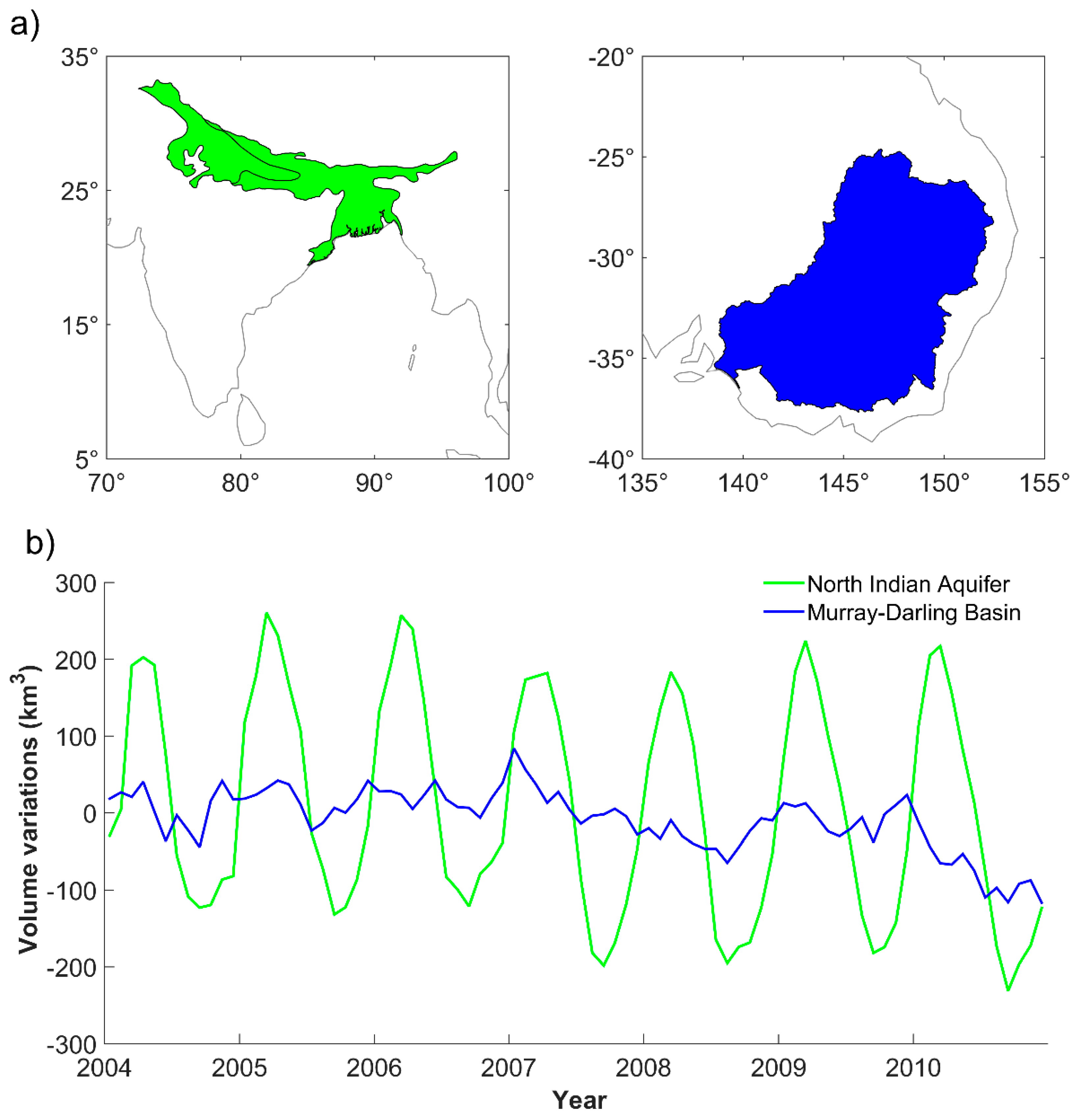
5.1. Groundwater Depletion

The new information on TWS anomaly provided, for the very first time at global scale, by the GRACE mission when combined with external information (see Section 3), allowed for the detection of changes in GWS in the major aquifer worldwide. In most of the major aquifers that were located in arid and semi-arid areas at mid-latitude, large depletion rates were identified, resulting from an excess of water extraction due to intensive pumping when compared with the natural recharge from infiltration. Examples of GWS time-series are presented in Figure 5. Large aquifer depletion rates, down to ~−60 mm·year−1 of GWS loss in EWH, were estimated in North Africa, Middle East, India, China, Australia, and the USA (Table 1). In many of these regions, high agricultural productivity is obtained through the use of GW for irrigation [12].
As it can be seen in Table 1, large variations can be observed over the same area from different studies. These apparent discrepancies can be accounted for several factors that include the accuracy of the GRACE datasets (processing center, release, global, or regional solutions), the completeness of the external information, the period on which the trends were estimated. The two former reasons will be analyzed in Section 6. Discussion. The latter one is perfectly illustrated in the case of the Sacramento and San Joaquin River Basins that encompass the Californian Central Valley aquifer. Using almost the same datasets, except for the snow, changes in GWS of −3.1 ± 0.6 and −6.9 ± 1.3 km3·year−1 were found over the periods October 2002–March 2010 and April 2006–March 2003, respectively [60,92]. They result from an acceleration of the depletion that started in the mid-2000’s due to the over abstraction that was caused by intensive irrigation practices [103] Similar accelerations in the decline of GWS were also observed in several locations that were related to persistent drought as in Iran [104].

5.2. Determining Groundwater Related Parameters Using GRACE-Based TWS

GRACE-derived TWS also provides useful information on groundwater related parameters. GW storage estimates obtained subtracting SM from the North America Land Data Assimilation System (NLDAS) to GRACE-based TWS, and well measurements were combined in a robust optimization approach, minimizing the negative impact of uncertainty on the different datasets through the incorporation of boundary conditions, that allows for the retrieval of Sy. This method was applied in the interconnected Edward Trinity Plateau and Pecos Valley aquifers (area of 115,000 km2), in Texas, USA, between August 2002 and December, providing consistent Sy values in the different hydrogeological regions [112]. GRACE-based TWS were also used for predicting GW level change based on the downscaling the GRACE data using artificial neural network models. Test performed for different wells that are located across the US demonstrate the potential of this approach to predict water levels at monthly and season time-scales even in the case of extreme climate events [113].
GRACE-based TWS were also used to characterize the impact of both climate variability and man-induced effects on GWS. GRACE-based GWS anomalies were used to define a GRACE GW Index (GGWI) to quantify the aquifer depletion. This index was defined as the normalized deviation in GWS (i.e., the GWS deviation, given by the difference between the monthly value and its climatology, minus its mean and divided by its standard deviation). Applied to the Central Valley aquifer, California, it shows a good capacity to properly identified GW-related droughts when classical indexes, such as Palmer Drought Index (PDSI) or Standardized Precipitation Index (SPI), detect them with an advance of several months [114]. As GW is a threatened resource, GRACE-based TWS were used to assess groundwater through the Renewable Groundwater Stress (RGS) defined as the ratio between groundwater use and groundwater availability. These two quantities were obtained from the trend in GWS anomalies from GRACE (computed as in [94]) and the natural groundwater recharge (estimated as the vertical flux between the aquifer and bottom soil layer of CLM 4.0). This approach was applied to the world’s 37 largest aquifers to classify them into stress regimes are defined as Overstressed, Variable Stress, Human-dominated Stress, and Unstressed depending on the RGS ratio [115]. Similarly, the Total Groundwater Stress (TGS) was defined as the ratio between the volume of water of the aquifer and the trend in GWS anomalies from GRACE. The former term is estimated as the product between the effective thickness of the aquifer, the porosity, and the surface of the aquifer. TGS was used to determine the number of years until the water volume stored in the aquifers is depleted from 25% to 90% of its total capacity [107].

6. Discussion

The GRACE mission provided estimates of TWS anomalies from March 2002 to June 2017 that were offering an unprecedented source of information to study the terrestrial branch of the hydrological cycle. This unique dataset was used to estimate GWS using the approaches presented in Section 3. However, these methods are suffering from limitations due to the errors on the GRACE data, the non-consideration of some hydrological compartments, fluxes, and abstractions.

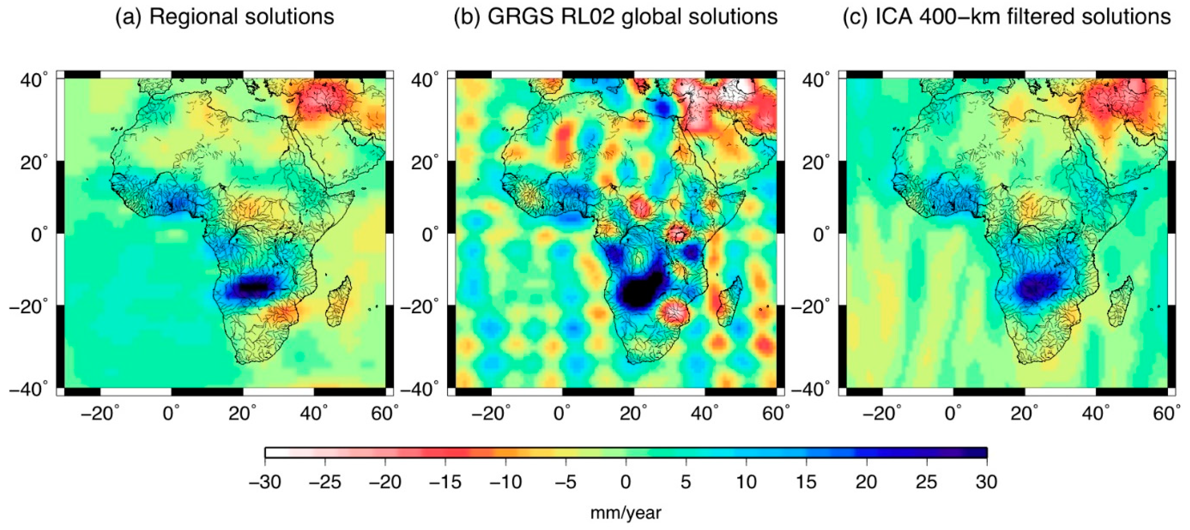
6.1. Sources of Errors in the GRACE Solutions

These are predominently of three types:
• Aliasing of short periods from correcting a priori models
Short time periods from hours to days of atmosphere and ocean tides are removed using dealiasing techniques based on corrections from models. While atmosphere pressure fields from ECMWF allow for a reasonable de-aliasing of high-frequency changes that are caused by non tidal atmospheric mass redistributions, errors due to tide model are present in the GRACE solutions, especially for diurnal (S1) and semi-diurnal (S2) tides [116,117,118,119]. Aliasing of the S2 tide has a strong impact on the determination on the degree-two order-zero harmonic coefficient of the geo-potential [120].
• North-South striping
The global Level-2 solutions describe the gravity signatures of un-modeled surface mass variations, mainly the seasonal water mass redistributions on ocean and land areas. Unfortunately, they are affected by north-south striping (see Figure 6), which is particularly visible in the tropical band where the coverage of the satellite tracks is poor because of (1) sparse GRACE track sampling in the longitudinal direction due to the polar orbit of the satellites, (2) propagation of systematic errors from the correcting model accelerations [116,117,118], and (3) strong numerical harmonic coefficient correlations that are generated by solving the undetermined systems of normal equations for high-degree Stokes coefficients [90].
• Spectral representation
Representation in spherical harmonics favors frequency description instead of spatial localization [122]. Stokes coefficients that were determined from GRACE measurements are provided as monthly (or 10-days) lists of harmonic coefficients of the geopotential, which were developed up to a fixed degree, such as 60 (equivalent spatial resolution of 333 km). Gibb’s effects create oscillations by omitting larger degree coefficients in the gravity signal reconstruction. This spectral truncation (or loss of energy) does not give access to the details of water mass fluxes at sub-continental scales (i.e., “leakage out”). Moreover, strong variations of hydrological signals in large drainage basins propagate on the entire sphere and pollute regional estimates in surrounding areas by unrealistic oscillations (i.e., “leakage in”) (e.g., see [100,123] for the cases of several large river basins).
To minimize the effects of the two latter sources of error, strategies to restore the GRACE signal in global solutions and local approaches were developed to be an alternative to the issues that are related to the classical global representation in spherical harmonics through the choice a suitable geometry of surface tiles. For the global solutions, the strategies can be directly based on water storage variations from hydrological model or LSM outputs (i.e., additive [124,125] and scaling factor [45] approaches) or indirectly (i.e., multiplicative approach [126], constrained [127] and unconstrained [72] forward modeling). Using a constrained forward modeling approach, the long term changes in GWS were reassessed in the northwest India aquifer [127]. A depletion rate of 31 ± 1 mm·year−1 (14.0 ± 0.4 km3·year−1) was found between January 2005 and December 2010, which is consistent with in situ measurements (28 mm·year−1 or 12.3 km3·year−1), but lower than the previously published ones (see Table 1), revealing a possible overestimate using classical techniques.
The local approaches are kown as Mascons (for mass concentrations) and regional approaches. In the Mascons approach, the variations of water mass are determined in rectangular elements, which are based on radar telemetry KBR, along the satellite tracks of GRACE, above the study area. The adjustment method of “regional” Stokes coefficients uses spatial and temporal constraints that induce a smoothing effect. Monthly Mascons solutions at 0.5° of spatial resolution were made available by CSR [128] and JPL [129]. Reduction of the leakage effect by 50% was obtained. The regional approach adjusts the surface densities of mass based on Level-1 GRACE data. This method is based on precise measurements on the K-band and the variations of speed between the two satellites. Contrary to the Mascons, the representation mode in spherical harmonics is not used. Therefore, the regional solutions are not affected by spectral truncation effects, and, besides, they provide a better geographical localization of hydrological patterns [130]. These solutions are not yet available globally but over continents, such as Africa [67], Australia [131], and South America [132]. Examples of TWS using regional and global approaches are presented in Figure 7.

6.2. Impacts of the Non Inclusion of Hydrological Water Compartments and Fluxes

The direct approach that is commonly used for estimating GWS anomalies assumes to take into account the water volume that is stored in the individual hydrological compartments. In many studies, LSM outputs were used to represent the other hydrological reservoirs than the GW. If the water that is contained in the other different hydrological reservoirs is occasionally accounted for, if available, using in situ data, abstractions for irrigation or the surface water stored in wetlands and on floodplains are generally not taken into account. In agricultural regions, taking into account the effect of irrigation on GWS changes from direct measurements of irrigation (IRR and SM+IRR) or through proportionality of the difference between potential evapotranspiration (PET) and evapotranspiration (ET) rates (Soil Moisture Deficit–SMD) strongly improves the quality of the estimates when compared to the classical approach. In three different regions of the High Plains Aquifer, r2 between in situ and GRACE-based estimates increased from 0.18 to 0.73 and 0.79 in the Northern High Plains Aquifer, 0 to 0.81 and 0.93 in the Central High Plains Aquifer and from 0.02 to 0.44 and 0.72 in the Southern High Plains Aquifer, USA, between 2003 and 2013, taking into account SMS, SMS+IRR, or SMD (both methods give the same results) and IRR [111]. In large river basins with extensive floodplains, SWS cannot be neglected, representing, for instance, between 40% and 50% of the annual variations of TWS as in the Amazon [133,134], Orinoco [135], and Ganges [136,137] basins. Regional SWS water changes can be estimated using multi-satellite observations, such as the synergy between inundation extent from satellite images and either satellite altimetry or Global Digital Elevation Models (GDEM). The first approach was used over the Negro River [70] and the Lower Ob’ [71] basins. It will be soon extended with the future launch of the NASA/CNES Surface Water and Ocean Topography (SWOT) that will provide global maps of water levels at 100 m of spatial resolution over land (in the water mask) [138].

7. Conclusions

During its sixteen years of operation, from March 2002 to June 2017, the GRACE mission provided a novel source of information on TWS variations at unprecedented spatial and temporal resolutions. It offered an exceptional dataset for studying large-scale water mass redistributions, and for the very first time, the opportunity to monitor groundwater changes from regional to global scales. GRACE data were widely used for characterizing the aquifers depletion in vast regions, large drainage areas, and transboundary aquifers, retrieving ground-water related parameters, such as the specific yield and developing new indices to identify aquifer depletion and GW stress. When the GRACE mission ended in 2017, a partnership between NASA and the German Research Centre for Geosciences (GFZ) decided to schedule the launch of the GRACE Follow-On (GRACE-FO) in 2018 in order to ensure continuity of GRACE-type space gravimetry. By using the same twin satellite configuration of low-Earth and the nearly polar orbit of 300–500 km, the GRACE-FO mission will be following its successful predecessor. Additionally, it will carry a demonstrator of laser system to measure the inter-satellite distance and velocity and for an improved precision. It is expected to provide new perspectives in hydrology studies, e.g., refined long-term mass balance estimates of surface water storage and ice sheets. Regional/local approaches have already demonstrated the possible access to spatial (better localization of structures by construction) and temporal (through daily updates using Kalman filter strategies [139,140]) scales that were lower than those that were offered by global solutions. These new data that will offer continuity with the previous GRACE measurements will be very useful for the purpose of global hydrology of global hydrological model calibration and to constrain their operations through assimilation techniques. In spite of its value, GRACE-FO data will still suffer the same limitations, as pointed out by [141]: (i) one-dimensional information for a three-dimensional aquifer; (ii) a coarse resolution incompatible with GW resources management, and (iii) inability to address issues that are related to GW pumping. The synergy with Interferometry Synthetic Aperture Radar (InSAR) data, which provides land subsidence, however, may give access to high resolution and quantitative GW changes maps that could be used to estimate aquifer reaction to pumping, to discriminate between climatic and anthopogenic storages changes and to assess aquifer confinement and dynamics [142]. A first demonstration of the synergy between the two techniques was performed in Central Mexico. Using ALOS-PALSAR images that were acquired between 2007 and 2011, areas subject to ground motion related to GW abstractions were detected. Due to the coarse resolution data, GW losses were only partly observed [142]. This encouraging first result offers new directions for GW studies.

Author Contributions

F.F. and G.R. conceived the study and wrote the paper.

Acknowledgments

We thank Pascal Gégout (GET-OMP) for fruitful discussions about the aliasing in the GRACE solutions. We are very thankful to Dr. Ehsan Forootan and three anonymous reviewers who helped us in improving the quality of our manuscript.

Conflicts of Interest

The authors declare no conflict of interest. The founding sponsors had no role in the design of the study; in the collection, analyses, or interpretation of data; in the writing of the manuscript, and in the decision to publish the results.

References

  1. Oki, T.; Kanae, S. Global hydrological cycles and world water resources. Science 2006, 313, 1068–1072. [Google Scholar] [CrossRef] [PubMed]
  2. Zektser, I.S.; Loaiciga, H.A. Groundwater fluxes in the global hydrologic cycle: Past, present and future. J. Hydrol. 1993, 144, 405–427. [Google Scholar] [CrossRef]
  3. Jackson, R.B.; Carpenter, S.R.; Dahm, C.N.; McKnight, D.M.; Naiman, R.J.; Postel, S.L.; Running, S.W. Water in a changing world. Ecol. Appl. 2001, 11, 1027–1045. [Google Scholar] [CrossRef]
  4. Sophocleous, M. Interactions between groundwater and surface water: The state of the science. Hydrogeol. J. 2002, 10, 52–67. [Google Scholar] [CrossRef]
  5. Griebler, C.; Avramov, M. Groundwater ecosystem services: A review. Freshw. Sci. 2015, 34, 355–367. [Google Scholar] [CrossRef]
  6. Giordano, M. Global Groundwater? Issues and Solutions. Annu. Rev. Environ. Resour. 2009, 34, 153–178. [Google Scholar] [CrossRef]
  7. Siebert, S.; Burke, J.; Faures, J.M.; Frenken, K.; Hoogeveen, J.; Döll, P.; Portmann, F.T. Groundwater use for irrigation—A global inventory. Hydrol. Earth Syst. Sci. 2010, 14, 1863–1880. [Google Scholar] [CrossRef] [Green Version]
  8. Konikow, L.F.; Kendy, E. Groundwater depletion: A global problem. Hydrogeol. J. 2005, 13, 317–320. [Google Scholar] [CrossRef]
  9. Gleeson, T.; Wada, Y.; Bierkens, M.F.P.; van Beek, L.P.H. Water balance of global aquifers revealed by groundwater footprint. Nature 2012, 488, 197–200. [Google Scholar] [CrossRef] [PubMed]
  10. Wada, Y.; van Beek, L.P.H.; Sperna Weiland, F.C.; Chao, B.F.; Wu, Y.-H.; Bierkens, M.F.P. Past and future contribution of global groundwater depletion to sea-level rise. Geophys. Res. Lett. 2012, 39. [Google Scholar] [CrossRef]
  11. Konikow, L.F. Contribution of global groundwater depletion since 1900 to sea-level rise. Geophys. Res. Lett. 2011, 38. [Google Scholar] [CrossRef]
  12. Famiglietti, J.S. The global groundwater crisis. Nat. Clim. Chang. 2014, 4, 945–948. [Google Scholar] [CrossRef]
  13. Konikow, L.F. Long-Term Groundwater Depletion in the United States. Groundwater 2015, 53, 2–9. [Google Scholar] [CrossRef] [PubMed]
  14. Zektser, I.S.; Everett, L.G. Groundwater Resources of the World: And Their Use; UNESCO: Paris, France, 2004; Volume 6, ISBN 9292200070. [Google Scholar]
  15. Shah, T. 10_Groundwater: A global assessment of scale and significance. In Water for Food, Water for Life: A Comprehensive Assessment of Water Management in Agriculture; Routledge: London, UK, 2007; pp. 395–423. [Google Scholar]
  16. Döll, P. Vulnerability to the impact of climate change on renewable groundwater resources: A global-scale assessment. Environ. Res. Lett. 2009, 4, 035006. [Google Scholar] [CrossRef]
  17. Gleeson, T.; VanderSteen, J.; Sophocleous, M.A.; Taniguchi, M.; Alley, W.M.; Allen, D.M.; Zhou, Y. Groundwater sustainability strategies. Nat. Geosci. 2010, 3, 378–379. [Google Scholar] [CrossRef]
  18. Green, T.R.; Taniguchi, M.; Kooi, H.; Gurdak, J.J.; Allen, D.M.; Hiscock, K.M.; Treidel, H.; Aureli, A. Beneath the surface of global change: Impacts of climate change on groundwater. J. Hydrol. 2011, 405, 532–560. [Google Scholar] [CrossRef]
  19. Taylor, R.G.; Scanlon, B.; Döll, P.; Rodell, M.; van Beek, R.; Wada, Y.; Longuevergne, L.; Leblanc, M.; Famiglietti, J.S.; Edmunds, M.; et al. Ground water and climate change. Nat. Clim. Chang. 2013, 3, 322–329. [Google Scholar] [CrossRef] [Green Version]
  20. Tapley, B.D.; Bettadpur, S.; Ries, J.C.; Thompson, P.F.; Watkins, M.M. GRACE measurements of mass variability in the Earth system. Science 2004, 305, 503–505. [Google Scholar] [CrossRef] [PubMed]
  21. Tapley, B.D.; Bettadpur, S.; Watkins, M.; Reigber, C. The gravity recovery and climate experiment: Mission overview and early results. Geophys. Res. Lett. 2004, 31. [Google Scholar] [CrossRef]
  22. Wouters, B.; Bonin, J.A.; Chambers, D.P.; Riva, R.E.M.; Sasgen, I.; Wahr, J. GRACE, time-varying gravity, Earth system dynamics and climate change. Rep. Prog. Phys. 2014, 77, 116801. [Google Scholar] [CrossRef] [PubMed]
  23. Frappart, F.; Ramillien, G.; Seoane, L. Monitoring water mass redistributions on land and polar ice sheets using the grace gravimetry from space mission. In Land Surface Remote Sensing in Continental Hydrology; Elsevier: Amsterdam, The Netherlands, 2016; pp. 255–279. ISBN 978-0-08-101181-2. [Google Scholar]
  24. Andersen, O.B.; Seneviratne, S.I.; Hinderer, J.; Viterbo, P. GRACE-derived terrestrial water storage depletion associated with the 2003 European heat wave. Geophys. Res. Lett. 2005, 32. [Google Scholar] [CrossRef]
  25. Chen, J.L.; Wilson, C.R.; Tapley, B.D.; Yang, Z.L.; Niu, G.Y. 2005 drought event in the Amazon River basin as measured by GRACE and estimated by climate models. J. Geophys. Res. 2009, 114. [Google Scholar] [CrossRef]
  26. Long, D.; Shen, Y.; Sun, A.; Hong, Y.; Longuevergne, L.; Yang, Y.; Li, B.; Chen, L. Drought and flood monitoring for a large karst plateau in Southwest China using extended GRACE data. Remote Sens. Environ. 2014, 155, 145–160. [Google Scholar] [CrossRef]
  27. Frappart, F.; Ramillien, G.; Famiglietti, J.S. Water balance of the Arctic drainage system using GRACE gravimetry products. Int. J. Remote Sens. 2011, 32, 431–453. [Google Scholar] [CrossRef] [Green Version]
  28. Syed, T.H.; Famiglietti, J.S.; Rodell, M.; Chen, J.; Wilson, C.R. Analysis of terrestrial water storage changes from GRACE and GLDAS. Water Resour. Res. 2008, 44. [Google Scholar] [CrossRef]
  29. Syed, T.H.; Famiglietti, J.S.; Chambers, D.P. GRACE-Based Estimates of Terrestrial Freshwater Discharge from Basin to Continental Scales. J. Hydrometeorol. 2009, 10, 22–40. [Google Scholar] [CrossRef]
  30. Rodell, M.; Famiglietti, J.S.; Chen, J.; Seneviratne, S.I.; Viterbo, P.; Holl, S.; Wilson, C.R. Basin scale estimates of evapotranspiration using GRACE and other observations. Geophys. Res. Lett. 2004, 31, L20504. [Google Scholar] [CrossRef]
  31. Ramillien, G.; Frappart, F.; Güntner, A.; Ngo-Duc, T.; Cazenave, A.; Laval, K. Time variations of the regional evapotranspiration rate from Gravity Recovery and Climate Experiment (GRACE) satellite gravimetry. Water Resour. Res. 2006, 42. [Google Scholar] [CrossRef] [Green Version]
  32. Rodell, M.; Famiglietti, J.S. The potential for satellite-based monitoring of groundwater storage changes using GRACE: The High Plains aquifer, Central US. J. Hydrol. 2002, 263, 245–256. [Google Scholar] [CrossRef]
  33. Schmidt, R.; Flechtner, F.; Meyer, U.; Neumayer, K.-H.; Dahle, C.; König, R.; Kusche, J. Hydrological Signals Observed by the GRACE Satellites. Surv. Geophys. 2008, 29, 319–334. [Google Scholar] [CrossRef]
  34. NASA JPL Space images. Available online: https://www.jpl.nasa.gov/spaceimages/images/largesize/PIA04235_hires.jpg (accessed on 10 November 2017).
  35. Wolff, M. Direct measurements of the Earth’s gravitational potential using a satellite pair. J. Geophys. Res. 1969, 74, 5295–5300. [Google Scholar] [CrossRef]
  36. Wahr, J.; Molenaar, M.; Bryan, F. Time variability of the Earth’s gravity field: Hydrological and oceanic effects and their possible detection using GRACE. J. Geophys. Res. Solid Earth 1998, 103, 30205–30229. [Google Scholar] [CrossRef]
  37. Integrated System Data Center. Available online: http://isdc.gfz-potsdam.de (accessed on 10 November 2017).
  38. Physical Oceanography Distributive Active Data Center. Available online: http://podaac.jpl.nasa.gov/GRACE (accessed on 10 November 2017).
  39. Tapley, B.D.; Reigber, C. The GRACE mission: Status and Early Results. In Proceedings of the Grace Science Team Meeting, Austin, TX, USA, 8–10 October 2003; pp. 41–63. [Google Scholar]
  40. Reigber, C.; Schmidt, R.; Flechtner, F.; König, R.; Meyer, U.; Neumayer, K.H.; Schwintzer, P.; Zhu, S.Y. An Earth gravity field model complete to degree and order 150 from GRACE: EIGEN-GRACE02S. J. Geodyn. 2005, 39, 1–10. [Google Scholar] [CrossRef]
  41. Tapley, B.; Ries, J.; Bettadpur, S.; Chambers, D.; Cheng, M.; Condi, F.; Gunter, B.; Kang, Z.; Nagel, P.; Pastor, R.; et al. GGM02—An improved Earth gravity field model from GRACE. J. Geod. 2005, 79, 467–478. [Google Scholar] [CrossRef]
  42. Ramillien, G.; Frappart, F.; Seoane, L. Space Gravimetry Using GRACE Satellite Mission: Basic Concepts. In Microwave Remote Sensing of Land Surfaces: Techniques and Methods; Elsevier: Amsterdam, The Netherlands, 2016; pp. 285–302. ISBN 978-0-08-101768-5. [Google Scholar]
  43. Rodell, M.; Famiglietti, J.S. Detectability of variations in continental water storage from satellite observations of the time dependent gravity field. Water Resour. Res. 1999, 35, 2705–2723. [Google Scholar] [CrossRef]
  44. Swenson, S.; Wahr, J.; Milly, P.C.D. Estimated accuracies of regional water storage variations inferred from the Gravity Recovery and Climate Experiment (GRACE). Water Resour. Res. 2003, 39. [Google Scholar] [CrossRef]
  45. Landerer, F.W.; Swenson, S.C. Accuracy of scaled GRACE terrestrial water storage estimates. Water Resour. Res. 2012, 48. [Google Scholar] [CrossRef]
  46. Geruo, A.; Wahr, J.; Zhong, S. Computations of the viscoelastic response of a 3-D compressible earth to surface loading: An application to glacial isostatic adjustment in Antarctica and Canada. Geophys. J. Int. 2013, 192, 557–572. [Google Scholar] [CrossRef]
  47. Sella, G.F.; Stein, S.; Dixon, T.H.; Craymer, M.; James, T.S.; Mazzotti, S.; Dokka, R.K. Observation of glacial isostatic adjustment in “stable” North America with GPS. Geophys. Res. Lett. 2007, 34, L02306. [Google Scholar] [CrossRef]
  48. Milne, G.A.; Davis, J.L.; Mitrovica, J.X.; Scherneck, H.G.; Johansson, J.M.; Vermeer, M.; Koivula, H. Space-geodetic constraints on glacial isostatic adjustment in Fennoscandia. Science 2001, 291, 2381–2385. [Google Scholar] [CrossRef] [PubMed]
  49. Yeh, P.J.-F.; Swenson, S.C.; Famiglietti, J.S.; Rodell, M. Remote sensing of groundwater storage changes in Illinois using the Gravity Recovery and Climate Experiment (GRACE). Water Resour. Res. 2006, 42. [Google Scholar] [CrossRef]
  50. Strassberg, G.; Scanlon, B.R.; Chambers, D. Evaluation of groundwater storage monitoring with the GRACE satellite: Case study of the High Plains aquifer, central United States. Water Resour. Res. 2009, 45. [Google Scholar] [CrossRef]
  51. Swenson, S.; Famiglietti, J.; Basara, J.; Wahr, J. Estimating profile soil moisture and groundwater variations using GRACE and Oklahoma Mesonet soil moisture data. Water Resour. Res. 2008, 44. [Google Scholar] [CrossRef]
  52. Rodell, M.; Houser, P.R.; Jambor, U.; Gottschalck, J.; Mitchell, K.; Meng, C.-J.; Arsenault, K.; Cosgrove, B.; Radakovich, J.; Bosilovich, M.; et al. The Global Land Data Assimilation System. Bull. Am. Meteorol. Soc. 2004, 85, 381–394. [Google Scholar] [CrossRef]
  53. Döll, P.; Kaspar, F.; Lehner, B. A global hydrological model for deriving water availability indicators: Model tuning and validation. J. Hydrol. 2003, 270, 105–134. [Google Scholar] [CrossRef]
  54. Van Dijk, A.I.J.M. The Australian Water Resources Assessment System, Technical report 3, Landscape Model (version 0.5) Technical Description; CSIRO: Canberra, ACT, Australia, 2010. [Google Scholar]
  55. Strassberg, G.; Scanlon, B.R.; Rodell, M. Comparison of seasonal terrestrial water storage variations from GRACE with groundwater-level measurements from the High Plains Aquifer (USA). Geophys. Res. Lett. 2007, 34, L14402. [Google Scholar] [CrossRef]
  56. Munier, S.; Becker, M.; Maisongrande, P.; Cazenave, A. Using grace to detect groundwater storage variations: the cases of canning basin and guarani aquifer system. Int. Water Technol. J. 2012, 2, 2–13. [Google Scholar]
  57. Khaki, M.; Forootan, E.; Kuhn, M.; Awange, J.; van Dijk, A.I.J.M.; Schumacher, M.; Sharifi, M.A. Determining water storage depletion within Iran by assimilating GRACE data into the W3RA hydrological model. Adv. Water Resour. 2018, 114, 1–18. [Google Scholar] [CrossRef]
  58. Leblanc, M.J.; Tregoning, P.; Ramillien, G.; Tweed, S.O.; Fakes, A. Basin-scale, integrated observations of the early 21st century multiyear drought in southeast Australia. Water Resour. Res. 2009, 45. [Google Scholar] [CrossRef]
  59. Shamsudduha, M.; Taylor, R.G.; Longuevergne, L. Monitoring groundwater storage changes in the highly seasonal humid tropics: Validation of GRACE measurements in the Bengal Basin. Water Resour. Res. 2012, 48. [Google Scholar] [CrossRef] [Green Version]
  60. Famiglietti, J.S.; Lo, M.; Ho, S.L.; Bethune, J.; Anderson, K.J.; Syed, T.H.; Swenson, S.C.; de Linage, C.R.; Rodell, M. Satellites measure recent rates of groundwater depletion in California’s Central Valley. Geophys. Res. Lett. 2011, 38. [Google Scholar] [CrossRef]
  61. Huang, J.; Halpenny, J.; van der Wal, W.; Klatt, C.; James, T.S.; Rivera, A. Detectability of groundwater storage change within the Great Lakes Water Basin using GRACE. J. Geophys. Res. Solid Earth 2012, 117. [Google Scholar] [CrossRef]
  62. Tiwari, V.M.; Wahr, J.; Swenson, S. Dwindling groundwater resources in northern India, from satellite gravity observations. Geophys. Res. Lett. 2009, 36, L18401. [Google Scholar] [CrossRef]
  63. Rodell, M.; Velicogna, I.; Famiglietti, J.S. Satellite-based estimates of groundwater depletion in India. Nature 2009, 460, 999–1002. [Google Scholar] [CrossRef] [PubMed]
  64. Werth, S.; White, D.; Bliss, D.W. GRACE Detected Rise of Groundwater in the Sahelian Niger River Basin. J. Geophys. Res. Solid Earth 2017. [Google Scholar] [CrossRef]
  65. Chen, J.L.; Wilson, C.R.; Tapley, B.D.; Scanlon, B.; Güntner, A. Long-term groundwater storage change in Victoria, Australia from satellite gravity and in situ observations. Glob. Planet. Chang. 2016, 139, 56–65. [Google Scholar] [CrossRef]
  66. Becker, M.; LLovel, W.; Cazenave, A.; Güntner, A.; Crétaux, J.-F. Recent hydrological behavior of the East African great lakes region inferred from GRACE, satellite altimetry and rainfall observations. Comptes Rendus Geosci. 2010, 342, 223–233. [Google Scholar] [CrossRef]
  67. Ramillien, G.; Frappart, F.; Seoane, L. Application of the regional water mass variations from GRACE satellite gravimetry to large-scale water management in Africa. Remote Sens. 2014, 6, 7379–7405. [Google Scholar] [CrossRef]
  68. Voss, K.A.; Famiglietti, J.S.; Lo, M.; de Linage, C.; Rodell, M.; Swenson, S.C. Groundwater depletion in the Middle East from GRACE with implications for transboundary water management in the Tigris-Euphrates-Western Iran region. Water Resour. Res. 2013, 49, 904–914. [Google Scholar] [CrossRef] [PubMed]
  69. Longuevergne, L.; Wilson, C.R.; Scanlon, B.R.; Crétaux, J.F. GRACE water storage estimates for the Middle East and other regions with significant reservoir and lake storage. Hydrol. Earth Syst. Sci. 2013, 17, 4817–4830. [Google Scholar] [CrossRef] [Green Version]
  70. Frappart, F.; Papa, F.; Güntner, A.; Werth, S.; Santos da Silva, J.; Tomasella, J.; Seyler, F.; Prigent, C.; Rossow, W.B.; Calmant, S.; et al. Satellite-based estimates of groundwater storage variations in large drainage basins with extensive floodplains. Remote Sens. Environ. 2011, 115, 1588–1594. [Google Scholar] [CrossRef] [Green Version]
  71. Frappart, F.; Papa, F.; Güntner, A.; Werth, S.; Ramillien, G.; Prigent, C.; Rossow, W.B.; Bonnet, M.-P. Interannual variations of the terrestrial water storage in the lower ob’ basin from a multisatellite approach. Hydrol. Earth Syst. Sci. 2010, 14, 2443–2453. [Google Scholar] [CrossRef] [Green Version]
  72. Ramillien, G.; Frappart, F.; Cazenave, A.; Güntner, A. Time variations of land water storage from an inversion of 2 years of GRACE geoids. Earth Planet. Sci. Lett. 2005, 235, 283–301. [Google Scholar] [CrossRef] [Green Version]
  73. Frappart, F.; Ramillien, G.; Biancamaria, S.; Mognard, N.M.; Cazenave, A. Evolution of high-latitude snow mass derived from the GRACE gravimetry mission (2002–2004). Geophys. Res. Lett. 2006, 33. [Google Scholar] [CrossRef] [Green Version]
  74. Sun, A.Y.; Green, R.; Swenson, S.; Rodell, M. Toward calibration of regional groundwater models using GRACE data. J. Hydrol. 2012, 422–423, 1–9. [Google Scholar] [CrossRef]
  75. Haddad, O.B.; Tabari, M.M.R.; Fallah-Mehdipour, E.; Mariño, M.A. Groundwater Model Calibration by Meta-Heuristic Algorithms. Water Resour. Manag. 2013, 27, 2515–2529. [Google Scholar] [CrossRef]
  76. Hu, L.; Jiao, J.J. Calibration of a large-scale groundwater flow model using GRACE data: A case study in the Qaidam Basin, China. Hydrogeol. J. 2015, 23, 1305–1317. [Google Scholar] [CrossRef]
  77. Werth, S.; Güntner, A. Calibration analysis for water storage variability of the global hydrological model WGHM. Hydrol. Earth Syst. Sci. 2010, 14, 59–78. [Google Scholar] [CrossRef]
  78. Eicker, A.; Schumacher, M.; Kusche, J.; Döll, P.; Schmied, H.M. Calibration/Data Assimilation Approach for Integrating GRACE Data into the WaterGAP Global Hydrology Model (WGHM) Using an Ensemble Kalman Filter: First Results. Surv. Geophys. 2014, 35, 1285–1309. [Google Scholar] [CrossRef]
  79. Bonan, G.B.; Oleson, K.W.; Vertenstein, M.; Levis, S.; Zeng, X.; Dai, Y.; Dickinson, R.E.; Yang, Z.L. The land surface climatology of the community land model coupled to the NCAR community climate model. J. Clim. 2002, 15, 3123–3149. [Google Scholar] [CrossRef]
  80. Yeh, P.J.F.; Eltahir, E.A.B. Representation of water table dynamics in a land surface scheme. Part I: Model development. J. Clim. 2005, 18, 1861–1880. [Google Scholar] [CrossRef]
  81. Lo, M.-H.; Famiglietti, J.S.; Yeh, P.J.-F.; Syed, T.H. Improving parameter estimation and water table depth simulation in a land surface model using GRACE water storage and estimated base flow data. Water Resour. Res. 2010, 46. [Google Scholar] [CrossRef]
  82. Koster, R.D.; Suarez, M.J.; Ducharne, A.; Stieglitz, M.; Kumar, P. A catchment-based approach to modeling land surface processes in a general circulation model: 1. Model structure. J. Geophys. Res. Atmos. 2000, 105, 24809–24822. [Google Scholar] [CrossRef]
  83. Zaitchik, B.F.; Rodell, M.; Reichle, R.H.; Zaitchik, B.F.; Rodell, M.; Reichle, R.H. Assimilation of GRACE Terrestrial Water Storage Data into a Land Surface Model: Results for the Mississippi River Basin. J. Hydrometeorol. 2008, 9, 535–548. [Google Scholar] [CrossRef]
  84. Li, B.; Rodell, M.; Zaitchik, B.F.; Reichle, R.H.; Koster, R.D.; van Dam, T.M. Assimilation of GRACE terrestrial water storage into a land surface model: Evaluation and potential value for drought monitoring in western and central Europe. J. Hydrol. 2012, 446–447, 103–115. [Google Scholar] [CrossRef]
  85. Schumacher, M.; Kusche, J.; Döll, P. A systematic impact assessment of GRACE error correlation on data assimilation in hydrological models. J. Geod. 2016, 90, 537–559. [Google Scholar] [CrossRef]
  86. Khaki, M.; Schumacher, M.; Forootan, E.; Kuhn, M.; Awange, J.L.; van Dijk, A.I.J.M. Accounting for spatial correlation errors in the assimilation of GRACE into hydrological models through localization. Adv. Water Resour. 2017, 108, 99–112. [Google Scholar] [CrossRef]
  87. Khaki, M.; Ait-El-Fquih, B.; Hoteit, I.; Forootan, E.; Awange, J.; Kuhn, M. A two-update ensemble Kalman filter for land hydrological data assimilation with an uncertain constraint. J. Hydrol. 2017, 555, 447–462. [Google Scholar] [CrossRef]
  88. Tian, S.; Tregoning, P.; Renzullo, L.J.; van Dijk, A.I.J.M.; Walker, J.P.; Pauwels, V.R.N.; Allgeyer, S. Improved water balance component estimates through joint assimilation of GRACE water storage and SMOS soil moisture retrievals. Water Resour. Res. 2017, 53, 1820–1840. [Google Scholar] [CrossRef]
  89. Khaki, M.; Forootan, E.; Kuhn, M.; Awange, J.; Papa, F.; Shum, C.K. A study of Bangladesh’s sub-surface water storages using satellite products and data assimilation scheme. Sci. Total Environ. 2018, 625, 963–977. [Google Scholar] [CrossRef] [PubMed]
  90. Swenson, S.; Wahr, J. Post-processing removal of correlated errors in GRACE data. Geophys. Res. Lett. 2006, 33, L08402. [Google Scholar] [CrossRef]
  91. GRACE Tellus. Available online: https://grace.jpl.nasa.gov/ (accessed on 26 February 2018).
  92. Scanlon, B.R.; Longuevergne, L.; Long, D. Ground referencing GRACE satellite estimates of groundwater storage changes in the California Central Valley, USA. Water Resour. Res. 2012, 48. [Google Scholar] [CrossRef] [Green Version]
  93. Feng, W.; Zhong, M.; Lemoine, J.-M.; Biancale, R.; Hsu, H.-T.; Xia, J. Evaluation of groundwater depletion in North China using the Gravity Recovery and Climate Experiment (GRACE) data and ground-based measurements. Water Resour. Res. 2013, 49, 2110–2118. [Google Scholar] [CrossRef]
  94. Castle, S.L.; Thomas, B.F.; Reager, J.T.; Rodell, M.; Swenson, S.C.; Famiglietti, J.S. Groundwater depletion during drought threatens future water security of the Colorado River Basin. Geophys. Res. Lett. 2014, 41, 5904–5911. [Google Scholar] [CrossRef] [PubMed]
  95. Swenson, S.; Yeh, P.J.-F.; Wahr, J.; Famiglietti, J. A comparison of terrestrial water storage variations from GRACE with in situ measurements from Illinois. Geophys. Res. Lett. 2006, 33, L16401. [Google Scholar] [CrossRef]
  96. Ek, M.B.; Mitchell, K.E.; Lin, Y.; Rogers, E.; Grunmann, P.; Koren, V.; Gayno, G.; Tarpley, J.D. Implementation of Noah land surface model advances in the National Centers for Environmental Prediction operational mesoscale Eta model. J. Geophys. Res. 2003, 108, 8851. [Google Scholar] [CrossRef]
  97. Chinnasamy, P.; Hubbart, J.A.; Agoramoorthy, G.; Chinnasamy, P.; Hubbart, J.A.; Agoramoorthy, G. Using Remote Sensing Data to Improve Groundwater Supply Estimations in Gujarat, India. Earth Interact. 2013, 17, 1–17. [Google Scholar] [CrossRef]
  98. Fan, Y.; van den Dool, H. Climate Prediction Center global monthly soil moisture data set at 0.5° resolution for 1948 to present. J. Geophys. Res. 2004, 109, D10102. [Google Scholar] [CrossRef]
  99. Huang, Z.; Pan, Y.; Gong, H.; Yeh, P.J.-F.; Li, X.; Zhou, D.; Zhao, W. Subregional-scale groundwater depletion detected by GRACE for both shallow and deep aquifers in North China Plain. Geophys. Res. Lett. 2015, 42, 1791–1799. [Google Scholar] [CrossRef]
  100. Frappart, F.; Ramillien, G.; Leblanc, M.; Tweed, S.O.; Bonnet, M.-P.; Maisongrande, P. An independent component analysis filtering approach for estimating continental hydrology in the GRACE gravity data. Remote Sens. Environ. 2011, 115, 187–204. [Google Scholar] [CrossRef] [Green Version]
  101. Frappart, F.; Papa, F.; Famiglietti, J.S.; Prigent, C.; Rossow, W.B.; Seyler, F. Interannual variations of river water storage from a multiple satellite approach: A case study for the Rio Negro River basin. J. Geophys. Res. Atmos. 2008, 113. [Google Scholar] [CrossRef] [Green Version]
  102. Milly, P.C.D.; Shmakin, A.B. Global Modeling of Land Water and Energy Balances. Part I: The Land Dynamics (LaD) Model. J. Hydrometeorol. 2002, 3, 283–299. [Google Scholar] [CrossRef]
  103. Scanlon, B.R.; Faunt, C.C.; Longuevergne, L.; Reedy, R.C.; Alley, W.M.; McGuire, V.L.; McMahon, P.B. Groundwater depletion and sustainability of irrigation in the US High Plains and Central Valley. Proc. Natl. Acad. Sci. USA 2012, 109, 9320–9325. [Google Scholar] [CrossRef] [PubMed] [Green Version]
  104. Forootan, E.; Rietbroek, R.; Kusche, J.; Sharifi, M.A.; Awange, J.L.; Schmidt, M.; Omondi, P.; Famiglietti, J. Separation of large scale water storage patterns over Iran using GRACE, altimetry and hydrological data. Remote Sens. Environ. 2014, 140, 580–595. [Google Scholar] [CrossRef]
  105. Gonçalvès, J.; Petersen, J.; Deschamps, P.; Hamelin, B.; Baba-Sy, O. Quantifying the modern recharge of the “fossil” Sahara aquifers. Geophys. Res. Lett. 2013, 40, 2673–2678. [Google Scholar] [CrossRef]
  106. Ahmed, M.; Sultan, M.; Wahr, J.; Yan, E. The use of GRACE data to monitor natural and anthropogenic induced variations in water availability across Africa. Earth-Science Rev. 2014, 136, 289–300. [Google Scholar] [CrossRef]
  107. Richey, A.S.; Thomas, B.F.; Lo, M.H.; Famiglietti, J.S.; Swenson, S.; Rodell, M. Uncertainty in global groundwater storage estimates in a Total Groundwater Stress framework. Water Resour. Res. 2015, 51, 5198–5216. [Google Scholar] [CrossRef] [PubMed]
  108. Joodaki, G.; Wahr, J.; Swenson, S. Estimating the human contribution to groundwater depletion in the Middle East, from GRACE data, land surface models, and well observations. Water Resour. Res. 2014, 50, 2679–2692. [Google Scholar] [CrossRef]
  109. Chen, J.; Li, J.; Zhang, Z.; Ni, S. Long-term groundwater variations in Northwest India from satellite gravity measurements. Glob. Planet. Chang. 2014, 116, 130–138. [Google Scholar] [CrossRef]
  110. Shen, H.; Leblanc, M.; Tweed, S.; Liu, W. Groundwater depletion in the Hai River Basin, China, from in situ and GRACE observations. Hydrol. Sci. J. 2015, 60, 671–687. [Google Scholar] [CrossRef]
  111. Breña-Naranjo, J.A.; Kendall, A.D.; Hyndman, D.W. Improved methods for satellite-based groundwater storage estimates: A decade of monitoring the high plains aquifer from space and ground observations. Geophys. Res. Lett. 2014, 41, 6167–6173. [Google Scholar] [CrossRef]
  112. Sun, A.Y.; Green, R.; Rodell, M.; Swenson, S. Inferring aquifer storage parameters using satellite and in situ measurements: Estimation under uncertainty. Geophys. Res. Lett. 2010, 37. [Google Scholar] [CrossRef]
  113. Sun, A.Y. Predicting groundwater level changes using GRACE data. Water Resour. Res. 2013, 49, 5900–5912. [Google Scholar] [CrossRef]
  114. Thomas, B.F.; Famiglietti, J.S.; Landerer, F.W.; Wiese, D.N.; Molotch, N.P.; Argus, D.F. GRACE Groundwater Drought Index: Evaluation of California Central Valley groundwater drought. Remote Sens. Environ. 2017, 198, 384–392. [Google Scholar] [CrossRef]
  115. Richey, A.S.; Thomas, B.F.; Lo, M.-H.; Reager, J.T.; Famiglietti, J.S.; Voss, K.; Swenson, S.; Rodell, M. Quantifying renewable groundwater stress with GRACE. Water Resour. Res. 2015, 51, 5217–5238. [Google Scholar] [CrossRef] [PubMed]
  116. Han, S.-C.; Jekeli, C.; Shum, C.K. Time-variable aliasing effects of ocean tides, atmosphere, and continental water mass on monthly mean GRACE gravity field. J. Geophys. Res. Solid Earth 2004, 109. [Google Scholar] [CrossRef]
  117. Thompson, P.F.; Bettadpur, S.V.; Tapley, B.D. Impact of short period, non-tidal, temporal mass variability on GRACE gravity estimates. Geophys. Res. Lett. 2004, 31. [Google Scholar] [CrossRef]
  118. Ray, R.D.; Luthcke, S.B. Tide model errors and GRACE gravimetry: Towards a more realistic assessment. Geophys. J. Int. 2006, 167, 1055–1059. [Google Scholar] [CrossRef]
  119. Forootan, E.; Didova, O.; Schumacher, M.; Kusche, J.; Elsaka, B. Comparisons of atmospheric mass variations derived from ECMWF reanalysis and operational fields, over 2003–2011. J. Geod. 2014, 88, 503–514. [Google Scholar] [CrossRef]
  120. Seo, K.W.; Wilson, C.R.; Chen, J.; Waliser, D.E. GRACE’s spatial aliasing error. Geophys. J. Int. 2008, 172, 41–48. [Google Scholar] [CrossRef]
  121. Frappart, F.; Ramillien, G.; Maisongrande, P.; Bonnet, M.-P. Denoising satellite gravity signals by independent component analysis. IEEE Geosci. Remote Sens. Lett. 2010, 7, 421–425. [Google Scholar] [CrossRef] [Green Version]
  122. Freeden, W.; Schreiner, M. Spherical Functions of Mathematical Geosciences; Springer: New York, NY, USA, 2009; ISBN 978-3-54-085112-7. [Google Scholar]
  123. Ramillien, G.; Lombard, A.; Cazenave, A.; Ivins, E.R.; Llubes, M.; Remy, F.; Biancale, R. Interannual variations of the mass balance of the Antarctica and Greenland ice sheets from GRACE. Glob. Planet. Chang. 2006, 53, 198–208. [Google Scholar] [CrossRef]
  124. Klees, R.; Zapreeva, E.A.; Winsemius, H.C.; Savenije, H.H.G. The bias in GRACE estimates of continental water storage variations. Hydrol. Earth Syst. Sci. 2007, 11, 1227–1241. [Google Scholar] [CrossRef]
  125. Longuevergne, L.; Scanlon, B.R.; Wilson, C.R. GRACE Hydrological estimates for small basins: Evaluating processing approaches on the High Plains Aquifer, USA. Water Resour. Res. 2010, 46. [Google Scholar] [CrossRef]
  126. Swenson, S.; Wahr, J. Multi-sensor analysis of water storage variations of the Caspian Sea. Geophys. Res. Lett. 2007, 34. [Google Scholar] [CrossRef]
  127. Long, D.; Chen, X.; Scanlon, B.R.; Wada, Y.; Hong, Y.; Singh, V.P.; Chen, Y.; Wang, C.; Han, Z.; Yang, W. Have GRACE satellites overestimated groundwater depletion in the Northwest India Aquifer? Sci. Rep. 2016, 6, 24398. [Google Scholar] [CrossRef] [PubMed] [Green Version]
  128. Save, H.; Bettadpur, S.; Tapley, B.D. High-resolution CSR GRACE RL05 mascons. J. Geophys. Res. Solid Earth 2016, 121, 7547–7569. [Google Scholar] [CrossRef]
  129. Wiese, D.N.; Landerer, F.W.; Watkins, M.M. Quantifying and reducing leakage errors in the JPL RL05M GRACE mascon solution. Water Resour. Res. 2016, 52, 7490–7502. [Google Scholar] [CrossRef]
  130. Ramillien, G.L.; Seoane, L.; Frappart, F.; Biancale, R.; Gratton, S.; Vasseur, X.; Bourgogne, S. Constrained Regional Recovery of Continental Water Mass Time-variations from GRACE-based Geopotential Anomalies over South America. Surv. Geophys. 2012, 33, 887–905. [Google Scholar] [CrossRef] [Green Version]
  131. Seoane, L.; Ramillien, G.; Frappart, F.; Leblanc, M. Regional GRACE-based estimates of water mass variations over Australia: Validation and interpretation. Hydrol. Earth Syst. Sci. 2013, 17, 4925–4939. [Google Scholar] [CrossRef]
  132. Frappart, F.; Seoane, L.; Ramillien, G. Validation of GRACE-derived terrestrial water storage from a regional approach over South America. Remote Sens. Environ. 2013, 137, 69–83. [Google Scholar] [CrossRef]
  133. Frappart, F.; Papa, F.; Santos Da Silva, J.; Ramillien, G.; Prigent, C.; Seyler, F.; Calmant, S. Surface freshwater storage and dynamics in the Amazon basin during the 2005 exceptional drought. Environ. Res. Lett. 2012, 7, 044010. [Google Scholar] [CrossRef] [Green Version]
  134. Papa, F.; Frappart, F.; Güntner, A.; Prigent, C.; Aires, F.; Getirana, A.C.V.; Maurer, R. Surface freshwater storage and variability in the Amazon basin from multi-satellite observations, 1993–2007. J. Geophys. Res. Atmos. 2013, 118, 11951–11965. [Google Scholar] [CrossRef]
  135. Frappart, F.; Papa, F.; Malbeteau, Y.; León, J.G.; Ramillien, G.; Prigent, C.; Seoane, L.; Seyler, F.; Calmant, S. Surface freshwater storage variations in the orinoco floodplains using multi-satellite observations. Remote Sens. 2015, 7, 89–110. [Google Scholar] [CrossRef]
  136. Papa, F.; Frappart, F.; Malbeteau, Y.; Shamsudduha, M.; Vuruputur, V.; Sekhar, M.; Ramillien, G.; Prigent, C.; Aires, F.; Pandey, R.K.; et al. Satellite-derived surface and sub-surface water storage in the Ganges-Brahmaputra River Basin. J. Hydrol. Reg. Stud. 2015, 4, 15–35. [Google Scholar] [CrossRef]
  137. Salameh, E.; Frappart, F.; Papa, F.; Güntner, A.; Venugopal, V.; Getirana, A.; Prigent, C.; Aires, F.; Labat, D.; Laignel, B. Fifteen years (1993–2007) of surface freshwater storage variability in the ganges-brahmaputra river basin using multi-satellite observations. Water 2017, 9, 245. [Google Scholar] [CrossRef]
  138. Biancamaria, S.; Lettenmaier, D.P.; Pavelsky, T.M. The SWOT Mission and Its Capabilities for Land Hydrology. Surv. Geophys. 2016, 37, 307–337. [Google Scholar] [CrossRef]
  139. Kurtenbach, E.; Eicker, A.; Mayer-Gürr, T.; Holschneider, M.; Hayn, M.; Fuhrmann, M.; Kusche, J. Improved daily GRACE gravity field solutions using a Kalman smoother. J. Geodyn. 2012, 59–60, 39–48. [Google Scholar] [CrossRef]
  140. Ramillien, G.L.; Frappart, F.; Gratton, S.; Vasseur, X. Sequential estimation of surface water mass changes from daily satellite gravimetry data. J. Geod. 2015, 89, 259–282. [Google Scholar] [CrossRef]
  141. Alley, W.M.; Konikow, L.F. Bringing GRACE Down to Earth. Groundwater 2015, 53, 826–829. [Google Scholar] [CrossRef] [PubMed]
  142. Castellazzi, P.; Martel, R.; Galloway, D.L.; Longuevergne, L.; Rivera, A. Assessing Groundwater Depletion and Dynamics Using GRACE and InSAR: Potential and Limitations. Groundwater 2016, 54, 768–780. [Google Scholar] [CrossRef] [PubMed]
Figure 1. Artist view of the Gravity Recovery and Climate Experiment (GRACE) mission. Source: [34].
Remotesensing 10 00829 g001
Figure 2. Variations against the latitude of the free air gravitational anomaly (red) (a) correlated with the surface topography along the satellites trajectory (blue) and with changes in the inter-satellite distance (black) as measured by the K-band ranging (KBR) system (b). Corresponding ground track overflying part of the Indian Ocean, India, the mountainous region of Himalaya, Siberia, and the Arctic Ocean (red) (c). Source: [39].
Remotesensing 10 00829 g002
Figure 3. Terrestrial trends estimated over 2004–2010 from (a) Gravity Recovery and Climate Experiment (GRACE)-based Terrestrial Water Storage (TWS) anomalies (GFZ RL05 GRACE solutions preprocessed using the destriping technique from [90] and smoothed at 300 km of radius) corrected from GIA from [46], (b) soil moisture (SM) and snow from Global Land Data Assimilation System (GLDAS)-NOAH 2.7.1 [52] and (c) difference between TWS from GRACE corrected from GIA and SM and snow for the whole land surfaces. These datasets were made available by [91].
Remotesensing 10 00829 g003
Figure 4. Time variations of the groundwater (GW) storage from GRACE and external information (black) in different locations of the Negro-River basin (Amazon): (a) in the Asu catchment (in situ GW storage in gray), (b,c) in the swamps of Caapiranga and Morro da Água Preta, respectively (altimetry-derived SW storage in gray), from [70].
Remotesensing 10 00829 g004
Figure 5. GW declines affect a lot of regions in the world such as the North Indian Aquifer (green) and the Murray-Darling Basin (blue) (a). Time variations of monthly GW storage from January 2004 to December 2010 over the North Indian Aquifer (green) and the Murray-Darling Basin exhibit the depletion of several tenths of km3. GWS were estimated as the difference between TWS from GRACE (GFZ RL05 solutions) and SM (and snow) from GLDAS NOAH 2.7.1 (b).
Remotesensing 10 00829 g005
Figure 6. Synthetic GRACE-based anomaly of mass for March 2006 obtained combining ocean bottom pressure from the Estimating the Circulation and Climate of the Ocean (ECCO) model, TWS from WaterGAP Global Hydrology Model (WGHM) and north-south stripes obtained as the differences between level-1 and level-2 GRACE solutions (top). The application of a filter (here using the Independent Component Analysis) allows for the separation of the land and ocean signals (middle) from the north–south stripes (bottom). Source: [121].
Remotesensing 10 00829 g006
Figure 7. Comparison of maps of water mass linear trends computed using different GRACE-related products: (a) regional 2° × 2° mascon-like solutions; (b) Centre National d’Etudes Spatiales/Groupe de Recherche en Géodésie Spatiale (CNES/GRGS) Spherical Harmonics (SH) solutions revealing important unrealistic North-South striping and (c) linear combination of SH solutions through Independent Component Analysis (ICA). Source: [67].
Remotesensing 10 00829 g007
Table 1. Annual rates of groundwater depletion in the major aquifers located in arid and semi-arid regions based on the decomposition of GRACE-based TWS.
RegionArea 106 km2CountriesEstimated Depletion RateGRACE Product and ReleaseSM ProductSW ProductSnow ProductPeriod (MM/YYYY–MM/YYYY)Ref
mm·year−1km3·year−1
Northwestern Sahara Aquifer System1Algeria, Lybia, Tunisia−0.54  ±  1.40−0.54  ±  1.40NAGLDASNoneNone01/2003–12/2007[105]
−0.81 ± 0.16−0.81 ± 0.16CSR 05NoneNoneNone01/2003–09/2012[106]
−4.48−4.48RegionalNoneNoneNone06/2003–12/2012[67]
2.69  ±  0.8−2.69  ±  0.8CSR 05GLDASCLM 0.4None01/2003–12/2013[107]
Nubian Sandstone Aquifer System2.2Chad, Egypt, Lybia, Sudan−3.72 ± 0.27−8.18 ± 0.59CSR 05NoneNoneNone01/2003–09/2012[106]
−2.76 ± 0.86−6.08  ±  1.9CSR 05GLDASCLM 0.4None01/2003–12/2013[107]
Tigris and Euphrates River Basin0.75Turkey, Syria, Iraq, Iran−27.2 ± 0.6−20.4 ± 0.45CSR 05GLDASAltimetryNone01/2003–12/2009[68]
Middle EastNAIrak, Iran, Saudi Arabia, TurkeyNA−43 ± 3CSR 05CLM 4.5CLM 4.5 + AltimetryNone02/2003–12/2012[108]
Northwest India0.56India−40 ± 10−17.7 ± 4.5CSR 04GLDASNoneGLDAS08/2002–10/2008[63]
−47.7 ± 12−20.4 ± 7.1CSR 05GLDASNoneGLDAS01/2003–12/2012 [109]
Norhern India2.7India−20 ± 3−54 ± 9CSR 04CLMCLMGLDAS04/2002–06/2008[62]
North China0.37China−22 ± 3−8.3 ± 1.1CSR 05GLDASNoneNone01/2003–12/2010[93]
Hai River China−17.0 ± 4.3−5.5 ± 1.4GRGS 2In situIn situNone01/2003–12/2012[110]
−8.3 ± 4.5−2.7 ± 5.5CSR 05
Piedmont Plain0.054China−46.5 ± 6.8−2.5 ± 0.4CSR 05GLDASNoneNone01/2003–07/2013[99]
East Central Plain0.086China−16.9 ± 1.9−1.5 ± 0.2CSR 05GLDASNoneNone01/2003–07/2013[99]
Canning0.43Australia−25.6−11GRGS 2NOAHNoneNone01/2003–12/2009[56]
Murray Darling Basin1Australia−17 ± 717 ± 7GRGS 1NOAHIn situNone01/2003–12/2007[58]
−17.2 ± 4.717.2 ± 4.7CSR 05WGHMWGHMNone01/2003–12/2012[65]
High Plains Aquifer0.45USA−25.1 ± 2.1−11.4 ± 0.4CSR 05NOAHIn situNone03/2003–02/2013[111]
Sacramento and San Joaquin River Basins0.154USA−20.4 ± 3.9−3.1 ± 0.6CSR 04GLDASIn situNORHSC10/2002–03/2010[60]
−55.9 ± 5.3−8.6 ± 0.8GRGS 2GLDASIn situSNODAS04/2006–03/2010[92]
−44.9 ± 8.5−6.9 ± 1.3CSR 04GLDASIn situSNODAS04/2006–03/2010[92]
Colorado River Basin0.64USA8.75 ± 0.63−5.6 ± 0.4CSR 05GLDASIn situSNODAS12/2004–11/2013[94]

