Diurnal Variation of Light Absorption in the Yellow River Estuary


Abstract
1. Introduction
2. Data and Methods
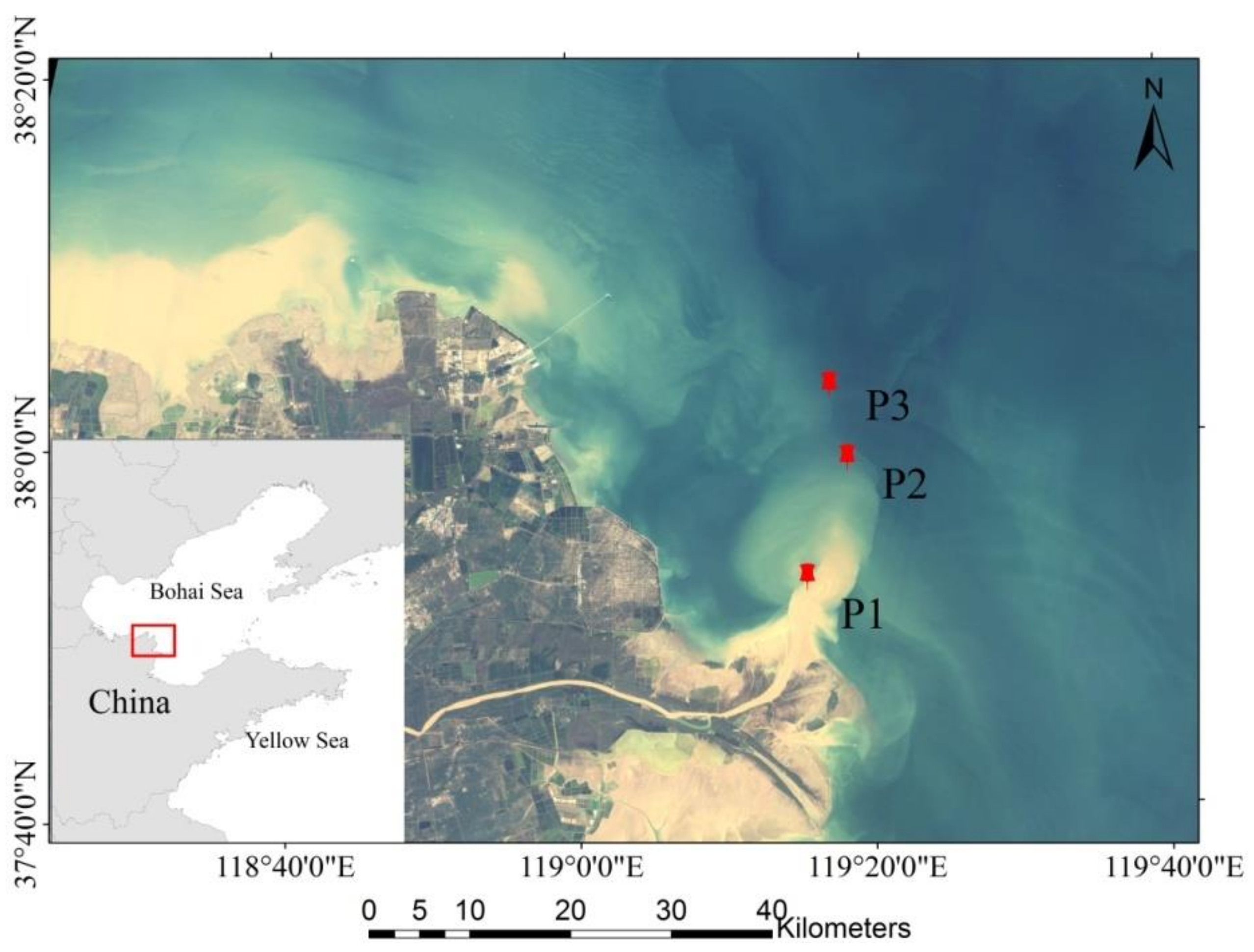
2.1. Study Area
2.2. Data Collection
2.2.1. Measurement of Suspended Particle Matter Concentration
2.2.2. Measurement of Chlorophyll-a Concentration
2.2.3. Measurement of Light Absorption of Seawater
2.2.4. Remote Sensing Reflectance
2.3. Data Analysis
3. Results
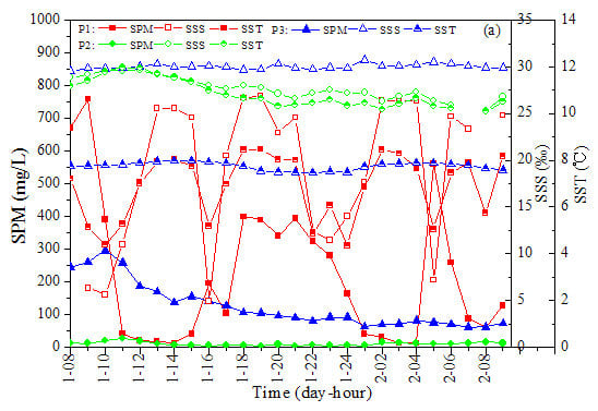
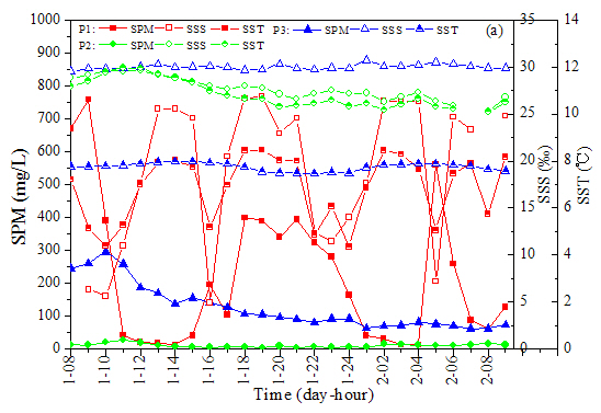
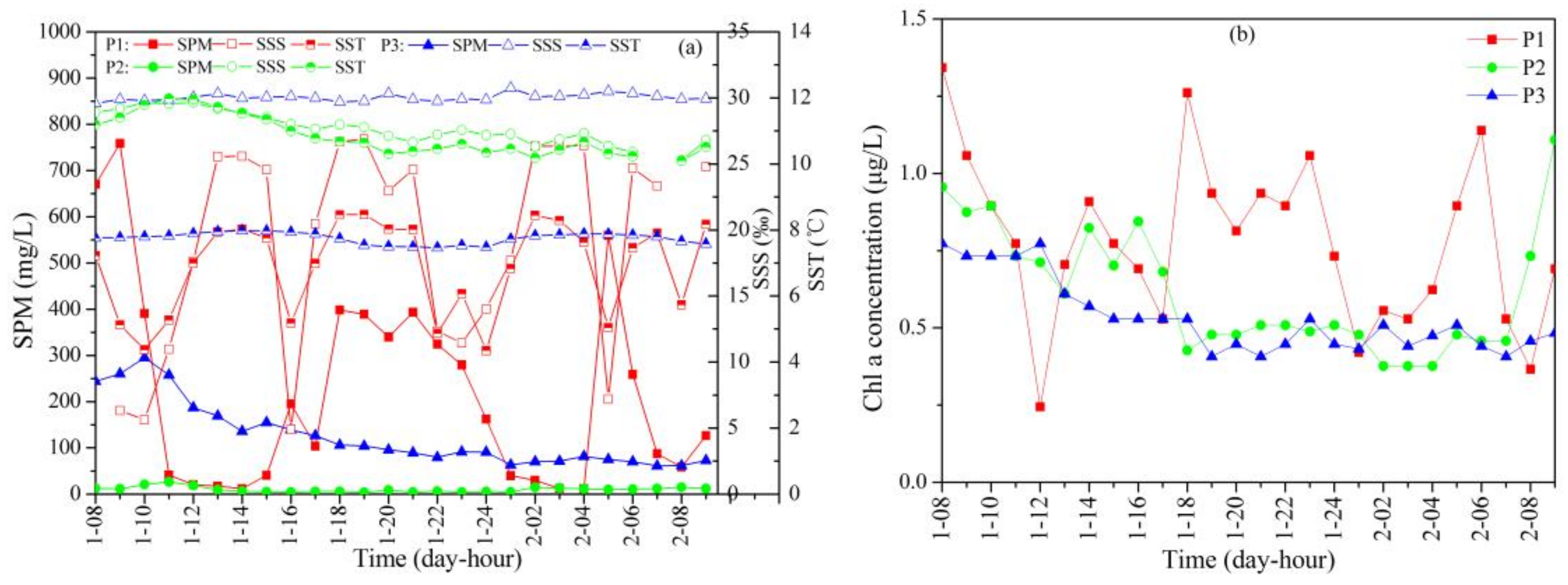
3.1. SPM and Chl-a Concentrations
3.2. CDOM Absorption
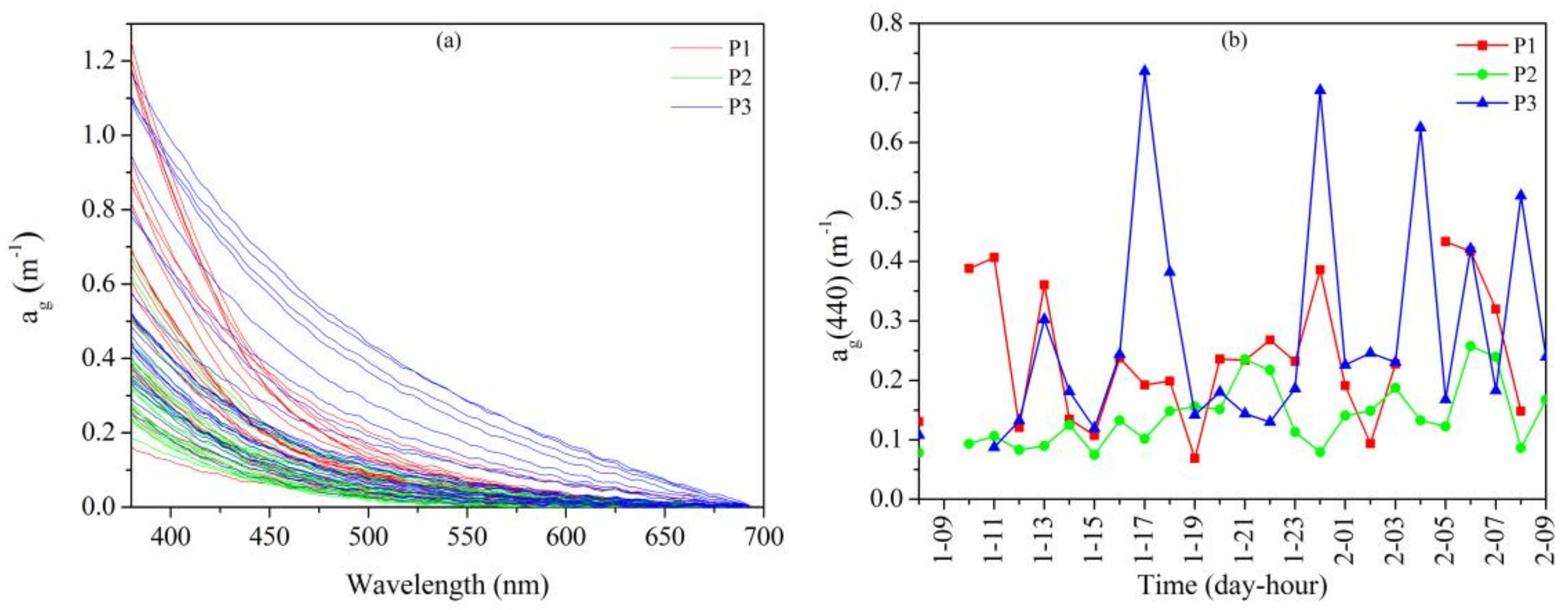
3.2.1. Diurnal Variation of CDOM Absorption
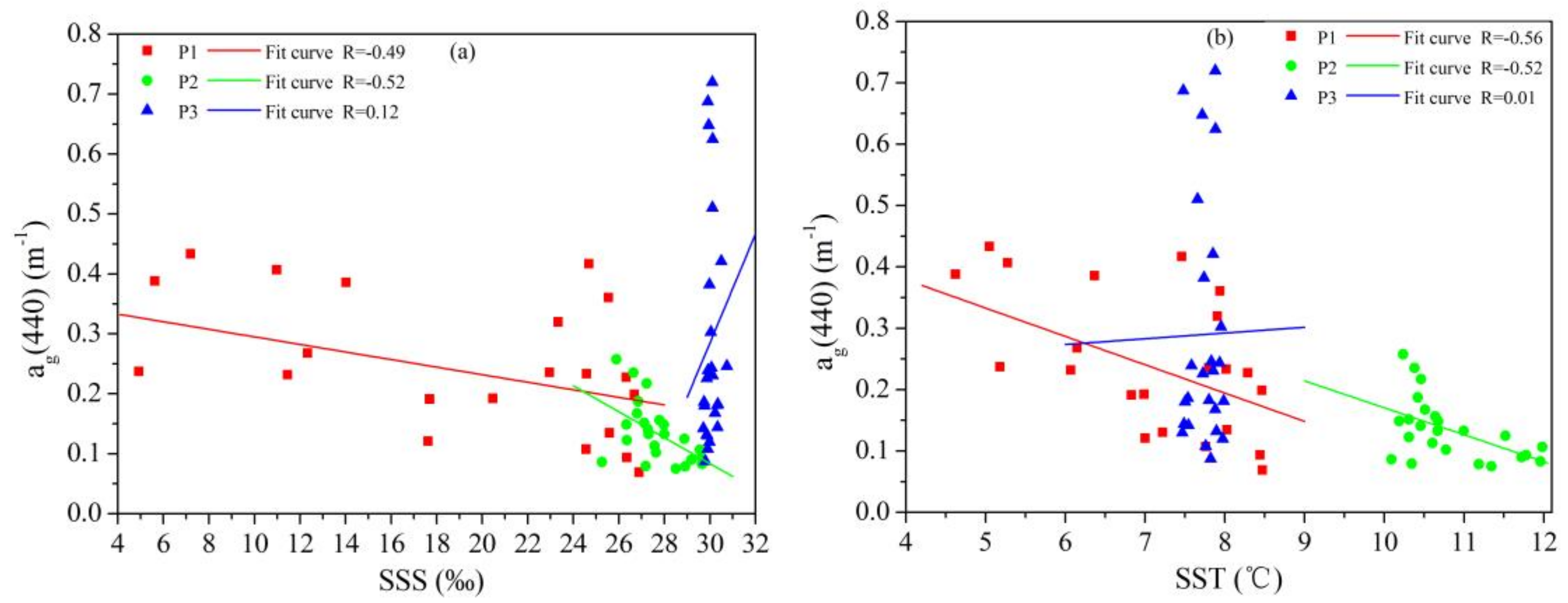
3.2.2. Relationship between CDOM Absorption and Salinity or Temperature
3.2.3. Spectral Slope of CDOM Absorption
3.3. Particles Absorption
3.3.1. Total Particle Absorption
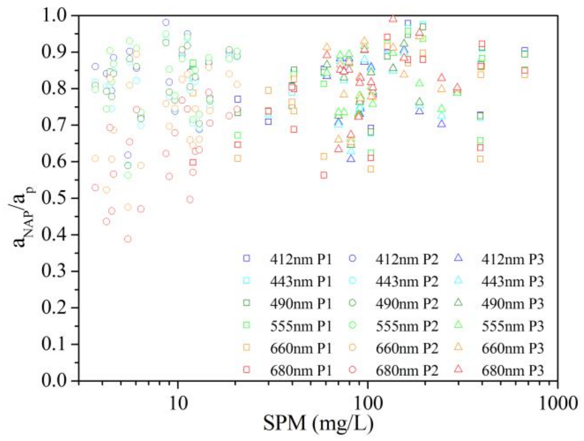
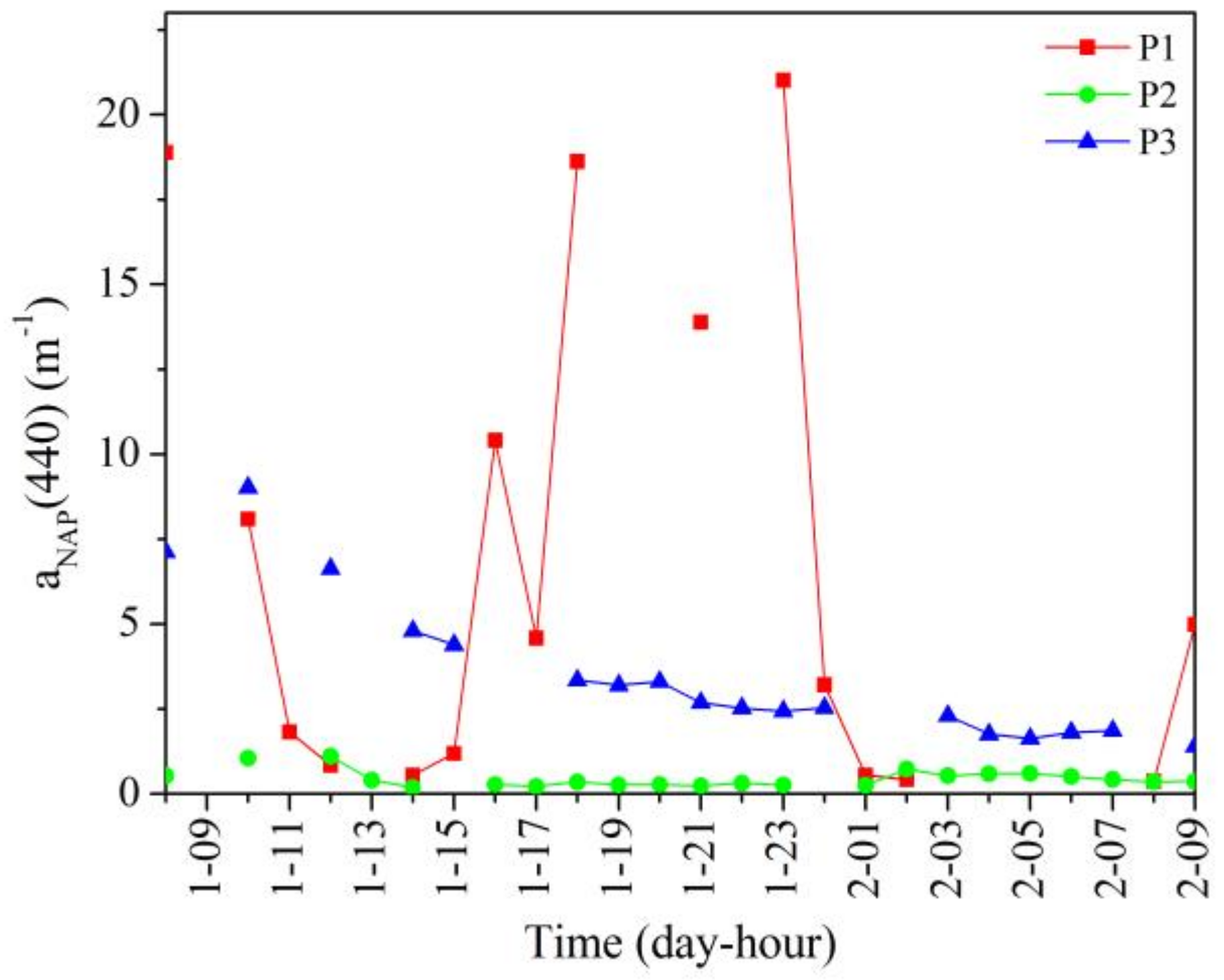
3.3.2. Non-Algal Particle Absorption
3.4. Total Water Absorption
3.5. Diurnal Variation of Remote Sensing Reflectance
4. Discussion
4.1. Diurnal Variation of Light Absorption
4.1.1. CDOM Absorption
4.1.2. Particles Absorption
4.1.3. Total Water Absorption
4.2. Factors Affecting Light Absorption Diurnal Variation
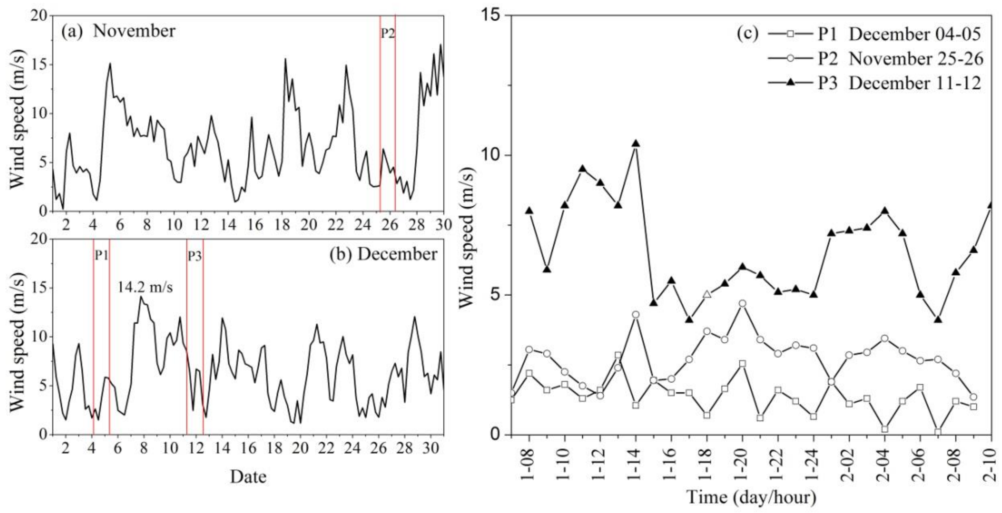
4.2.1. Strong Winds
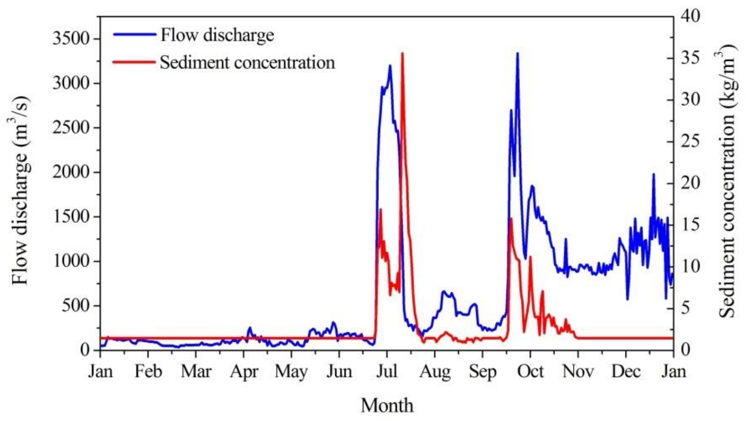
4.2.2. Yellow River Discharge
4.2.3. Tidal Cycle
4.3. Implications of Diurnal Variation for Remote Sensing Products
5. Conclusions
Acknowledgments
Author Contributions
Conflicts of Interest
References
- Vecchio, R.D.; Blough, N.V. Influence of ultraviolet radiation on the chromophoric dissolved organic matter in natural waters. In Environmental UV Radiation: Impact on Ecosystems and Human Health and Predictive Models, Proceedings of the NATO Advanced Study Institute, Pisa, Italy, 30 April–10 May 2001; Ghetti, F., Checcucci, G., Bornman, J.F., Eds.; NATO Science Series: IV; Earth and Environmental Sciences; Springer: Berlin, Germany, 2006; Volume 57. [Google Scholar]
- Hargreaves, B.R. Water column optics and penetration of UVR. In UV Effects in Aquatic Organisms and Ecosystems; Helbling, E.W., Zagarese, H., Eds.; The Royal Society of Chemistry: Cambridge, UK, 2003; Volume 1, pp. 59–108. [Google Scholar]
- Antoine, D.; André, J.M.; Morel, A. Oceanic primary production: II. Estimation at global scale from satellite (Coastal Zone Color Scanner) chlorophyll. Glob. Biogeochem. Cycles 1996, 10, 57–69. [Google Scholar] [CrossRef]
- Behrenfeld, M.J.; Falkowski, P.G. Photosynthetic rates derived from satellite based chlorophyll concentrations. Limnol. Oceanogr. 1997, 42, 1–20. [Google Scholar] [CrossRef]
- Xie, H.; Aubry, C.; Bélanger, S.; Song, G. The dynamics of absorption coefficients of CDOM and particles in the St. Lawrence estuarine system: Biogeochemical and physical implications. Mar. Chem. 2012, 128, 44–56. [Google Scholar] [CrossRef]
- Cui, T.W.; Cao, W.X.; Zhang, J.; Hao, Y.; Yu, Y.; Zu, T.T.; Wang, D.X. Diurnal variability of ocean optical properties during a coastal algal bloom: Implications for ocean colour remote sensing. Int. J. Remote Sens. 2013, 34, 8301–8318. [Google Scholar] [CrossRef]
- Woźniak, S.B.; Meler, J.; Lednicka, B.; Zdun, A.; Stoń-Egiert, J. Inherent optical properties of suspended particulate matter in the southern Baltic Sea. Oceanologia 2011, 53, 691–729. [Google Scholar]
- Mercado, J.M.; Ramírez, T.; Cortés, D.; Sebastián, M. Diurnal changes in the bio-optical properties of the phytoplankton in the Alborán Sea (Mediterranean Sea). Estuar. Coast. Shelf Sci. 2006, 69, 459–470. [Google Scholar] [CrossRef]
- Ohi, N.; Saito, H.; Taguchi, S. Diel patterns in chlorophyll a specific absorption coefficient and absorption efficiency factor of picoplankton. J. Oceanogr. 2005, 61, 379–388. [Google Scholar] [CrossRef]
- Bowers, D.; Evans, D.; Thomas, D.; Ellis, K.; Williams, P.J.L.B. Interpreting the colour of an estuary. Estuar. Coast. Shelf Sci. 2004, 59, 13–20. [Google Scholar] [CrossRef]
- Morel, A.; Prieur, L. Analysis of variations in ocean color. Limnol. Oceanogr. 1977, 22, 709–722. [Google Scholar] [CrossRef]
- D’Sa, E.J.; Ko, D.S. Short-term influences on suspended particulate matter distribution in the northern Gulf of Mexico: Satellite and model observations. Sensors 2008, 8, 4249–4264. [Google Scholar] [CrossRef] [PubMed]
- D’Sa, E.J.; Miller, R.L.; Del Castillo, C. Bio-optical properties and ocean color algorithms for coastal waters influenced by the Mississippi River during a cold front. Appl. Opt. 2006, 45, 7410–7428. [Google Scholar] [CrossRef] [PubMed]
- Siegel, D.A.; Maritorena, S.; Nelson, N.B.; Hansell, D.A.; Lorenzi-Kayser, M. Global distribution and dynamics of colored dissolved and detrital organic materials. J. Geophys. Res. Ocean. 2002, 107. [Google Scholar] [CrossRef]
- Zhou, H.L.; Zhu, J.H.; Li, T.J. Spectral properties of colored dissolved organic matter in Chinese offshore waters. J. Trop. Oceanogr. 2015, 34, 23–29, (In Chinese with English Abstract). [Google Scholar]
- Ruddick, K.; Vanhellemont, Q.; Yan, J.; Neukermans, G.; Wei, G. Variability of suspended particulate matter in the Bohai Sea from the geostationary Ocean Color Imager (GOCI). Ocean Sci. J. 2012, 47, 331–345. [Google Scholar] [CrossRef]
- Cui, T.; Zhang, J.; Groom, S.; Sun, L.; Smyth, T.; Sathyendranath, S. Validation of MERIS ocean-color products in the Bohai Sea: A case study for turbid coastal waters. Remote Sens. Environ. 2010, 114, 2326–2336. [Google Scholar] [CrossRef]
- Wei, H.; Sun, J.; Moll, A.; Zhao, L. Phytoplankton dynamics in the Bohai Sea-observations and modelling. J. Mar. Syst. 2004, 44, 233–251. [Google Scholar] [CrossRef]
- Wang, Q.; Guo, X.; Takeoka, H. Seasonal variations of the Yellow River plume in the Bohai Sea: A model study. J. Geophys. Res. 2008, 113, C08046. [Google Scholar] [CrossRef]
- Hu, F.; Gu, G. Seasonal changes of the mean tidal range along the Chinese coasts. Oceanol. Limnol. Sin. 1989, 20, 401–411. [Google Scholar]
- Hainbucher, D.; Hao, W.; Pohlmann, T.; Feng, S.; Suendermann, J. Variability of the Bohai Sea circulation based on model calculations. J. Mar. Syst. 2004, 44, 153–174. [Google Scholar] [CrossRef]
- Zhao, W.; Sun, L.; Cui, T.; Cao, W.; Ma, Y.; Hao, Y. Mapping the distribution of suspended particulate matter concentrations influenced by storm surge in the Yellow River Estuary using FY-3A MERSI 250-m data. Aquat. Ecosyst. Health 2014, 17, 290–298. [Google Scholar] [CrossRef]
- Zhang, M.; Tang, J.; Dong, Q.; Song, Q.; Ding, J. Retrieval of total suspended matter concentration in the Yellow and East China Seas from MODIS imagery. Remote Sens. Environ. 2010, 114, 392–403. [Google Scholar] [CrossRef]
- Choi, J.K.; Park, Y.J.; Ahn, J.H.; Lim, H.S.; Eom, J.; Ryu, J.H. GOCI, the world’s first geostationary ocean color observation satellite, for the monitoring of temporal variability in coastal water turbidity. J. Geophys. Res. 2012, 117, C09004. [Google Scholar] [CrossRef]
- Min, J.E.; Ryu, J.H.; Lee, S.; Son, S. Monitoring of suspended sediment variation using Landsat and MODIS in the Saemangeum coastal area of Korea. Mar. Pollut. Bull. 2012, 64, 382–390. [Google Scholar] [CrossRef] [PubMed]
- Van der Linde, D.W. Protocol for Determination of Total Suspended Matter in Oceans and Coastal Zones; Technical Note I.98.182; Joint Research Centre: Brussels, Belgium, 1998. [Google Scholar]
- Wang, G.; Cao, W.; Yang, Y.; Zhou, W.; Liu, S.; Yang, D. Variations in light absorption properties during a phytoplankton bloom in the Pearl River estuary. Cont. Shelf Res. 2010, 30, 1085–1094. [Google Scholar] [CrossRef]
- Parsons, T.R.; Maita, Y.; Lalli, C.M. A Manual of Chemical and Biological Methods for Seawater Analysis; Pergamon Press: Oxford, UK, 1984. [Google Scholar]
- Nima, C.; Frette, Ø.; Hamre, B.; Erga, S.R.; Chen, Y. Absorption properties of high-latitude Norwegian coastal water: The impact of CDOM and particulate matter. Estuar. Coast. Shelf Sci. 2016, 178, 158–167. [Google Scholar] [CrossRef]
- Mitchell, B.G.; Kahru, M.; Wieland, J.; Stramska, S. Determination of spectral absorption coefficients of particles, dissolved material and phytoplankton for discrete water samples. In Ocean Optics Protocols for Satellite Ocean Colour Sensor Validation; Mueller, J.L., Fargoin, G.S., McClain, C.R., Eds.; Revision 4, NASA/TM-2003-211621/Rev4-vol.4; NASA Goddard Space Flight Center: Greenbelt, MD, USA, 2003; Volume IV (Chapter 4), pp. 39–64. [Google Scholar]
- Tilstone, G.H.; Moore, G.F.; Sørensen, K.; Doerfeer, R.; Røttgers, R.; Ruddick, K.D.; Pasterkamp, R.; Jørgensen, P.V. Regional Validation of MERIS Chlorophyll Products in North Sea Coastal Waters; REVAMP Methodologies EVGI-CT-2001-00049; VRIJE Universiteit Amsterdam: Amsterdam, The Netherlands, 2001. [Google Scholar]
- Tassan, S.; Ferrari, G.M.; Bricaud, A.; Babin, M. Variability of the amplification factor of light absorption by filter-retained aquatic particles in the coastal environment. J. Plankton Res. 2000, 22, 659–668. [Google Scholar] [CrossRef][Green Version]
- Bricaud, A.; Morel, A.; Prieur, L. Absorption by dissolved organic matter of the sea (yellow substance) in the UV and visible domains. Limnol. Oceanogr. 1981, 26, 43–53. [Google Scholar] [CrossRef]
- Stedmon, C.A.; Markager, S.; Kaas, H. Optical properties and signatures of chrompophoric dissolved organic matter (CDOM) in Danish waters. Estuar. Coast. Shelf Sci. 2000, 51, 267–278. [Google Scholar] [CrossRef]
- Blough, N.V.; Del Vecchio, R. Chromophoric DOM in the coastal environment. In Biogeochemistry of Marine Dissolved Organic Matter; Hansell, D.A., Carlson, C.A., Eds.; Academic Press: San Diego, CA, USA, 2002; pp. 509–578. [Google Scholar]
- Twardowski, M.S.; Boss, E.; Sullivan, J.M.; Donaghay, P.L. Modeling the spectral shape of absorption by chromophoric dissolved organic matter. Mar. Chem. 2004, 89, 69–88. [Google Scholar] [CrossRef]
- Granskog, M.A.; Macdonald, R.W.; Mundy, C.-J.; Barber, D.G. Distribution, characteristics and potential impacts of chromophoric dissolved organic matter (CDOM) in Hudson Strait and Hudson Bay, Canada. Cont. Shelf Res. 2007, 27, 2032–2050. [Google Scholar] [CrossRef]
- Babin, M.; Stramski, D.; Ferrari, G.M.; Claustre, H.; Bricaud, A.; Obolenski, G.; Hoepffner, N. Variations in the light absorption coefficients of phytoplankton, nonalgal particles, and dissolved organic matter in coastal waters around Europe. J. Geophys. Res. 2003, 108. [Google Scholar] [CrossRef]
- Joshi, I.; D’Sa, E.J. Seasonal Variation of Colored Dissolved Organic Matter in Barataria Bay, Louisiana, Using Combined Landsat and Field Data. Remote Sens. 2015, 7, 12478–12502. [Google Scholar] [CrossRef]
- Zhang, X.Y.; Chen, X.; Deng, H.; Du, Y.; Jin, H.Y. Absorption features of chromophoric dissolved organic matter (CDOM) and tracing implication for dissolved organic carbon (DOC) in Changjiang Estuary, China. Biogeosci. Discuss. 2013, 10, 12217–12250. [Google Scholar] [CrossRef]
- Matsuoka, A.; Bricaud, A.; Benner, R.; Para, J.; Sempéré, R. Tracing the transport of colored dissolved organic matter in water masses of the Southern Beaufort Sea: Relationship with hydrographic characteristics. Biogeosci. Discusss. 2012, 9, 925–940. [Google Scholar] [CrossRef]
- Hong, H.; Wu, J.; Shang, S.; Hu, C. Absorption and fluorescence of chromophoric dissolved organic matter in the Pearl River Estuary, South China. Mar. Chem. 2005, 97, 78–89. [Google Scholar] [CrossRef]
- Kowalczuk, P.; Stoń-Egiert, J.; Cooper, W.J.; Whitehead, R.F.; Durako, M.J. Characterization of chromophoric dissolved organic matter (CDOM) in the Baltic Sea by excitation emission matrix fluorescence spectroscopy. Mar. Chem. 2005, 96, 273–292. [Google Scholar] [CrossRef]
- Cleveland, J.S. Regional models for phytoplankton absorption as a function of chlorophyll a concentration. J. Geophys. Res. 1995, 100, 13333–13344. [Google Scholar] [CrossRef]
- Bricaud, A.; Morel, A.; Babin, M.; Allali, K.; Claustre, H. Variations of light absorption by suspended particles with chlorophyll a concentration in oceanic (case 1) waters: Analysis and implications for bio-optical models. J. Geophys. Res. 1998, 103, 31033–31044. [Google Scholar] [CrossRef]
- Bricaud, A.; Babin, M.; Claustre, H.; Ras, J.; Tièche, F. Light absorption properties and absorption budget of Southeast Pacific waters. J. Geophys. Res. 2010, 115, C08009. [Google Scholar] [CrossRef]
- Shen, F.; Zhou, Y.; Hong, G. Absorption property of non-algal particles and contribution to total light absorption in optically complex waters, a case study in Yangtze Estuary and adjacent coast. Adv. Comput. Environ. Sci. 2012, 142, 61–66. [Google Scholar]
- Prieur, L.; Sathyendranath, S. An optical classification of coastal and oceanic waters based on the specific spectral absorption curves of phytoplankton pigments, dissolved organic matter, and other particulate materials. Limnol. Oceanogr. 1981, 26, 671–689. [Google Scholar] [CrossRef]
- Roesler, C.S.; Perry, M.J.; Carder, K.L. Modeling in situ phytoplankton absorption from total absorption spectra in productive inland marine waters. Limnol. Oceanogr. 1989, 34, 1510–1523. [Google Scholar] [CrossRef]
- Carder, K.L.; Hawes, S.K.; Baker, K.A.; Smith, R.C.; Steward, R.G.; Mitchell, B.G. Reflectance model for quantifying chlorohyll a in the presence of productivity degradation products. J. Geophys. Res. 1991, 96, 20599–20611. [Google Scholar] [CrossRef]
- Kirk, J.T.O. Light and Photosynthesis in Aquatic Ecosystems, 2nd ed.; Cambridge University Press: Cambridge, MD, USA, 1994. [Google Scholar]
- Monahan, E.C.; Pybus, M.J. Colour, ultraviolet absorbance and salinity of the surface waters off the west coast of Ireland. Nature 1978, 274, 782–784. [Google Scholar] [CrossRef]
- McKee, D.; Cunningham, A.; Jones, K. Simultaneous measurements of fluorescence and beam attenuation: Instrument characterisation and interpretation of signals from strati-fied coastal waters. Estuar. Coast. Shelf Sci. 1999, 48, 51–58. [Google Scholar] [CrossRef]
- Bowers, D.G.; Harker, G.E.L.; Smith, P.S.D.; Tett, P. Optical properties of a region of freshwater influence (the Clyde Sea). Estuar. Coast. Shelf Sci. 1999, 50, 717–726. [Google Scholar] [CrossRef]
- Bélanger, S.; Xie, H.; Krotkov, N.; Larouche, P.L.; Vincent, W.F.; Babin, M. Photomineralization of terrigenous dissolved organic matter in Arctic coastal waters from 1979 to 2003, Interannual variability and implications of climate change. Glob. Biogeochem. Cycles 2006, 20, GB4005. [Google Scholar] [CrossRef]
- Ferreira, A.; Ciotti, Á.M.; Coló Giannini, M.F. Variability in the light absorption coefficients of phytoplankton, nonalgal particles, and colored dissolved organic matter in a subtropical bay (Brazil). Estuar. Coast. Shelf Sci. 2014, 139, 127–136. [Google Scholar] [CrossRef]
- Bowers, D.G.; Brett, H.L. The relationship between CDOM and salinity in estuaries: An analytical and graphical solution. J. Mar. Syst. 2008, 73, 1–7. [Google Scholar] [CrossRef]
- Sasaki, H.; Siswanto, E.; Nishiuchi, K.; Tanaka, K.; Hasegawa, T.; Ishizaka, J. Mapping the low salinity Changjiang diluted water using satellite-retrieved colored dissolved organic matter (CDOM) in the East China Sea during high river flow season. Geophys. Res. Lett. 2008, 35, L04604. [Google Scholar] [CrossRef]
- Nieke, B.; Reuter, R.; Heuermann, R.; Wang, H.; Babin, M.; Therriault, J. Light absorption and fluorescence properties of chromophoric dissolved organic matter (CDOM) in the St. Lawrence estuary (Case 2 waters). Cont. Shelf Res. 1997, 17, 235–252. [Google Scholar] [CrossRef]
- Carder, K.L.; Steward, R.G.; Harvey, G.R.; Ortner, P.B. Marine humic and fulvic acids: Their effects on remote sensing of ocean chlorophyll. Limnol. Oceanogr. 1989, 34, 68–81. [Google Scholar] [CrossRef]
- Del Castillo, C.E.; Coble, P.G. Seasonal variability of the colored dissolved organic matter during the 1994–95 NE and SW monsoons in the Arabian Sea. Deep-Sea Res. 2000, 47, 1563–1579. [Google Scholar] [CrossRef]
- Schwarz, J.N.; Kowalczuk, P.; Kaczmarek, S. Two models for absorption by colored dissolved organic matter (CDOM). Oceanologia 2002, 44, 209–241. [Google Scholar]
- Duan, H.; Ma, R.H.; Kong, W.; Hao, J.Y.; Zhang, S. Optical properties of chromophoric dissolved organic matter in Lake Taihu. J. Lake Sci. 2009, 21, 242–247, (In Chinese with English Abstract). [Google Scholar]
- Xing, X.G.; Zhao, D.Z.; Liu, Y.G.; Yang, J.H.; Wang, L. Absorption characteristics of de-pigmented particle and yellow substance in Bohai Sea. Mar. Environ. Sci. 2008, 27, 595–598, (In Chinese with English Abstract). [Google Scholar]
- Bowers, D.G.; Harker, G.E.L.; Stephan, B. Absorption spectra of inorganic particles in the Irish Sea and their relevance to remote sensing of chlorophyll. Int. J. Remote Sens. 1996, 17, 2449–2460. [Google Scholar] [CrossRef]
- Bricaud, A.; Claustre, H.; Ras, J.; Oubelkheir, K. Natural variability of phytoplanktonic absorption in oceanic waters: Influence of the size structure of algal populations. J. Geophys. Res. 2004, 109, C11010. [Google Scholar] [CrossRef]
- Bricaud, A.; Babin, M.; Morel, A.; Claustre, H. Variability in the chlorophyllspecific absorption coefficients of natural phytoplankton: Analysis and parameterization. J. Geophys. Res. 1995, 100, 13321–13332. [Google Scholar] [CrossRef]
- Cao, P.; Huo, F.; Gu, G. Relationship between suspended sediments from the Changjiang estuary and the evolution of the embayed muddy coast of Zhejiang Province. Acta Oceanol. Sin. 1989, 8, 273–283. [Google Scholar]
- Su, J.L. Overview of the South China Sea circulation and its influence on the coastal physical oceanography outside the Pearl River Estuary. Cont. Shelf Res. 2004, 24, 1745–1760. [Google Scholar]
- Mao, Q.W.; Shi, P.; Yin, K.D.; Gan, J.P.; Qi, Y.Q. Tides and tidal currents in the Pearl River Estuary. Cont. Shelf Res. 2004, 24, 1797–1808. [Google Scholar] [CrossRef]
- Harrison, P.J.; Yin, K.D.; Gan, J.P.; Liu, H.B. Physical–biological coupling in the Pearl River Estuary. Cont. Shelf Res. 2008, 28, 1405–1415. [Google Scholar] [CrossRef]
- Cheng, Z.; Wang, X.H.; Paull, D.; Gao, J. Application of the Geostationary Ocean Color Imager to Mapping the Diurnal and Seasonal Variability of Surface Suspended Matter in a Macro-Tidal Estuary. Remote Sens. 2016, 8, 244. [Google Scholar] [CrossRef]
- Wang, H.; Wang, A.; Bi, N.; Zeng, X.; Xiao, H. Seasonal distribution of suspended sediment in the Bohai Sea, China. Cont. Shelf Res. 2014, 90, 17–32. [Google Scholar] [CrossRef]
- He, X.Q.; Bai, Y.; Pan, D.L.; Huang, N.L.; Dong, X.; Chen, J.S.; Chen, C.-T.A.; Cui, Q.F. Using geostationary satellite ocean color data to map the diurnal dynamics of suspended particulate matter in coastal waters. Remote Sens. Environ. 2013, 133, 225–239. [Google Scholar] [CrossRef]
- Yang, Z.; Liu, J. A unique Yellow River-derived distal subaqueous delta in the Yellow Sea. Mar. Geol. 2007, 240, 169–176. [Google Scholar] [CrossRef]
- Wang, H.; Saito, Y.; Zhang, Y.; Bi, N.; Sun, X.; Yang, Z. Recent changes of sediment flux to the western Pacific Ocean from major rivers in East and Southeast Asia. Earth-Sci. Rev. 2011, 108, 80–100. [Google Scholar] [CrossRef]
- Hu, B.; Li, G.; Li, J.; Bi, J.; Zhao, J.; Bu, R. Provenance and climate change inferred from Sr–Nd–Pb isotopes of late Quaternary sediments in the Huanghe (Yellow River) Delta, China. Quat. Res. 2012, 78, 561–571. [Google Scholar] [CrossRef]
- Hu, B.; Yang, Z.; Zhao, M.; Saito, Y.; Fan, D.; Wang, L. Grain size records reveal variability of the East Asian Winter Monsoon since the Middle Holocene in the Central Yellow Sea mud area, China. Sci. China Earth Sci. 2012, 55, 1656–1668. [Google Scholar] [CrossRef]
- Zang, Q.Y. Nearshore Sediment along the Yellow River Delta; Ocean Press: Beijing, China, 1996. (In Chinese) [Google Scholar]
- Qin, Y.S.; Li, F. Study on the suspended matter of the sea water of the Bohai gulf. Acta Oceanol. Sin. 1982, 4, 191–200. (In Chinese) [Google Scholar]
- Zhang, J.; Huang, W.W.; Liu, M.G. Distribution of suspended materials and its seasonal change in Huanghe River estuary as well as the nearby sea area. J. Shandong Coll. Oceanol. 1985, 15, 96–104. (In Chinese) [Google Scholar]
- Zhang, J.; Huang, W.W.; Shi, M.C. Huanghe (Yellow River) and its estuary: Sediment origin, transport and deposition. J. Hydrol. 1990, 120, 203–223. [Google Scholar] [CrossRef]
- Jiang, W.; Pohlmann, T.; Sündermann, J.; Feng, S. A modelling study of SPM transport in the Bohai Sea. J. Mar. Syst. 2000, 24, 175–200. [Google Scholar] [CrossRef]
- Wang, H.J.; Yang, Z.S.; Li, G.X.; Jiang, W.S. Wave climate modeling on the abandoned Huanghe (Yellow River) delta lobe and related deltaic erosion. J. Coast. Res. 2006, 22, 906–918. [Google Scholar] [CrossRef]
- Qiao, S.; Shi, X.; Zhu, A.; Liu, Y.; Bi, N.; Fang, X. Distribution and transport of suspended sediments off the Yellow River (Huanghe) mouth and the nearby Bohai Sea. Estuar. Coast. Shelf Sci. 2010, 86, 337–344. [Google Scholar] [CrossRef]
- Yang, Z.; Ji, Y.; Bi, N.; Lei, K.; Wang, H. Sediment transport of the Huanghe (Yellow River) delta and in the adjacent Bohai Sea in winter and seasonal comparison. Estuar. Coast. Shelf Sci. 2011, 93, 173–181. [Google Scholar] [CrossRef]
- Yang, Z.S.; Li, G.G.; Wang, H.J.; Hu, B.Q. Variation of daily water and sediment discharge in the lower reaches of Huanghe (Yellow River) in the past 55 years and its response to the dam operation on the mainstream. Mar. Geol. Quat. Geol. 2008, 28, 9–18. (In Chinese) [Google Scholar]
- Yang, S.; Ding, P.; Zhu, J.; Zhao, Q.; Mao, Z. Tidal flat morphodynamic processes of the Yangtze Estuary and their engineering implications. China Ocean Eng. 2000, 14, 307–320. [Google Scholar]
- Shi, W.; Wang, M.; Jiang, L. Spring-neap tidal effects on satellite ocean color observations in the Bohai Sea, Yellow Sea, and East China Sea. J. Geophys. Res. 2011, 116, C12032. [Google Scholar] [CrossRef]
- Shibata, T.; Tripathy, S.C.; Ishizaka, J. Phytoplankton pigment change as a photoadaptive response to light variation caused by tidal cycle in Ariake Bay, Japan. J. Oceanogr. 2010, 66, 831–843. [Google Scholar] [CrossRef]
- Uncles, R.J.; Barton, M.L.; Stephens, J.A. Seasonal variability of fine-sediment concentrations in the turbidity maximum region of the Tamar. Estuary. Estuar. Coast. Shelf Sci. 1994, 38, 19–39. [Google Scholar] [CrossRef]
- Uncles, R.J.; Stephens, J.A.; Smith, R.E. The dependence of estuarine turbidity on tidal intrusion length, tidal range and residence time. Cont. Shelf Res. 2002, 22, 1835–1856. [Google Scholar] [CrossRef]
- Bi, N.; Yang, Z.; Wang, H.; Hu, B.; Ji, Y. Sediment dispersion pattern off the present Huanghe (Yellow River) subdelta and its dynamic mechanism during normal river discharge period. Estuar. Coast. Shelf Sci. 2010, 86, 352–362. [Google Scholar] [CrossRef]
- Dall’Olmo, G.; Gitelson, A.A. Effect of Bio-Optical Parameter Variability and Uncertainties in Reflectance Measurements on the Remote Estimation of Chlorophyll-a Concentration in Turbid Productive Waters: Modeling Results. Appl. Opt. 2006, 45, 3577–3592. [Google Scholar] [CrossRef] [PubMed]
- Loisel, H.; Lubac, B.; Dessailly, D.; Duforet-Gaurier, L.; Vantrepotte, V. Effect of Inherent Optical Properties Variability on the Chlorophyll Retrieval from Ocean Colour Remote Sensing: An in Situ Approach. Opt. Express 2010, 18, 20949–20959. [Google Scholar] [CrossRef] [PubMed]
- Bailey, W.S.; Werdell, J.P. A Multi-Sensor Approach for the On-Orbit Validation of Ocean Colour Satellite Data Products. Remote Sens. Environ. 2006, 102, 12–23. [Google Scholar] [CrossRef]
- Mélin, F.; Zibordi, G.; Berthon, J.F. Assessment of Satellite Ocean Colour Products at a Coastal Site. Remote Sens. Environ. 2007, 110, 192–215. [Google Scholar] [CrossRef]
- Cui, T.; Zhang, J.; Tang, J.W.; Ma, Y.; Qing, S. Satellite Retrieval of Inherent Optical Properties in the Turbid Waters of the Yellow Sea and East China Sea. Chin. Opt. Lett. 2010, 8, 721–725. [Google Scholar]


| Stations | SPM (mg/L) | Chl-a (μg/L) | ||||||||
|---|---|---|---|---|---|---|---|---|---|---|
| Max. | Min. | Mean | SD | N | Max. | Min. | Mean | SD | N | |
| P1 | 758.69 | 11.92 | 220.00 | 216.44 | 26 | 1.34 | 0.24 | 0.78 | 0.27 | 26 |
| P2 | 26.45 | 3.67 | 9.95 | 5.68 | 26 | 1.11 | 0.38 | 0.62 | 0.20 | 26 |
| P3 | 295.22 | 60.87 | 125.09 | 69.67 | 26 | 0.77 | 0.41 | 0.53 | 0.12 | 26 |
| ag(440) | Max. (m−1) | Min. (m−1) | Mean (m−1) | SD (m−1) | N |
|---|---|---|---|---|---|
| P1 | 0.43 | 0.07 | 0.24 | 0.11 | 23 |
| P2 | 0.26 | 0.08 | 0.14 | 0.05 | 25 |
| P3 | 0.72 | 0.09 | 0.29 | 0.20 | 24 |
| Sg | Max. (nm−1) | Min. (nm−1) | Mean (nm−1) | SD (nm−1) | N |
|---|---|---|---|---|---|
| P1 | 0.021 | 0.012 | 0.017 | 0.002 | 23 |
| P2 | 0.020 | 0.012 | 0.016 | 0.002 | 25 |
| P3 | 0.018 | 0.008 | 0.013 | 0.003 | 24 |
| aNAP(440) | Max. (m−1) | Min. (m−1) | Mean (m−1) | SD (m−1) | N |
|---|---|---|---|---|---|
| P1 | 21.01 | 0.37 | 6.84 | 7.42 | 16 |
| P2 | 1.10 | 0.18 | 0.44 | 0.25 | 22 |
| P3 | 9.02 | 1.40 | 3.48 | 2.08 | 18 |
| Derived SNAP | Max | Min | Mean | SD | N |
|---|---|---|---|---|---|
| P1 | 0.0120 | 0.0104 | 0.0113 | 0.00042 | 16 |
| P2 | 0.0115 | 0.0100 | 0.0108 | 0.00035 | 22 |
| P3 | 0.0108 | 0.0097 | 0.0103 | 0.00029 | 18 |
| Rrs(680) (sr−1) | 22 September 2011 | 16 October 2011 | ||||||||
|---|---|---|---|---|---|---|---|---|---|---|
| Max. | Min. | Mean | SD | N | Max. | Min. | Mean | SD | N | |
| P1 | 0.0366 | 0.0140 | 0.0236 | 0.0092 | 8 | 0.0404 | 0.0137 | 0.02340 | 0.0091 | 8 |
| P2 | 0.0105 | 0.0053 | 0.0079 | 0.0019 | 8 | 0.0060 | 0.0041 | 0.0054 | 0.0007 | 8 |
| P3 | 0.0093 | 0.0035 | 0.0052 | 0.0017 | 8 | 0.0048 | 0.0031 | 0.0039 | 0.0006 | 8 |
| 25 October 2011 | 13 November 2011 | |||||||||
| P1 | 0.0421 | 0.0203 | 0.0280 | 0.0080 | 7 | 0.0383 | 0.0251 | 0.0341 | 0.0054 | 6 |
| P2 | 0.0250 | 0.0143 | 0.0201 | 0.0042 | 7 | 0.0207 | 0.0152 | 0.0189 | 0.0021 | 6 |
| P3 | 0.0227 | 0.0175 | 0.0201 | 0.0021 | 7 | 0.0160 | 0.0124 | 0.0146 | 0.0015 | 6 |
© 2018 by the authors. Licensee MDPI, Basel, Switzerland. This article is an open access article distributed under the terms and conditions of the Creative Commons Attribution (CC BY) license (http://creativecommons.org/licenses/by/4.0/).
Share and Cite
Hao, Y.; Cui, T.; Singh, V.P.; Zhang, J.; Yu, R.; Zhao, W. Diurnal Variation of Light Absorption in the Yellow River Estuary. Remote Sens. 2018, 10, 542. https://doi.org/10.3390/rs10040542
Hao Y, Cui T, Singh VP, Zhang J, Yu R, Zhao W. Diurnal Variation of Light Absorption in the Yellow River Estuary. Remote Sensing. 2018; 10(4):542. https://doi.org/10.3390/rs10040542
Chicago/Turabian StyleHao, Yanling, Tingwei Cui, Vijay P. Singh, Jie Zhang, Ruihong Yu, and Wenjing Zhao. 2018. "Diurnal Variation of Light Absorption in the Yellow River Estuary" Remote Sensing 10, no. 4: 542. https://doi.org/10.3390/rs10040542
APA StyleHao, Y., Cui, T., Singh, V. P., Zhang, J., Yu, R., & Zhao, W. (2018). Diurnal Variation of Light Absorption in the Yellow River Estuary. Remote Sensing, 10(4), 542. https://doi.org/10.3390/rs10040542