Atmospheric Trace Gas (NO2 and O3) Variability in South Korean Coastal Waters, and Implications for Remote Sensing of Coastal Ocean Color Dynamics


 , and
, and
Abstract
:1. Introduction
2. Methods
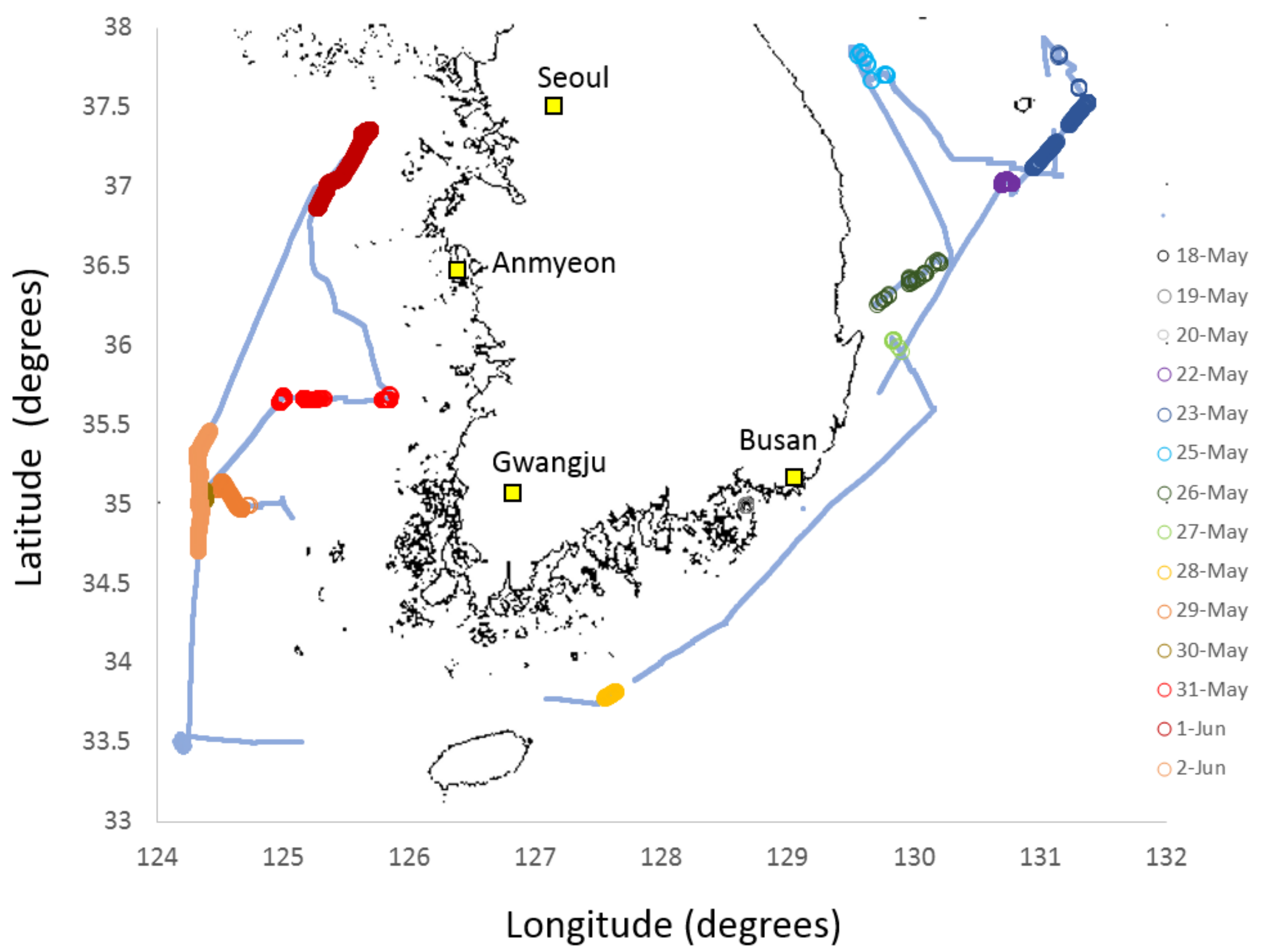
2.1. Study Region
2.2. Measurements of Total Column Trace Gases
2.3. HYSPLIT Trajectory Generation
3. Results and Discussion
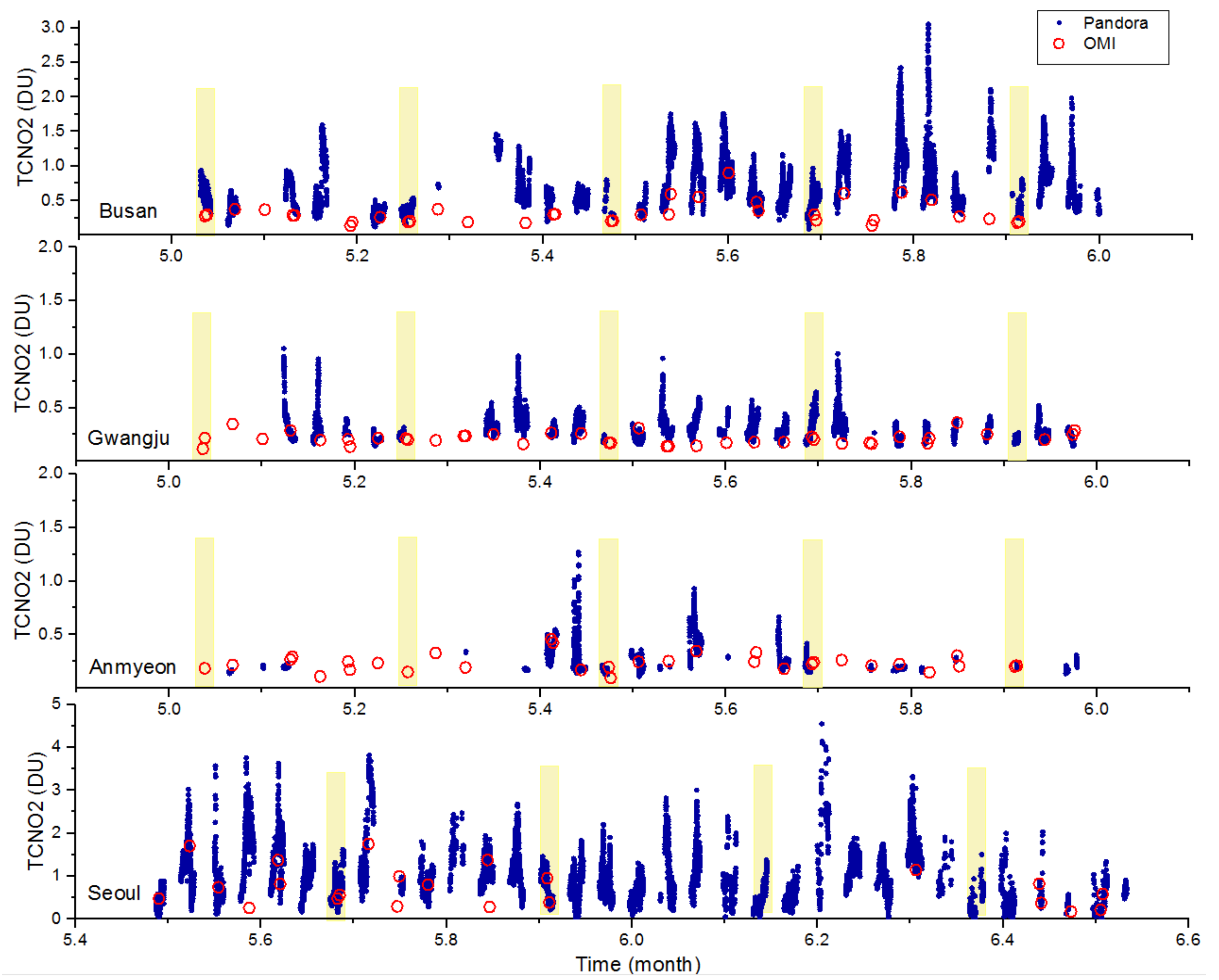
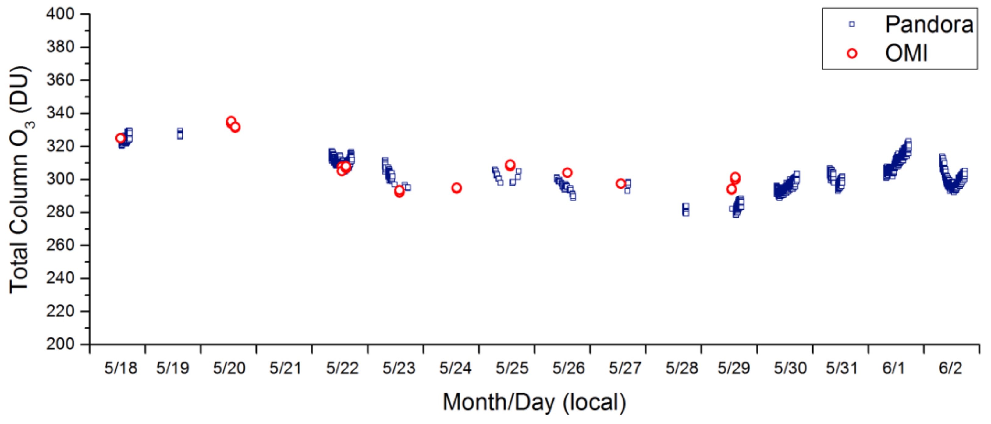
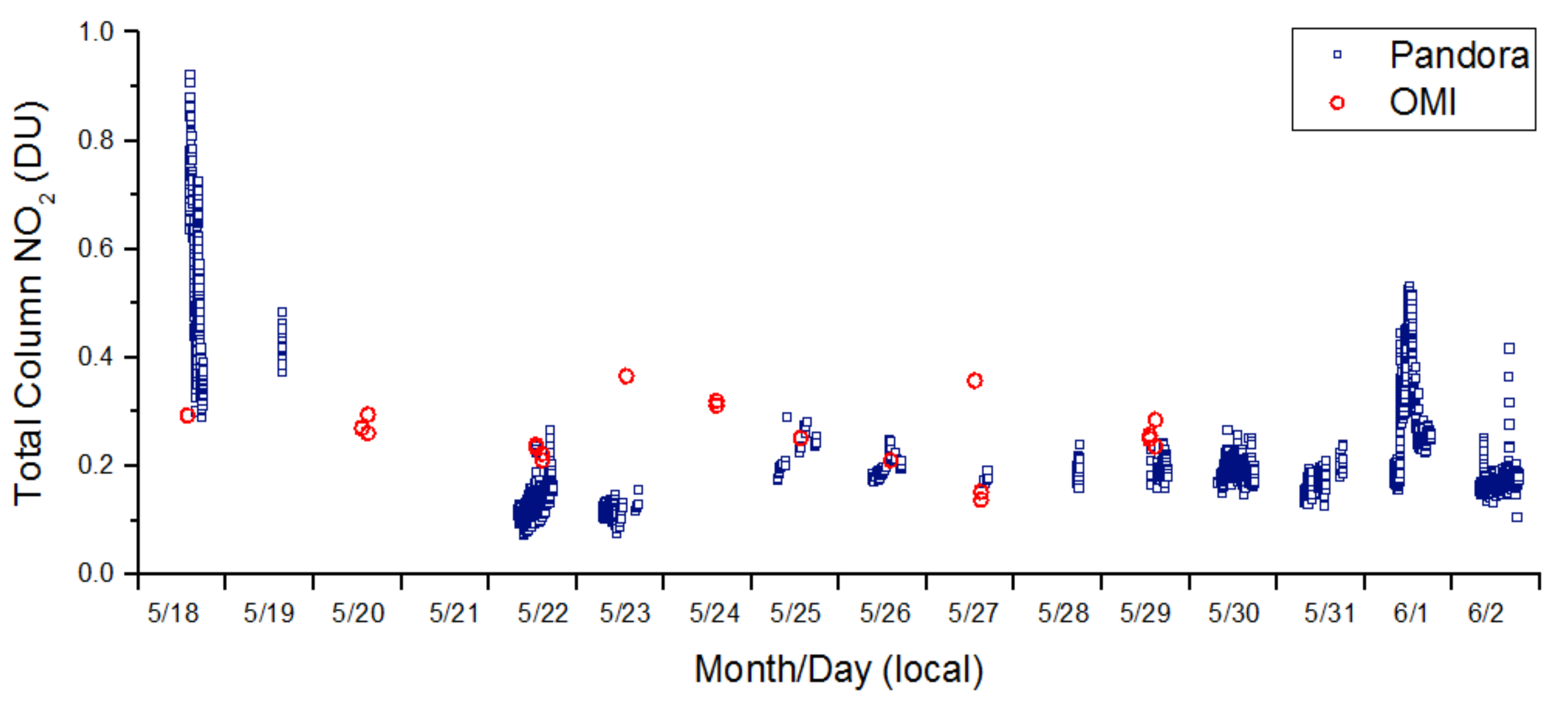
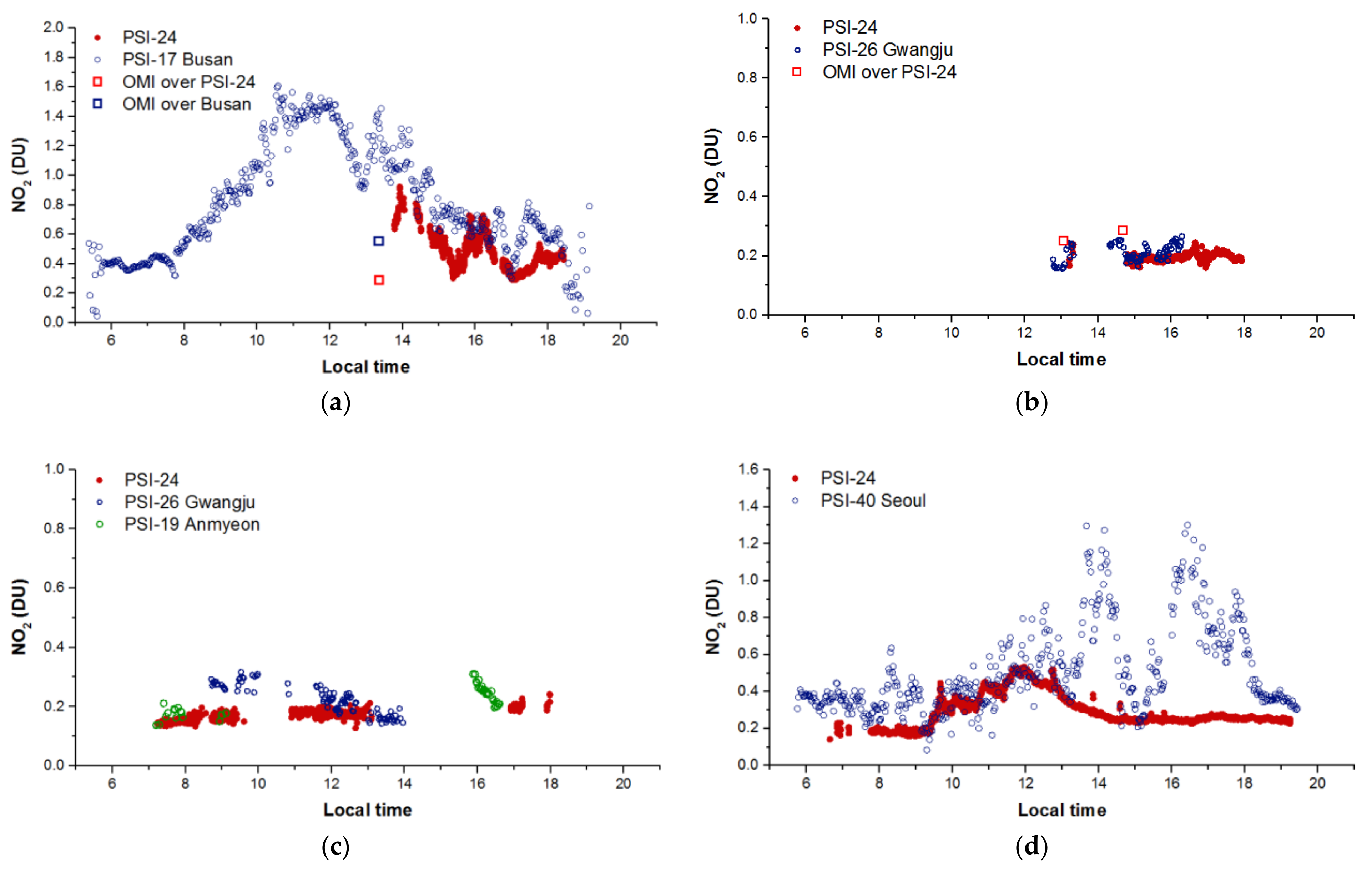
3.1. NO2 and O3 Dynamics over South Korean Coastal Land Sites
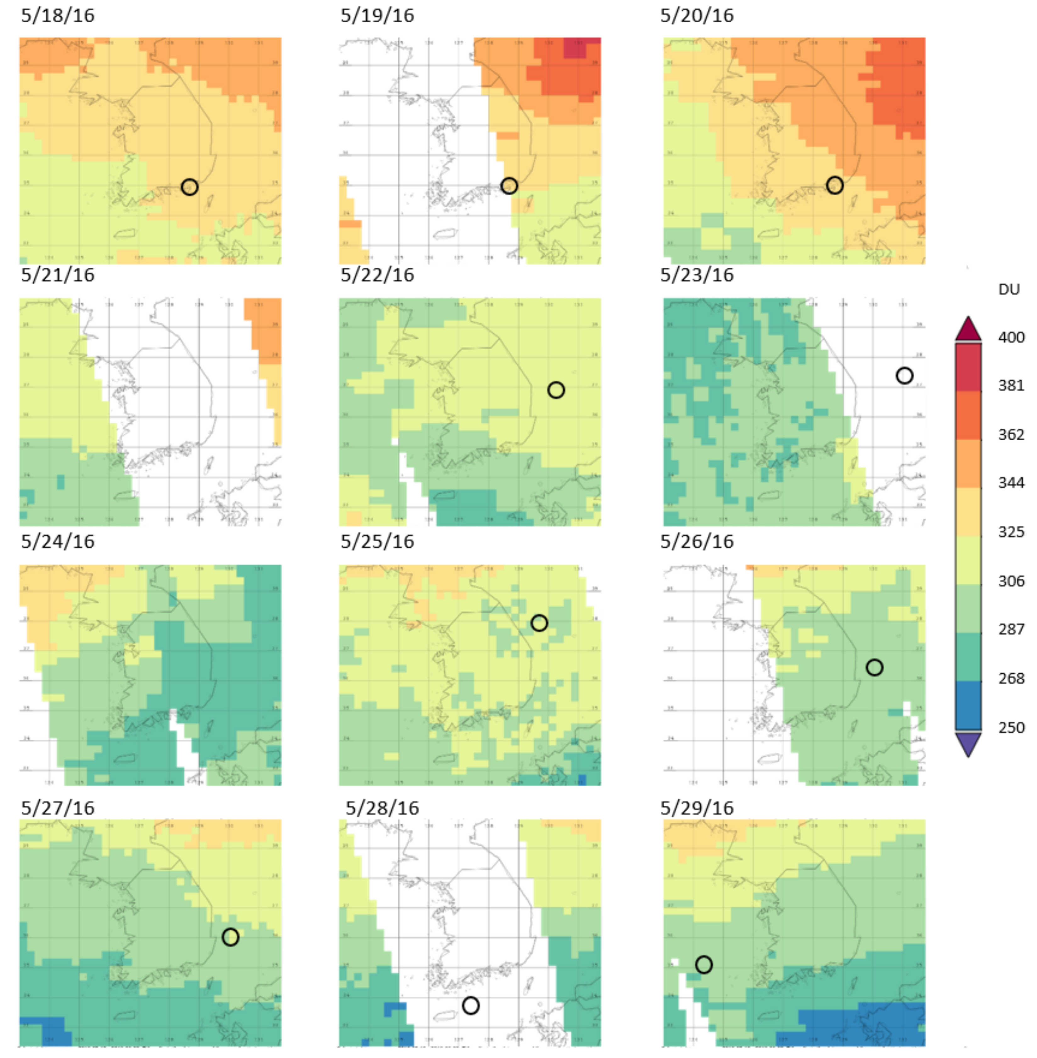
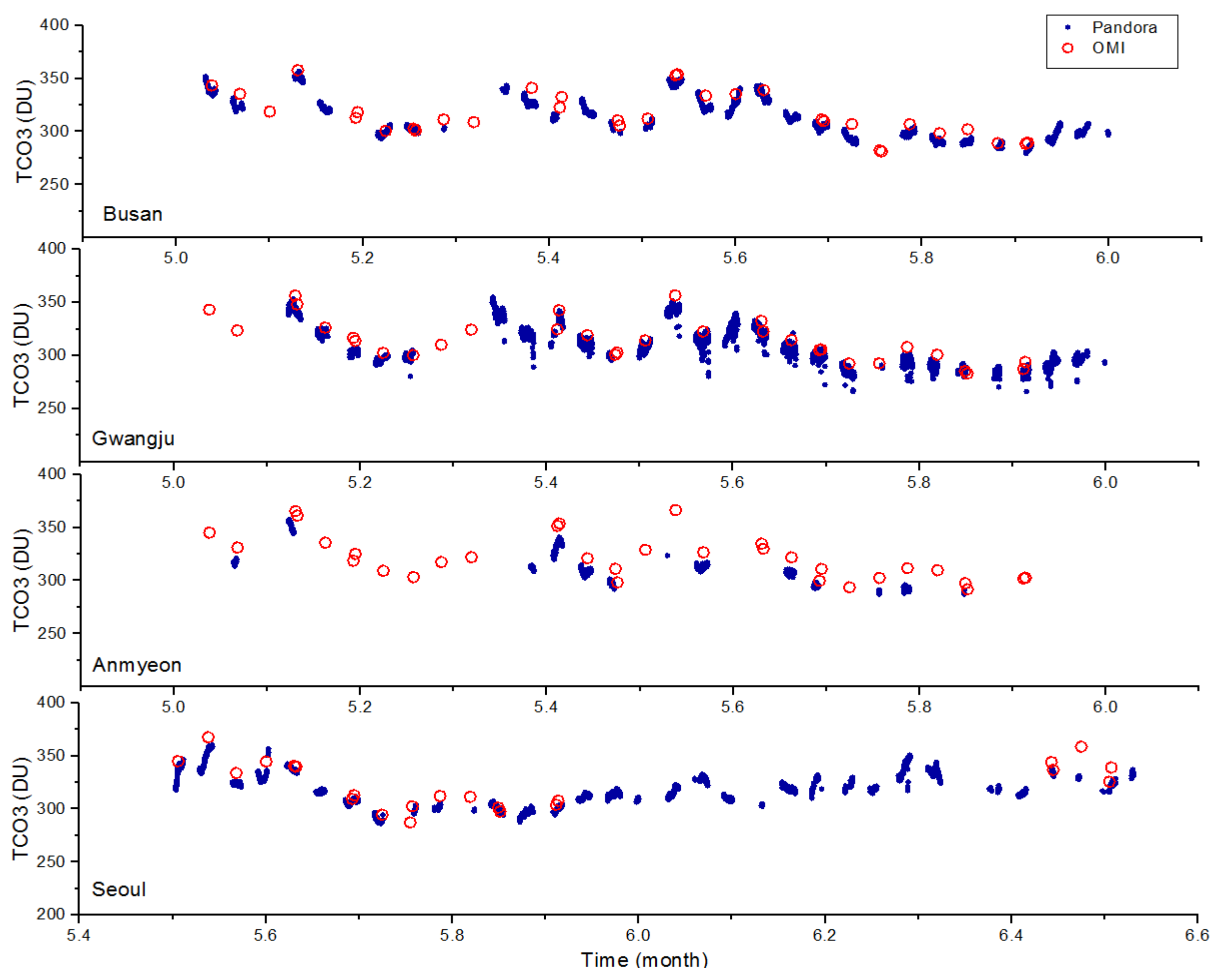
3.2. NO2 and O3 Dynamics Over the South Korean Coastal Waters
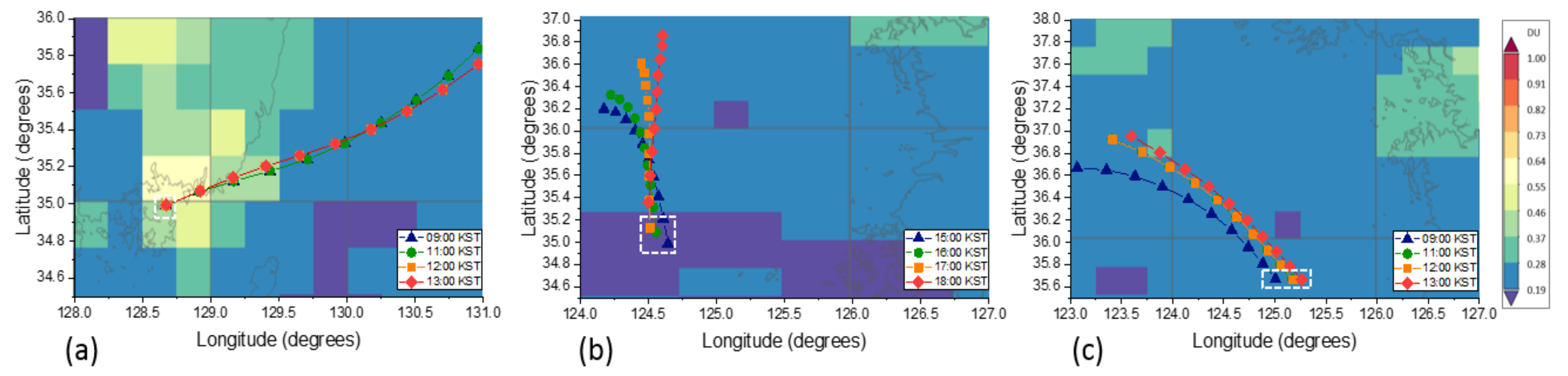
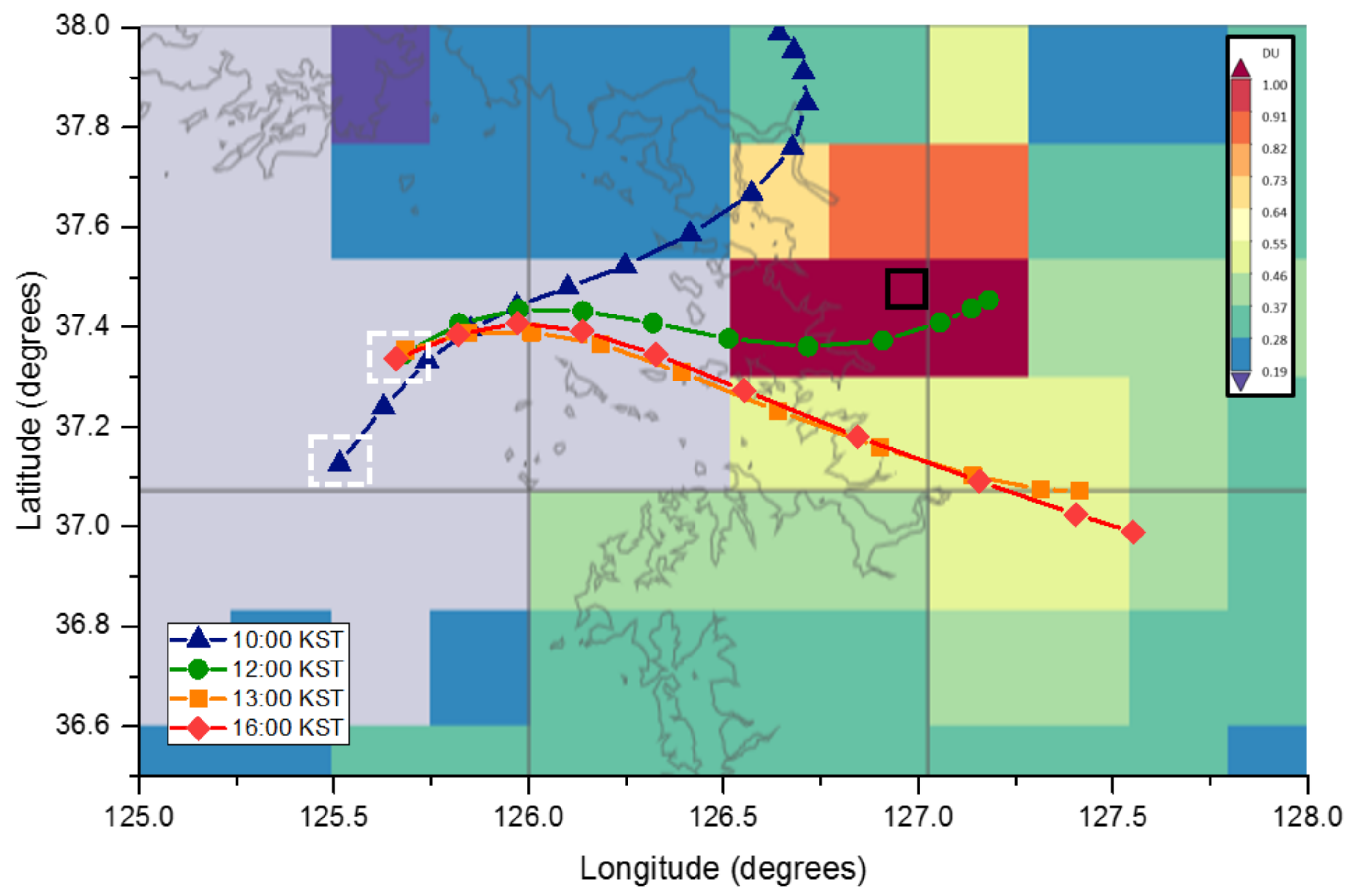
3.3. Back-Trajectories of Atmospheric Pollution Plumes
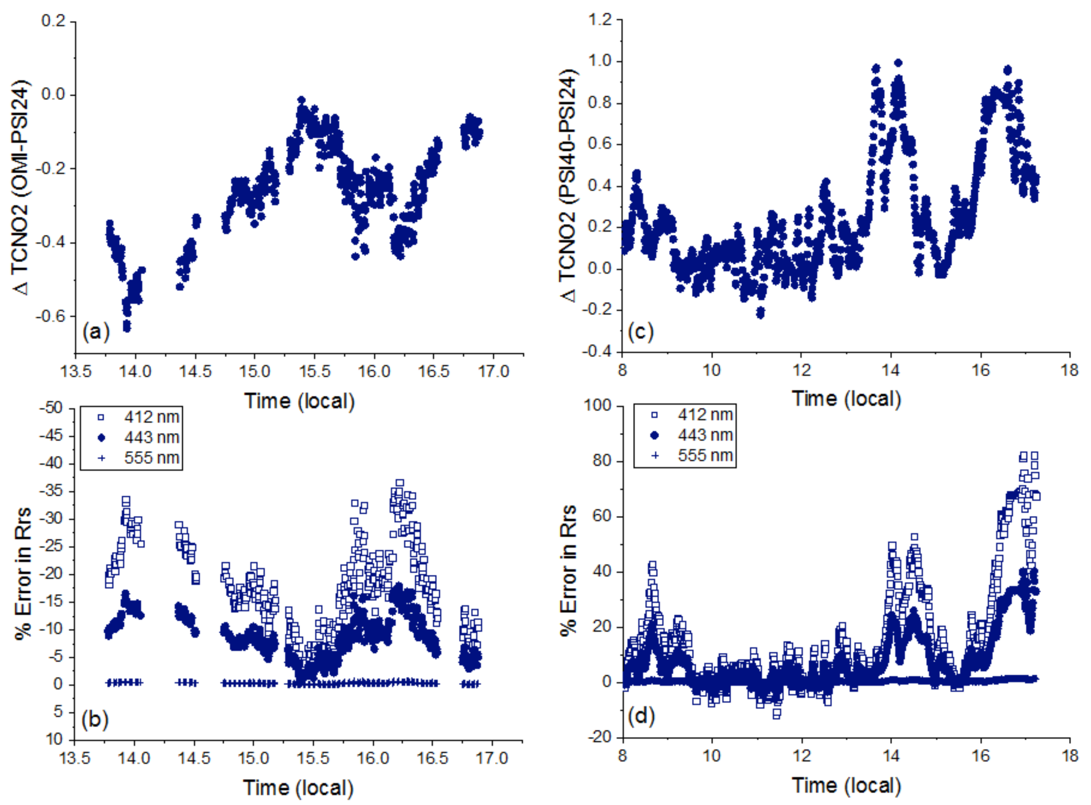
3.4. Implications of TCNO2 Variability for Remote Sensing of Ocean Color Dynamics
4. Conclusions
Author Contributions
Funding
Acknowledgments
Conflicts of Interest
References
- Herman, J.; Cede, A.; Spinei, E.; Mount, G.; Tzortziou, M.; Abuhassan, N. NO2 Column Amounts from Ground-based Pandora and MFDOAS Spectrometers using the Direct-Sun DOAS Technique: Intercomparisons and Application to OMI Validation. JGR Atmos. 2009, 114. [Google Scholar] [CrossRef]
- Tzortziou, M.; Herman, J.R.; Cede, A.; Loughner, C.P.; Abuhassan, N.; Naik, S. Spatial and temporal variability of ozone and nitrogen dioxide over a major urban estuarine ecosystem. J. Atmos. Chem. 2013. [Google Scholar] [CrossRef]
- Goldberg, D.L.; Loughner, C.P.; Tzortziou, M.; Stehr, J.W.; Pickering, K.E.; Marufu, L.T.; Dickerson, R.R. Higher surface ozone concentrations over the Chesapeake Bay than over the adjacent land: Observations and models from the DISCOVER-AQ and CBODAQ campaigns. Atmos. Environ. 2014, 84, 9–19. [Google Scholar] [CrossRef]
- Loughner, C.P.; Tzortziou, M.; Shroder, S.; Pickering, K.E. Enhanced dry deposition of nitrogen pollution near coastlines: A case study covering the Chesapeake Bay estuary and Atlantic Ocean coastline. J. Geophys. Res. Atmos. 2016, 121, 14–221. [Google Scholar] [CrossRef]
- Tie, X.; Geng, F.; Peng, L.; Gao, W.; Zhao, C. Measurement and modeling of O3 variability in Shanghai, China: Application of the WRF-Chem model. Atmos. Environ. 2009, 43, 4289–4302. [Google Scholar] [CrossRef]
- Kanakidou, M.; Mihalopoulos, N.; Kindap, T.; Im, U.; Vrekoussis, M.; Dermitzaki, E.; Gerasopoulos, E.; Unal, A.; Kocak, M.; Markakis, K.; et al. Megacities as hot spots of air pollution in the East Mediterranean. Atmos. Environ. 2011, 45, 1223–1235. [Google Scholar] [CrossRef]
- Von Glasow, R.; Jickells, T.D.; Baklanov, A.; Carmichael, G.R.; Church, T.M.; Gallardo, L.; Hughes, C.; Kanakidou, M.; Liss, P.S.; Mee, L.; et al. Megacities and large urban agglomerations in the coastal zone: Interactions between atmosphere, land, and marine ecosystems. Ambio 2013, 42, 13–28. [Google Scholar] [CrossRef] [PubMed]
- Stauffer, R.; Thompson, A.; Martins, D.K.; Clark, R.D.; Loughner, C.P.; Delgado, R.; Berkoff, T.A.; Gluth, E.C.; Dickerson, R.R.; Stehr, J.W.; et al. Bay Breeze Influence on Surface Ozone at Edgewood, MD, during July 2011. J. Atmos. Chem. 2012. [Google Scholar] [CrossRef] [PubMed]
- Loughner, C.P.; Tzortziou, M.; Follette-Cook, M.; Pickering, K.E.; Goldberg, D.; Satam, C.; Weinheimer, A.; Crawford, J.H.; Knapp, D.J.; Montzka, D.D.; et al. Impact of bay breeze circulations on surface air quality and boundary layer export. J. Appl. Meteorol. Climatol. 2014, 53, 1697–1713. [Google Scholar] [CrossRef]
- Ahmad, Z.; McClain, C.R.; Herman, J.R.; Franz, B.A.; Kwiatkowska, E.J.; Robinson, W.D.; Bucsela, E.J.; Tzortziou, M. Atmospheric correction for NO2 absorption in retrieving water-leaving reflectances from the SeaWiFS and MODIS measurements. Appl. Opt. 2007, 46, 6504–6512. [Google Scholar] [CrossRef] [PubMed]
- Tzortziou, M.; Herman, J.R.; Cede, A.; Abuhassan, N. High precision, absolute total column ozone measurements from the Pandora spectrometer system: Comparisons with data from a Brewer double monochromator and Aura OMI. J. Geophys. Res. 2012, 117, D16303. [Google Scholar] [CrossRef]
- Fishman, J.; Iraci, L.T.; Al-Saadi, J.; Chance, K.; Chavez, F.; Chin, M.; Coble, P.; Davis, C.; DiGiacomo, P.M.; Edwards, D.; et al. The United States’ Next Generation of Atmospheric Composition and Coastal Ecosystem Measurements: NASA’s Geostationary Coastal and Air Pollution Events (GEO APE) Mission. Bull. Am. Meteorol. Soc. 2012. [Google Scholar] [CrossRef]
- Salisbury, J.; Davis, C.; Erb, A.; Chuanmin, H.; Gatebe, C.; Jordan, C.; Lee, Z.; Mannino, A.; Mouw, C.B.; Schaaf, C.; et al. Coastal observations from a New Vantage Point: The NASA GEO-CAPE ocean mission. EOS Trans. J. 2016, 97. [Google Scholar] [CrossRef]
- Mobley, C.D.; Werdell, J.; Franz, B.; Ahmad, Z.; Bailey, S. Atmospheric Correction for Satellite Ocean Color Radiometry; A Tutorial and Documentation NASA Ocean Biology Processing Group, NASA Goddard Space Flight Center: Greenbelt, MD, USA, 2016; pp. 1–73. [Google Scholar]
- O’Reilly, J.E.; Maritorena, S.; Siegel, D.A.; O’Brien, M.C.; Toole, D.; Mitchell, B.G.; Kahru, M.; Chavez, F.P.; Strutton, P.; Cota, G.F.; et al. Ocean Color Chlorophyll a Algorithms for SeaWiFS, OC2, and OC4: Version 4; SeaWiFS Postlaunch Calibration and Validation Analyses, Part 3, NASA Tech. Memo. 2000-206892; NASA Goddard Space Flight Center: Greenbelt, MD, USA, 2000; Volume 11. [Google Scholar]
- Carder, K.L.; Chen, F.R.; Lee, Z.; Hawes, S.K.; Cannizzaro, J.P. Case 2 Chlorophyll-a MODIS Ocean Science Team Algorithm Theoretical Basis Document; Version 6, ATBD; 2002. [Google Scholar]
- Mannino, A.; Russ, M.E.; Hooker, S.B. Algorithm development for satellite-derived distributions of DOC and CDOM in the U.S. Middle Atlantic Bight. J. Geophys. Res. 2008, C07051. [Google Scholar] [CrossRef]
- Cao, F.; Tzortziou, M.; Hu, C.; Mannino, A.; Fichot, C.G.; Del Vecchio, R.; Najjar, R.G.; Novak, M. Remote Sensing retrievals of colored dissolved organic matter and dissolved organic carbon dynamics in North American eutrophic estuaries and their margins. Remote Sens. Environ. 2018, 205, 151–165. [Google Scholar] [CrossRef]
- Tzortziou, M.; Herman, J.R.; Ahmad, Z.; Loughner, C.P.; Abuhassan, N.; Cede, A. Atmospheric NO2 Dynamics and Impact on Ocean Color Retrievals in Urban Nearshore Regions. J. Geophys. Res.-Oceans 2008, C07051. [Google Scholar] [CrossRef]
- Pehlevan, N.; Ahn, J.; Jordan, C.E.; Tzortziou, M. Measurement requirements of atmospheric parameters for diurnal remote-sensing reflectance products. In Proceedings of the Abstract # 315585, 2018 Ocean Sciences Meeting, Portland, Oregon, 11–16 February 2018. [Google Scholar]
- Al-Saadi, J.; Carmichael, G.; Crawford, J.; Emmons, L.; Kim, S.; Song, C.-K.; Chang, L.-S.; Lee, G.; Kim, J.; Park, R. KORUS-AQ: An International Cooperative Air Quality Field Study in Korea; White Paper; 2014. [Google Scholar]
- Akimoto, H. Global air quality and pollution. Science 2003, 302, 1716–1719. [Google Scholar] [CrossRef] [PubMed]
- Richter, A.; Burrows, J.P.; Nüß, H.; Granier, C.; Niemeier, U. Increase in tropospheric nitrogen dioxide over China observed from space (and Supplementary Discussion on: Error estimates for changes in tropospheric NO2 columns as derived from satellite measurements). Nature 2005, 437, 129–132. [Google Scholar] [CrossRef] [PubMed]
- Lin, J.; Pan, D.; Davis, S.J.; Zhang, Q.; He, K.; Wang, C.; Streets, D.G.; Wuebbles, D.J.; Guan, D. China’s international trade and air pollution in the United States. Proc. Natl. Acad. Sci. USA 2014, 111, 1736–1741. [Google Scholar] [CrossRef] [PubMed] [Green Version]
- Park, Y.; Ahn, Y.-H.; Salisbury, J.; Mannino, A.; The GEO-CAPE Ocean Color Science Working Group. Risk Reduction Measurements for GEO-CAPE: A US-Korea Joint Field Campaign (US-Korea JFC) in the East Sea and Yellow Sea; White Paper; 2016. [Google Scholar]
- Pandey, S.K.; Kim, K.H.; Chung, S.Y.; Cho, S.J.; Kim, M.Y.; Shon, Z.H. Long-term study of NOx behavior at urban roadside and background locations in Seoul, Korea. Atmos. Environ. 2008, 42, 607–622. [Google Scholar] [CrossRef]
- Guttikunda, S.K.; Tang, Y.; Charmichael, G.R.; Kurata, G.; Pan, L.; Streets, D.G.; Woo, J.-H.; Thongboonchoo, N.; Fried, A. Impacts of Asian megacity emissions on regional air quality during spring 2001. J. Geophys. Res. 2005, 110, D20301. [Google Scholar] [CrossRef]
- Herman, J.; Spinei, E.; Fried, A.; Kim, J.; Kim, J.; Kim, W.; Cede, A.; Abuhassan, N.; Segal-Rozenhaimer, M. NO2 and HCHO measurements in Korea from 2012 to 2016 from Pandora spectrometer instruments compared with OMI retrievals and with aircraft measurements during the KORUS-AQ campaign. Atmos. Meas. Tech. 2018, 11, 4583–4603. [Google Scholar] [CrossRef]
- Levelt, P.F.; van den Oord, G.H.; Dobber, M.R.; Malkki, A.; Visser, H.; de Vries, J.; Stammes, P.; Lundell, J.O.; Saari, H. The Ozone Monitoring Instrument. IEEE Trans. Geosci. Remote Sens. 2006, 44, 1093–1101. [Google Scholar] [CrossRef]
- Boersma, K.F.; Eskes, H.J.; Veefkind, J.P.; Brinksma, E.J.; van der A, R.J.; Sneep, M.; van den Oord, G.H.J.; Levelt, P.F.; Stammes, P.; Gleason, J.F.; et al. Near-real time retrieval of tropospheric NO2 from OMI. Atmos. Chem. Phys. 2007, 7, 2103–2118. [Google Scholar] [CrossRef]
- Lamsal, L.N.; Krotkov, N.A.; Celarier, E.A.; Swartz, W.H.; Pickering, K.E.; Bucsela, E.J.; Gleason, J.F.; Martin, R.V.; Philip, S.; Irie, H.; et al. Evaluation of OMI operational standard NO2 column retrievals using in situ and surface-based NO2 observations. Atmos. Chem. Phys. 2014, 14, 11587–11609. [Google Scholar] [CrossRef]
- Dobber, M.; Kleipool, Q.; Dirksen, R.; Levelt, P.; Jaross, G.; Taylor, S.; Kelly, T.; Flynn, L.; Leppelmeier, G.; Rozemeijer, N. Validation of Ozone Monitoring Instrument level 1b data products. J. Geophys. Res. 2008, 113, D15S06. [Google Scholar] [CrossRef]
- Draxler, R.R.; Hess, G.D. Description of the HYSPLIT_4 Modeling System; NOAA Tech. Memo. ERL ARL-224; NOAA Air Resources Laboratory: Silver Spring, MD, USA, 1997; 24p. [Google Scholar]
- Draxler, R.R.; Hess, G.D. An overview of the HYSPLIT_4 modeling system of trajectories, dispersion, and deposition. Aust. Meteor. Mag. 1998, 47, 295–308. [Google Scholar]
- Challa, V.S.; Jayakumar, I.; Baham, J.M.; Hughes, R.; Patrick, C.; Young, J.; Rabbarison, M.; Swanier, S.; Hardy, M.G.; Anjaneyulu, Y. Sensitivity of atmospheric dispersion simulations by HYSPLIT to the meteorological predictions from a mesoscale model. Environ. Fluid Mech. 2008, 8, 367–387. [Google Scholar] [CrossRef]
- Wang, M.; Shi, W.; Jiang, L. Atmospheric correction using near-infrared bands for satellite ocean color data processing in the turbid western Pacific region. Opt. Express 2012, 20, 741–753. [Google Scholar] [CrossRef] [PubMed]
- Yerramilli, A.; Dodla, V.B.R.; Challa, V.S.; Myles, L.; Pendergrass, W.R.; Vogel, C.A.; Dasari, H.P.; Tuluri, F.; Baham, J.M.; Hughes, R.L.; et al. An integrated WRF/HYSPLIT modeling approach for the assessment of PM2.5 source regions over the Mississippi Gulf Coast region. Air Quality. Atmos. Health 2012, 5, 401–412. [Google Scholar] [CrossRef] [PubMed]
- Stein, A.F.; Draxler, R.R.; Rolph, G.D.; Stunder, B.J.; Cohen, M.D.; Ngan, F. NOAA’s HYSPLIT atmospheric transport and dispersion modeling system. Bull. Am. Meteorol. Soc. 2015, 96, 2059–2077. [Google Scholar] [CrossRef]
- Draxler, R.R. HYSPLIT4 User’s Guide; NOAA Tech. Memo. ERL ARL-230; NOAA Air Resources Laboratory: Silver Spring, MD, USA, 1999. [Google Scholar]
- Su, L.; Yuan, Z.; Fung, J.C.H.; Lau, A.K.H. A comparison of HYSPLIT backward trajectories generated from two GDAS datasets. Sci. Total Environ. 2015, 506–507, 527–537. [Google Scholar] [CrossRef] [PubMed]
- Kikuchi, K.; Wang, B. Global perspective of the quasi-biweekly oscillation. J. Clim. 2009, 22, 1340–1359. [Google Scholar] [CrossRef]
- Madhu, V. Madden Julian Oscillations in Total Column Ozone, Air Temperature and Surface Pressure Measured over Cochin during Summer Monsoon 2015. Open J. Mar. Sci. 2016, 6, 270–282. [Google Scholar] [CrossRef]
- Vasilkov, A.; Qin, W.; Krotkov, N.; Lamsal, L.; Spurr, R.; Haffner, D.; Joiner, J.; Yang, E.-S.; Marchenko, S. Accounting for the effects of surface BRDF on satellite cloud and trace-gas retrievals: A new approach based on geometry-dependent Lambertian equivalent reflectivity applied to OMI algorithms. Atmos. Meas. Tech. 2017, 10, 333–349. [Google Scholar] [CrossRef]
- Vasilkov, A.; Yang, E.-S.; Marchenko, S.; Qin, W.; Lamsal, L.; Joiner, J.; Krotkov, N.; Haffner, D.; Bhartia, P.K.; Spurr, R. A cloud algorithm based on the O2-O2 477 nm absorption band featuring an advanced spectral fitting method and the use of surface geometry-dependent Lambertian-equivalent reflectivity. Atmos. Meas. Tech. 2018, 11, 4093–4107. [Google Scholar] [CrossRef]
- Gitelson, A.A.; Schalles, J.F.; Hladik, C.M. Remote chlorophyll-a retrieval in turbid, productive estuaries: Chesapeake Bay case study. Remote Sens. Environ. 2007, 109, 464–472. [Google Scholar] [CrossRef]
- Tzortziou, M.; Subramaniam, A.; Herman, J.; Gallegos, C.; Neale, P.; Harding, L. Remote sensing reflectance and inherent optical properties in the Mid Chesapeake Bay. Estuarine Coast. Shelf Sci. 2007, 72, 16–32. [Google Scholar] [CrossRef]
- Le, C.; Hu, C.; Cannizzaro, J.; English, D.; Muller-Karger, F.; Lee, Z. Evaluation of chlorophyll-a remote sensing algorithm for an optically complex estuary. Remote Sens. Environ. 2013, 129, 75–89. [Google Scholar] [CrossRef]
- Torrecilla, E.; Stramski, D.; Reynolds, R.A.; Millán-Núñez, E.; Piera, J. Cluster analysis of hyperspectral optical data for discriminating phytoplankton pigment assemblages in the open ocean. Remote Sens. Environ. 2011, 115, 2578–2593. [Google Scholar] [CrossRef] [Green Version]


| Location | Lat | Lon | PSI | Measurement Period |
|---|---|---|---|---|
| Busan | 35.24° | 129.08° | PSI-17 | 07 April 2016–03 October 2016 |
| Gwangju | 35.23° | 126.84° | PSI-26 | 01 May 2015–17 October 2016 |
| Anmyeon | 36.54° | 126.33° | PSI-19 | 01 May 2016–06 June 2016 |
| Seoul | 37.56° | 126.93° | PSI-40 | 16 May 2016–15 October 2016 |
| OMI TCO3 | PSI TCO3 | %ΔTCO3 | OMI TCNO2 | PSI TCNO2 | %ΔTCNO2 | ||
|---|---|---|---|---|---|---|---|
| Busan | Average | 316 (±21) | 314 (±19) | 0.38% | 0.32 (±0.17) | 0.71 (±0.39) | −55.00% |
| 1 May–31 May 2016 | Range | 281–358 | 279–357 | 0.14–0.90 | 0.09-3.05 | ||
| Gwangju | Average | 315 (±20) | 311 (±19) | 1.17% | 0.20 (±0.05) | 0.31 (±0.13) | −37.01% |
| 1 May–31 May 2016 | Range | 283–357 | 266–355 | 0.11–0.30 | 0.14–1.05 | ||
| Anmyeon | Average | 322 (±21) | 315 (±17) | 2.15% | 0.24 (±0.08) | 0.27 (±0.14) | −11.37% |
| 1 May–31 May 2016 | Range | 292–366 | 287–357 | 0.1–0.46 | 0.11–1.27 | ||
| Seoul | Average | 323 (±22) | 320 (±15) | 1.15% | 0.75 (±0.48) | 1.01 (±0.64) | −25.45% |
| 16 May–16 June 2016 | Range | 287–367 | 286–360 | 0.17–1.75 | 0.01–5.78 |
© 2018 by the authors. Licensee MDPI, Basel, Switzerland. This article is an open access article distributed under the terms and conditions of the Creative Commons Attribution (CC BY) license (http://creativecommons.org/licenses/by/4.0/).
Share and Cite
Tzortziou, M.; Parker, O.; Lamb, B.; Herman, J.R.; Lamsal, L.; Stauffer, R.; Abuhassan, N. Atmospheric Trace Gas (NO2 and O3) Variability in South Korean Coastal Waters, and Implications for Remote Sensing of Coastal Ocean Color Dynamics. Remote Sens. 2018, 10, 1587. https://doi.org/10.3390/rs10101587
Tzortziou M, Parker O, Lamb B, Herman JR, Lamsal L, Stauffer R, Abuhassan N. Atmospheric Trace Gas (NO2 and O3) Variability in South Korean Coastal Waters, and Implications for Remote Sensing of Coastal Ocean Color Dynamics. Remote Sensing. 2018; 10(10):1587. https://doi.org/10.3390/rs10101587
Chicago/Turabian StyleTzortziou, Maria, Owen Parker, Brian Lamb, Jay R. Herman, Lok Lamsal, Ryan Stauffer, and Nader Abuhassan. 2018. "Atmospheric Trace Gas (NO2 and O3) Variability in South Korean Coastal Waters, and Implications for Remote Sensing of Coastal Ocean Color Dynamics" Remote Sensing 10, no. 10: 1587. https://doi.org/10.3390/rs10101587
APA StyleTzortziou, M., Parker, O., Lamb, B., Herman, J. R., Lamsal, L., Stauffer, R., & Abuhassan, N. (2018). Atmospheric Trace Gas (NO2 and O3) Variability in South Korean Coastal Waters, and Implications for Remote Sensing of Coastal Ocean Color Dynamics. Remote Sensing, 10(10), 1587. https://doi.org/10.3390/rs10101587