Article

Assessment of CO2 Emissions from Asphalt Pavement Maintenance Using a Life-Cycle Perspective: A Case Study of the Mexicali–San Felipe Highway

by
Diego Flores-Ruiz
,
Marco Montoya-Alcaraz
*,
Leonel García
,
José Manuel Gutiérrez-Moreno
,
Carlos Salazar-Briones
,
Julio Calderón-Ramírez
and
Alejandro Sánchez-Atondo
*
Civil Engineering Laboratory, Department of Civil Engineering, Engineering Faculty, Universidad Autónoma de Baja California, Mexicali 21280, Mexico
*
Authors to whom correspondence should be addressed.
Sustainability 2026, 18(9), 4461; https://doi.org/10.3390/su18094461
Submission received: 18 March 2026 / Revised: 18 April 2026 / Accepted: 27 April 2026 / Published: 1 May 2026
(This article belongs to the Special Issue Innovative and Sustainable Pavement Materials and Technologies)

Abstract

Maintaining asphalt pavements requires substantial quantities of materials and energy, which significantly contribute to greenhouse gas emissions in the road infrastructure sector. This study quantified the carbon dioxide equivalent (CO2e) emissions associated with a maintenance and rehabilitation plan for an asphalt pavement using a simplified life-cycle perspective integrated with the Highway Development and Management Model (HDM-4). The methodology combined HDM-4 to define a 35-year intervention plan (2022–2057) with CO2e emission factors for three quantified components: material production, transportation, and construction machinery operation. The approach was applied to a 7.8 km section of the Mexicali–San Felipe highway in Baja California, Mexico. The results indicate that the intervention plan generated approximately 2483.9 t CO2e over the 35-year analysis period. Reconstruction was the most carbon-intensive activity, accounting for 1890 t CO2e, while milling and overlay generated 292.15 t CO2e per direction. Material extraction and production were the dominant sources of emissions, contributing about 70% of the total emissions in milling and overlay and 60% in reconstruction; in the latter case, transportation also represented a substantial share (35%) due to long haul distances. These findings show that the proposed approach can identify the most emission-intensive activities and processes within pavement maintenance plans and provide quantitative environmental criteria to support more sustainable road management decisions.

1. Introduction

Population growth and global expansion have driven a significant increase in energy demand across sectors such as transportation, households, and industry. Given this growing demand, energy production and consumption are essential for societal development and economic improvement in any country [1]. Simultaneously, over the past three decades, global greenhouse gas (GHG) emissions have risen, albeit at a slightly slower rate. Since 2010, GHG emissions have been increasing, reaching approximately 5.9 ± 6.6 GtCO2e in 2019 [2].
In the road transport sector, the consumption of natural resources and energy is particularly high. The global transport network covers approximately 14 million km2 and is projected to grow by 60% from 2010 levels, potentially requiring the construction of an additional 25 million km of roads by 2050 [3,4,5]. According to reports from the International Energy Agency (IEA), CO2 emissions from fuel combustion in transportation continue to rise. For example, in 2020, global emissions fell by 8.3% (from 7737.8 to 7098.3 Mt) due to the COVID-19 pandemic. However, this reduction was brief because in 2022 they rebounded by 11.9%, reaching a record of 7941 Mt [6].
Despite their environmental impact, roads, bridges, and various transportation infrastructures are essential for a region or country to achieve growth. Not only does it facilitate the movement of people and goods, but it also enables access to services, education, and employment, acting as the backbone of economic and social development [7]. This growth is derived from a reduction in logistics expenses, which improves economic efficiency and attracts investments, promoting industrialization and urban growth [8,9]. In addition, various studies have specified that transport infrastructure projects promote economic growth and social welfare, thereby strengthening regional unity and expanding development opportunities in society [10,11,12,13,14].
Therefore, quantifying emissions from the construction of transport infrastructure has become increasingly important, as this practice serves as a basis for identifying the stages or processes with the greatest environmental impact and for establishing effective mitigation strategies to reduce polluting emissions. For this reason, calculating these emissions has become essential to minimize risks and move towards more sustainable development [15,16,17,18,19]. Thanks to these types of measurements, it is possible to detect critical pollution sources, select alternative, more environmentally friendly materials and techniques, and guide infrastructure planning toward a smaller carbon footprint [20,21]. To efficiently reduce carbon emissions in the construction sector, it is important to use accurate calculation methods that avoid misleading estimates and enable the design of reliable mitigation strategies [15,16]. Optimizing these measurement systems not only facilitates the path to carbon neutrality but also allows for the evaluation of the real impact of the implemented measures [16].
Although measuring the environmental impact of roads presents challenges, life cycle assessment (LCA) remains a useful framework for identifying the most relevant sources of emissions in pavement systems [22,23]. However, its application to pavements often involves considerable methodological complexity due to data requirements, assumptions, and modeling effort [24]. In this study, the life-cycle perspective is intentionally simplified to provide a practical assessment framework for pavement management. The analysis is limited to the quantification of CO2e emissions associated with the maintenance and rehabilitation plan, considering only material production, material transportation, and construction machinery operation. Accordingly, the approach excludes use-phase emissions and other environmental impact categories beyond climate change.
Based on this scope, this study proposes a simplified life-cycle approach that integrates the HDM-4 pavement management model with emission factors for materials, transportation, and construction machinery to quantify CO2e emissions associated with pavement maintenance and rehabilitation plans. The approach is then applied to a 7.8 km section of the Mexicali–San Felipe highway in Baja California, Mexico, as a case study to examine its applicability under local road conditions.

2. Background

Previous studies have applied LCA to assess the environmental impacts of asphalt pavements, accounting for their life-cycle stages. Likewise, the existing literature indicates that, to obtain robust and comparable results, it is essential to clearly and precisely define the system boundaries, appropriately select the functional unit (FU), and have access to reliable data inventories [25,26,27,28,29].
When LCA is implemented in pavements, most studies agree that the stage that contributes most to environmental impact is the extraction and production of materials for road construction. In other words, activities such as aggregate extraction (coarse and fine gravel), asphalt production, and hot-mix asphalt manufacturing generate the majority of greenhouse gas emissions throughout the pavement’s service life. For example, Liu et al. [30] indicate that heating aggregates is the most energy-intensive step in asphalt mix production, accounting for up to 97% of the total energy use. This high energy consumption is directly reflected in emissions, making this stage the main source of CO2 emissions within the pavement life cycle. Furthermore, recent research comparing traditional hot-mix asphalt (HMA) with warm-mix asphalt (WMA) has yielded important findings. The results of these comparisons confirm that producing asphalt at lower temperatures (using WMA technology) significantly reduces energy consumption and emissions generated during pavement manufacturing [31,32,33].
Furthermore, LCA-based mitigation strategies are driving the use of more sustainable materials and technologies in asphalt pavement construction. Several studies have shown that the use of recycled materials, such as reclaimed asphalt pavement (RAP), shredded tire rubber, and recycled polymers, as well as the adoption of lower-temperature asphalt mixtures, significantly reduces Global Warming Potential (GWP) emissions and energy consumption compared to traditional methods [34,35,36,37]. To summarize the current situation, a recent systematic review using the Preferred Reporting Items for Systematic Reviews and Meta-Analyses extension for Scoping Reviews (PRISMA-SCR) methodology identifies the main mitigation strategies in asphalt pavements and indicates that prioritizing well-planned conservation interventions, incorporating recycled materials, and optimizing construction processes represent key actions to reduce the environmental impact of the road sector [38].
In addition, over time, the literature has increasingly emphasized the role of pavement maintenance and rehabilitation throughout its lifespan. For example, Ma et al. [39] demonstrate that implementing a well-planned maintenance program significantly reduces a road’s overall carbon footprint. The key to this finding lies in preventing serious damage to the pavement surface. This is achieved by promptly addressing minor deterioration, thereby avoiding major repairs that consume significant energy and materials and consequently generate higher emissions. Complementing previous research, Zhang et al. [20] and Wang et al. [40] employ LCA methodologies to quantify emissions associated with specific maintenance interventions. Their findings indicate that the composition and thickness of structural layers, together with the type and quantity of materials used, are the primary drivers of environmental impact in road maintenance operations. Consequently, high-intensity interventions—such as full-depth reconstruction or complete resurfacing—account for the largest share of greenhouse gas emissions. On the other hand, routine maintenance, such as pothole repair or crack sealing, has a lower individual impact, but its effects accumulate year after year, also contributing to the overall environmental footprint of the road [26,41].
Therefore, integrating pavement management and performance models with a life-cycle approach has enabled more realistic and applicable evaluations. Recent studies have employed tools such as the HDM-4 model to simulate road deterioration, plan maintenance interventions, and, in some cases, determine fuel consumption and emissions generated by vehicles traveling on a given road segment [42,43,44]. In this way, it has been demonstrated that road conservation strategies can not only be evaluated but also optimized from a life cycle perspective, combining management models with specific emissions data associated with materials, transportation, and machinery used in construction [20,45]. Despite the advances reported in the literature, it remains necessary to develop studies that accurately measure the emissions produced by road maintenance programs on real sections, considering the specific conditions of vehicular traffic, climate, geometry, and the current state of the analyzed section.
In this context, several studies have indicated that incorporating environmental indicators based on LCA represents a significant advance for infrastructure management. This approach not only rigorously quantifies environmental impacts but also enriches the decision-making process. By including criteria such as greenhouse gas emissions in the evaluation of maintenance and rehabilitation alternatives, an objective comparison between different intervention scenarios is enabled, allowing for the prioritization of more sustainable strategies throughout the entire life cycle of roads [25,46,47].

3. Materials and Methods

3.1. Study Area

The study area is located in the state of Baja California, Mexico, within the municipality of Mexicali, on Federal Highway No. 5 Mexicali–San Felipe (Route MEX-005, code 02096). The analyzed section extends from kilometer marker 6 + 000 to 13 + 800, for a total length of 7.8 km (Figure 1).
The Mexicali–San Felipe highway is a 193.1 km strategic axis connecting the state capital with the coast of the Sea of Cortez. Historically, it has played a key role in the development of the region’s fishing and tourism, in addition to serving as a fundamental route for communication between cities, ports, the border with the United States of America (USA), and various tourist destinations.
The road is classified as a federal highway and has two lanes in each direction, a shoulder, and a median. This section was selected for its importance within the state highway network and the volume of traffic it carries, including a significant proportion of heavy vehicles. These conditions, combined with the region’s environmental characteristics, accelerate pavement wear and necessitate a maintenance plan to ensure proper performance throughout its lifespan.

3.2. Analysis Methodology

The methodology adopted in this study focuses on quantifying carbon dioxide emissions associated with the various asphalt pavement maintenance and rehabilitation activities required to preserve an adequate level of service for users. Each intervention involves material and energy consumption, leading to emissions generated during the stages of raw material extraction, material production, transportation, and on-site construction.
To develop the intervention plan, HDM-4 software (version 1.3) was used as the pavement management tool to simulate pavement performance and define maintenance and rehabilitation activities throughout the analysis period. Its selection was based on its broad application in previous pavement management and road deterioration studies. In this study, HDM-4 was applied using the available local input data for the analyzed section, including traffic, pavement condition, geometry, and environmental context. However, no independent local calibration or validation of the deterioration model was conducted for this specific road segment, and no historical local validation of previous HDM-4 forecasts against observed pavement deterioration was available for the case study. Therefore, the intervention plan should be interpreted as a planning-based scenario derived from the adopted model structure and input data rather than as a fully locally calibrated prediction of pavement deterioration over time.
Accordingly, the intervention schedule generated by HDM-4 serves as the foundation for the subsequent estimation of emissions associated with material consumption and energy use in each programmed activity aimed at maintaining pavement condition. In this study, HDM-4 was used only to define the intervention plan over the analysis period, whereas the CO2e quantification was performed independently using literature-based emission factors applied to the materials, transportation, and machinery requirements of each intervention.
In this context, Figure 2 illustrates the proposed methodological framework for quantifying emissions derived from the pavement intervention plan.
As shown in Figure 2, the computational workflow was implemented in four sequential stages. First, local input data related to traffic, pavement condition, geometry, and environmental context were compiled and entered into HDM-4 to generate the maintenance and rehabilitation plan for the analysis period. Second, the intervention schedule obtained from HDM-4 was used to determine the quantities of materials, transport requirements, and construction equipment associated with each activity. Third, emissions were calculated separately for material production, transportation, and machinery operation using Equations (2), (3), and (4), respectively. Finally, total emissions for each intervention were obtained by summing these components according to Equation (1), and the resulting values were then compared by activity and by emission source. To make this workflow more explicit, Table 1 presents the correspondence between each block of the methodological framework shown in Figure 2 and the associated calculation procedure.

3.3. Input Data

Based on the above, the intervention-plan analysis required the characterization of the study section in terms of traffic, pavement structure, geometry, current condition, and environmental context.
  • Environmental and geographic conditions of the road segment, which influence pavement deterioration mechanisms and long-term performance.
  • Annual Average Daily Traffic (AADT), including vehicle fleet composition and projected traffic growth, is a critical factor for estimating traffic loading and structural demand.
  • Geometric characteristics of the study segment, such as segment length and width, number of lanes, and the structural configuration of pavement layers, including the subbase, base course, and asphalt surface layer.
  • Current pavement condition, determined using several performance indicators, including the International Roughness Index (IRI), surface deflection, total cracked area, and rut depth.
  • The study segment is located in northwestern Mexico, within the municipality of Mexicali, Baja California. This region is characterized by an extreme arid climate, with summer temperatures frequently exceeding 45 °C and winter temperatures occasionally dropping below 5 °C. These conditions induce significant variability in the mechanical and rheological behavior of asphalt materials.
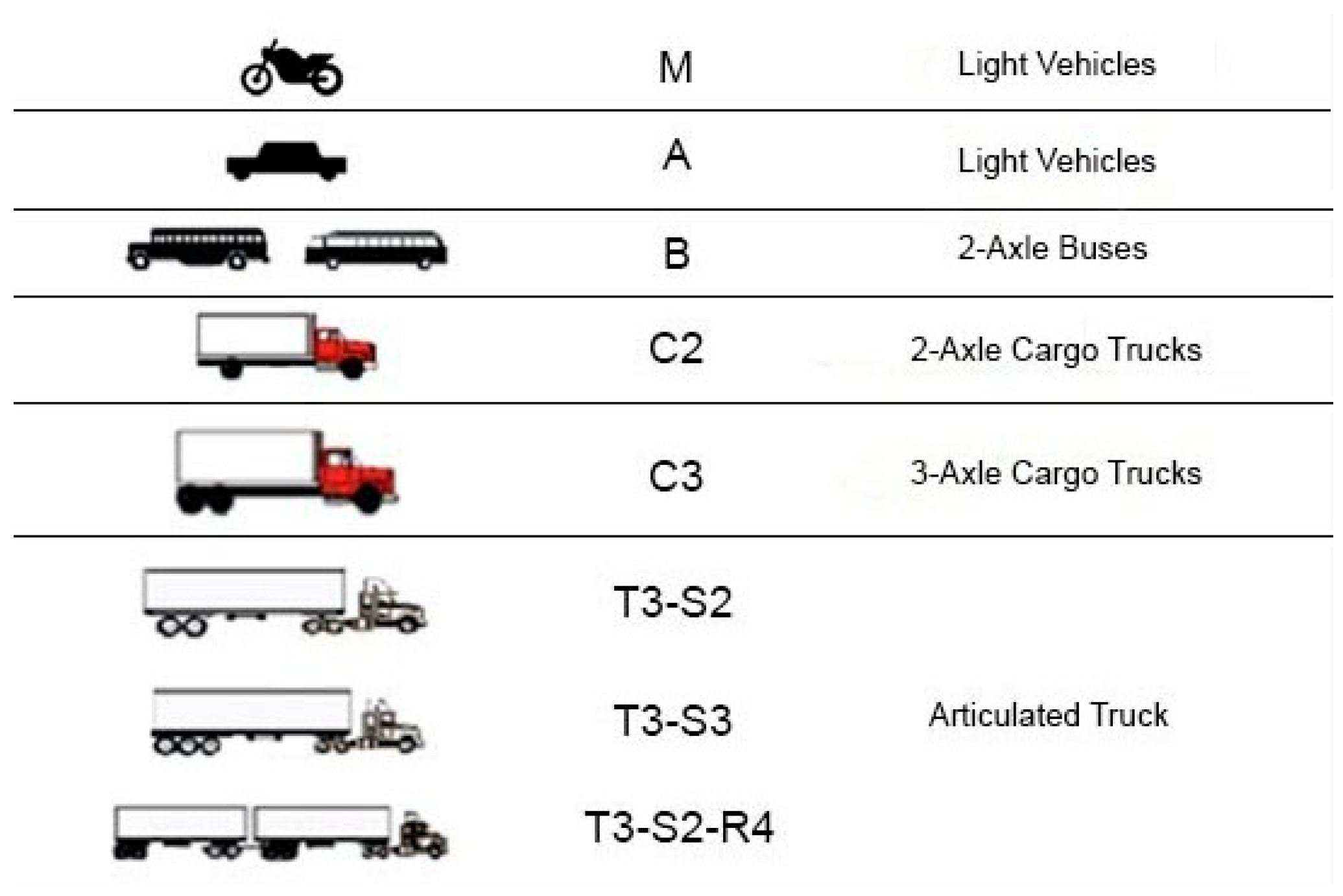
Regarding the traffic demand along the roadway, Annual Average Daily Traffic (AADT) data were obtained from the database of the Secretariat of Infrastructure, Communications, and Transportation (SICT) [48]. Vehicle fleet composition is the relative proportion of different vehicle types traveling on a roadway and is a fundamental factor for characterizing traffic demand and estimating pavement deterioration processes [49]. For this analysis, both the AADT and vehicle class distribution were determined based on the standard configuration of major vehicle types operating on the national road network, as published in the official Mexican standard issued by SICT [50] (Figure 3). In the Mexican vehicle classification system, T3S2 refers to a tractor-semitrailer configuration with a three-axle tractor and a two-axle semitrailer, whereas T3S3 refers to a configuration with a three-axle tractor and a three-axle semitrailer. Thus, the distinction between the two classes is associated with the number of axles in the articulated freight vehicle configuration.
Historical AADT records for the period 2011–2022 were also used to estimate the annual traffic growth rate for the analysis period. Pandemic years were excluded from this estimation in order to avoid distortions in the traffic trend. Based on the available historical series, direction-specific baseline annual traffic growth rates were adopted for the HDM-4 analysis: 3.6% for the Mexicali–San Felipe direction and 2.1% for the San Felipe–Mexicali direction. In this context, Table 2 presents the average annual daily traffic for both lanes and the vehicle classification for the road segment. Type A vehicles (light vehicles) represent 78.9% in the Mexicali-to-San Felipe direction and 79.4% in the opposite direction.
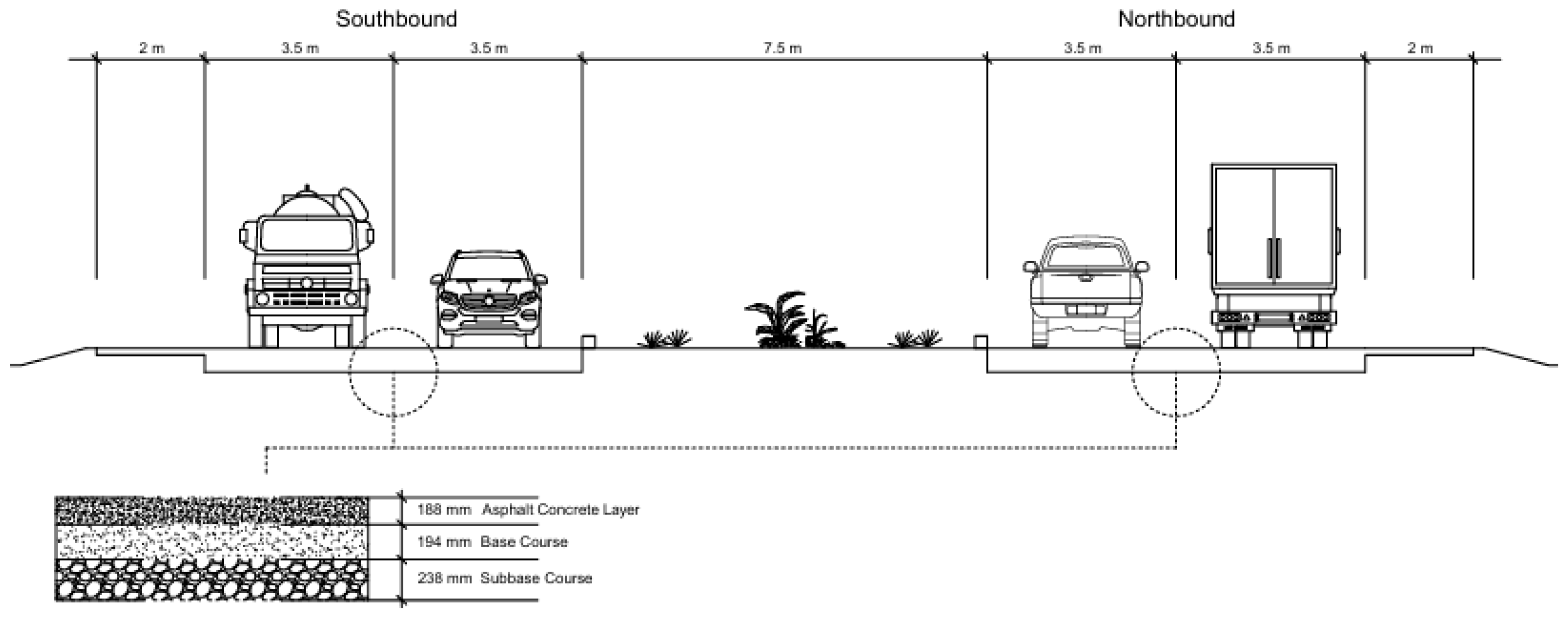
The study section is 7.8 km long and consists of two traffic lanes, each 3.5 m wide, with a 2 m side shoulder in each direction and a 7.5 m central median. The pavement structure consists of three main layers: a 23.8 cm granular subbase, a 19.4 cm granular base, and an 18.8 cm asphalt surface course, which is a bituminous mix that provides the riding surface (Figure 4).
The structural and functional condition of the pavement was assessed using indicators reported by the SICT for the years 2021 and 2022. The results indicate an average surface deflection of 0.46 mm, measured under a load of 700 kPa, reflecting the structural capacity of the study segment. Regarding surface condition, the IRI was 2.48 m/km in the Mexicali–San Felipe direction and 2.78 m/km in the opposite direction, indicating an acceptable level of service. The mean rut depth was 12.27 mm and 12.11 mm, respectively, while the total cracked area reached 26% in one direction and 8.4% in the other. These results reveal directional differences in pavement deterioration associated with traffic loading patterns (Table 3).
To improve transparency in the application of HDM-4, Table 4 summarizes the key numerical parameters explicitly highlighted in the present study for generating the intervention plan, particularly those related to traffic demand and its representation within the model. In the present study, the model was parameterized using the base-year AADT, the projected traffic growth rate, and the vehicle fleet configuration/classification according to NOM-012-SCT-2-2017 [50]. Equivalent single axle loads (ESALs) were not entered as an independent input parameter, since traffic loading was represented through these traffic variables within the HDM-4 framework. For climatic characterization, the “subtropical hot/semi-arid” category was selected as the closest available option to the environmental conditions of Mexicali, Baja California.
This climatic representation was used as the closest available environmental approximation within HDM-4 for the study area. However, detailed local variables such as precipitation amount and frequency, wetting-drying cycles, heating-cooling cycles, and traffic intensity under those specific climatic conditions were not introduced as independent input parameters in the present analysis.

3.4. Data Processing

Based on the input data (environmental conditions, traffic, geometry, and current pavement condition), an intervention plan was generated using HDM-4 software, which simulates pavement performance over time in relation to initial conditions, traffic, and applied maintenance standards.
According to standard N·CSV·CAR·1·03·004/21 [51], pavement condition can be classified based on IRI values into good, fair, and poor service levels. In this study, these criteria were used as the basis for defining the IRI thresholds shown in Table 5. Accordingly, an IRI value of 3.5 m/km was adopted as the threshold for periodic maintenance because it corresponds to the upper limit of the fair condition range. Likewise, an IRI value of 4.5 m/km was adopted as the reconstruction threshold in order to represent a more advanced deterioration level requiring structural intervention.
In addition, thresholds of 25 potholes per kilometer and 10% cracked area were adopted as operational criteria to trigger routine maintenance actions such as patching and crack sealing. These values were not taken directly from a design standard but were defined as practical intervention thresholds consistent with routine pavement maintenance practice commonly applied by road agencies, with the aim of identifying early surface deterioration conditions that justify preventive action before the pavement reaches more severe states requiring major rehabilitation.
After defining the threshold values, maintenance standards were established to generate the intervention plan (Table 6). These standards allow HDM-4 to select, for each analysis year, between routine maintenance, periodic maintenance, or reconstruction actions. Separate specifications were also defined for milling and resurfacing interventions and for reconstruction based on IRI thresholds, ensuring that once a milling and resurfacing treatment was applied, it was excluded from subsequent intervention selection.
According to these standards, HDM-4 selects the most appropriate intervention each year: routine maintenance (pothole patching or crack sealing), periodic conservation (milling and resurfacing), or reconstruction. After the information-gathering process, the conservation scenario was established for a 35-year analysis period (2022–2057). In this study, the intervention schedule was configured as a rule-based maintenance and rehabilitation scenario over the analysis horizon, including routine maintenance, a single milling-and-overlay action per direction, and major rehabilitation when pavement condition reached a severe deterioration level. Therefore, the resulting plan should be interpreted as a planning-based scenario used to quantify the CO2e emissions associated with the main intervention types considered in the study, rather than as an optimization exercise aimed at maintaining the pavement within the good-to-fair range throughout the entire analysis period.
It should be noted that the intervention plan generated in this study was defined at the road-section level as a planning scenario to maintain pavement serviceability over time, based primarily on condition thresholds such as IRI. Therefore, the proposed interventions were not spatially allocated to specific chainages or sub-sections of the analyzed segment but rather represent section-level maintenance and rehabilitation actions derived from the modeled pavement performance.
In accordance with the HDM-4 intervention plan, an inventory of inputs and resources required to carry out each pavement conservation and rehabilitation activity was compiled. This inventory is an essential component for the emissions analysis and is structured into three main categories: raw material production and extraction, material transportation, and construction operations.
The emissions generated by the consumption of materials required for each intervention activity (aggregate, asphalt binder, and HMA production) were estimated based on the specifications and volumes specified in HDM-4. To quantify the environmental emissions associated with material production, emission factors reported in the existing literature were used. These factors were selected because they represent production processes commonly considered in pavement life-cycle studies and provide a practical basis for estimating emissions when locally standardized factors are not available. However, it is recognized that their absolute values may vary according to regional conditions such as the energy mix, fuel sources, industrial efficiency, and production technology. Therefore, the factors adopted in this study should be interpreted as reference values used to estimate the relative contribution of the main material-related processes in the case study, rather than as exact Mexico-specific coefficients. The emission factors considered in this study are presented in Table 7.
To estimate emissions associated with material transportation, the following logistics routes were considered:
  • Raw materials transported from the quarry or refinery to the asphalt mixing plant.
  • Asphalt mixtures delivered from the mixing plant to the construction site.
  • Raw materials transported directly from the quarry or refinery to the construction site.
Vehicle fuel consumption was expressed in liters per kilometer traveled. Transportation-related emissions were estimated using a reference emission factor of 0.886 kg CO2e per kilometer traveled by a heavy-duty truck, as reported by Gialos et al. [54]. In the present study, this factor was applied to loaded trips associated with the delivery of materials required for each intervention activity. Return trips were not included in the calculation, since their loading condition depends on the logistics and operational practices of suppliers and transport companies and could not be defined consistently for the case study. Therefore, the transport-related results should be interpreted as a simplified estimate based on inbound material-hauling trips. Table 8 summarizes the transport distances considered between material supply locations and the construction site.
In the case of construction, which comprises the various activities required by the pavement maintenance plan, the different types of machinery necessary to carry out the designated work are considered. Furthermore, the energy consumption associated with machinery operation is established. To this end, the main equipment used for patching, crack sealing, milling, and reconstruction interventions was identified, along with the volumes of fuel used during their operation.
Energy consumption was estimated based on average fuel-consumption values reported in technical manuals and published literature, expressed in liters of diesel per hour of operation. These reference values were used because project-specific field measurements and detailed equipment utilization records were not available for the analyzed case study. Therefore, the machinery-related emissions should be interpreted as simplified estimates derived from representative average operating conditions rather than from direct on-site measurements. These values were multiplied by the number of working hours required for each intervention, based on the assumed equipment performance, to obtain the total fuel consumption per activity. The construction machinery considered in this study was defined based on equipment categories reported in previous pavement life-cycle studies and technical references, rather than on manufacturer-specific commercial models. Accordingly, the equipment listed in Table 9 represents functional construction equipment categories used to estimate diesel consumption and associated CO2e emissions.
Emission quantification was conducted in accordance with the guidelines established by the Intergovernmental Panel on Climate Change (IPCC, 2006) [57]. Emissions were expressed in kg CO2e using Global Warming Potential values over a 100-year time horizon (GWP100). Fuel consumption and material input data were used for this purpose and multiplied by their corresponding specific emission factors. In the present study, greenhouse gas emissions were not disaggregated by individual species (e.g., CO2, CH4, or N2O). Instead, the results were expressed as CO2e using literature-based emission factors under the GWP100 approach.
In accordance with the workflow presented in Figure 2, emissions were quantified independently for the three main components of the intervention plan: material production, transportation, and machinery operation. The calculation framework used in Equations (1)–(4) was not proposed as a new mathematical model but was adapted from activity-based emission accounting approaches reported in previous studies [39,58]. In particular, the transport-related formulation follows the general summation structure reported in Ref. [58], while the material- and machinery-related expressions were structured following summation-based emission formulations applied in pavement studies such as Ref. [39]. These components were estimated through Equations (2)–(4), and the total emissions were obtained by aggregating the corresponding CO2e contributions through Equation (1).
E C O 2 e = ( A   ×   E F )
where E C O 2 e represents the total carbon dioxide equivalent emissions [kg CO2e]; A denotes the activity level or inventory flow; and E F is the corresponding emission factor. The specific units of activity data and emission factors for each component are defined in Equations (2)–(4). Therefore, the intermediate results obtained from Equation (1) are expressed in kg CO2e and were later converted to t CO2e for reporting purposes.
Emissions associated with material production ( E m j ) were calculated as the sum of the quantities of each material ( M i ) used in the different intervention activities ( j ), multiplied by their respective emission factors ( E F i ), as expressed in Equation (2):
E m j = i ( M i   ×   E F i )
where i represents the material type; j represents the intervention activity; E m j is the emissions associated with material production [kg CO2e]; M i is the quantity of material i [t]; and E F i is the CO2e emission factor for material i [kg CO2e/t]. Therefore, the emissions estimated with Equation (2) are expressed in kg CO2e.
Similarly, emissions generated by material transportation ( E t j ) were calculated as the sum of the emissions associated with the transport of each material ( i ) from the aggregate quarry or asphalt plant to the construction site for the different intervention activities ( j ). This calculation considered the number of required trips ( V i ), the transport distance along each route ( D i ), and the emission factor corresponding to the transport vehicle ( E F veh ), as shown in Equation (3):
E t j = i ( V i × D i × E F veh )
where i represents the material type; j represents the intervention activity; E t j is the emissions associated with material transportation [kg CO2e]; V i is the number of loaded trips required to transport material i [number of trips]; D i is the transport distance for each route [km]; and E F v e h is the CO2e emission factor of the transport vehicle [kg CO2e/km]. Therefore, the emissions estimated with Equation (3) are expressed in kg CO2e.
Finally, emissions generated by construction equipment use ( E c j ) during construction activities ( j ) were estimated based on the fuel consumption of each equipment type ( i ). The calculation considered the total volume of fuel consumed by each piece of equipment ( L i ) and the corresponding emission factor ( E F i ), as expressed in Equation (4):
E c j = i ( L i × E F i )
where i represents the equipment type; j represents the intervention activity; E c j is the emissions associated with construction equipment use [kg CO2e]; L i is the total fuel consumption of equipment i [L]; and E F i is the CO2e emission factor associated with the consumption of one liter of fuel by equipment i [kg CO2e/L]. Therefore, the emissions estimated with Equation (4) are expressed in kg CO2e.

4. Results

4.1. Pavement Intervention Plan

The maintenance plan for the Mexicali–San Felipe highway section was generated using simulation software HDM-4, considering a 35-year horizon (2022–2057). This plan integrates routine, periodic, and major interventions to represent pavement serviceability evolution over the analysis period.
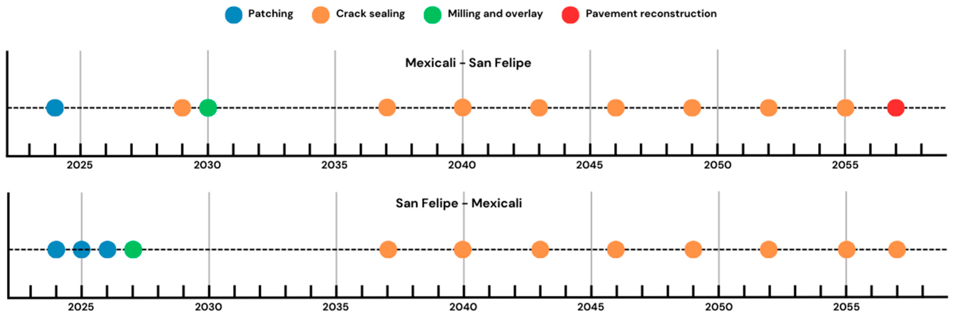
Scheduled activities include pothole repair, crack sealing, and milling and resurfacing in both traffic directions, while a major reconstruction was included only in the Mexicali–San Felipe direction at the end of the analysis period. Therefore, the intervention schedules differ between directions, reflecting the modeled deterioration path and the adopted intervention rules in each case. The frequency and type of intervention depend on established deterioration thresholds (IRI, cracking, number of potholes) and the volume of heavy traffic using the highway. The inclusion of reconstruction in one direction allowed the study to represent a major rehabilitation activity within the analysis horizon and to quantify its associated CO2e emissions.
Table 10 and Table 11 present the activity schedule, while Figure 5 illustrates the temporal distribution of the planned interventions.
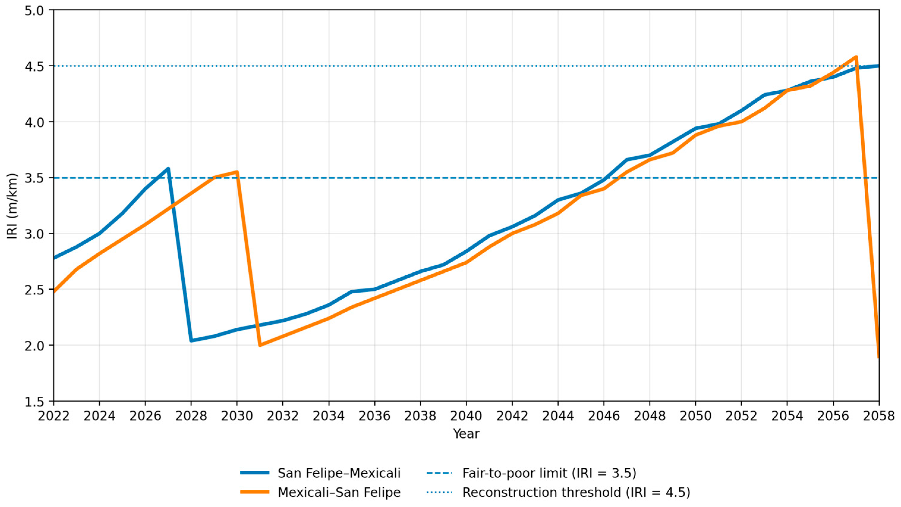
Figure 6 shows the modeled IRI evolution for both traffic directions under the adopted intervention scenario during the 2022–2057 analysis period. The curves illustrate the progressive increase in pavement roughness over time, as well as the effect of the programmed maintenance and rehabilitation actions on pavement serviceability. Routine interventions such as patching and crack sealing help control the progression of surface deterioration and delay the increase in IRI, whereas milling and overlay and major rehabilitation produce more noticeable reductions in roughness levels. The figure should be interpreted in relation to the serviceability thresholds adopted in the study, namely 2.5 m/km for the good-to-fair limit, 3.5 m/km for the fair-to-poor limit, and 4.5 m/km as the reconstruction threshold. These results should therefore be interpreted as the modeled roughness trajectory associated with the adopted intervention rules, rather than as evidence that the pavement remains continuously within the good-to-fair condition range throughout the full analysis period.

4.2. Emissions Generated by Each Activity

Based on the conservation plan generated by HDM-4, CO2e emissions were quantified for each type of intervention, distinguishing three components: material production, transportation, and on-site machinery. Table 12 presents the emissions generated by each type of activity included in the pavement conservation plan. The results correspond to the sum of emissions derived from material production, transportation, and machinery operation during each intervention.
It can be observed that the highest-impact activities (such as milling and resurfacing, and reconstruction) account for the majority of emissions, due to the high volume of materials used and the energy required for their execution. In contrast, routine interventions, such as patching and crack sealing, have considerably lower emissions, though their frequency cumulatively contributes to total projected emissions.
To improve comparability with other studies, the emissions associated with each intervention activity were also normalized by the analyzed section length (7.8 km) and are presented in Table 12 as t CO2e/km.
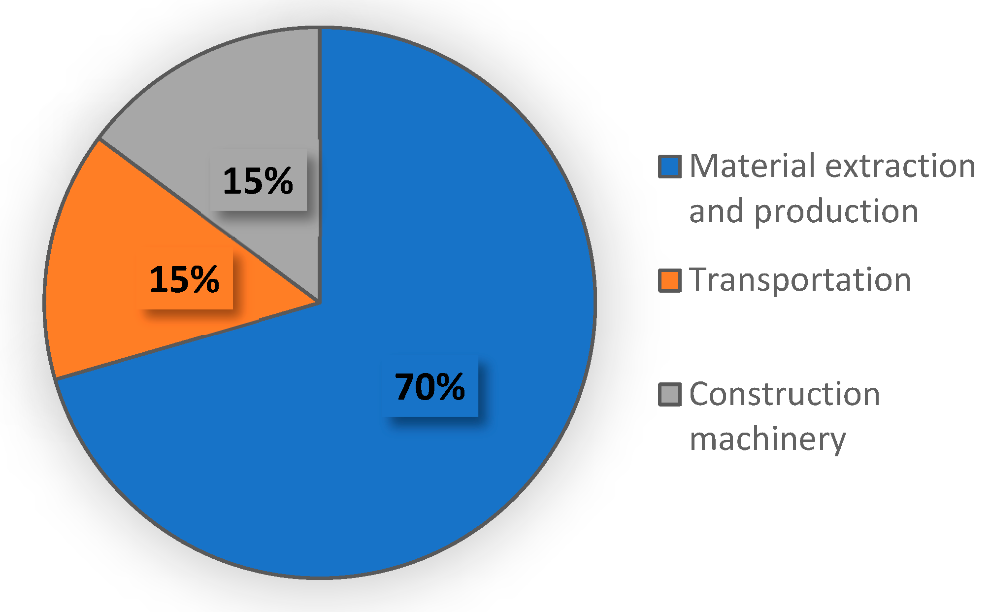
In the case of milling and resurfacing, which were applied in both directions (see Figure 7), the percentage distribution indicates that material extraction and production are the dominant sources of emissions under the baseline scenario analyzed in this study, accounting for 70% of the total. The second-largest source is material transportation, accounting for 15%, while machinery operation contributes the remaining 15%. These results show the relative importance of each component within the modeled intervention scenario and help identify the dominant emission sources associated with this activity.
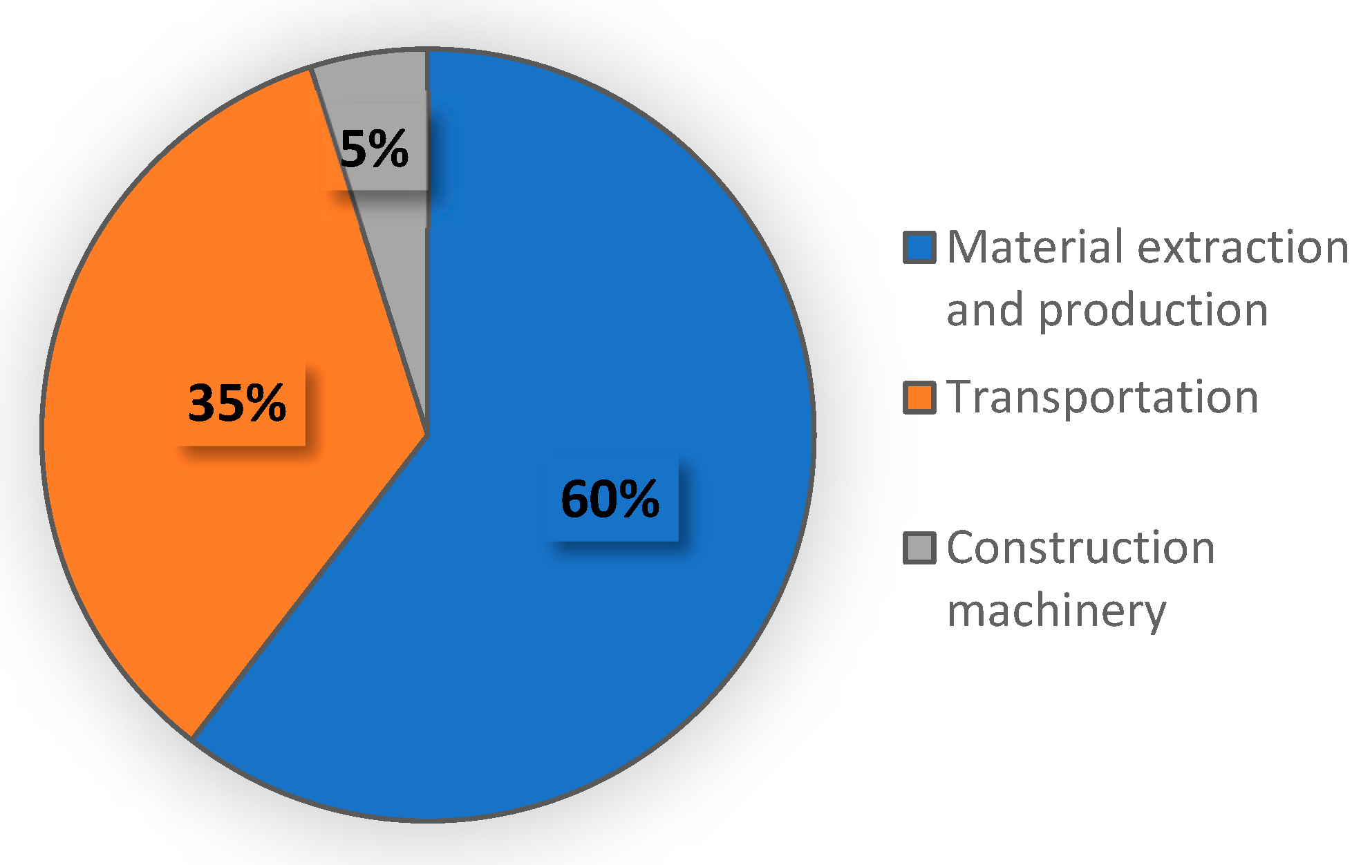
It should be noted that the percentage distributions shown in Figure 7 and Figure 8 correspond to the baseline scenario adopted in this study and should therefore be interpreted as scenario-based estimates. Their relative contribution may vary depending on assumptions related to material and fuel emission factors, transport logistics, equipment fuel-consumption rates, and the quantities of materials associated with each intervention. Consequently, these figures are useful for identifying the dominant emission sources within the analyzed intervention plan, although the exact percentages may change under different local conditions or alternative input assumptions.
The main contributors to CO2e emissions were also identified for each analysis category (see Table 13 and Table 14). HMA production is the most significant component, followed by asphalt binder consumption, while fine and coarse aggregates contribute less. Furthermore, among the emissions attributable to construction equipment used for milling and resurfacing, the pavement milling machine has the greatest environmental impact, followed by the asphalt paver, road roller, and pneumatic tire roller.
For the reconstruction project in the Mexicali–San Felipe direction, Figure 8 shows the percentage distribution of total CO2e emissions. Extraction and production of materials constitute the main source of emissions, with an approximate share of 60%, followed by material transportation (35%) and the use of machinery (5%).
To gain a deeper understanding of the various pavement reconstruction activities, the emissions generated were categorized into three main sources. Table 15 presents the estimated emissions for each structural component of the pavement (subbase, granular base, asphalt base, and asphalt surface course), Table 16 shows the emissions resulting from material hauling distances, and Table 17 shows the emissions generated by the use of construction equipment. Among the reconstruction-related results, material production is dominated by HMA and bituminous binder, transportation emissions are mainly associated with the long-haul movement of granular base and subbase materials, and the motor grader is the largest contributor within the construction machinery category.

5. Discussion

The results of this study facilitate the identification of the processes and activities that predominate in GHG generation during asphalt pavement maintenance under real operating conditions. For the Mexicali–San Felipe section, the largest interventions (milling and overlay and reconstruction) account for the majority of accumulated emissions over the analysis period. These results are directly related to the high volumes of materials required and the energy consumption associated with extraction, production, and on-site placement.
In the specific case of milling and resurfacing, the extraction and production of materials accounts for approximately 70% of total emissions, while transportation and machinery use each contribute around 15%. This distribution reflects the high energy intensity of hot-mix asphalt production and bituminous binders, which are the main inputs for this type of work. Similarly, in the case of reconstruction, although the extraction and production of materials remains the largest contributor (60%), transportation becomes more significant (35%) due to the long material haulage distances (up to 177 km) considered in this case study. This result highlights that, in regions with limited local material availability, such as the desert or semi-arid areas of northwestern Mexico, material transportation can become a critical factor contributing to the environmental impact of pavement.
These results are consistent with previous studies showing that material production and the amount of material used are key drivers of pavement-related emissions [20,30,40]. In the present case, this is reflected in the high contribution of material production to both milling and overlay and reconstruction. The results also confirm that major interventions generate substantially higher emissions than routine maintenance because they require larger volumes of materials and more intensive construction operations. At the same time, the cumulative effect of recurrent low-impact activities such as pothole repair and crack sealing should not be overlooked [26,39,41].
Although previous LCA-based studies have consistently reported that material extraction and production are major contributors to pavement-related emissions [24,58,59,60,61,62,63], the contribution of the present study is not limited to confirming that general trend. Rather, the proposed approach quantifies how emissions are distributed across a 35-year maintenance and rehabilitation plan for a real highway section using HDM-4-based intervention scheduling. The results show that the relative importance of each source varies according to the intervention type: in milling and overlay, material production accounts for about 70% of total emissions, whereas in reconstruction it remains dominant (60%) but is accompanied by a substantial transport contribution (35%) associated with long hauling distances. This provides a more operational perspective for pavement management, since it identifies not only the dominant source of emissions but also the intervention stage and logistics conditions where mitigation actions may be most effective. In addition, machinery-related emissions, although lower than those associated with material production, remain relevant for high-intensity interventions and should not be neglected in simplified environmental assessments of pavement maintenance [64,65,66].
From a road infrastructure management and design perspective, the findings reveal the importance of implementing diverse mitigation strategies to reduce the environmental impact generated by the various activities and processes involved in an intervention plan. Among the most effective alternatives are WMA, on-site material recycling, optimization of transport routes, and the incorporation of more energy-efficient equipment—all of which offer opportunities to reduce emissions. Furthermore, when developing intervention plans for different road projects, these plans should place greater emphasis on preventive maintenance to extend pavement lifespan and reduce the need for major interventions (e.g., reconstruction). This is a key measure for minimizing the environmental impact throughout the pavement’s lifespan.
An important feature of the proposed methodology is that it can be adapted to other road sections where similar information is available, particularly traffic data, pavement condition, material transport distances, and representative emission factors. Its application to other contexts would still require adjustment to local climatic, logistical, and material conditions, but the general framework can support environmental assessment in data-constrained pavement management settings.
Despite its advantages, the proposed methodology has limitations that restrict its scope. Currently, it focuses only on quantifying CO2e emissions associated with material extraction and production, input transportation, and machinery use during pavement maintenance activities. Furthermore, it does not consider other environmental indicators such as acidification, eutrophication, or human toxicity, which, if integrated, would provide a more comprehensive assessment of the environmental impact of road maintenance. Another important limitation is that the emission factors used in the study were taken from international literature sources rather than from Mexico-specific inventories. Although these factors provide a useful reference for estimating the relative contribution of the main emission sources, their absolute values may differ from those that would be obtained using local production data. This is particularly relevant because the energy mix, fuel sources, industrial efficiency, and production technologies used in Mexico may differ from those reported in the literature. Therefore, while the selected factors are appropriate for identifying the dominant processes within the intervention plan, the total CO2e values reported in this study should be interpreted as approximations rather than exact Mexico-specific estimates.
Similarly, this methodology does not account for the environmental impact of the road during the use phase. Emissions generated by vehicles traveling on the roadway, as well as the influence of pavement deterioration and roughness on vehicle fuel consumption over time, were excluded from the present assessment. As a result, the study does not represent the full environmental burden associated with pavement performance over its service life and may underestimate the total impact of the road system. This omission is particularly relevant because changes in pavement condition can affect rolling resistance and vehicle operating efficiency, which in turn may increase user-related emissions during operation. Although these effects are outside the direct boundary of the intervention activities analyzed here, their inclusion would provide a more complete life-cycle perspective and could modify the relative importance of maintenance timing and pavement condition in the overall environmental performance of the roadway.
Another limitation of the study is that the environmental characterization used in HDM-4 was simplified to the closest available climatic category for the study area, without incorporating detailed local variables such as precipitation amount and frequency, wetting-drying cycles, heating-cooling cycles, or traffic intensity under those specific conditions. In addition, no historical local validation of HDM-4 deterioration forecasts against observed pavement deterioration was available for the analyzed section. As a result, the proposed intervention schedule should be interpreted as a model-based planning scenario rather than as a fully locally calibrated prediction of pavement deterioration over time.
In addition, the intervention schedule was configured as a scenario-based representation of routine, periodic, and major rehabilitation actions over the analysis period in order to quantify the emissions associated with the main intervention types considered in pavement management. Therefore, it should not be interpreted as an optimization exercise aimed exclusively at maintaining the lowest possible IRI throughout the full time horizon.
Another limitation of the study is that the intervention plan was generated using a baseline traffic-growth assumption without a formal sensitivity analysis of alternative growth scenarios. Although the adopted rate was estimated from historical AADT records excluding pandemic years, variations in future traffic demand may affect the timing of interventions and the associated CO2e emissions. Future work should evaluate the sensitivity of the maintenance schedule and the emission results to different traffic-growth assumptions.
Another limitation of the study is that the intervention plan was developed at the road-section level and was not spatially disaggregated into specific chainages or localized damage zones. As a result, the analysis does not provide a direct spatial correspondence between the current distribution of pavement deterioration and the exact location of the proposed repair actions. A more detailed spatial allocation of interventions would require pavement-condition data by sub-section or chainage, which were not available for the present case study.
In addition, transport emissions were estimated considering only loaded inbound trips, while return-trip conditions were excluded because they depend on supplier-specific logistics. As a result, the transport component should be interpreted as a simplified estimate.
Likewise, machinery-related emissions were estimated using average fuel-consumption values from technical manuals and published literature rather than project-specific productivity or utilization records. Consequently, the absolute values associated with construction equipment may differ from those that would be obtained from direct field measurements. Future studies should incorporate on-site monitoring, project-specific productivity factors, or sensitivity analyses to improve the accuracy of these estimates.
In this regard, several opportunities for improvement have been identified for future research to strengthen and broaden the scope of the proposed methodology:
  • Incorporate environmental indicators (acidification, eutrophication, or human toxicity) that assess different dimensions of the impact.
  • Develop specific emission factors for materials and construction processes in the road sector in Mexico.

6. Conclusions

This study evaluated the CO2e emissions generated by the intervention plan for an asphalt road connecting the city of Mexicali with San Felipe, Baja California, Mexico. To accomplish this, a simplified LCA-based method was used, combining the HDM-4 pavement management model with emission factors for materials, transportation, and construction equipment. Through this proposed approach, it was possible to identify the activities or processes that contributed most to emissions during the analysis period, under real traffic, weather, and logistics conditions.
Over the 35-year analysis period, the evaluated intervention plan generated approximately 2483.9 t CO2e for the analyzed 7.8 km road section. Reconstruction was the most carbon-intensive activity, accounting for 1890 t CO2e, while milling and overlay generated 292.15 t CO2e per direction. In relative terms, material extraction and production constituted the dominant source of emissions, contributing approximately 70% of total emissions in milling and overlay and 60% in reconstruction, while transportation represented up to 35% of total emissions in the latter case due to long haul distances. These results show that the environmental burden of pavement maintenance is strongly influenced by the scale of intervention, the volume of materials required, and the logistics associated with material supply.
The findings in this study indicate that the size and frequency of pavement maintenance interventions influence the cumulative environmental impact of roads. For example, larger-scale interventions, such as milling, resurfacing, and reconstruction, account for the majority of CO2e emissions due to the large quantities of materials required and the energy needed for their extraction, manufacturing, and installation. On the other hand, routine maintenance tasks generate much lower emissions per unit; however, these types of interventions are applied more frequently over time, resulting in an accumulation that should not be overlooked in road infrastructure planning.
Key Findings:
  • The extraction and production of materials constitute the main source of CO2e emissions in all the interventions analyzed, representing approximately 60% to 70% of total emissions during the analysis period.
  • The transport of materials is of considerable importance in situations where hauling distances are long, representing up to 35% of total emissions in reconstruction projects, especially in regions with limited availability of local materials.
  • The use of construction machinery contributes a smaller fraction compared to the transport of materials and the extraction and production of materials. Equipment such as milling machines, asphalt pavers, and compaction rollers stand out for their long service life and the type of fuel they use.
  • Preventive maintenance interventions, such as crack sealing and pothole repair, generate fewer emissions during their execution and can delay the need for larger-scale rehabilitation work that requires more resources and energy.
  • Integrating pavement management models with environmental assessment methods enables comparisons of conservation options across the life cycle and facilitates decision-making based on environmental criteria.
  • The proposed methodological approach offers a practical and replicable alternative for quantifying CO2e emissions in pavement conservation, aligned with the life cycle approach and designed to support decision-making in road management.
From a practical perspective, this research clearly highlights the importance of incorporating environmental factors into the administration and planning of road maintenance. To achieve this, it is essential to prioritize routine and preventive maintenance, optimize transport distances, adopt construction techniques with lower energy consumption, and reduce the use of virgin materials by incorporating alternative and RAP. These measures offer concrete opportunities to continuously reduce the carbon footprint of asphalt pavements throughout their service life.
Overall, this study highlights the importance of explicitly integrating environmental considerations into road maintenance planning as a pathway toward more sustainable road infrastructure systems. The proposed methodology provides a practical and replicable framework for quantifying greenhouse gas emissions associated with maintenance activities, identifying high-impact processes, and supporting the environmental evaluation of pavement intervention plans based on their emission performance.
When applied at the road-section level and accounting for traffic demand and local conditions, the framework demonstrates its potential to support evidence-based decision-making in both technical management and public policy contexts related to road infrastructure development. Moreover, it provides a robust technical basis for public agencies and road authorities to incorporate environmental criteria into pavement maintenance planning, complementing conventional technical and economic analyses and fostering strategies to progressively reduce emissions and more efficiently use resources.

Author Contributions

Conceptualization, D.F.-R. and M.M.-A.; methodology, D.F.-R. and L.G.; software, D.F.-R. and M.M.-A.; validation, D.F.-R., J.C.-R. and J.M.G.-M.; formal analysis, D.F.-R. and M.M.-A.; investigation, D.F.-R. and L.G.; resources, M.M.-A. and L.G.; data curation, L.G.; writing—original draft preparation, D.F.-R. and M.M.-A.; writing—review and editing, C.S.-B. and A.S.-A.; visualization, J.C.-R. and J.M.G.-M.; supervision, A.S.-A.; project administration, L.G. and J.C.-R. All authors have read and agreed to the published version of the manuscript.

Funding

This research received no external funding.

Institutional Review Board Statement

Not applicable.

Informed Consent Statement

Not applicable.

Data Availability Statement

The original contributions presented in this study are included in the article. Further inquiries can be directed to the corresponding author.

Conflicts of Interest

The authors declare no conflicts of interest.

References

  1. Adu, D.; Du, J.; Asomani, S.N.; Abbey, A. Energy Generation and Carbon Dioxide Emission—The Role of Renewable Energy for Green Development. Energy Rep. 2024, 12, 1420–1430. [Google Scholar] [CrossRef]
  2. Dhakal, S.; Minx, J.C.; Toth, F.L.; Abdel-Aziz, A.; Figueroa Meza, M.J.; Hubacek, K.; Tan, X.C.; Wiedmann, T. Emissions Trends and Drivers. In Climate Change 2022-Mitigation of Climate Change; Shukla, P.R., Skea, J., Slade, R., Al Khourdajie, A., van Diemen, R., McCollum, D., Pathak, M., Some, S., Vyas, P., Fradera, R., et al., Eds.; Cambridge University Press: Cambridge, UK, 2023; pp. 215–294. [Google Scholar]
  3. Strano, E.; Giometto, A.; Shai, S.; Bertuzzo, E.; Mucha, P.J.; Rinaldo, A. The Scaling Structure of the Global Road Network. R. Soc. Open. Sci. 2017, 4, 170590. [Google Scholar] [CrossRef]
  4. Wang, F.; Xie, J.; Wu, S.; Li, J.; Barbieri, D.M.; Zhang, L. Life Cycle Energy Consumption by Roads and Associated Interpretative Analysis of Sustainable Policies. Renew. Sustain. Energy Rev. 2021, 141, 110823. [Google Scholar] [CrossRef]
  5. Laurance, W.F.; Clements, G.R.; Sloan, S.; O’Connell, C.S.; Mueller, N.D.; Goosem, M.; Venter, O.; Edwards, D.P.; Phalan, B.; Balmford, A.; et al. Corrigendum: A Global Strategy for Road Building. Nature 2014, 514, 262. [Google Scholar] [CrossRef]
  6. International Energy Agency (IEA). International Energy Agency (IEA) Statistics: GHG Emissions from Fuel Combustion: Highlights, 2024th ed.; International Energy Agency (IEA): Paris, France, 2024. [Google Scholar]
  7. Wang, J.; Yang, X. Spatial Spillover of Yangtze River Delta Transportation Infrastructure on Economic Growth. Highway 2023, 68, 195–203. [Google Scholar]
  8. Zan, X.; Ou, G. Transport Infrastructure, Internet and Urban Economic Growth Potential. J. Highw. Transp. Res. Dev. 2023, 40, 261–270. [Google Scholar]
  9. Shi, J.; Bai, T.; Zhao, Z.; Tan, H. Driving Economic Growth through Transportation Infrastructure: An In-Depth Spatial Econometric Analysis. Sustainability 2024, 16, 4283. [Google Scholar] [CrossRef]
  10. Chan, H.Y.; Xu, Y.; Wang, Z.; Chen, A. The Deeper and Wider Social Impacts of Transportation Infrastructure: From Travel Experience to Sense of Place and Academic Performance. Transp. Policy 2024, 158, 51–63. [Google Scholar] [CrossRef]
  11. Chan, H.Y.; Xu, Y.; Chen, A.; Zhou, J. Choice and Equity: A Critical Analysis of Multi-Modal Public Transport Services. Transp. Policy 2023, 140, 114–127. [Google Scholar] [CrossRef]
  12. Jiang, X.; He, X.; Zhang, L.; Qin, H.; Shao, F. Multimodal Transportation Infrastructure Investment and Regional Economic Development: A Structural Equation Modeling Empirical Analysis in China from 1986 to 2011. Transp. Policy 2017, 54, 43–52. [Google Scholar] [CrossRef]
  13. Qi, G.; Shi, W.; Lin, K.C.; Yuen, K.F.; Xiao, Y. Spatial Spillover Effects of Logistics Infrastructure on Regional Development: Evidence from China. Transp. Res. Part A Policy Pract. 2020, 135, 96–114. [Google Scholar] [CrossRef]
  14. Song, L.; van Geenhuizen, M. Port Infrastructure Investment and Regional Economic Growth in China: Panel Evidence in Port Regions and Provinces. Transp. Policy 2014, 36, 173–183. [Google Scholar] [CrossRef]
  15. Lu, M.; Luo, Z.; Cang, Y.; Zhang, N.; Yang, L. Methods for Calculating Building-Embodied Carbon Emissions for the Whole Design Process. Fundam. Res. 2025, 5, 2187–2198. [Google Scholar] [CrossRef]
  16. Lai, K.E.; Abdul Rahiman, N.; Othman, N.; Ali, K.N.; Lim, Y.W.; Moayedi, F.; Mat Dzahir, M.A. Quantification Process of Carbon Emissions in the Construction Industry. Energy Build. 2023, 289, 113025. [Google Scholar] [CrossRef]
  17. Labaran, Y.H.; Mathur, V.S.; Muhammad, S.U.; Musa, A.A. Carbon Footprint Management: A Review of Construction Industry. Clean. Eng. Technol. 2022, 9, 100531. [Google Scholar] [CrossRef]
  18. Cheng, S.; Zhou, X.; Zhou, H. Study on Carbon Emission Measurement in Building Materialization Stage. Sustainability 2023, 15, 5717. [Google Scholar] [CrossRef]
  19. Marzouk, M.; El-zayat, M.; Aboushady, A. Assessing Environmental Impact Indicators in Road Construction Projects in Developing Countries. Sustainability 2017, 9, 843. [Google Scholar] [CrossRef]
  20. Zhang, L.; Tian, W.; Wang, B.; Dai, X. Dynamic Life Cycle Assessment of Low-Carbon Transition in Asphalt Pavement Maintenance: A Multi-Scale Case Study Under China’s Dual-Carbon Target. Sustainability 2025, 17, 6540. [Google Scholar] [CrossRef]
  21. Yu, C.; Wu, L.; Liu, Y.; Ye, K.; Liang, G. Estimating Greenhouse Gas Emissions from Road Construction by Considering the Regional Differences in Carbon Emission Factors of Cement: The Case of China. Buildings 2022, 12, 1341. [Google Scholar] [CrossRef]
  22. Frischknecht, R. Lehrbuch der Ökobilanzierung; Springer: Berlin/Heidelberg, Germany, 2020; ISSN ISBN 3662547635. [Google Scholar]
  23. ISO 14040:2006; Environmental Management—Life Cycle Assessment—Principles and Framework. ISO: Geneva, Switzerland, 2006.
  24. Santero, N.J.; Masanet, E.; Horvath, A. Life-Cycle Assessment of Pavements. Part I: Critical Review. Resour. Conserv. Recycl. 2011, 55, 801–809. [Google Scholar] [CrossRef]
  25. Hoxha, E.; Vignisdottir, H.R.; Barbieri, D.M.; Wang, F.; Bohne, R.A.; Kristensen, T.; Passer, A. Life Cycle Assessment of Roads: Exploring Research Trends and Harmonization Challenges. Sci. Total Environ. 2021, 759, 143506. [Google Scholar] [CrossRef] [PubMed]
  26. Du, Y.; Gao, Z.; Liu, C.; Weng, Z.; Ren, X.; Li, W. Comprehensive Review on Greenhouse Gas Emission Assessment over the Full Life-Cycle of Pavement. Case Stud. Constr. Mater. 2025, 22, e04407. [Google Scholar] [CrossRef]
  27. Aryan, Y.; Dikshit, A.K.; Shinde, A.M. Life Cycle Environmental Assessment of State and National Highways in India: Evaluating Impact Reduction Potential of Sustainable Measures. Environ. Impact Assess. Rev. 2025, 114, 107944. [Google Scholar] [CrossRef]
  28. Ataee, S.; Stephan, A. Life Cycle Assessment and Material Flow Analysis of Road and Rail Infrastructure Assets—A Critical Review. Clean. Environ. Syst. 2025, 16, 100259. [Google Scholar] [CrossRef]
  29. Barbhuiya, S.; Das, B.B. Life Cycle Assessment of Construction Materials: Methodologies, Applications and Future Directions for Sustainable Decision-Making. Case Stud. Constr. Mater. 2023, 19, e02326. [Google Scholar] [CrossRef]
  30. Liu, Y.; Liu, Z.; Zhu, Y.; Zhang, H. A Review of Sustainability in Hot Asphalt Production: Greenhouse Gas Emissions and Energy Consumption. Appl. Sci. 2024, 14, 10246. [Google Scholar] [CrossRef]
  31. Oreto, C.; Russo, F.; Veropalumbo, R.; Viscione, N.; Biancardo, S.A.; Dell’acqua, G. Life Cycle Assessment of Sustainable Asphalt Pavement Solutions Involving Recycled Aggregates and Polymers. Materials 2021, 14, 3867. [Google Scholar] [CrossRef]
  32. Martinez-Soto, A.; Calabi-Floody, A.; Valdes-Vidal, G.; Hucke, A.; Martinez-Toledo, C. Life Cycle Assessment of Natural Zeolite-Based Warm Mix Asphalt and Reclaimed Asphalt Pavement. Sustainability 2023, 15, 1003. [Google Scholar] [CrossRef]
  33. Belc, A.L.; Ciutina, A.; Buzatu, R.; Belc, F.; Costescu, C. Environmental Impact Assessment of Different Warm Mix Asphalts. Sustainability 2021, 13, 11869. [Google Scholar] [CrossRef]
  34. Siverio Lima, M.S.; Makoundou, C.; Sangiorgi, C.; Gschösser, F. Life Cycle Assessment of Innovative Asphalt Mixtures Made with Crumb Rubber for Impact-Absorbing Pavements. Sustainability 2022, 14, 14798. [Google Scholar] [CrossRef]
  35. Rodríguez-Alloza, A.M.; Garraín, D. Comparative Life Cycle Assessment of Rubberized Warm-Mix Asphalt Pavements: A Cradle-to-Gate Plus Maintenance Approach. Coatings 2025, 15, 899. [Google Scholar] [CrossRef]
  36. Freire, A.C.; Neves, J.; Plati, C.; Tsakoumaki, M. Life Cycle Assessment (LCA) of Alternative Pavement Rehabilitation Solutions: A Case Study. Sustainability 2023, 15, 2129. [Google Scholar] [CrossRef]
  37. Mantalovas, K.; Graziano, F.; Teresi, R.; Mangano, M.C.; Sarà, G.; Celauro, C. Life Cycle Assessment of Asphalt Mixtures Incorporating Secondary Raw Materials Under a Circular Economy Perspective. Sustainability 2025, 17, 10869. [Google Scholar] [CrossRef]
  38. Flores-Ruiz, D.; Montoya-Alcaraz, M.; García, L.; Gutiérrez, M.; Calderón-Ramírez, J. Mitigation Strategies Based on Life Cycle Assessment for Carbon Dioxide Reduction in Asphalt Pavements: Systematic Review. Sustainability 2025, 17, 695. [Google Scholar] [CrossRef]
  39. Ma, F.; Dong, W.; Fu, Z.; Wang, R.; Huang, Y.; Liu, J. Life Cycle Assessment of Greenhouse Gas Emissions from Asphalt Pavement Maintenance: A Case Study in China. J. Clean. Prod. 2021, 288, 125595. [Google Scholar] [CrossRef]
  40. Wang, Y.; Wang, Y.Q.; Ji, S.J.; Sun, S.J.; Ma, S.H.; Gao, Y.N. Characteristics of Life-Cycle Carbon Dioxide Emissions of Arterial Highway Maintenance and the Influencing Factors. Adv. Clim. Change Res. 2024, 15, 751–765. [Google Scholar] [CrossRef]
  41. Blaauw, S.A.; Maina, J.W.; Mturi, G.A.J.; Visser, A.T. Flexible Pavement Performance and Life Cycle Assessment Incorporating Climate Change Impacts. Transp. Res. D. Transp. Environ. 2022, 104, 103203. [Google Scholar] [CrossRef]
  42. Jain, B.; Tiwari, D.; Parida, M.; Anbanandam, R. Assessment of Vehicular Fuel Consumption and Interaction with Pavement Characteristics Using HDM-4 on Indian Urban Road Network: A Case of Pune City. Case Stud. Constr. Mater. 2022, 17, e01362. [Google Scholar] [CrossRef]
  43. Choi, J. ho Strategy for Reducing Carbon Dioxide Emissions from Maintenance and Rehabilitation of Highway Pavement. J. Clean. Prod. 2019, 209, 88–100. [Google Scholar] [CrossRef]
  44. Jiao, X.; Bienvenu, M. Field Measurement and Calibration of HDM-4 Fuel Consumption Model on Interstate Highway in Florida. Int. J. Transp. Sci. Technol. 2015, 4, 29–45. [Google Scholar] [CrossRef]
  45. Zhu, L.; Li, J.; Xiao, F. Carbon Emission Quantification and Reduction in Pavement Use Phase: A Review. J. Traffic Transp. Eng. 2024, 11, 69–91. [Google Scholar] [CrossRef]
  46. Anthonissen, J.; Van Troyen, D.; Braet, J.; Van Den Bergh, W. Using carbon dioxide emissions as a criterion to award road construction projects: A pilot case in Flanders. J. Clean. Prod. 2015, 102, 96–102. [Google Scholar] [CrossRef]
  47. Aryan, Y.; Dikshit, A.K.; Shinde, A.M. A Critical Review of the Life Cycle Assessment Studies on Road Pavements and Road Infrastructures. J. Environ. Manag. 2023, 336, 117697. [Google Scholar] [CrossRef]
  48. SICT. Datos Viales Estado de México 2018. Secretaria de Comunicaciones y Transporte. 2018. Available online: https://datosviales2020.routedev.mx/login/ (accessed on 22 September 2024).
  49. Odoki, J.B.; Kerali, H.G.R. Analytical Framework and Model Descriptions. In The Highway Development and Management Series; The World Road Association (PIARC): Paris, France, 2000; Volume 4. [Google Scholar]
  50. NOM-012-SCT-2-2017; Sobre el Peso y Dimensiones Máximas con los Que Pueden Circular los Vehículos de Autotransporte Que Transitan En Las Vías Generales de Comunicación de Jurisdicción Federal; Norma Oficial Mexicana México, Diario Oficial de la Federación México, Distrito Federal. Secretaría de Comunicaciones y Transportes (SCT): Ciudad de México, México, 2017.
  51. SICT N·CSV·CAR·1·03·004/21; Determinación Del Índice de Regularidad Internacional (IRI). Secretaría de Infraestructura, Comunicaciones y Transportes (SICT) of Mexico: Ciudad de México, México, 2021.
  52. Ma, H.; Zhang, Z.; Zhao, X.; Wu, S. A Comparative Life Cycle Assessment (LCA) of Warm Mix Asphalt (WMA) and Hot Mix Asphalt (HMA) Pavement: A Case Study in China. Adv. Civ. Eng. 2019, 2019, 9391857. [Google Scholar] [CrossRef]
  53. Stripple, H. Life Cycle Assessment of Road A Pilot Study for Inventory Analysis; IVL Swedish Environmental Research Institute: Gothenburg, Sweden, 2001. [Google Scholar]
  54. Gialos, A.; Zeimpekis, V.; Madas, M.; Papageorgiou, K. Calculation and Assessment of CO2e Emissions in Road Freight Transportation: A Greek Case Study. Sustainability 2022, 14, 10724. [Google Scholar] [CrossRef]
  55. Alaloul, W.S.; Altaf, M.; Musarat, M.A.; Javed, M.F.; Mosavi, A. Systematic Review of Life Cycle Assessment and Life Cycle Cost Analysis for Pavement and a Case Study. Sustainability 2021, 13, 4377. [Google Scholar] [CrossRef]
  56. Bartolozzi, I.; Antunes, I.; Rizzi, F. The Environmental Impact Assessment of Asphalt Rubber: Life Cycle Assessment. In Proceedings of the 5th Asphalt Rubber Conference, Munich, Germany, 23–26 October 2012; pp. 799–819. [Google Scholar]
  57. Eggleston, H.S.; Buendia, L.; Miwa, K.; Ngara, T.; Tanabe, K. 2006 IPCC Guidelines for National Greenhouse Gas Inventories; Institute for Global Environmental Strategies: Kanagawa, Japan, 2006. [Google Scholar]
  58. Wang, X.; Duan, Z.; Wu, L.; Yang, D. Estimation of Carbon Dioxide Emission in Highway Construction: A Case Study in Southwest Region of China. J. Clean. Prod. 2015, 103, 705–714. [Google Scholar] [CrossRef]
  59. Zhou, X.; Zhang, X.; Zhang, Y.; Adhikari, S. Life Cycle Assessment of Asphalt and Cement Pavements: Comparative Cases in Shanxi Province. Constr. Build. Mater. 2022, 315, 125738. [Google Scholar] [CrossRef]
  60. Assaf, H.; Abu Abdo, A. Life Cycle Assessment of Incorporating Recycled Materials in Pavement Design. J. King Saud. Univ. Eng. Sci. 2022, 36, 473–484. [Google Scholar] [CrossRef]
  61. Nauar da Silva, I.; Maués, L.M.F. Inventory of Sand and Pebble Production for Use in Hot Mix Asphalt: A Case Study in Brazil. J. Clean. Prod. 2021, 294, 126271. [Google Scholar] [CrossRef]
  62. Milad, A.; Babalghaith, A.M.; Al-Sabaeei, A.M.; Dulaimi, A.; Ali, A.; Reddy, S.S.; Bilema, M.; Yusoff, N.I.M. A Comparative Review of Hot and Warm Mix Asphalt Technologies from Environmental and Economic Perspectives: Towards a Sustainable Asphalt Pavement. Int. J. Environ. Res. Public Health 2022, 19, 14863. [Google Scholar] [CrossRef]
  63. Giani, M.I.; Dotelli, G.; Brandini, N.; Zampori, L. Comparative Life Cycle Assessment of Asphalt Pavements Using Reclaimed Asphalt, Warm Mix Technology and Cold in-Place Recycling. Resour. Conserv. Recycl. 2015, 104, 224–238. [Google Scholar] [CrossRef]
  64. Liu, N.; Wang, Y.; Bai, Q.; Liu, Y.; Wang, P.S.; Xue, S.; Yu, Q.; Li, Q. Road Life-Cycle Carbon Dioxide Emissions and Emission Reduction Technologies: A Review. J. Traffic Transp. Eng. 2022, 9, 532–555. [Google Scholar] [CrossRef]
  65. Khan, A.U.; Huang, L. Toward Zero Emission Construction: A Comparative Life Cycle Impact Assessment of Diesel, Hybrid, and Electric Excavators. Energies 2023, 16, 6025. [Google Scholar] [CrossRef]
  66. Hasan, U.; Whyte, A.; Al Jassmi, H. Life Cycle Assessment of Roadworks in United Arab Emirates: Recycled Construction Waste, Reclaimed Asphalt Pavement, Warm-Mix Asphalt and Blast Furnace Slag Use against Traditional Approach. J. Clean. Prod. 2020, 257, 120531. [Google Scholar] [CrossRef]
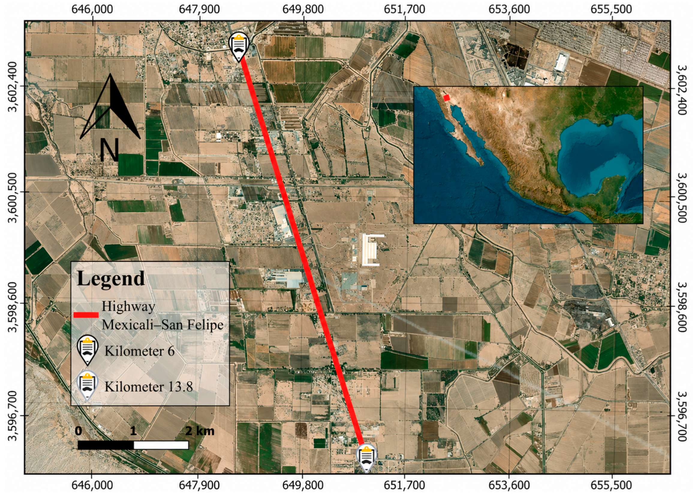
Figure 1. Location of the Mexicali–San Felipe Highway. Source: Prepared by the authors.
Sustainability 18 04461 g001
Figure 2. Methodological framework for quantifying emissions associated with the intervention plan. Source: Authors’ own elaboration.
Sustainability 18 04461 g002
Figure 3. Vehicle classification (VCL) scheme. Source: Authors’ own elaboration with information from SICT [50].
Sustainability 18 04461 g003
Figure 4. Cross-section of the case study. Source: Authors’ own elaboration.
Sustainability 18 04461 g004
Figure 5. Timeline of pavement interventions. Source: Authors’ own elaboration.
Sustainability 18 04461 g005
Figure 6. Modeled IRI evolution for both traffic directions under the adopted intervention scenario during the 2022–2057 analysis period. Source: Authors’ own elaboration.
Sustainability 18 04461 g006
Figure 7. Emission distribution for Milling and Overlay. Source: Authors’ own elaboration.
Sustainability 18 04461 g007
Figure 8. Emission distribution for Reconstruction. Source: Authors’ own elaboration.
Sustainability 18 04461 g008
Table 1. Explicit mapping between the methodological framework and the calculation procedure.
Figure 2 BlockDescriptionOutputEquation
Input dataTraffic, pavement condition, geometry, environmentHDM-4 inputs
HDM-4 analysisGeneration of intervention planActivities and intervention schedule
Inventory compilationMaterials, transport distances, equipment useActivity inventory
Material emissionsAggregates, binder, HMACO2e from material productionEquation (2)
Transport emissionsHauling routes and distancesCO2e from transportationEquation (3)
Machinery emissionsFuel consumption by equipmentCO2e from construction machineryEquation (4)
Total emissionsSum of componentsTotal CO2e per interventionEquation (1)
Source: Authors’ own elaboration.
Table 2. AADT and vehicle fleet composition for the Mexicali–San Felipe highway corridor.
Mexicali–San Felipe
AADT = 13,475
San Felipe–Mexicali
AADT = 11,237
VCLNumber of VehiclesVehicle Share (%)VCLNumber of VehiclesVehicle Share (%)
M8626.4M7536.7
A10,63278.9A892279.4
B2291.7B1911.7
C25664.2C24163.7
C34853.6C34504
T3S24853.6T3S23373
T3S31351T3S31121
T3S2R4810.6T3S2R4560.5
Source: Authors’ own elaboration.
Table 3. Current structural and surface condition of the case study in the year 2022.
CharacteristicMexicali–San FelipeSan Felipe–Mexicali
Surface material typeAsphalt mixtureAsphalt mixture
Surface deflection0.46 mm0.46 mm
International Roughness Index2.48 m/km2.78 m/km
Total cracked area26%8.4%
Mean rut depth12.27 mm12.11 mm
Source: Authors’ own elaboration.
Table 4. Numerical inputs explicitly used in HDM-4 for the intervention-plan analysis.
Input
Category
ParameterValueUnitSource/Note
TrafficBase year2022SICT records
TrafficAADT Mexicali–San Felipe13,475veh/dayTable 2
TrafficAADT San Felipe–Mexicali11,237veh/dayTable 2
TrafficTraffic growth rate (Mexicali–San Felipe)3.6%%/yearCalculated from 2011–2022 historical AADT records, excluding pandemic years
TrafficTraffic growth rate (San Felipe–Mexicali)2.1%%/yearCalculated from 2011–2022 historical AADT records, excluding pandemic years
TrafficVehicle configuration/classificationSee Table 2%Based on SICT standard
Traffic loadingESALsNot entered as an independent inputRepresented through AADT, growth rate, and vehicle configuration in HDM-4
ClimateClimate category in HDM-4Subtropical hot/semi-aridClosest available option for Mexicali conditions
Source: Authors’ own elaboration.
Table 5. Physical condition of the pavement based on the International Roughness Index.
Level of Service (IRI, m/km)
CategoryGoodFairPoor
Intervention project≤2.52.5–3.5>3.5
Source: Authors’ own elaboration.
Table 6. Intervention thresholds used to trigger maintenance and reconstruction activities.
Intervention Thresholds
(IRI, m/km)
Intervention Thresholds (no/km)Intervention Thresholds (%)
NamePeriodic MaintenanceReconstructionPatchingCrack sealing
Adopted intervention thresholds3.54.52510%
Source: Authors’ own elaboration.
Table 7. GHG emissions associated with quarry materials and HMA production.
MaterialGHG Emissions (kg CO2e/t)
Coarse aggregate2.43
Fine aggregate8.69
Bituminous binder173
Hot Mix Asphalt45.5
Source: Authors’ own elaboration with information from [39,52,53].
Table 8. Transport distances for different routes.
Transport RouteDistance (km)
Aggregate supply site—Mixing plant188.56
Mixing plant—Pavement construction site11.72
Aggregate supply site—Pavement construction site177
Source: Authors’ own elaboration.
Table 9. Construction equipment categories considered for fuel-consumption estimation.
Construction Equipment CategoryFuel TypeUnit
Front-end loaderDieselL/h
Pavement milling machineDieselL/h
Asphalt paverDieselL/h
Smooth drum rollerDieselL/h
Pneumatic tire rollerDieselL/h
Motor graderDieselL/h
Vibratory smooth drum rollerDieselL/h
Source: Authors’ own elaboration based on equipment categories and fuel-consumption units reported in previous [55,56].
Table 10. Intervention Plan for the Mexicali–San Felipe direction.
YearType of InterventionWork Quantity (m2)
2024Patching31
2029Crack sealing5720
2030Milling and overlay54,600
2037Crack sealing5720
2040Crack sealing5679
2043Crack sealing5632
2046Crack sealing5579
2049Crack sealing5520
2052Crack sealing5856
2055Crack sealing6030
2057Reconstruction54,600
Source: Authors’ own elaboration.
Table 11. Intervention Plan for the San Felipe–Mexicali direction.
YearType of InterventionWork Quantity (m2)
2024Patching30
2025Patching43
2026Patching32
2027Milling and overlay54,600
2037Crack sealing5846
2040Crack sealing5826
2043Crack sealing5804
2046Crack sealing5779
2049Crack sealing5752
2052Crack sealing5722
2055Crack sealing5688
2057Crack sealing6030
Source: Authors’ own elaboration.
Table 12. Emissions by each type of intervention and normalized emissions for the analyzed section.
DirectionInterventionEmissions
(t CO2e)
Normalized Emissions
(t CO2e/km)
Mex-SFPatching0.0240.003
Crack sealing4.400.564
Milling and overlay292.1537.46
Reconstruction1890.00242.31
SF-MexPatching0.080.010
Crack sealing5.100.654
Milling and overlay292.1537.46
Source: Authors’ own elaboration.
Table 13. Emission distribution from material extraction and production (Milling and Overlay).
InputEmissions
(t CO2e)
HMA Production285.75
Coarse aggregate13.98
Fine aggregate30.99
Bituminous binder81.21
Source: Authors’ own elaboration.
Table 14. Emission distribution from machinery use (Milling and Overlay).
Type of MachineryEmissions
(t CO2e)
Pavement milling machine58.27
Asphalt paver9.47
Smooth drum roller8.44
Pneumatic tire roller8.44
Front-end loader1.91
Source: Authors’ own elaboration.
Table 15. Emission distribution from material extraction and production (Reconstruction).
Pavement LayerMaterialsEmissions
(t CO2e)
SubbaseCoarse aggregate30.54
Fine aggregate101.5
Granular baseCoarse aggregate51.75
Fine aggregate114.67
Asphalt baseCoarse aggregate22.73
Fine aggregate40.67
Bituminous binder146.73
HMA428.63
Asphalt surface layerCoarse aggregate6.99
Fine aggregate15.49
Bituminous binder40.6
HMA142.9
Source: Authors’ own elaboration.
Table 16. Emission distribution from material transportation (Reconstruction).
Pavement LayerRouteDistance
(km)
Emissions
(t CO2e)
SubbaseQuarry—Mixing Plant177200
Granular baseQuarry—Mixing Plant177282.48
Asphalt baseQuarry—Mixing Plant188.56122
Mixing Plant—Construction Site11.726.77
Asphalt surface layerQuarry—Mixing Plant188.5640.67
Mixing Plant—Construction Site11.722.26
Source: Authors’ own elaboration.
Table 17. Emission distribution from machinery use (Reconstruction).
Type of MachineryEmissions
(t CO2e)
Contribution
Asphalt paver10.6411.5%
Smooth drum roller23.5425.4%
Pneumatic tire roller14.6815.8%
Front-end loader12.113%
Motor grader31.8234.3%
Source: Authors’ own elaboration.
Disclaimer/Publisher’s Note: The statements, opinions and data contained in all publications are solely those of the individual author(s) and contributor(s) and not of MDPI and/or the editor(s). MDPI and/or the editor(s) disclaim responsibility for any injury to people or property resulting from any ideas, methods, instructions or products referred to in the content.