Global Patterns of Ecosystem Transpiration and Carbon–Water Coupling: An Intercomparison of Four Partitioning Models Using Eddy Covariance Data for Sustainable Water Management

Abstract

Ecosystem transpiration (T) is the core process in terrestrial water and carbon cycles. Accurately estimating T is critical to improving evapotranspiration (ET) models and understanding global ecosystem responses to climate change. In this study, we evaluated four ET partitioning methods (TEA, Z16, L19, and Y21) using 368 global eddy covariance (EC) sites and 15 sap flow sites. Intercomparison results showed that TEA, Z16, and Y21 maintained good consistency, whereas L19 exhibited lower agreement, primarily due to its high sensitivity to energy closure errors and poor non-linear fitting accuracy under extreme conditions. Validation against sap flow data indicated that Z16 performed best (R² = 0.45, KGE = 0.52), followed by Y21, while TEA had the lowest accuracy due to systematic overestimation driven by unremoved persistent background soil evaporation in its training dataset. Global analysis revealed that mean annual T ranged from 213 mm yr⁻¹ (Z16) to 294 mm yr⁻¹ (TEA), with annual T/ET varying between 0.45 (Z16) and 0.63 (TEA). Trend analysis further showed consistent increasing trends across all four methods for both annual T (0.33–0.83 mm·yr⁻²) and annual T/ET (0.0015–0.0019 yr⁻¹). Additionally, a notably stronger relationship was found between gross primary productivity (GPP) and T than between GPP and ET. Despite substantial differences in model structures, these methods effectively capture the temporal dynamics of T and the coupled relationships between ecosystem carbon and water fluxes. Our findings provide critical benchmarks for terrestrial water cycle modeling and sustainable water resource management under a changing climate.

1. Introduction

Evapotranspiration (ET), the amount of water evaporated from the land surface into the atmosphere, is the largest efflux of the terrestrial water cycle, which encompasses two components: biological vegetation transpiration (T) and physical soil (and canopy interception) evaporation (E) [1]. Among them, T predominates in terrestrial ET, contributing 60–90% [2]. To date, numerous studies have achieved reasonably consistent estimates of ET [3,4,5,6]. However, considerable disparities persist across different ET estimation models in partitioning ET into T and E [7,8,9]. Moreover, these individual components exhibit divergent responses to climate change [10,11]. Therefore, accurately partitioning ET into T and E is pivotal for obtaining a holistic understanding of the terrestrial water cycle. Furthermore, it improves the parameterization and calibration of ET estimation models, providing deeper insights into ecosystem feedback on climate change.

Direct measurement of T at the field or ecosystem scale is expensive and difficult, but is becoming more common with the availability of water vapor isotope analyzers and sap flow sensors [12,13]. Based on the principle of isotopic mass balance and the distinct kinetic fractionation effects for T and E, which are two independent processes, stable isotopic techniques can effectively partition ET by analyzing the differences in their isotopic compositions [1]. The application of the stable isotope methods is growing [14,15]; nevertheless, the techniques are limited by their high cost and multiple model assumptions and are unable to obtain long-term continuous measurements [16]. Moreover, T or the ratio of T to ET (T/ET) obtained by stable isotopic methods are usually not easily comparable with those of other non-isotopic methods [13]. Sap flow methods, designed to measure the flow of sap within a plant stem or trunk, are currently the dominant method to estimate tree-scale T measurements and directly assess T products [8]. The sap flow technique provides a quite cost-effective solution for long-term measurement of plants’ transpiration, but obtaining reliable measurements depends on accurate probe placement, calibration, and consideration of wood thermal properties [17]. Sap flow data generally contains noise, outliers, and gaps due to environmental factors, sensor failures, or data collection interruptions. Therefore, data processing, cleaning, and gap-filling are essential for accurate analysis. Recently, the first global compilation of whole-plant transpiration data from sap flow measurements (SAPFLUXNET) has been established [18]. It is a coordinated network of quality-controlled sap-flow datasets and has broad bioclimatic coverage. Overall, the release of SAPFLUXNET facilitates direct T validation and promotes research on ET partitioning [8,19]. However, sap flow measurements are typically conducted on dominant trees within a stand or ecosystem, which ignores the small or non-representative tree species and subcanopy vegetation. Consequently, uncertainties remain when upscaling tree-level measurements to the ecosystem level [20], yet sap flow serves as a critical independent benchmark for validating T estimates.

At the ecosystem scale, the eddy covariance (EC) technique serves as a standard method for directly measuring the exchanges of water and carbon fluxes between the land surface and the atmosphere [21], and it has been widely used over the globe and has led to the establishment of multiple regional flux networks and a global collaborative network (i.e., FLUXNET) [22]. However, a fundamental limitation of the EC method is that it observes the net ecosystem fluxes (e.g., net ecosystem exchange (NEE), ET). Specifically, EC observations do not partition ecosystem carbon fluxes into gross primary productivity (GPP) and ecosystem respiration, nor do they disentangle ET into T and E [23,24]. This inability to quantify the key intermediate fluxes, particularly T, poses a significant challenge to investigating the interactions between the ecosystem water cycle and climate change.

Various methods have been developed to partition ET based on EC data, aiming to obtain long-term continuous T data and calibrate ET estimation models. Those methods have attracted widespread interest in recent years due to their advantages in temporal continuity, spatial representativeness, and time- and labor-efficiency [16]. For example, Scanlon and Sahu [25] developed an ET partitioning method based on flux variance similarity and the original high-frequency measurement of EC data. This method is conceptually simple and the data requirements are modest, while a key parameter, i.e., water use efficiency (WUE), requires leaf-level measurements or intercellular CO₂ concentration data for estimation [21,26]. Based on the WUE concept, Zhou et al. [27], Nelson et al. [28], and Yu et al. [16], respectively, proposed three ET partitioning methods: one based on the underlying WUE index, another utilizing a random forest model for GPP/T estimation, and the third integrating the unified stomatal conductance model for T estimation. All three methods are straightforward in principle and require fewer input variables. However, the methods developed by Zhou et al. [27] and Nelson et al. [28] are predicated on the assumption that T≈ET holds for portions of the growing season [29,30]. According to the inverted Penman–Monteith equation and the stomatal conductance model developed by Medlyn et al. [31], Li et al. [32] and Hu and Lei [33] achieved T/ET estimation at the daily scale via the calculation of canopy conductance. In contrast, the two methods are relatively more complex and involve more input variables. Additionally, many data-driven algorithms (like artificial neural networks) have been applied for ET partitioning at some EC sites, based on the assumption that nighttime T is close to zero to train the model and predict daytime E [23,34]. Compared to other ET partitioning methods, the data-driven ET partitioning methods have few assumptions and good applicability even in spatially heterogeneous sites with large E contributions (e.g., the wetland EC sites). Various ET partitioning methods exist, including methods which are not mentioned here [35,36,37], yet each is subject to multi-faceted limitations. These inherent constraints can introduce systematic biases into the estimated T and T/ET, leading to considerable discrepancies across different approaches. In a comparative analysis of three ET partitioning methods across 251 FLUXNET sites globally, Nelson et al. [38] reported that the estimated T/ET varied from 0.45 to 0.77. Scott et al. [29] compared the seasonal and interannual variability of T/ET from four ET partitioning methods across two EC sites. While all methods showed good agreement in their temporal patterns, substantial differences were observed in the magnitude of monthly and annual T/ET. Therefore, there is no universally recognized, highly accurate method for ET partitioning, and a systematic and comprehensive assessment of those ET partitioning methods for T estimation accuracy and consistency is still lacking. Specifically, existing comparative studies often suffer from two major research gaps: first, a lack of large-scale global validation using independent benchmark datasets, such as sap flow measurements; second, an insufficient analysis of the interannual carbon–water coupling relationships across diverse ecosystem types. Addressing these gaps is not only fundamentally important for improving terrestrial ecohydrological models, but also serves as a critical scientific basis for sustainable agricultural practices and water resource management.

The primary aim of this study is to evaluate the performance of four different ET partitioning methods for T and T/ET estimation across 368 EC sites globally to support sustainable water and agricultural management. Specifically, the objectives are to: (1) evaluate the consistency and accuracy of different ET partitioning methods on T estimates at daily and annual time scales, aided by validation against sap flow measurements from SAPFLUXNET; (2) analyze the spatiotemporal patterns of T/ET and T derived from the four methods, in order to illustrate their consistency in interannual variability; (3) examine the correlation between T (and ET) and GPP to elucidate the coupling relationship between ecosystem carbon and water cycles, and to further assess the reliability of the T estimates. Our results could provide critical insights for ET partitioning by elucidating the strengths and limitations of the four methods, improve our understanding of the ecosystem carbon–water coupling relationship, and facilitate the validation and optimization of ET estimation models under the framework of global water sustainability.

2. Materials and Methods

2.1. Data

2.1.1. Eddy Covariance Measurements

The EC measurements used in this study were downloaded from the FLUXNET2015 dataset [22], the Integrated Carbon Observation System (ICOS 2020 Warm Winter Ecosystem Eddy Covariance Flux Product) [39], and the AmeriFlux network [40]. Based on EC measurements, ecosystem carbon and water fluxes (e.g., ET) and various meteorological variables for different ecosystem types were originally observed at high frequencies (typically 10 Hz or 20 Hz). After standard processing [22], they were aggregated to half-hourly to yearly resolution. In this study, half-hourly observations were used, with the variables including timestamp, air temperature (TA_F), vapor pressure deficit (VPD_F), atmospheric pressure (PA_F), gross primary productivity (GPP_NT_VUT_REF), CO₂ mole fraction (CO2_F_MDS), latent heat flux (LE_F_MDS), sensible heat flux (H_F_MDS), soil heat flux (G_F_MDS), net radiation (NETRAD), friction velocity (USTAR), incoming shortwave radiation (SW_IN), relative humidity (RH), and wind speed (WS).

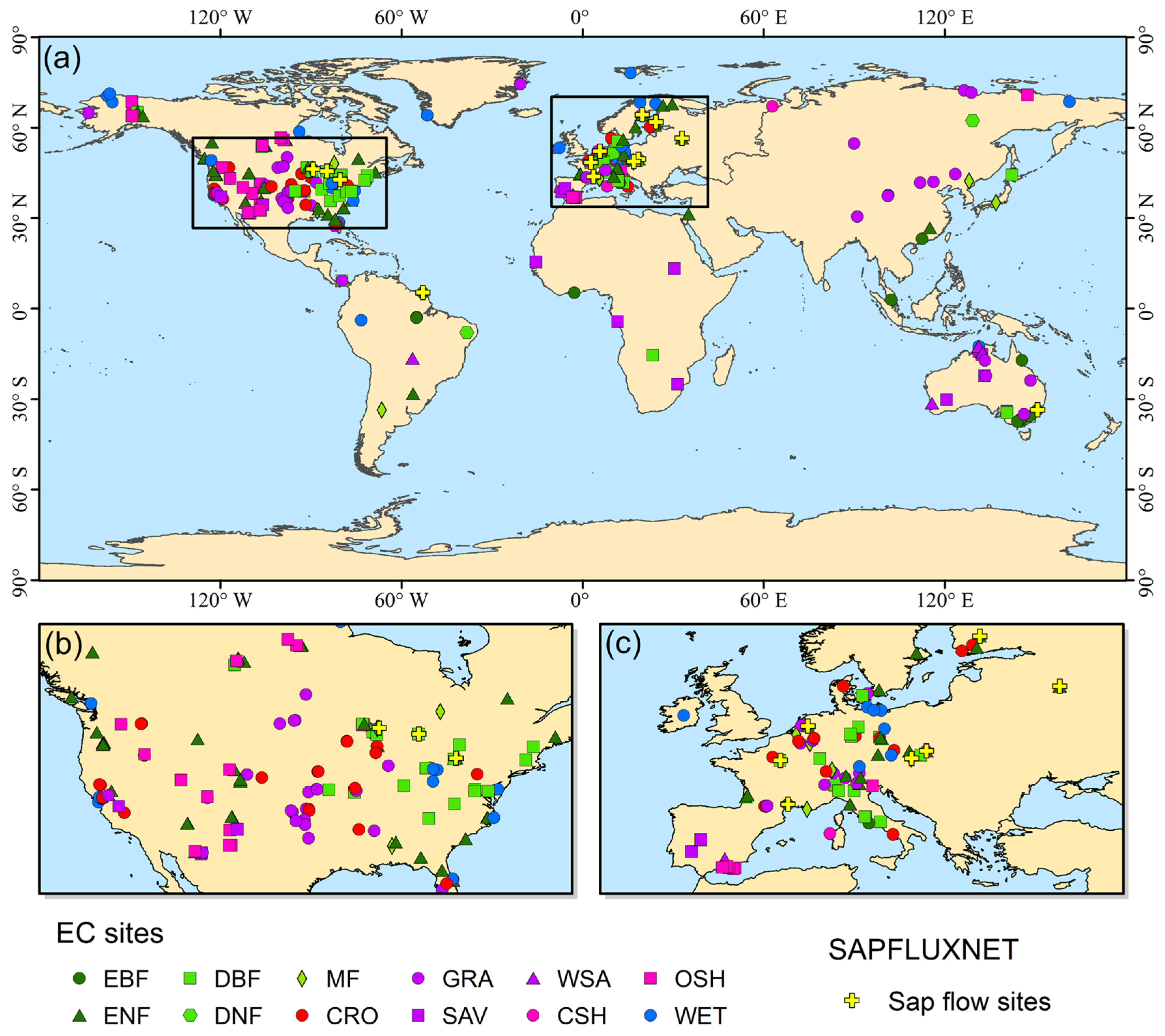
To ensure a consistent and robust comparison among the four ET partitioning methods, a unified data filtering and quality control procedure was applied to the half-hourly flux data. First, only daytime data were selected, which were identified by the NIGHT variable being equal to 0. Second, to guarantee data reliability, only high-confidence data were retained by strictly filtering the quality control (QC) flags; specifically, only originally measured data (QC = 0) or the most reliable gap-filled data (QC = 1) were used. Third, anomalous records, including negative values for gross primary productivity, latent heat flux, and vapor pressure deficit, were excluded. For temporal aggregation, daily values were calculated only when at least 10 valid half-hourly observations were available within a given day. Furthermore, annual aggregations required a minimum of 80% valid days within a year to be included in the interannual analysis. Other method-specific processing details strictly followed their respective original studies [27,28,32]. Following these rigorous quality control procedures, 368 sites were finally selected for analysis (Figure 1).Additionally, based on the International Geosphere–Biosphere Programme (IGBP) classification system, the 368 sites were divided into 12 ecosystem types: evergreen needleleaf forests (ENF, 79 sites), evergreen broadleaf forests (EBF, 15 sites), deciduous broadleaf forests (DBF, 45 sites), deciduous needleleaf forests (DNF, 2 sites), mixed forests (MF, 13 sites), croplands or cropland/natural vegetation mosaics (CRO, 49 sites), grasslands (GRA, 64 sites), savannas (SAV, 15 sites), woody savannas (WSA, 10 sites), open shrublands (OSH, 29 sites), closed shrublands (CSH, 7 sites), and permanent wetlands (WET, 40 sites). The inclusion of these globally distributed ecosystems ensures that our evaluation provides robust benchmarks for sustainable water management across different environmental constraints.

2.1.2. Soil Moisture Data

Soil moisture data in this study served as a pivotal variable for fitting ecosystem conductance. Due to the lack of soil moisture observations at many sites and the existence of substantial gaps in observations, we utilized soil moisture data from the ERA5-Land climate reanalysis dataset produced by the European Centre for Medium-Range Weather Forecasts (ECMWF) [41]. This dataset provides hourly volumetric soil water content at 0.1° spatial resolution. Here those data were obtained from the Google Earth Engine platform [42] according to the spatial locations of EC sites. Although the dataset provides multiple depth layers, the 0–7 cm layer (i.e., volumetric_soil_water_layer_1) was used, and to align with the temporal coverage of the EC observations, hourly soil moisture data were linearly interpolated to half-hour (30 min) intervals.

2.1.3. Sap Flow Data

Sap flow measurements from SAPFLUXNET v0.1.5 were used as the primary data for directly evaluating the accuracy of ET partitioning methods (i.e., T estimation) [18]. In this dataset, plant-level sap flow at sub-daily resolution was quality controlled and corrected. To obtain daily T at the stand level, plant-level sap flow data (cm³ h⁻¹) were first normalized by basal area to derive sap flow per unit basal area (cm³ cm⁻² h⁻¹), and then averaged for each species at each site (i.e., species-level sap flow per unit basal area, cm³ cm⁻² h⁻¹). Secondly, species-specific total sap flow (cm³ h⁻¹) was calculated as the product of the species-level sap flow per unit basal area and the total basal area occupied by that species within the stand. Thirdly, the species-specific total sap flow of all species in the stand was summed to obtain the total sap flow at the stand level (cm³ h⁻¹). If there were any species not measured in the stand, the stand-level total sap flow was rescaled to account for the basal area of unmeasured species [19]. Finally, daily T (cm³ d⁻¹) in this study was summed across all hours of the daytime, which was distinguished using the NIGHT variable of the EC data. After data preprocessing and site filtering to match EC sites, 15 sap flow sites were retained for validating the accuracy of ET partitioning (Figure 1 and

Table 1. Details of the 15 SAPFLUXNET sites used for validating ET partitioning methods in this study. Abbreviations: St Basal Area = total stand basal area (m² ha⁻¹); St Density = total stem density for stand (stems ha⁻¹).

Site ID	Latitude (°)	Longitude (°)	Ecosystem	St Basal Area	St Density	Years
AU-Cum	−33.62	150.74	EBF	27.6	800	2012–2014
FR-Pue	43.74	3.6	EBF	28.1	7149	2000–2015
GF-Guy	5.28	−52.92	EBF	30.6	550	2014–2016
FR-Fon	48.48	2.78	DBF	25	1104	2006–2014
US-UMB	45.56	−84.71	DBF	25	750	2010–2016
US-Umd	45.56	−84.7	DBF	19.1	600	2010–2016
CZ-Lnz	48.68	16.95	MF	30.3	240	2016
US-Syv	46.24	−89.35	MF	33.1	n.a.	2014–2016
CA-TP3	42.71	−80.35	ENF	40	1583	2008–2016
CA-TP4	42.71	−80.36	ENF	36	321	2008–2016
CZ-BK1	49.49	18.53	ENF	36.96	1228	2015–2016
FI-Hyy	61.85	24.29	ENF	20	684	2013–2016
NL-Loo	52.17	5.74	ENF	24.4	434	2012–2015
RU-Fyo	56.46	32.92	ENF	31.6	678	1999–2004
SE-Svb	64.26	19.77	ENF	38.5	869	2016–2017

).

2.2. ET Partitioning Methods

2.2.1. TEA Method

The Transpiration Estimation Algorithm (TEA), developed by [28], utilizes a random forest regressor to train WUE (GPP/ET (T ≈ ET)) and estimate T (hereafter T_TEA) as the GPP (μmol m⁻² s⁻¹) to WUE ratio. The main procedure involves two steps: (1) identifying the time periods when T is closest to ET, i.e., T/ET ≈ 1. Here the time periods are identified using the conservative surface wetness index (CSWI). (2) The random forest model is trained to capture the temporal dynamics of WUE during the identified time periods, and then estimates WUE at every time step. T_TEA is finally obtained as

$$T_{TEA}={\displaystyle \frac{GPP}{WU{E}_{t,pred}}}$$

(1)

$$WU{E}_{t,pred}=R{F}_{75th}(R_g,T_a,RH,u,\dots \dots )$$

(2)

where WUE_t,pred is the predicted WUE value according to the trained random forest regression, and 75th is the 75th percentile recommended by [28]. Rg (incoming radiation, W m⁻²), T_a (air temperature, °C), RH (relative humidity, %), and u (wind speed, m s⁻¹) are the input climatic variables of the random forest model.

The TEA approach is attractive because it relies minimally on physiological assumptions and has high temporal resolution. However, it requires some sufficient dry-surface periods where E is minimized and ET is mostly dominated by T for training the RF model, and if E remains persistent, T may be overestimated unless the quantile selection is carefully tuned.

2.2.2. Z16 Method

The Z16 method [27] is based on the concept of uWUE which is defined at the ecosystem scale as:

$$uWUE={\displaystyle \frac{GPP\sqrt{VPD}}{ET}}$$

(3)

The Z16 method defines a potential uWUE (uWUE_p) that is associated with T, and an apparent uWUE (uWUE_a) that is related to ET. Subsequently, T/ET is estimated as:

$${\displaystyle \frac{T}{ET}}={\displaystyle \frac{uWU{E}_a}{uWU{E}_p}}$$

(4)

$$uWU{E}_a={\displaystyle \frac{GPP\times \sqrt{VPD}}{ET}}$$

(5)

$$uWU{E}_p={\displaystyle \frac{GPP\times \sqrt{VPD}}{T}}$$

(6)

uWUE_p is considered a constant for each site when the ecosystem is homogenous and under steady state conditions, and its value is close to the maximum of uWUE_a when soil evaporation is negligible [30]. In this study, uWUE_p is derived from the 95th-percentile regression between $GPP\times \sqrt{VPD}$ and ET, representing the conditions where T ≈ ET. uWUE_a is directly estimated from half-hourly GPP, VPD (hPa) and ET data at the daily scale. The Z16 method is computationally simple with fewer variables used, and thus it has been widely used at EC sites. However, this method may overestimate T under permanently wet conditions or when soil evaporation cannot be ignored.

2.2.3. L19 Method

The L19 method [32] for ET partitioning is based on the inverted Penman–Monteith (PM) equation and an ecosystem conductance model which generalized Leuning’s model and Medlyn’s model [31,32,43]. By integrating the inverted PM equation and the ecosystem conductance model, the L19 method can partition the ecosystem conductance (G_s) inferred from the PM equation into the canopy conductance (G_veg) and soil conductance, and T/ET is thus estimated as:

$${\displaystyle \frac{T}{ET}}={\displaystyle \frac{G_{veg}}{G_s}}$$

(7)

$$G_s={\displaystyle \frac{\gamma G_{a}LE}{\mathsf{\Delta }(R_n-G)+\rho c_p{G}_{a}VP{D}_a-(\mathsf{\Delta }+\gamma )LE}}$$

(8)

$$G_s=G_0+G_1{\displaystyle \frac{GPP}{VP{D}_l^m}}$$

(9)

$$G_{veg}=G_1{\displaystyle \frac{GPP}{VP{D}_l^m}}$$

(10)

For Equation (8), G_s is calculated according to the inverted PM equation, while for Equation (9), G_s is expressed as the sum of G_veg and soil conductance. Detailed explanation of the parameters in the inverted PM equation (Equation (8)) and the ecosystem conductance model (Equation (9)) can be found in [32,43].

There are three unknown parameters (i.e., G₀, G₁, m) for estimating T/ET. In this study, we used the non-linear least squares (NLLS) regression model to fit the three parameters in each soil moisture category, including the 0–15th, 15–30th, 30–50th, 50–70th, 70–85th, and 85–100th percentiles. During the specific fitting process, the non-linear ecosystem conductance model (Equation (9)) was evaluated to minimize the residual sum of squares between the inverted and modeled Gs. The parameter setting basis relied on ensuring physiological realism; thus, the three parameters were constrained to strict physical bounds, with G₀ ranging from 0 to 5, G₁ from 0 to 50, and m from 0.1 to 5. Furthermore, to guarantee statistical robustness and avoid overfitting, the NLLS regression was only executed when a minimum of 30 valid half-hourly observations were available within a given soil moisture bin.

Specifically, to ensure data continuity for soil moisture binning, soil moisture data from the ERA5-Land reanalysis dataset were exclusively utilized across all sites rather than the actual measurements at the EC sites, which are frequently missing or measured at inconsistent depths. Other data filtering steps followed [32]. This method is physically complex, but avoids the assumption T ≈ ET in the TEA and Z16 methods. Additionally, compared to them, the L19 method requires more input variables, especially for soil moisture data, as its observation is relatively scarce at EC sites.

2.2.4. Y21 Method

The Y21 method [16] is also proposed based on the carbon and water coupling relationship (i.e., WUE). This method uses two WUE concepts, ecosystem WUE (WUE_eco, Equation (11)) and ecosystem transpiration WUE (iWUE_eco, Equation (12)).

$$WU{E}_{eco}={\displaystyle \frac{GPP}{ET}}$$

(11)

$$iWU{E}_{eco}={\displaystyle \frac{GPP}{T}}$$

(12)

T/ET is thus calculated by the ratio of WUE_eco and iWUE_eco:

$${\displaystyle \frac{T}{ET}}={\displaystyle \frac{WU{E}_{eco}}{iWU{E}_{eco}}}$$

(13)

Under steady state environmental conditions, T can be described following Fick’s law [44]:

$$T=1.6g_s{\displaystyle \frac{(e_i-e_a)}{P_a}}=1.6g_s{\displaystyle \frac{VPD}{P_a}}$$

(14)

Here, g_s is the stomatal conductance (mol m⁻² s⁻¹), while (e_i − e_a) is the water vapor pressure difference between the leaf interior and the ambient air and is approximated by VPD. P_a is the atmospheric pressure (hPa). According to the stomatal conductance model developed by [31], g_s is calculated as

$$g_s=\left(1+{\displaystyle \frac{g_1}{\sqrt{VPD}}}\right){\displaystyle \frac{GPP}{C_a}}$$

(15)

where C_a is the ambient atmospheric CO₂ concentration (μmol CO₂ mol⁻¹). Combining Equations (12), (14) and (15), iWUE_eco is expressed as follows:

$$iWU{E}_{eco}={\displaystyle \frac{GPP}{T}}={\displaystyle \frac{C_a{P}_a}{1.6(VPD+g_1\sqrt{VPD})}}$$

(16)

Substituting these equations yields:

$${\displaystyle \frac{T}{ET}}={\displaystyle \frac{WU{E}_{eco}}{iWU{E}_{eco}}}={\displaystyle \frac{\frac{GPP}{ET}}{\frac{C_a{P}_a}{1.6(VPD+g_1\sqrt{VPD})}}}$$

(17)

The Y21 method requires five input variables (GPP, ET, VPD, C_a, P_a, and g₁). Among them, except for g₁, other variables can be directly obtained from half-hourly EC data. It should be explicitly noted that 0% of the sites required the use of globally averaged C_a values or meteorological values derived from ERA5 for this method. Instead, 100% of the C_a input was strictly sourced from the in situ FLUXNET observations, and time steps with missing in situ C_a were excluded to prevent the introduction of external uncertainties. To estimate the parameter g₁, rather than using the site-specific g₁ value from a global g₁ map recommended by [16], we adopted an OLS regression model to fit the g₁ value based on Medlyn’s model [45] for each year at each site. The specific fitting process was based on the standard Medlyn model (Equation (18)), which is expressed as follows:

$$G_s=g_0+1.6\cdot \left(1+{\displaystyle \frac{g_1}{\sqrt{VPD}}}\right)\cdot {\displaystyle \frac{GPP}{C_a}}$$

(18)

Following the recommendations for ecosystem-scale applications [31,45], the parameter setting basis involved forcing the minimum stomatal conductance (g₀) to zero. This assumption is crucial because simultaneously fitting g₀ and g₁ at the canopy scale often leads to severe multicollinearity, which hampers the robustness of the g₁ estimation. By setting g₀ = 0, the model was mathematically transformed into a linear relationship, and g₁ was straightforwardly determined as the slope of the OLS regression through the origin.

2.2.5. Evaluation Metrics

In this study, four metrics—coefficient of determination (R²), root mean square error (RMSE), Kling–Gupta efficiency (KGE), and bias—were used to evaluate the performance of the four ET partitioning methods. KGE is a comprehensive metric ranging from −$\infty$ to 1, as defined in Equation (19), which not only reflects the accuracy of model prediction, but also measures the model’s ability to reproduce the variability and temporal dynamics of observed data [46]. Its calculation integrates the correlation (r), variability (α), and bias (β). Under the ideal condition with no estimation errors, the corresponding value of KGE is 1 [47].

$$KGE=1-\sqrt{{(r-1)}^2+{(\alpha -1)}^2+{(\beta -1)}^2}$$

(19)

where r is the Pearson correlation coefficient, α is the ratio of the standard deviation of simulations to that of observations, and β is the ratio of the mean of simulations to the mean of observations.

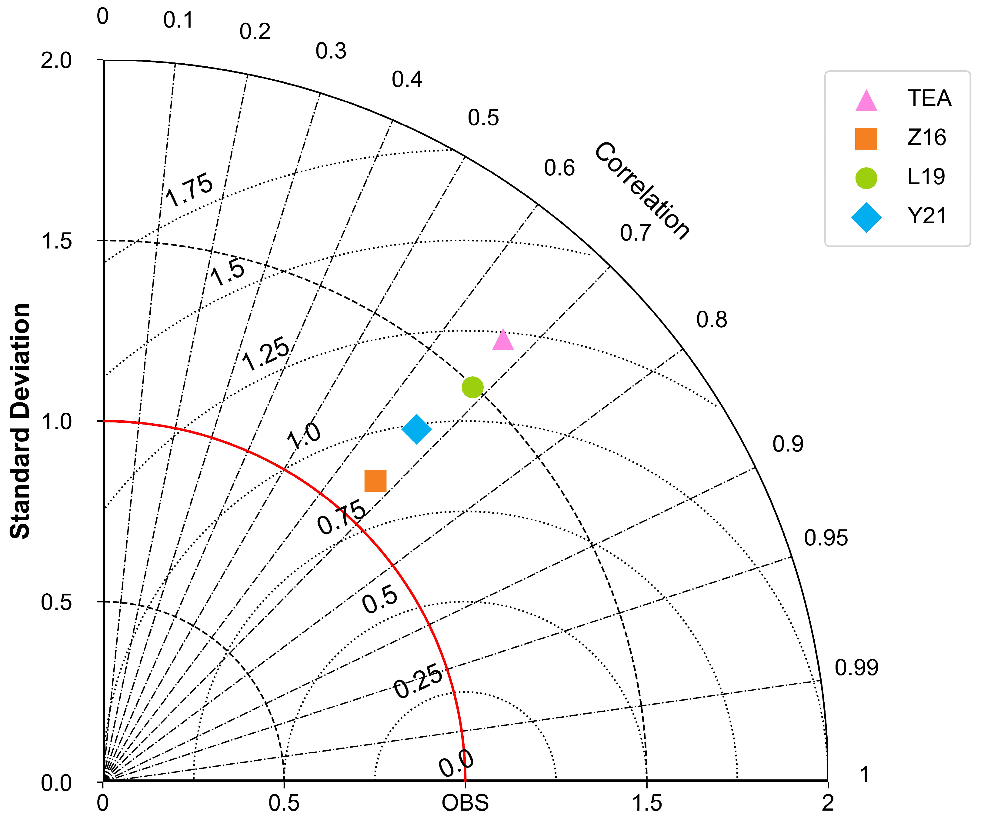
Furthermore, to provide a comprehensive multidimensional evaluation, a normalized Taylor diagram [48] was utilized. This diagram visually integrates the correlation coefficient (R), the normalized standard deviation (SD), and the centered root mean square error (CRMSE), allowing for a simultaneous comparison of the temporal consistencies and amplitude accuracies among the four methods.

To assess the statistical robustness of the validation results given the limited sap flow sites (n = 15), a Monte Carlo simulation [49] was conducted. Specifically, a 15% random Gaussian noise was applied to the upscaled daily T to account for the uncertainties in upscaling sap flow measurements to the stand scale. The simulation was iterated 1000 times to generate the 95% confidence intervals (CI) for the four evaluation metrics (R², RMSE, KGE, and Bias).

2.3. Trend and Correlation Analysis

Daily T was estimated using the four ET partitioning methods from daytime EC observation and excluding the periods with negative LE, GPP and VPD. Both daily T and ET values were converted to mm/d.

To capture the long-term ecohydrological shifts that are essential for guiding sustainable water allocation, in the spatiotemporal trend and correlation analyses, we firstly aggregated the available daily T, ET, into annual values, and then calculated annual T/ET. For the annual T and T/ET calculations, we required that the quality flags for both GPP and ET are greater than 0.7. Regarding the spatial pattern analysis of annual T and T/ET, only EC sites with at least three years of annual T data were selected, resulting in a total of 201 sites. For the trend and correlation analyses, a minimum of ten years of annual T was required and ultimately 91 sites remained for the analysis.

The interannual trends of T and T/ET at each site were estimated by the Theil–Sen’s slope estimator and their significance was assessed with the Mann–Kendall (MK) trend test method. Both the Theil–Sen and MK test methods are robust non-parametric methods, less sensitive to outliers, and more suitable for sequential variables, which have been widely applied in trend analysis [50,51]. In this study, when the absolute value of Z ≥ 1.96 (p < 0.05), the trend passes the significance test of 95% confidence. Therefore, according to the sign of the slope value and the significant test, the trend analysis results were categorized into four types: significant increase (i.e., slope > 0 and |Z| ≥ 1.96), increase (slope > 0 and |Z| < 1.96), significant decrease (slope < 0 and |Z| ≥ 1.96), and decrease (slope < 0 and |Z| < 1.96).

Given that many ET partitioning methods rely on the strong coupling relationship between plants’ carbon uptake and water cycle, here we used the Pearson correlation coefficient (r) to indicate the coupling strength between GPP and T and between GPP and ET and to determine whether an obvious difference exists between the two correlations (i.e., GPP and T vs. GPP and ET) due to the influence of soil evaporation. Prior to the correlation analyses, GPP, T and ET data were detrended to remove the effect of long-term trends on their coupling strength.

3. Results

3.1. Comparison of the Four ET Partitioning Methods

3.1.1. Comparison of the Four ET Partitioning Methods at Daily Scale

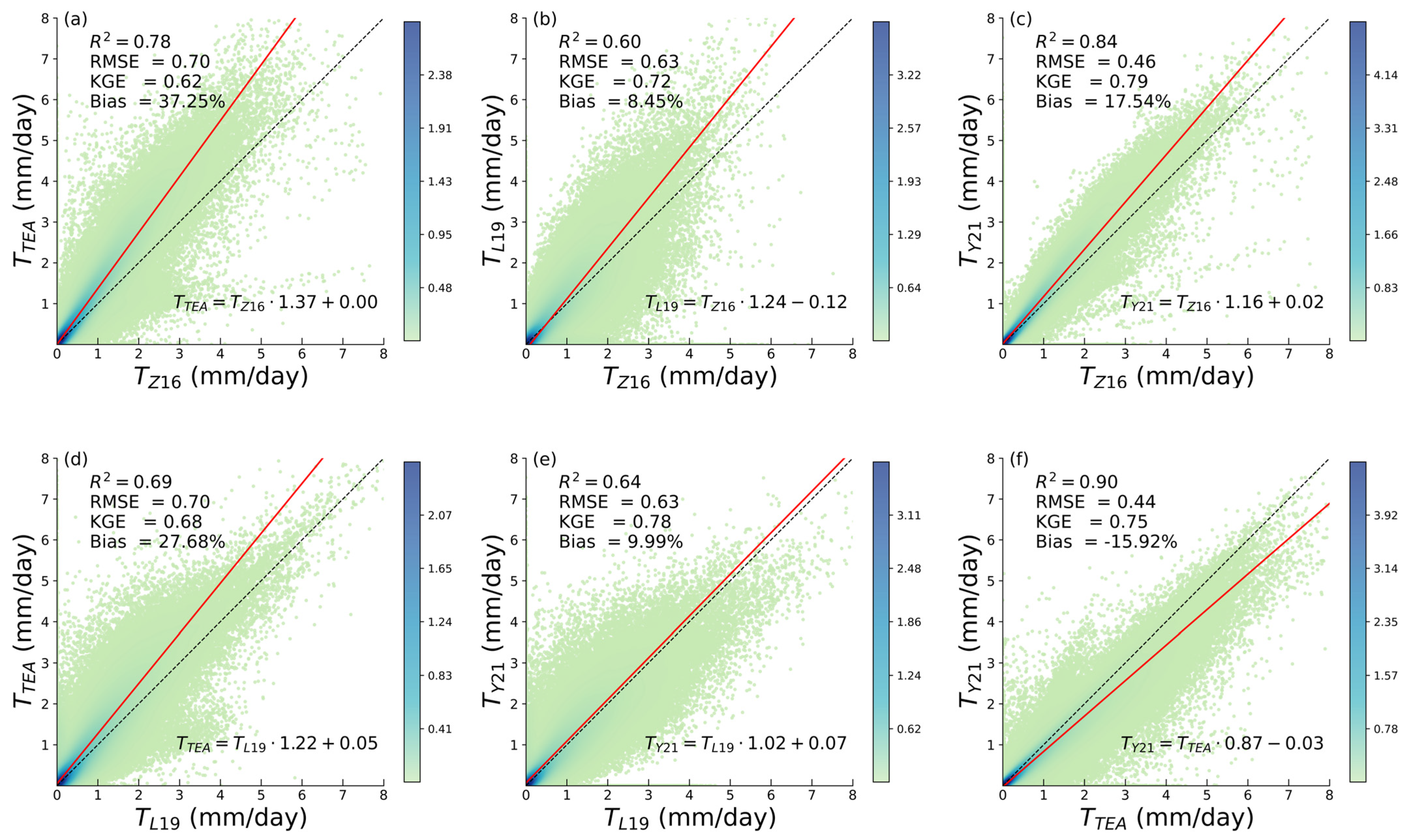
We first compared the consistency of the four methods in estimating daily T (Figure 2). Overall, T estimations derived from TEA demonstrated the highest consistency with those of Y21, with an R² of 0.90, RMSE of 0.44 mm d⁻¹, and KGE of 0.75 (Figure 2f). The daily T results from Z16 seemed to have reasonable consistency with Y21, as indicated by R² = 0.84, KGE = 0.79, and RMSE = 0.46 mm d⁻¹. A relatively lower consistency was observed between Z16 and TEA and between L19 and TEA (Figure 2a,d). According to the bias metric, we found TEA generally produced higher estimates of daily T, followed by Y21. In contrast, Z16 yielded a slight underestimation of daily T values among the four methods.

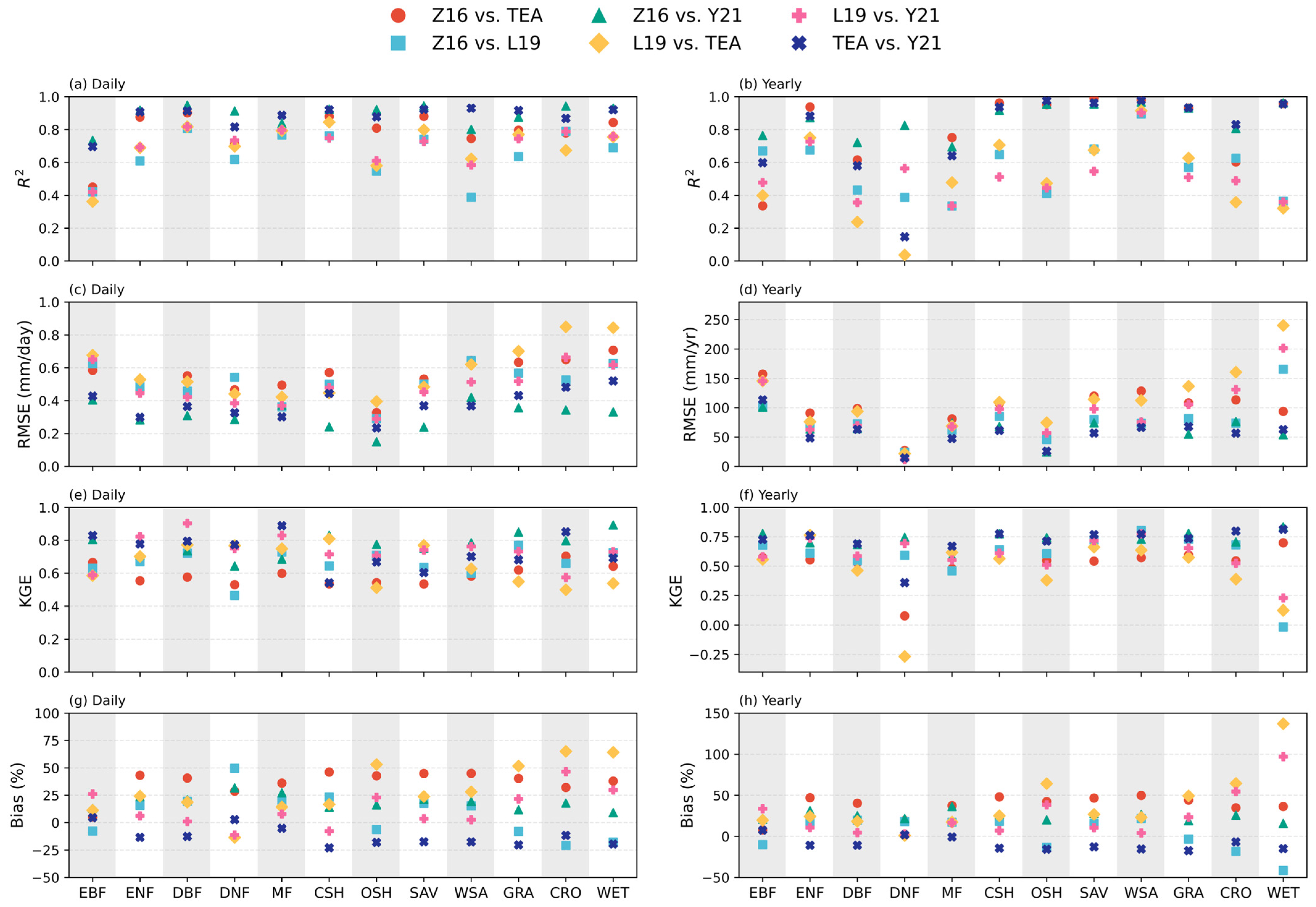
Across the 12 ecosystem types (Figure 3a,c,e,g), the four methods showed the highest consistency in DBF, with R² ranging from 0.81 to 0.95, RMSE from 0.36 to 0.55 mm d⁻¹ and KGE from 0.58 to 0.90. MF had the second-best consistency in daily T estimation, with R² between 0.77 and 0.89, RMSE between 0.30 and 0.49 mm d⁻¹, and KGE between 0.60 and 0.89. By contrast, the lowest consistency was observed in EBF (R² = 0.36–0.70, RMSE = 0.40–0.68 mm d⁻¹, and KGE = 0.59–0.83), which suggests that EBF has a highly complex canopy structure and different ET partitioning methods have poor adaptability in EBF. Overall, the four methods had better consistency in shrublands (CSH and OSH), followed by forests (except for EBF). Greater discrepancies were found in grasslands (WSA), CRO and WET. In terms of the four methods, TEA and Y21 demonstrated the highest consistency in daily T estimates across most ecosystem types, even though the T values from TEA were always higher than those from Y21. However, at CSH, OSH, CRO, and WET, the T results from Y21 agreed most closely with those of Z16. TEA tended to yield an overestimation of T across all ecosystem types, indicating that its T and T/ET estimations were substantially higher than those of the other methods. Y21 generally produced higher T estimates than Z16 and L19. Daily T values from L19 were also higher than those from Z16 in most ecosystem types, whereas in EBF, GRA, CRO, and WET, the T values from Z16 exceeded those of L19. These findings indicate that TEA generally had the highest T and T/ET estimates, followed by Y21, while L19 and Z16 produced the lowest T and T/ET values.

3.1.2. Comparison of the Four ET Partitioning Methods at Annual Scale

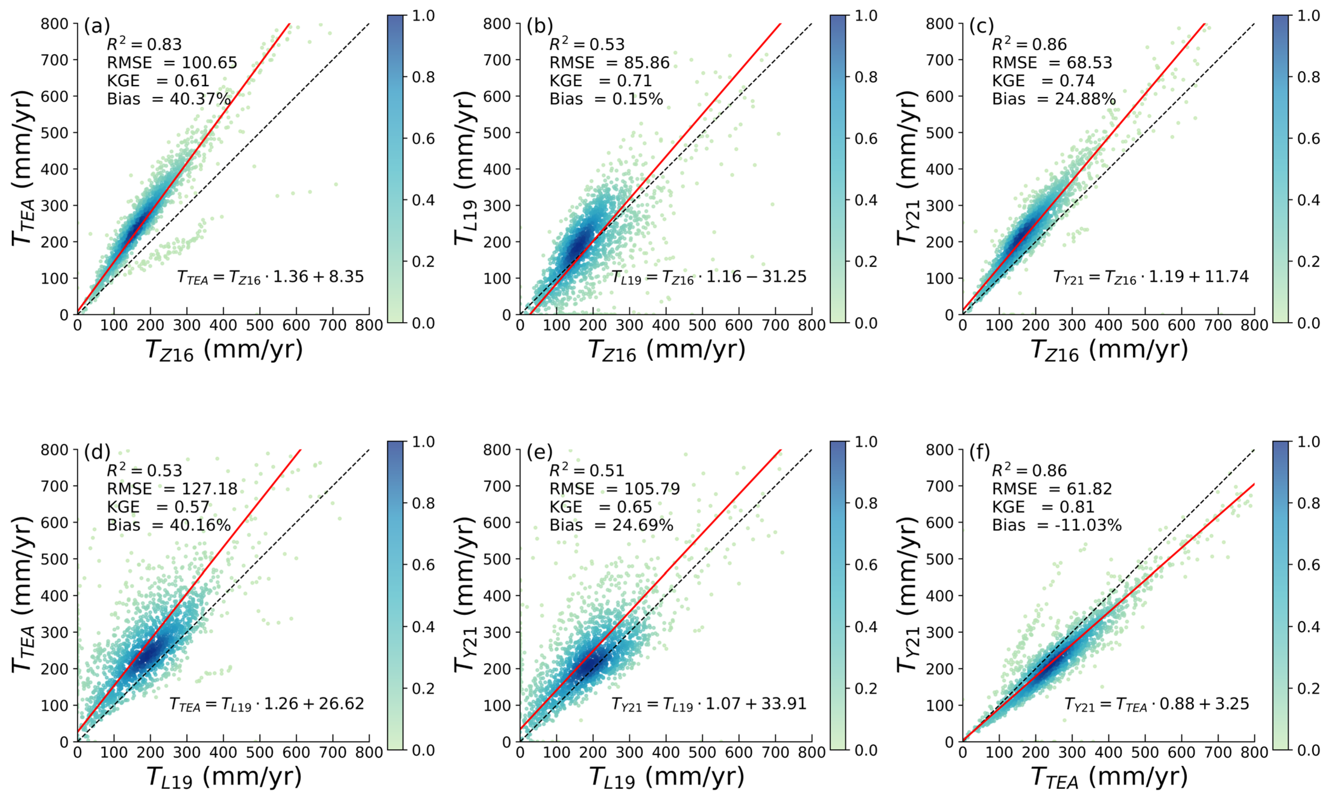
Compared to the daily-scale results (Figure 2 and Figure 3), the consistency of T estimated from the four methods showed slight degradation at the annual scale (Figure 4), evidenced by decreased R² (0.51–0.86) and KGE values (0.57–0.81), alongside increased RMSE and bias values. Specifically, the R² and KGE values between TEA and L19 declined to 0.53 and 0.57, respectively. In comparison, annual T results from Z16 and Y21 showed relatively better consistency than daily T, with R² of 0.86 and KGE = 0.74, despite a slight overestimation of T from Y21 during the high value range of annual T (Figure 4c). The temporal dynamics of annual T estimated by L19 diverged more significantly from the other three methods, with R² values ranging from 0.51 to 0.53 and notably lower than other results (R² = 0.83–0.86). Furthermore, compared to Z16, L19 and Y21, the overestimation of T by TEA becomes more pronounced. However, at the BR-Sa1 (EBF) site, TEA significantly underestimates annual T, ranging from 308 to 357 mm yr⁻¹ (0.30–0.32 for T/ET), which is considerably lower than the annual T estimated by the other three methods (Figure 4a,d,f).

The differences among the four ET partitioning methods were more pronounced at the annual scale across the 12 ecosystem types (Figure 3b,d,f,h). Different from the daily-scale results, all four methods showed higher consistency in WSA, evidenced by an R² of 0.90–0.98 and KGE of 0.57–0.80, followed by ENF (R² = 0.68–0.94, KGE = 0.55–0.76) and SAV (R² = 0.55–0.99, KGE = 0.54–0.77). Conversely, poor agreement was observed in DNF, WET, SAV, GRA, CSH and OSH. In DNF, the comparison results were highly uncertain (R² = 0.04–0.83, KGE = −0.27–0.75), which is due to the limited site-year observations with only two sites. In WET, SAV, GRA, CSH and OSH, the poor agreement primarily originates from the L19 methods, as their results exhibit substantial uncertainty in capturing the interannual variations in T compared to the other three methods. In summary, the highest consistency of annual T among the four methods was found in shrublands, followed by grasslands and forests. In addition, TEA and Y21 overestimated annual T across all ecosystem types. Z16 and L19 had relatively similar magnitudes of annual T, with L19 producing higher annual T values than Z16 in forests, shrublands, and SAV, while Z16 exceeded L19 in EBF, OSH, CRO, GRA, and WET.

3.1.3. Validation by the Sap Flow Data

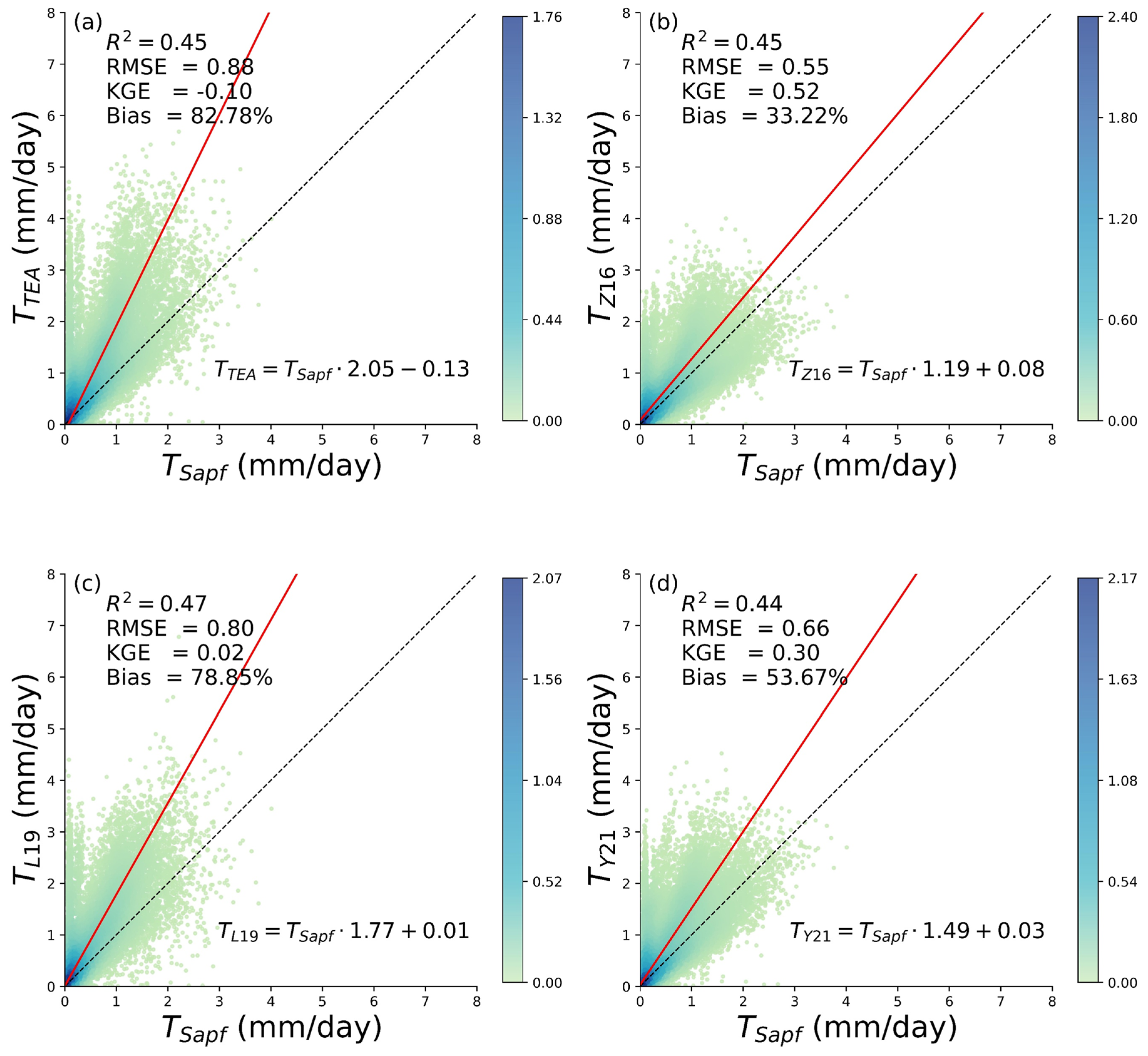
The daily T estimates from the four ET partitioning methods were further evaluated by sap flow data at 15 sites (Figure 5). The validation results showed that Z16 achieved the best performance, with an R² of 0.45, RMSE of 0.55 mm d⁻¹, and KGE of 0.52. Comparatively, Y21 ranked second, with R² = 0.44, RMSE = 0.66 mm d⁻¹, and KGE = 0.30. L19 and TEA demonstrated the lowest accuracy, with an R² of 0.47 and 0.45, and KGE of 0.02 and −0.10, respectively. Moreover, all four methods systematically overestimated daily T, with Z16 showing the smallest overestimation (bias = 33.22%) and TEA having the largest positive bias (bias = 82.78%). The systematic overestimation of daily T from the four methods is partly attributed to the fact that the sap flow data used in this study were only observed on trees. The absence of measurements on understory vegetation and tree density (or coverage) in those sites likely led to lower daily T values from sap flow data compared to the estimates from the other four methods.

To further comprehensively evaluate the model performance, a normalized Taylor diagram was employed to simultaneously visualize the correlation coefficient (R), centered root mean square error (CRMSE), and normalized standard deviation (SD) of the four methods against the sap flow data (Figure 6). The diagram clearly illustrates that while all four methods exhibited comparable temporal correlations (R ranging from 0.66 to 0.68), they differed substantially in capturing the amplitude of daily T variations. Z16 emerged as the most accurate method, positioned closest to the observation reference point with the lowest CRMSE (0.87) and an SD closest to 1.0 (1.12). Conversely, TEA was located furthest from the reference, displaying a highly inflated SD (1.65) and the largest CRMSE (1.23). This indicates a severe overestimation of the variance, perfectly aligning with its highest positive bias (82.78%) shown in Figure 5. Y21 and L19 exhibited intermediate performance. These multidimensional spatial distributions in the Taylor diagram robustly corroborate the scatter plot statistics, firmly establishing Z16 as the optimal choice for daily T estimation.

To account for the potential measurement and upscaling errors in the sap flow data, the statistical robustness of the overall validation was further assessed using a Monte Carlo simulation. As presented in

Table 2. Validation performance of the four ET partitioning methods against sap flow data at the 15 SAPFLUXNET sites using a Monte Carlo simulation. Values in parentheses represent the 95% confidence intervals derived from 1000 iterations with a 15% random noise.

Method	R2 (95% CI)	RMSE (mm d−1) (95% CI)	KGE (95% CI)	Bias (%) (95% CI)
Z16	0.45 (0.43–0.43)	0.55 (0.57–0.57)	0.52 (0.51–0.52)	33.22 (32.78–33.66)
Y21	0.44 (0.42–0.42)	0.66 (0.67–0.68)	0.30 (0.29–0.31)	53.67 (53.16–54.14)
L19	0.47 (0.44–0.45)	0.80 (0.81–0.81)	0.02 (0.02–0.04)	78.85 (78.17–79.53)
TEA	0.45 (0.42–0.43)	0.88 (0.89–0.89)	−0.10 (−0.10–−0.08)	82.78 (82.25–83.34)

, the extremely narrow 95% confidence intervals of the four evaluation metrics demonstrate that the comparative performance of the ET partitioning methods remained stable against data uncertainties. Specifically, Z16 consistently maintained the highest accuracy with KGE values narrowly ranging from 0.51 to 0.52, whereas TEA exhibited the largest systematic overestimation with Bias ranging from 82.25% to 83.34%. This rigorous uncertainty analysis confirms that the significant performance gap between Z16 and the other methods—as well as the method rankings established in the scatter plots (Figure 5) and the Taylor diagram (Figure 6)—is statistically sound and unaffected by the inherent uncertainties of the 15 validation sites.

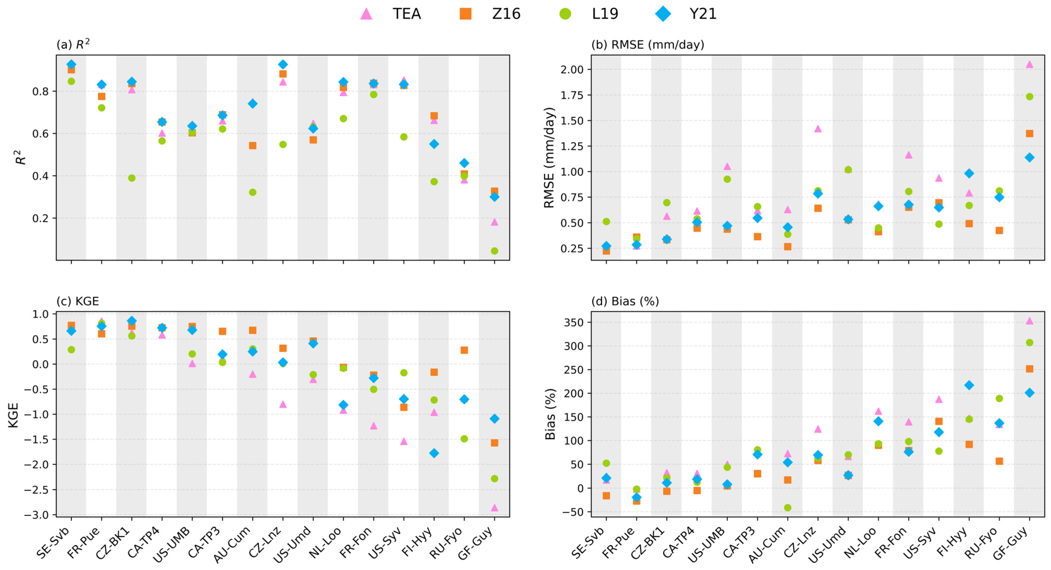
We conducted a detailed evaluation of the four methods on daily T estimation at each sap flow site. As shown in Figure 7, the four methods performed consistently well at SE-Svb (ENF), FR-Pue (EBF), CZ-BK1 (ENF), and CA-TP4 (ENF) (R² = 0.39–0.93, KGE = 0.29–0.86), moderately at sites like US-UMB (DBF) and CA-TP3 (ENF) (R² = 0.60–0.69, KGE = 0.01–0.75), and poorly at sites including GF-Guy (ENF), RU-Fyo (ENF), and FI-Hyy (ENF). Regarding the overall performance of the four methods, Y21, TEA, and Z16 achieved relatively high R² values at most sites, indicating their good capability in capturing the temporal dynamics of daily T. In contrast, L19 consistently yielded the lowest R² values across most sites, reflecting its comparatively poorer performance in representing temporal variations in T. According to other metrics (RMSE, KGE, and bias), Z16 performed the best, with the highest KGE values and the lowest RMSE and bias values among the four methods. This is consistent with the conclusion drawn in Figure 5, confirming Z16 as the optimal choice of ET partitioning, followed by Y21. The TEA method showed notably lower KGE values, along with the highest RMSE and bias, which may be attributed to limitations of the machine learning algorithms in accurately capturing temporal dynamics. In contrast, the greater consistency of the Y21 method compared to TEA can be largely attributed to the annual variability of the parameter g₁. By estimating g₁ annually using the OLS regression model based on the inverted Penman–Monteith equation, the Y21 method dynamically captures the interannual physiological adaptations of canopy water-use strategies to varying environmental conditions. This explicit parameterization of annual flexibility avoids the temporal rigidity typical of data-driven machine learning models trained on specific periods, thereby maintaining a more robust temporal consistency with sap flow dynamics. Additionally, the significant differences in the performance of the four ET partitioning among the 15 sites suggest that their accuracy is influenced by many factors such as the quality of observation data, canopy structure and plant physiological traits, as well as the heterogeneity of site environments.

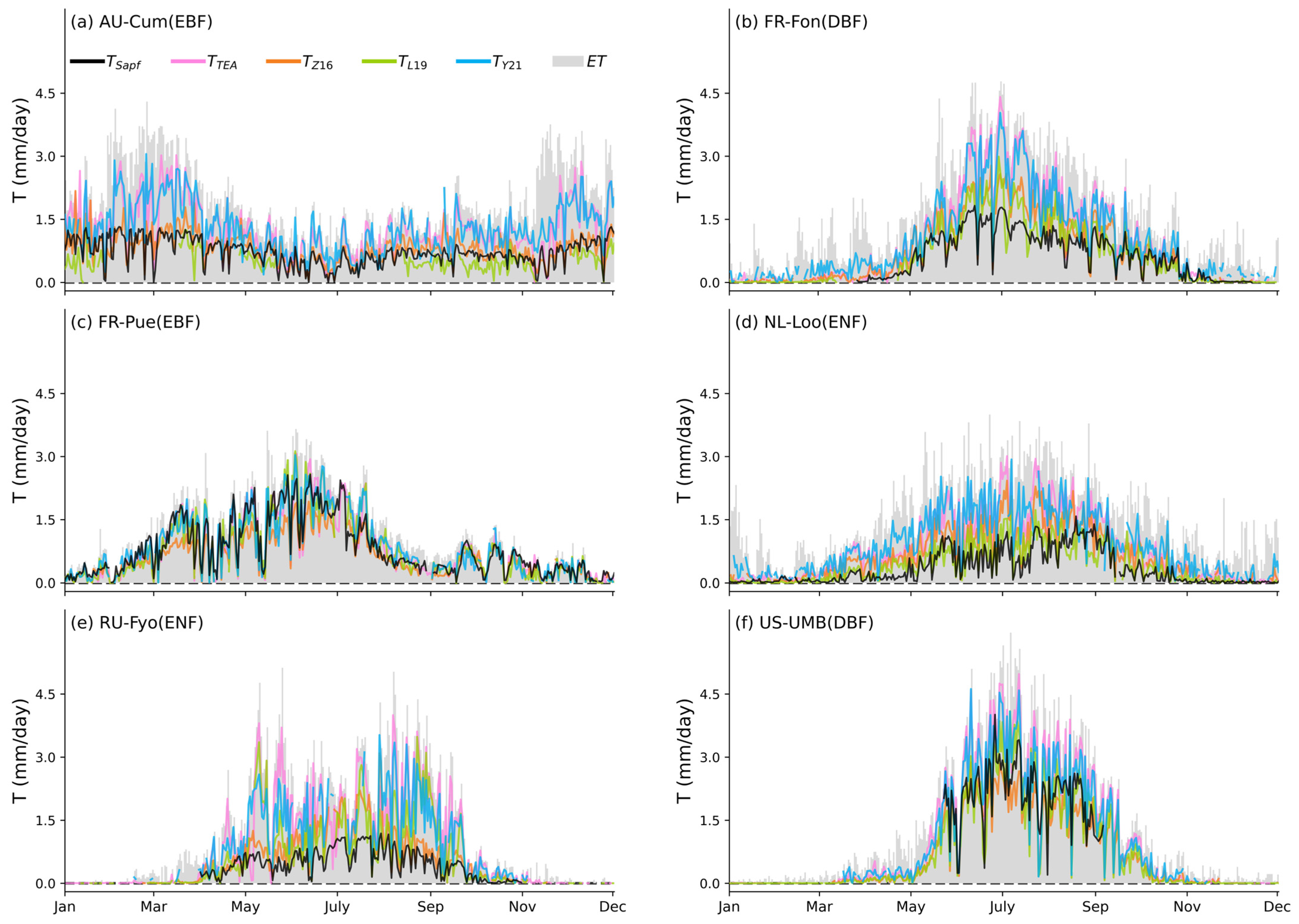
We compared the seasonal trajectories of T estimated by the four methods with sap flow-based T across six sites (AU-Cum, FR-Fon, FR-Pue, NL-Loo, RU-Fyo, and US-UMB, Figure 8). The results show that all four methods were able to reproduce the seasonal cycle of T, with peak values occurring during the peak growing season and their magnitudes constrained by ET. However, notable discrepancies were observed among the methods in the estimated T magnitude. TEA and Y21 generally produced significantly higher values, which approached the range of ET, while Z16 and L19 yielded lower values and aligned more closely with sap flow curves, especially during shoulder seasons. These site-level trajectories indicate broad seasonal consistency across the four methods but non-negligible differences in daily T magnitude.

3.2. Spatial Patterns and Long-Term Trends of T and T/ET

3.2.1. Spatial Distribution of T and T/ET

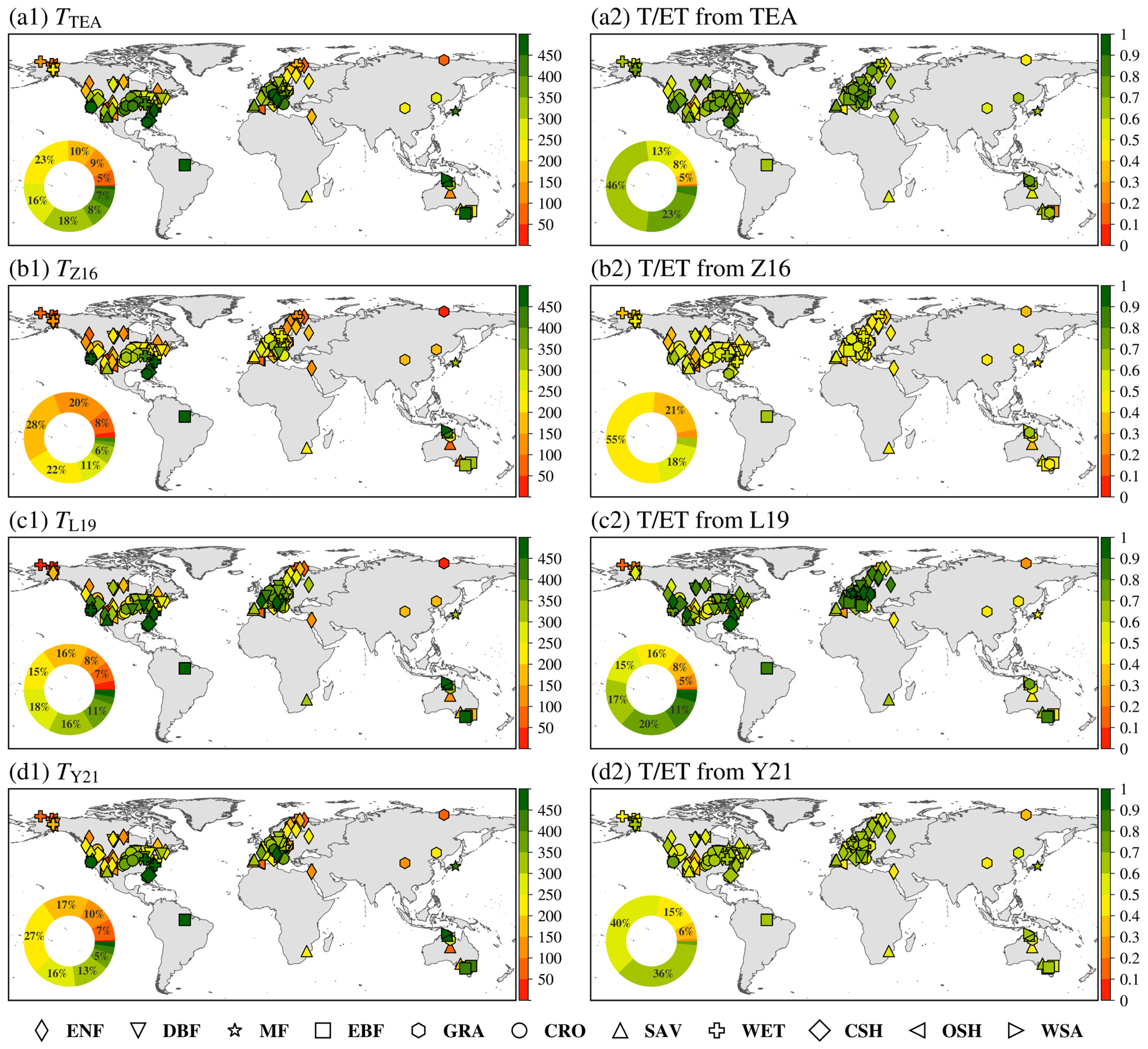
Figure 9 illustrates the spatial patterns of multi-year mean T and T/ET estimated by the four ET partitioning methods (Figure 9). Overall, the four methods exhibited consistent spatial patterns of annual T across the globe. High annual T values were predominantly observed in the humid low- to mid-latitude regions, such as eastern North America and western Europe where forest and cropland vegetation has strong photosynthetic activity. In contrast, low annual T values were widely distributed in high-latitude regions and arid areas in mid- to low-latitude zones, e.g., northern Europe, central North America, and central Australia (Figure 9a1–d1). These areas are characterized by sparse vegetation cover and consequently low transpirational water loss. Despite the consistent spatial patterns, significant discrepancies appeared in the magnitude of annual T. Specifically, the global mean annual T estimated by TEA was the highest at 294 ± 150 mm yr⁻¹, followed by L19 and Y21 with mean values of 278 ± 148 mm yr⁻¹ for L19 and 262 ± 134 mm yr⁻¹, respectively. Z16 had the lowest global mean annual T, only 213 ± 116 mm yr⁻¹. This result aligns with the validations based on sap flow data (Figure 5). Across the 201 sites, approximately 40% and 38% of the sites exhibited T values exceeding 300 mm yr⁻¹ for TEA and Y21, respectively. By contrast, annual T from Z16 and L19 fell primarily within the ranges of 150–300 mm yr⁻¹ (56%) and 200–350 mm yr⁻¹ (51%), respectively.

The spatial distribution of T/ET (Figure 9a2–d2) was generally consistent with that of annual T. High annual T/ET values were predominantly found in humid regions at low-to-middle latitudes, while low values were concentrated in high-latitude areas and the arid/semi-arid regions at middle latitudes. Notably, due to the overall lower annual T estimates from Z16 compared to the other three methods, the mean annual T/ET values (0.45 ± 0.07 for Z16) were significantly lower (0.63 ± 0.12 for TEA, 0.61 ± 0.18 for L19, and 0.56 ± 0.09 for Y21). Only 43 sites (21%) showed mean annual T/ET exceeding 0.5 under the Z16 method—considerably fewer than those under the other three methods (173 sites and 86% for TEA, 139 sites and 69% for L19, and 157 sites and 78% for Y21). Furthermore, both Z16 and Y21 estimated maximum annual T/ET values below 0.8, whereas TEA and L19 yielded annual T/ET estimates above 0.8 at 7 sites (3%) and 32 sites (16%), respectively.

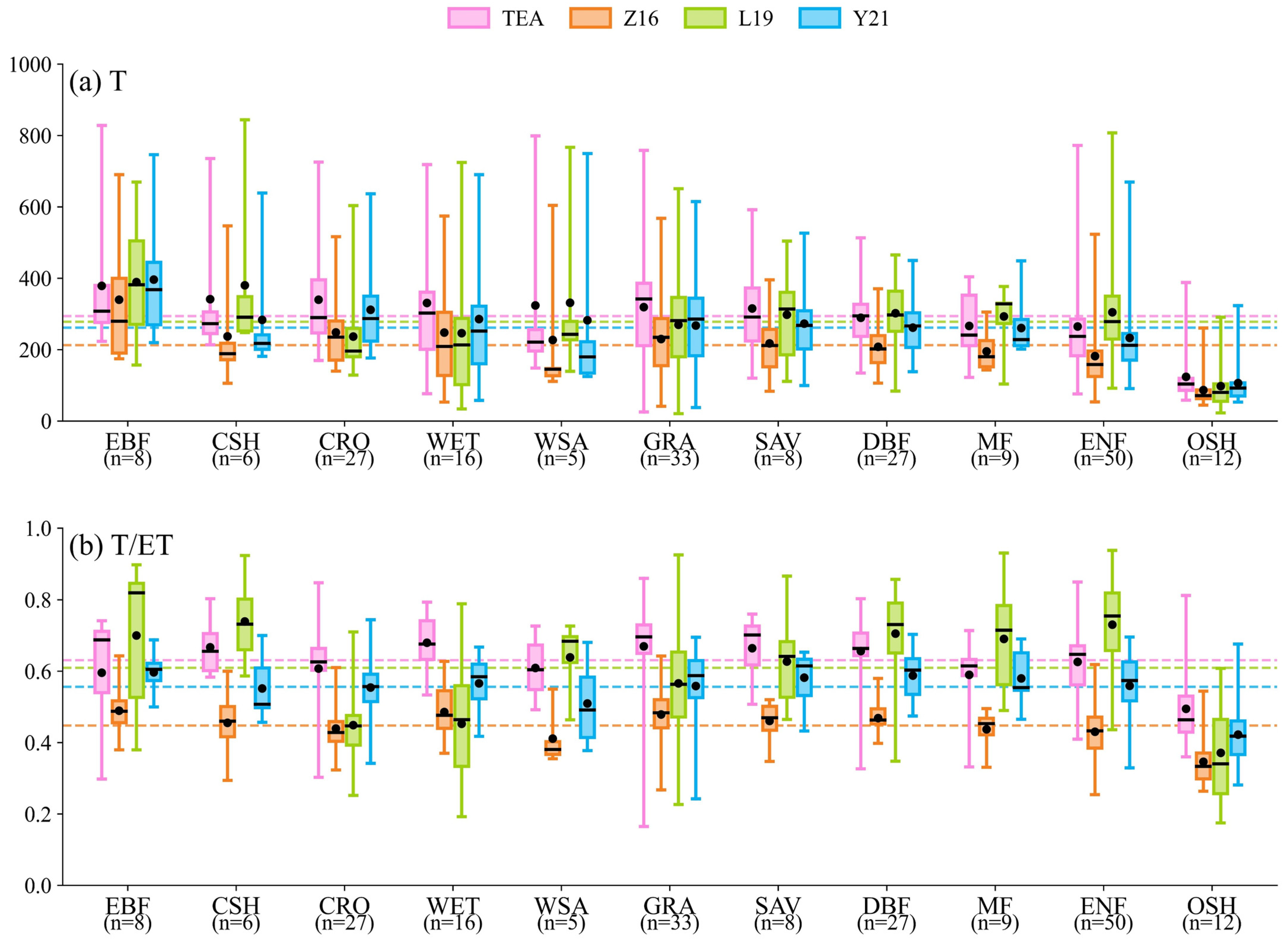
Figure 10 further compares the annual T and T/ET values across different ecosystem types, revealing the significant regulation of vegetation characteristics on ET partitioning. EBF exhibited the highest annual T for all four methods, with mean values ranging from 340 (Z16) to 396 mm yr⁻¹ (Y21), whereas OSH showed the lowest annual T values (mean: 87 for Z16 –124 mm yr⁻¹ for TEA). For other ecosystem types, notable discrepancies were observed among the TEA, Z16, and Y21 methods when compared with L19. TEA, Z16, and Y21 consistently estimate slightly lower annual T for CRO, WET, and CSH than for EBF, while grassland (WSA, SAV and GRA) exhibited moderate annual T values, whereas ENF, MF, and DBF were somewhat higher than OSH. By comparison, L19 yielded markedly higher annual T for CSH, WSA, ENF, and DBF relative to other vegetation types, such as MF, GRA, and CRO.

The distribution of T/ET across ecosystem types varied substantially among the four methods (Figure 10b). All four methods consistently estimated the lowest annual T/ET for OSH. CRO generally also exhibited relatively low T/ET, which may be associated with factors such as agricultural irrigation and exposed soil. The ecosystem type with the higher annual T/ET differed depending on the method. TEA showed higher T/ET for WET and GRA than for EBF and MF, Z16 indicated that T/ET at the EBF and WET sites was higher than that of the WSA, MF, and ENF sites. Y21 suggested that T/ET at the CSH, ENF, and DBF sites exceeded that of grassland and WET, whereas L19 revealed that EBF and DBF had markedly higher annual T/ET than WSA and CSH. The pronounced inconsistency in T/ET across ecosystems among the four methods demonstrates the substantial structural and parametric uncertainties in current ET partitioning approaches. This further underscores the necessity for direct measurements of ET components (e.g., T) and ET partitioning method development.

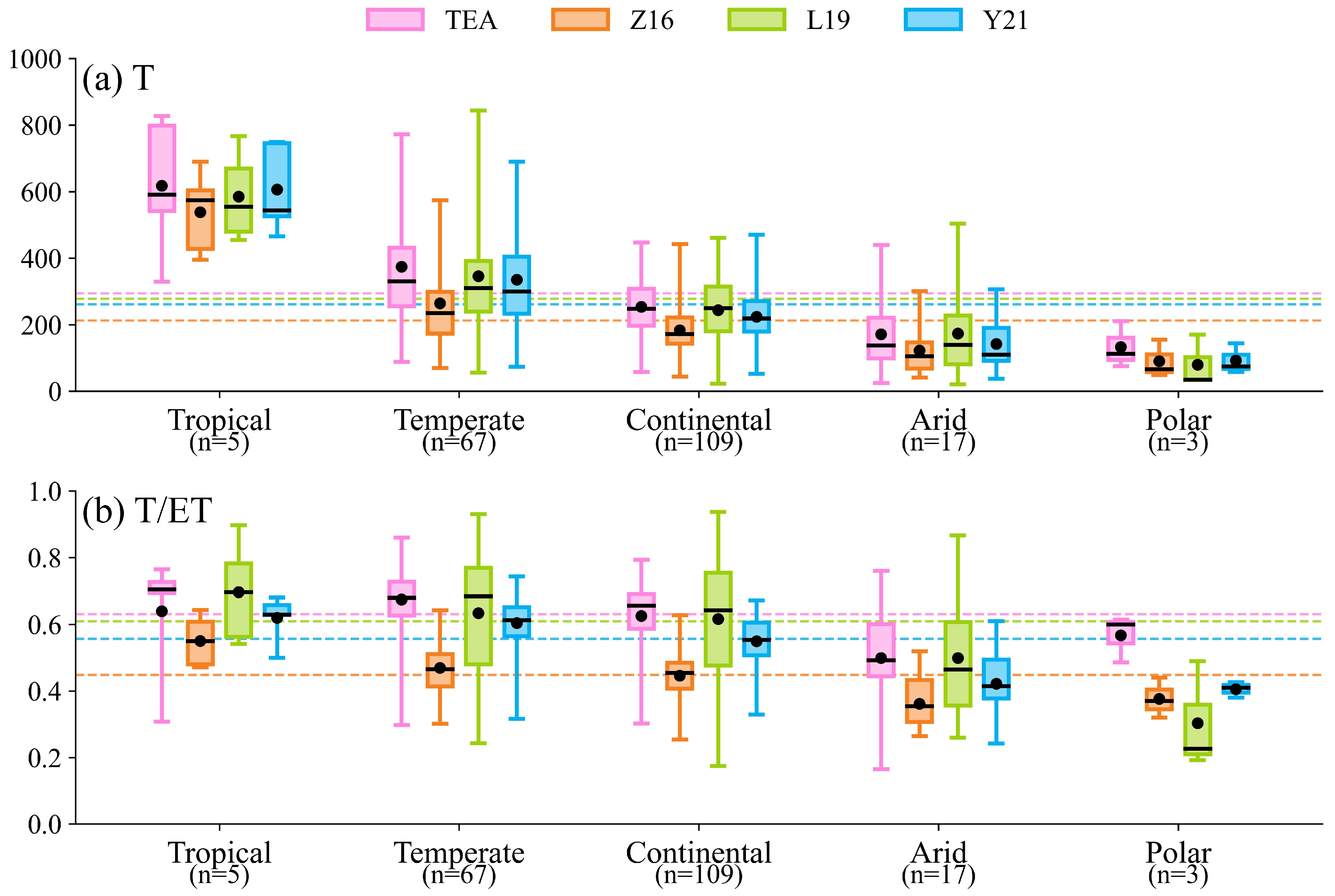
Beyond ecosystem-specific responses, background climate regimes exert fundamental control over ET partitioning. To quantitatively isolate these climatic constraints, Figure 11 illustrates the variations in annual T and T/ET across the five primary Köppen–Geiger climate zones. As expected, all four methods captured a distinct climatic gradient in annual T. The highest transpirational water loss was consistently estimated in tropical environments, with mean annual T ranging from 538 mm yr⁻¹ (Z16) to 618 mm yr⁻¹ (TEA). Conversely, the severe energy constraints of polar regions resulted in the lowest T estimates, dropping to mean values between 80 (L19) and 133 mm yr⁻¹ (TEA). However, in intermediate climates (temperate and continental), model divergence became significantly more apparent. While TEA, L19, and Y21 produced relatively comparable and higher T estimates in these regions, Z16 systematically yielded the lowest values, highlighting the differing sensitivities of these models to moderate climate forcing.

Evaluating the T/ET ratio across these climate zones (Figure 11b) further exposed method-specific uncertainties. Arid and polar zones generally exhibited the lowest partitioning ratios across all methods, reflecting the respective dominance of bare soil evaporation under water deficit and the suppression of vegetation transpiration under extreme cold. Nevertheless, the absolute magnitude of T/ET varied remarkably. Z16 maintained the most conservative estimates across the global climate spectrum, spanning from a minimum of 0.36 in arid zones to a maximum of 0.55 in tropical regions. In stark contrast, TEA and L19 estimated considerably higher T/ET ratios, particularly in the humid tropical and temperate zones. These climate-driven disparities emphasize that structural differences among ET partitioning models are strongly amplified by macroclimatic conditions, reinforcing the need for regionally calibrated approaches rather than universally applied algorithms.

3.2.2. Interannual Trends of Annual T and T/ET

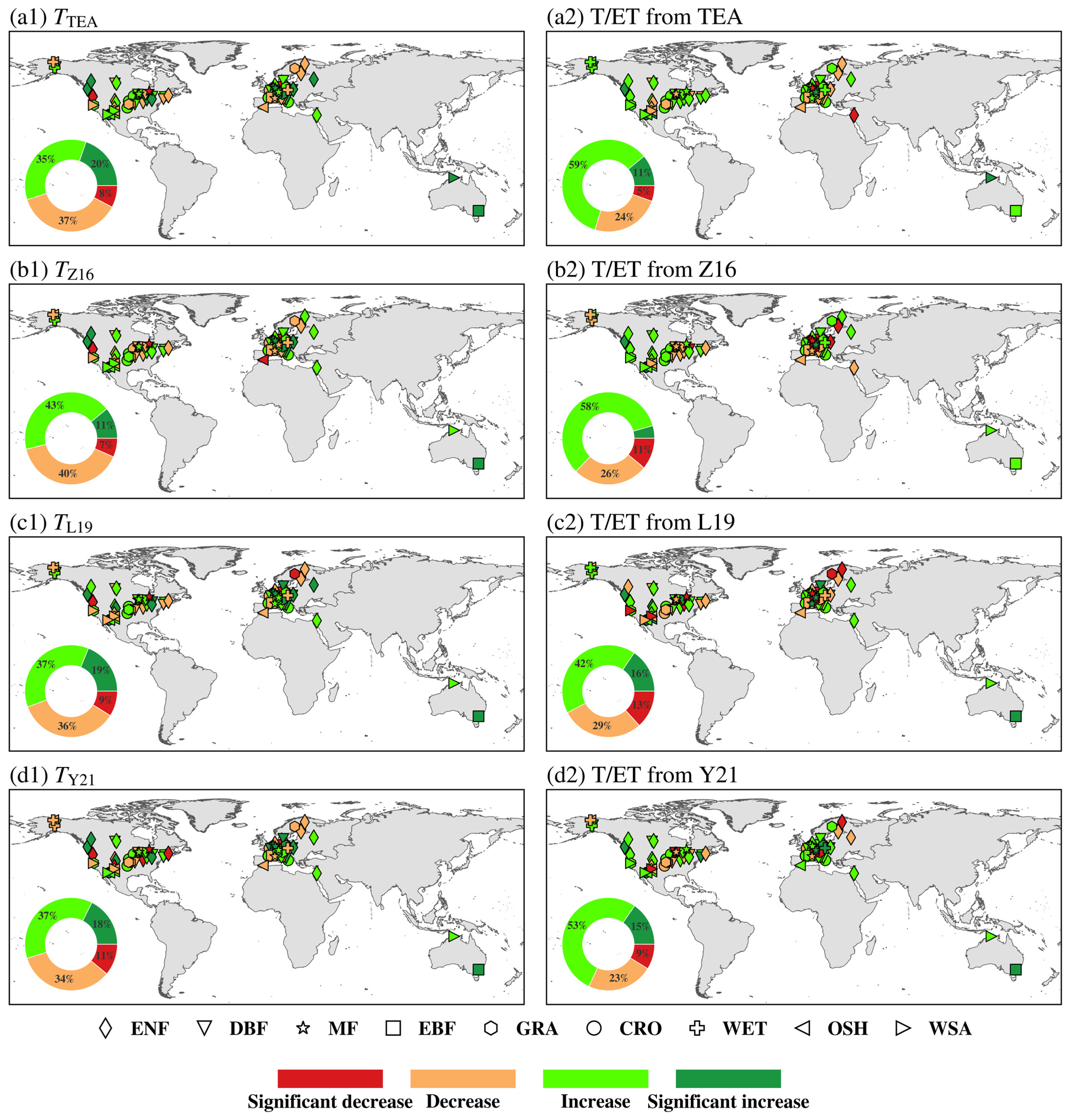
To evaluate the consistency among the four ET partitioning methods, we analyzed the interannual trends of both T and T/ET at 91 flux sites with at least 10 years of measurements. All the four methods estimated an increasing trend in annual T at the global scale (Figure 12a1–d1), although the magnitudes of increase varied. Among them, L19 showed the largest increasing trend (0.83 mm yr⁻²), whereas Z16 produced the smallest (0.33 mm yr⁻²). Nevertheless, the spatial pattern of T trends exhibited high heterogeneity and strong site dependence. Among the 91 sites, all four methods indicated that over half of the sites (50 sites, 55%) had an increasing trend in annual T, with 10–18 sites (11–20%) exhibiting statistically significant increasing trend. These sites are primarily distributed across DBF, ENF, MF, and GRA vegetation types. In contrast, 6–10 sites (6–11%) show significant decreasing trends, scattered among ENF, MF, and OSH. Across the nine ecosystem types examined, annual T displays decreasing trends only in WET and OSH. In most ecosystem types, such as CRO, WSA, and forest types (DBF, ENF, and EBF), all four methods consistently estimated increasing trends in annual T, with the most pronounced rises observed in WSA and EBF. For MF, discrepancies exist among the methods, in which TEA and Z16 suggested a decreasing trend, whereas L19 and Y21 indicated an increase.

Similarly, the interannual trend in T/ET generally indicated an upward tendency, albeit with a much smaller magnitude (ranging from 0.0015 to 0.0019 yr⁻¹) (Figure 12a2–d2). This suggests that annual T/ET exhibits a relatively conservative behavior. According to all four methods, more than half of the sites (52–64 sites, 57–70%) showed an increasing trend in annual T/ET. However, only a limited number of sites (4–14 sites, 4–15%) displayed statistically significant increases, fewer than those observed for annual T. And these sites were predominantly located in DBF and ENF. In contrast, significantly decreasing trends were observed at 5–12 sites (5–13%), which exceeded the number of sites with significant declines in annual T, and they were mainly distributed across GRA and MF. Across almost all ecosystem types, T/ET consistently exhibited an increasing trend. Notable divergence occurred in WET, WSA, and MF, where Z16 and L19 suggested a declining trend, different from the results of TEA and Y21. This widespread increasing trend in T/ET, especially in croplands (CRO), implies a gradual shift toward higher ecosystem water use efficiency, which introduces new variables for regional agricultural water allocation.

3.3. Interannual Coupling Between GPP, T and ET

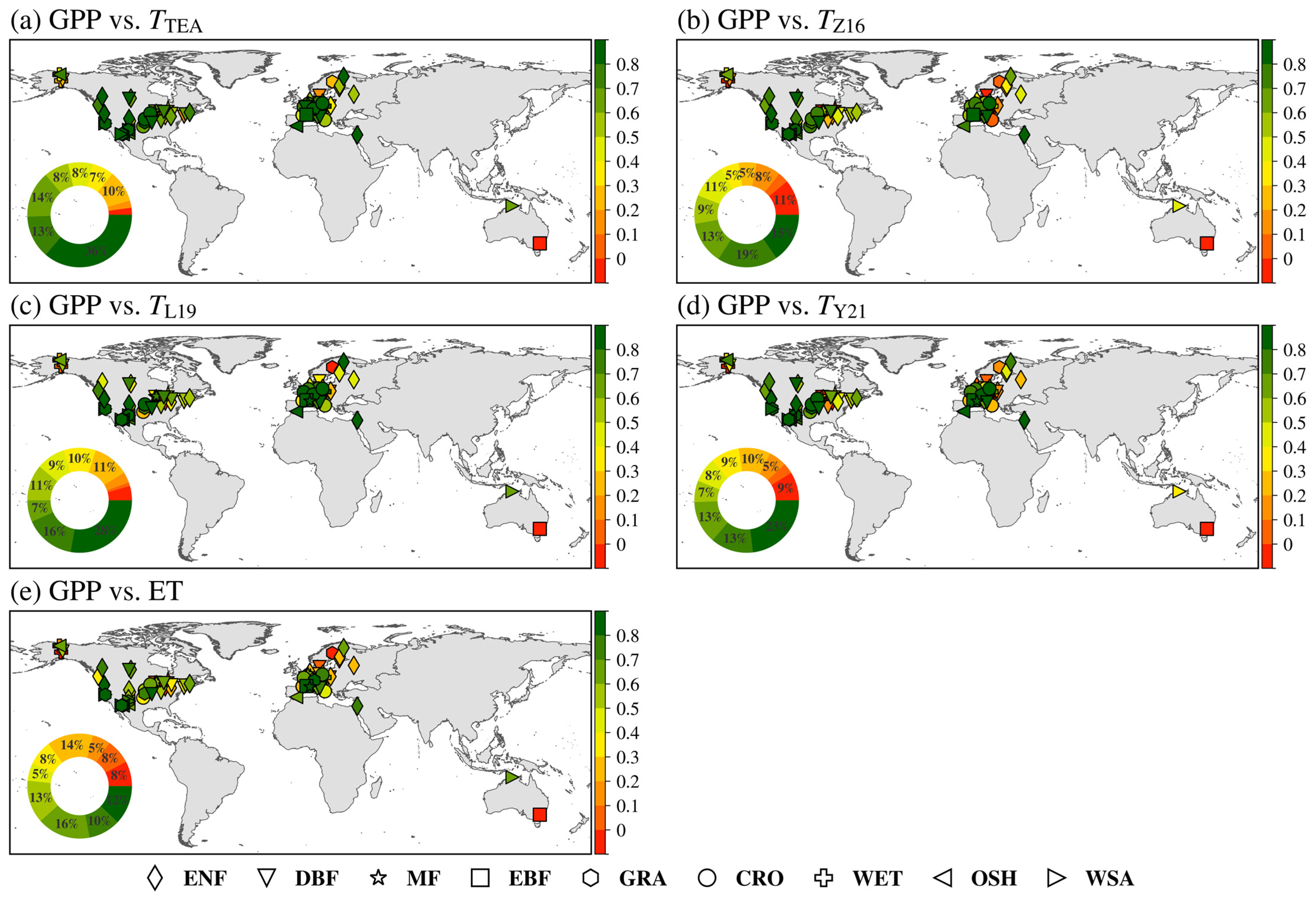
We additionally compared the correlation between detrended annual GPP and T from the four methods and between GPP and ET by using the Pearson correlation coefficients (r). Figure 13 illustrates the spatial distributions of these correlations at 91 sites. Overall, the interannual correlations between GPP and T (r = 0.49 for Z16—0.61 for TEA) were consistently stronger than those between GPP and ET (r = 0.44), indicating that the inherently strong coupling between ecosystem photosynthesis and transpiration processes. In most sites (81–89 sites, 89–97%), GPP was positively correlated with T, whereas the positive correlation between GPP and ET was found at 84 sites (92%). Moreover, nearly half of the sites (43–58 sites, 47–63%) exhibited a strong positive correlation (r > 0.6) between GPP and T, distributed across all ecosystem types. Only a few sites showed negative correlations between GPP and T, including AU-Tum (EBF), IT-Tor (GRA), and US-Oho (DBF), indicating a strong site dependence. Across all ecosystem types, GPP always had positive correlations with both T and ET. And in ecosystem types such as WSA, OSH, CRO, and GRA, the correlations between GPP and both ET and T were relatively strong, while in WET, EBF, and DBF, the positive correlation between GPP and T was comparatively weak.

4. Discussion

4.1. Performance Evaluation and Methodological Limitations of Four ET Partitioning Methods

The four ET partitioning methods showed consistent seasonal dynamics in transpiration (Figure 2). However, they differed significantly in the magnitude of T estimates. To date, no consensus has been reached in the published literature regarding which ET partitioning method based on EC data is the most accurate. However, using the sap flow data from 15 sites as an independent benchmark, Z16 was identified as the best ET partitioning method in this study, followed by Y21, while TEA was considered the poorest (Figure 5).

Apart from the inherent uncertainties associated with the EC measurements (e.g., underestimation of fluxes, energy closure issues, uncertainties in GPP estimation) and the neglect of canopy interception evaporation, the differences among the four ET partitioning methods primarily stem from model assumptions, model structure and parameterization. Here, we discussed the advantages and limitation of the four methods and the possible reasons or sources of uncertainty.

Both the model intercomparisons and sap flow validation results indicated that TEA overestimates T, although it effectively captured the temporal dynamics of T (R² = 0.45, while KGE = −0.10). This is mainly attributed to the high bias of TEA (Bias = 82.78%, Figure 5). TEA employs RF model to predict the temporal dynamics of WUE (i.e., GPP/T) across all temporal scales, thereby estimating T. This method is based on the coupled carbon–water relationship, has minimal assumptions and is entirely data-driven without additional prior knowledge [16,28,34]. However, an error of this magnitude requires a thorough reevaluation of its two core training parameters: the CSWI threshold and the prediction percentile.

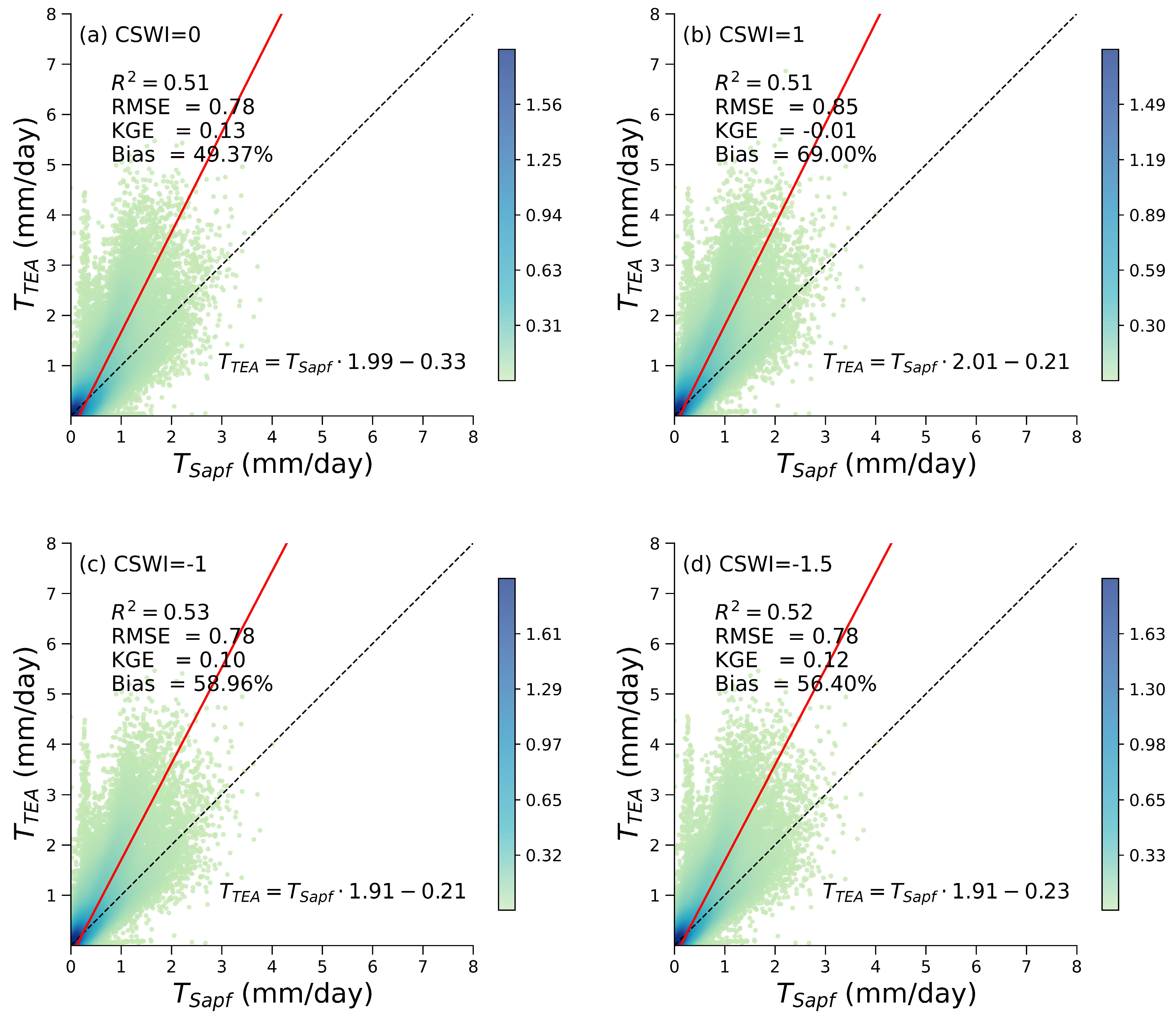
The TEA algorithm relies on the CSWI threshold to isolate periods with dry surfaces and active vegetation, assuming that ET is dominated by T (i.e., T ≈ ET) to construct the RF training dataset. To evaluate its impact, we conducted a sensitivity analysis using different CSWI limits (1, 0, −1, and −1.5 mm) under the default 75th percentile (Figure 14). The results showed that while the temporal correlation remained stable (R² ranging from 0.51 to 0.53), the Bias and KGE fluctuated. Although adjusting the CSWI to 0 mm or −1.5 mm reduced the bias to 49.37% and 56.40%, respectively (compared to the original 82.78% at CSWI = −0.5), the overestimation remained substantial. This indicates that modifying the CSWI filter alone is insufficient. As explicitly warned by Nelson et al. [28], ecosystems with persistent soil evaporation or sparse vegetation (such as wetlands or drylands) inherently contain persistent evaporation in the training dataset, denoted as E_train. This fundamentally affects the random forest training process. Because the RF model is trained to characterize the WUE dynamics based on the assumption that T ≈ ET during the filtered periods, the presence of persistent E_train means the target variable (eWUE = GPP/ET) is systematically lower than the true biological WUE (GPP/T). Consequently, the RF model learns this biased, underestimated WUE relationship. When the trained model predicts WUE for the entire time series, the underestimated WUE predictions inevitably lead to a systematic overestimation of T (since T = GPP/WUE). The CSWI filter, which primarily removes periods immediately after rainfall, struggles to eliminate this persistent background evaporation, inevitably leading to a systematic overestimation of T when using default settings.

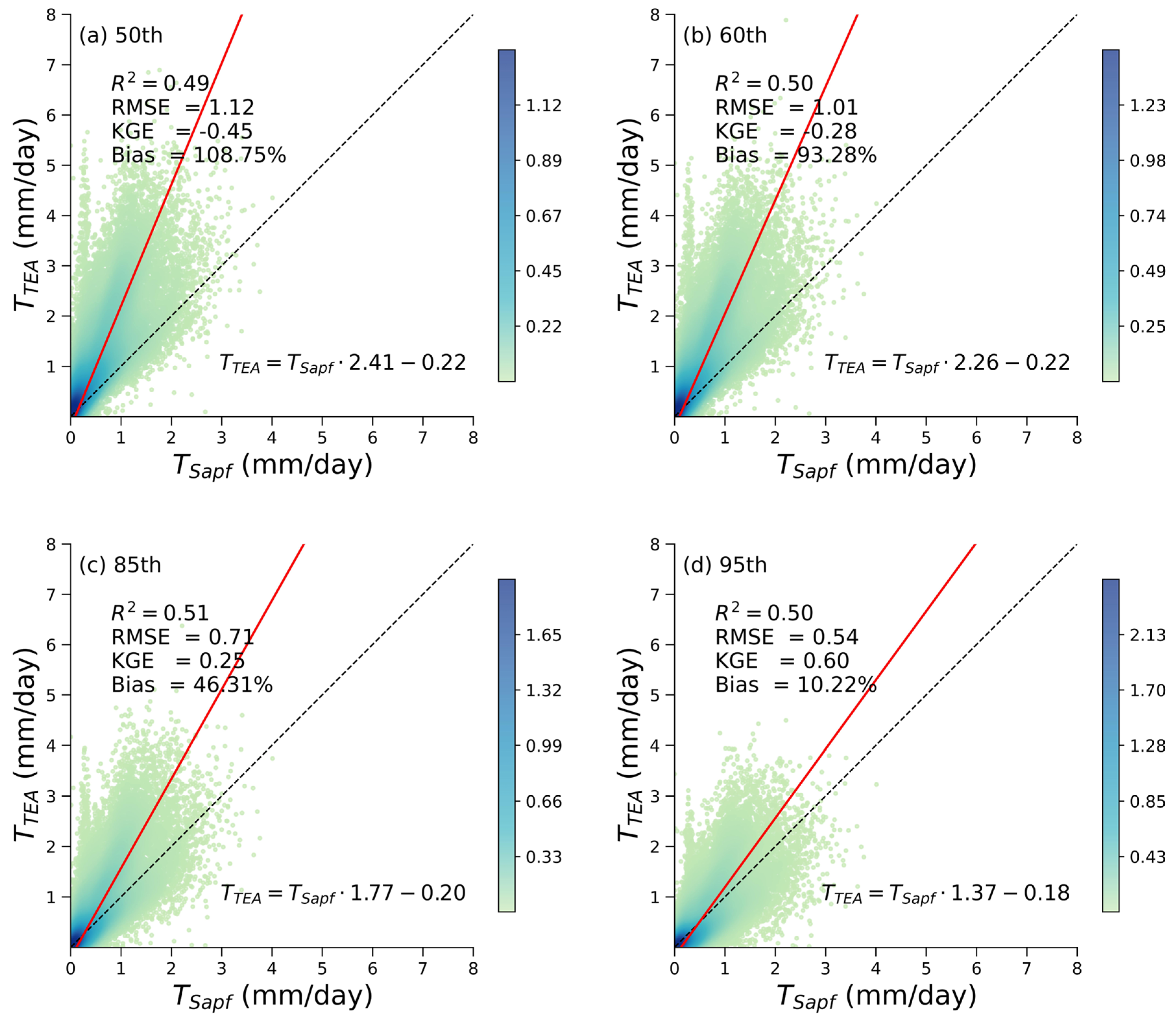
To mitigate the influence of this persistent residual soil evaporation (E_train) in the training dataset, TEA utilizes percentile regression during the prediction phase. In this study, we further compared T estimations using the 50th, 60th, 85th, and 95th percentiles (Figure 15). The 50th percentile led to a substantial overestimation of T (Bias = 104.13%), indicating the pronounced residual soil evaporation in the RF training dataset. In contrast, using the 95th percentile significantly reduced both bias (from 82.78% to 2.47%) and RMSE (to 0.52 mm d⁻¹), increased KGE to 0.65, and maintained a comparable R² value of 0.51. This demonstrates that the initial high error bias was not a structural failure of the TEA algorithm, but rather a parameterization mismatch for ecosystems with high background evaporation. It is particularly noteworthy that the sap flow benchmark dataset used in this validation consists entirely of forest ecosystems (i.e., EBF, ENF, DBF, and MF). Since mature forests typically maintain higher canopy closure and relatively lower persistent soil evaporation compared to wetlands or sparse drylands, the fact that TEA still required the 95th percentile to mitigate an 82.78% bias in these forest sites further underscores the severity of this parameterization issue. As Nelson et al. [28] suggested, sites with high E_train risk severe overestimation. If the default 75th percentile already leads to substantial overestimation in forests, applying it to wetland ecosystems where persistent background evaporation is inherently much higher would likely result in even more extreme biases. Therefore, future research could dynamically adjust the percentile based on site-specific conditions, such as vegetation cover, soil moisture, or water table depth, but this adaptation highly requires ground-truth T data.

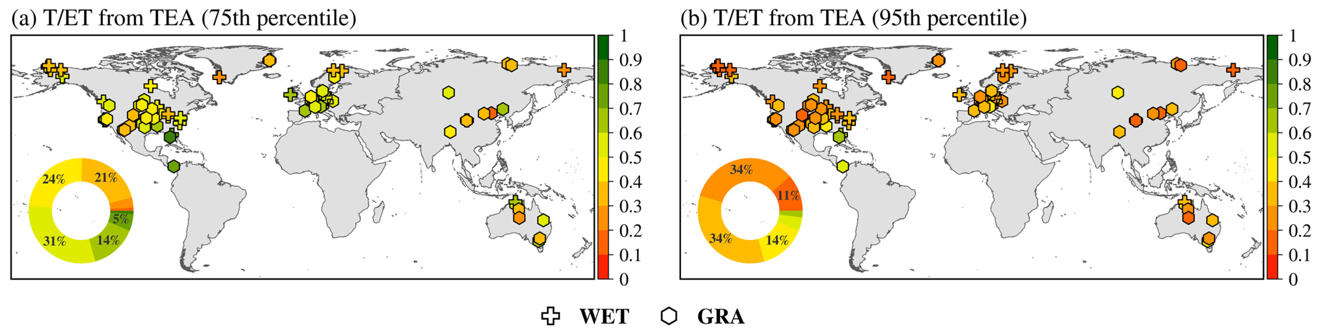
To further explore the necessity of dynamically adjusting the percentiles according to ecosystem types to reduce such positive biases, we evaluated the spatial distribution of TEA-estimated T/ET ratios at 97 globally distributed sites, comprising 62 grassland (GRA) and 35 wetland (WET) ecosystems (Figure 16). When applying the default 75th percentile, TEA yielded high T/ET estimates for these sites, with a mean value of 0.50 for both GRA and WET (Figure 16a). Such a magnitude indicates a systematic positive bias driven by strong background evaporation. However, when the prediction percentile was dynamically adjusted to the 95th, the spatial map exhibited a significant reduction in the magnitude of T/ET across these sites, lowering the mean values to 0.33 for GRA and 0.31 for WET (Figure 16b). This reduction effectively suppressed the overestimation caused by E_train. These spatial distribution results quantitatively confirm that the prediction percentile in the TEA model should not be treated as a static constant. Rather, it is an ecosystem-specific parameter that requires a dynamic shift toward higher percentiles (e.g., ≥95th) in environments with high persistent evaporation to mitigate positive bias.

Among the four ET partitioning methods, Z16 is currently the most widely applied, as it is much simple calculation process and uses widely available half-hourly GPP, ET and VPD as input data without the need for a priori knowledge [52]. However, compared to TEA, Z16 obviously underestimated T (Figure 2 and Figure 4), despite its closer agreement with sap flow data (Figure 5). The underestimation from Z16 is confirmed by many published studies [32,33]. For Z16, uWUE_p is the sole unknown parameter, which needs enough data to estimate [30,33]. Based on the theory of optimal stomatal behavior, uWUE_p is influenced by three key factors, including atmospheric CO₂ concentration (C_a), leaf CO₂ compensation point, and the marginal WUE [27]. Under steady state conditions within a homogenous ecosystem, uWUE_p remains nearly constant. And when soil evaporation is negligible and T is close to ET (T ≈ ET), uWUE_p is approximately equal to the maximum of uWUE_a. The two critical assumptions introduce significant uncertainty into the estimation of uWUE_p. First, soil evaporation cannot be neglected even during peak growing-season periods at some sites, leading to an overestimation of T/ET [53]. Second, multiple vegetation species within a site, changes in C_a and water stress conditions driven by climate variability over the observation period can substantially influence the estimation of uWUE_p. For instance, between 1995 and 2020, C_a rose significantly, which should have led to a corresponding increase in uWUE_p, while a constant uWUEp under such dynamic conditions would likely result in an underestimation of T/ET [33].

Among the four methods, L19 is the most complex. While it does not require prior knowledge of g₁, it relies on many input variables, particularly soil moisture data, which are often unavailable at many EC sites. Figure 2 and Figure 4 revealed L19 had relatively low consistency with the other three methods and slightly overestimates T (Figure 5). Its uncertainty arises from multiple sources. (1) Using the inverted Penman–Monteith equation to calculate G_s. This makes L19 particularly sensitive to data quality and energy closure issues compared to other three methods. When calculating G_s, the estimation of aerodynamic conductance (G_a) increased the complexity. Using USTAR variable to estimate G_a may lead to significant discrepancies of T at annual scale due to data gaps. Alternatively, deriving G_a from a function of wind speed and canopy height requires extensive metadata on measurement height and canopy structure [43], which are often unavailable. Nonetheless, Ref. [32] considered that G_a estimation has limited influence on G_s estimation. (2) L19 assumes that ecosystem surface conductance is the sum of soil and canopy conductances, which implicitly supposes that canopy and soil surface temperatures are equal and it holds under limited conditions. (3) G₀, G₁, and m have fitting errors. L19 uses a non-linear regression model to fit G₀, G₁, and m at six soil moisture bins, and it requires at least 30 data points in each bin. However, the number of valid data points under extremely dry or wet conditions is often insufficient after data filtering, resulting in poor fitting accuracy and reduced reliability in these environments. (4) The structural error introduced by soil moisture data. The use of ERA5-Land reanalysis soil moisture data with 0.1 degree resolution introduces a spatial mismatch with the local EC footprint, which serves as an unquantified structural error. However, because the L19 method utilizes these data primarily for establishing relative percentile bins rather than as absolute physical inputs, the robust temporal dynamics provided by ERA5 help to accurately capture the relative wet–dry cycles, which partially buffers this scale-mismatch uncertainty.

Y21 is the most recently proposed among the four approaches and is unique in requiring prior knowledge of g₁. Similar to Z16, Y21 is simple and feasible to implement at different EC sites and relies on readily available EC observed variables including GPP, ET, VPD, air pressure, and C_a, making it highly suitable for broad application. Validated by the sap flow data (Figure 5), Y21 performed second best only to Z16 and its estimated T values were a little lower than those of TEA but higher than those of Z16. According to [16], the main sources of uncertainty in Y21 arise from three aspects. (1) The parameter g₁ is treated as a constant specific to the ecosystem and vegetation type. (2) The optimality-based unified stomatal conductance model was originally developed for instantaneous timescales, may not represent optimal behavior over longer periods. And (3) the approximation of ecosystem-scale water use efficiency (GPP/T) from leaf-level WUE may not hold consistently across different ecosystems. The last two issues are inherent to the Y21 model; here we focus primarily on the uncertainties associated with the parameter g₁ and missing observation of C_a data at some sites or time periods, both of which can substantially influence T estimates. The parameter g₁ is proven to vary significantly over time. Treating it as a constant fails to capture seasonal adjustments in stomatal strategy. As inferred by Li et al. [32] and Knauer et al. [45], deriving g₁ by fitting it to G_s inverted from the Penman–Monteith equation may be a promising approach.

From a spatial perspective, the applicability of these four methods exhibits distinct divergence when evaluated across water-limited versus energy-limited ecosystems, largely due to their differing sensitivities to physiological and ecological constraints [54]. In water-limited ecosystems (e.g., drylands, savannas, and sparse grasslands), intense radiation and low vegetation cover typically lead to high but highly episodic bare soil evaporation following precipitation. Consequently, the fundamental assumption of T ≈ ET during selected dry periods is severely challenged. As supported by our results, TEA requires strictly elevated prediction percentiles (e.g., 95th) to filter out this persistent residual evaporation [28], while Z16 may underestimate T/ET under dynamic drought stress because its static uWUEp assumption fails to capture rapid stomatal closure and non-linear WUE responses. For L19, while its relative soil moisture binning partially buffers spatial mismatch errors, its non-linear regression relies heavily on the data availability within each bin. In chronically water-limited ecosystems, strict data filtering often leaves an insufficient number of valid data points under extreme soil moisture conditions, resulting in poor fitting accuracy for the empirical conductance parameters (G₀, G₁, and m). Conversely, in energy-limited ecosystems (e.g., high-latitude forests) or environments with continuous water supply (e.g., wetlands), ET is primarily constrained by available radiation. In wetlands, where persistent background evaporation remains exceptionally high, Z16 tends to overestimate T/ET because the underlying assumption that soil evaporation is negligible during peak growth is violated [27]. Moreover, in extremely cold or humid environments, near-zero VPD values can introduce large numerical instabilities in methods heavily dependent on VPD variations, such as Z16 and Y21. Overall, Y21 demonstrates robust applicability across both extremes by dynamically fitting g1 to accommodate different plant hydraulic traits, provided that accurate, high-frequency GPP and VPD data are available [16].

Beyond spatial applicability across diverse ecosystems, the long-term performance of these ET partitioning methods is inherently sensitive to ongoing climate change factors, particularly the rising atmospheric CO₂ concentration (C_a) and increasing VPD. As C_a has risen significantly over the past decades, it has substantially altered plant physiology and enhanced intrinsic WUE by suppressing stomatal conductance without proportionally reducing photosynthesis (i.e., the CO₂ fertilization effect) [45,55], while increasing VPD exacerbates atmospheric evaporative demand, often triggering strict non-linear stomatal closure. Among the four evaluated methods, Y21 theoretically demonstrates the highest resilience to these non-stationary climate drivers. By explicitly incorporating both C_a and VPD into its underlying unified stomatal conductance equations (Equations (16) and (17)), and by dynamically fitting the g₁ parameter on an annual basis, Y21 can effectively trace the long-term physiological adaptations of canopies to climate change [16]. In contrast, while the Z16 method accounts for VPD variations via its square root of VPD formulation, its reliance on a static potential uWUE (uWUE_p) parameter over long observation periods presents a critical limitation. Maintaining a constant uWUE_p under such dynamic conditions with rising actual potential WUE inevitably leads to a progressive underestimation of T/ET [33]. Similarly, the TEA and L19 methods face challenges regarding long-term climatic non-stationarity. Although TEA captures VPD effects implicitly through inputs of air temperature and relative humidity, it completely lacks an explicit C_a input. Consequently, its data-driven random forest model may struggle to accurately extrapolate future WUE trends driven by prolonged CO₂ fertilization if trained on historical periods [16]. For L19, the empirical conductance parameters (G₀, G₁, and m) fitted across soil moisture bins [32,43] may also shift over decades, as elevated C_a and extreme VPD alter the baseline partitioning between canopy and soil conductance. Therefore, integrating explicit C_a parametrization and dynamically tracking physiological responses (e.g., annual g₁ fitting) are highly recommended for future ET partitioning models to maintain accuracy under changing climate scenarios.

4.2. Uncertainties in Sap Flow-Based Transpiration Estimates

Sap flow measurements serve as a critical independent benchmark for validating ET partitioning methods in this study. However, they contain inherent uncertainties when upscaled from individual trees to the ecosystem level. These uncertainties mainly stem from the exclusion of understory vegetation, spatial scaling biases, and sensor-specific limitations.

First, the sap flow-based stand transpiration (T_sapf) likely represents a lower bound of the total ecosystem transpiration, inherently creating an observation gap when compared to EC-driven models. As detailed by Poyatos et al. [18] in a global synthesis of the SAPFLUXNET database, sap flow sensors are typically installed on dominant canopy trees, which frequently excludes smaller-diameter stems and the shrub or herbaceous layers. However, the ET partitioning methods evaluated in this study are driven by EC measurements, which inherently integrate the water and carbon fluxes of the entire ecosystem footprint encompassing both the overstory and the understory [14]. Consequently, the systematic positive biases observed across all four methods (e.g., 33.22% to 82.78%) do not solely indicate model overestimations, but partially represent a structural observation mismatch. For instance, Rafi et al. [12] demonstrated that sap flow measurements significantly underestimated total transpiration compared to lysimeters precisely because they missed the flux from lower canopy layers. This footprint discrepancy explains why the baseline T_sapf appears systematically lower, and why conservative estimates like Z16 align best with the overstory-restricted sap flow dynamics.

Second, while the upscaling process from individual trees to the stand footprint inherently introduces spatial uncertainties, the detailed biometric parameters (stand basal area and stand density) listed in Table 1 were specifically utilized to mitigate these representativeness biases. Rather than adopting a simple multiplication of average tree sap flow by total tree count which overlooks tree size variations and stand heterogeneity, we implemented a species-specific, basal-area-weighted upscaling approach [19]. By normalizing plant-level sap flow by its basal area and subsequently scaling it using the total basal area occupied by that species, the disproportionate contributions of different tree sizes and species were explicitly accounted for. Furthermore, rescaling the total sap flow to encompass the basal area of unmeasured species (as described in Section 2.1.3) effectively buffered the bias caused by limited sensor sample sizes within mixed stands. This rigorous integration of stand density and basal area minimized the structural mismatch between the sampled trees and the actual EC footprint, yielding a more robust and representative ecosystem scale T_sapf benchmark.

Finally, systematic errors associated with the thermal dissipation probes (TDPs) contribute to an underestimation of T. According to Poyatos et al. [18], the TDP method (Granier) is the most widely used technique in the SAPFLUXNET database. Recent evaluations by Dix and Aubrey [56] revealed that standard TDP sensors tend to underestimate sap flux density by up to 50% if used without species-specific calibration. This error arises from radial variation and thermal gradients. Species-specific calibration was not universally applied across the historical datasets used in this study [56]. Therefore, the resulting T_sapf is likely conservative. This systematic instrument bias further explains our results: the Z16 method yields the lowest T estimates, yet it showed the highest agreement with the sap flow benchmark.

5. Conclusions

This study systematically evaluated four ET partitioning methods (i.e., TEA, Z16, L19, and Y21) across 368 global eddy covariance sites and 15 sap flow sites. Intercomparison results for the four ET partitioning methods at daily and annual scales showed that TEA and Y21, Z16 and Y21 produced higher consistency, whereas L19 had lower consistency with other methods. Regarding the magnitude of T values, TEA > Y21 > L19 > Z16. Validation against sap flow data indicated that all four methods captured the temporal dynamics of T reasonably well (R² = 0.44–0.47). Among them, Z16 performed best (R² = 0.45, KGE = 0.52), followed by Y21, while TEA showed the lowest accuracy due to systematic overestimation. Analysis of annual T and T/ET across 201 sites revealed that the global mean annual T ranged from 213 mm yr⁻¹ (Z16) to 294 mm yr⁻¹ (TEA), and annual T/ET varied between 0.45 (Z16) and 0.63 (TEA). Trend analysis at 91 sites further indicated increasing trends in both annual T (0.33–0.83 mm yr⁻²) and annual T/ET (0.0015–0.0019 yr⁻¹) across all methods, despite divergence among ecosystem types. Particularly in cropland ecosystems, this detected increasing trend in T/ET holds critical implications for sustainable agricultural water management. A rising T/ET ratio indicates that a greater proportion of consumptive water use is partitioned into productive crop transpiration rather than non-productive soil evaporation, which fundamentally alters the calculation of irrigation efficiency. Consequently, agricultural water models must account for this shift to avoid overestimating crop water requirements or inaccurately projecting the return flows available for aquifer recharge. Additional correlation analysis demonstrated that the relationship between GPP and T was consistently stronger than that between GPP and ET, suggesting that all four methods effectively represent the coupled carbon–water relationship at the ecosystem scale. Although the four methods differ substantially in model assumptions, structure, and parameterization, leading to uncertainties in absolute T estimates, they all captured the temporal dynamics of T satisfactorily. We therefore recommend applying multiple ET partitioning approaches when comparing annual T or T/ET values to reduce estimation uncertainty. Incorporating these dynamic ET partitioning evaluations into agrometeorological assessments will be essential for advancing precision irrigation and ensuring groundwater sustainability, thereby contributing directly to global Sustainable Development Goals.

References

1. Xiao, W.; Wei, Z.; Wen, X. Evapotranspiration Partitioning at the Ecosystem Scale Using the Stable Isotope Method—A Review. Agric. For. Meteorol. 2018, 263, 346–361. [Google Scholar] [CrossRef]
2. Jasechko, S.; Sharp, Z.D.; Gibson, J.J.; Birks, S.J.; Yi, Y.; Fawcett, P.J. Terrestrial Water Fluxes Dominated by Transpiration. Nature 2013, 496, 347–350. [Google Scholar] [CrossRef]
3. Bai, Y.; Mallick, K.; Hu, T.; Zhang, S.; Yang, S.; Ahmadi, A. Integrating Machine Learning with Thermal-Driven Analytical Energy Balance Model Improved Terrestrial Evapotranspiration Estimation through Enhanced Surface Conductance. Remote Sens. Environ. 2024, 311, 114308. [Google Scholar] [CrossRef]
4. Fu, J.; Wang, W.; Shao, Q.; Xing, W.; Cao, M.; Wei, J.; Chen, Z.; Nie, W. Improved Global Evapotranspiration Estimates Using Proportionality Hypothesis-Based Water Balance Constraints. Remote Sens. Environ. 2022, 279, 113140. [Google Scholar] [CrossRef]
5. He, M.; Kimball, J.S.; Yi, Y.; Running, S.W.; Guan, K.; Moreno, A.; Wu, X.; Maneta, M. Satellite Data-Driven Modeling of Field Scale Evapotranspiration in Croplands Using the MOD16 Algorithm Framework. Remote Sens. Environ. 2019, 230, 111201. [Google Scholar] [CrossRef]
6. Kan, Y.; Shao, H.; Yao, Y.; Li, Y.; Zhang, X.; Xu, J.; Zhang, X.; Xie, Z.; Ning, J.; Yu, R.; et al. Evaluation of Two Strategies from the SEBS Model for Estimating the Daily Terrestrial Evapotranspiration Values of the Tibetan Plateau. J. Hydrol. 2025, 656, 132921. [Google Scholar] [CrossRef]
7. Koppa, A.; Rains, D.; Hulsman, P.; Poyatos, R.; Miralles, D.G. A Deep Learning-Based Hybrid Model of Global Terrestrial Evaporation. Nat. Commun. 2022, 13, 1912. [Google Scholar] [CrossRef] [PubMed]
8. Li, C.; Han, J.; He, Y.; Shen, J.; Liu, Z.; Yang, H. Assessing Global Transpiration Estimates: Insights from Tree-Scale Sap Flow Analysis. J. Hydrol. 2024, 637, 131419. [Google Scholar] [CrossRef]
9. Niu, Z.; He, H.; Zhu, G.; Ren, X.; Zhang, L.; Zhang, K.; Yu, G.; Ge, R.; Li, P.; Zeng, N.; et al. An Increasing Trend in the Ratio of Transpiration to Total Terrestrial Evapotranspiration in China from 1982 to 2015 Caused by Greening and Warming. Agric. For. Meteorol. 2019, 279, 107701. [Google Scholar] [CrossRef]
10. Jiang, F.; Xie, X.; Wang, Y.; Liang, S.; Zhu, B.; Meng, S.; Zhang, X.; Chen, Y.; Liu, Y. Vegetation Greening Intensified Transpiration but Constrained Soil Evaporation on the Loess Plateau. J. Hydrol. 2022, 614, 128514. [Google Scholar] [CrossRef]
11. Wehr, R.; Commane, R.; Munger, J.W.; Barry Mcmanus, J.; Nelson, D.D.; Zahniser, M.S.; Saleska, S.R.; Wofsy, S.C. Dynamics of Canopy Stomatal Conductance, Transpiration, and Evaporation in a Temperate Deciduous Forest, Validated by Carbonyl Sulfide Uptake. Biogeosciences 2017, 14, 389–401. [Google Scholar] [CrossRef]
12. Rafi, Z.; Merlin, O.; Le Dantec, V.; Khabba, S.; Mordelet, P.; Er-Raki, S.; Amazirh, A.; Olivera-Guerra, L.; Ait Hssaine, B.; Simonneaux, V.; et al. Partitioning Evapotranspiration of a Drip-Irrigated Wheat Crop: Inter-Comparing Eddy Covariance-, Sap Flow-, Lysimeter- and FAO-Based Methods. Agric. For. Meteorol. 2019, 265, 310–326. [Google Scholar] [CrossRef]
13. Rothfuss, Y.; Quade, M.; Brüggemann, N.; Graf, A.; Vereecken, H.; Dubbert, M. Reviews and Syntheses: Gaining Insights into Evapotranspiration Partitioning with Novel Isotopic Monitoring Methods. Biogeosciences 2021, 18, 3701–3732. [Google Scholar] [CrossRef]
14. Wang, H.; Li, X.; Xiao, J.; Ma, M. Evapotranspiration Components and Water Use Efficiency from Desert to Alpine Ecosystems in Drylands. Agric. For. Meteorol. 2021, 298–299, 108283. [Google Scholar] [CrossRef]
15. Yuan, Y.; Wang, L.; Wang, H.; Lin, W.; Jiao, W.; Du, T. A Modified Isotope-Based Method for Potential High-Frequency Evapotranspiration Partitioning. Adv. Water Resour. 2022, 160, 104103. [Google Scholar] [CrossRef]
16. Yu, L.; Zhou, S.; Zhao, X.; Gao, X.; Jiang, K.; Zhang, B.; Cheng, L.; Song, X.; Siddique, K.H.M. Evapotranspiration Partitioning Based on Leaf and Ecosystem Water Use Efficiency. Water Resour. Res. 2022, 58, e2021WR030629. [Google Scholar] [CrossRef]
17. Wang, J.; Renninger, H.J. SapFlower: An Automated Tool for Sap Flow Data Preprocessing, Gap-Filling, and Analysis Using Deep Learning. New Phytol. 2025, 246, 2324–2345. [Google Scholar] [CrossRef] [PubMed]
18. Poyatos, R.; Granda, V.; Flo, V.; Adams, M.A.; Adorján, B.; Aguadé, D.; Aidar, M.P.M.; Allen, S.; Alvarado-Barrientos, M.S.; Anderson-Teixeira, K.J.; et al. Global Transpiration Data from Sap Flow Measurements: The SAPFLUXNET Database. Earth Syst. Sci. Data 2021, 13, 2607–2649. [Google Scholar] [CrossRef]
19. Bright, R.M.; Miralles, D.G.; Poyatos, R.; Eisner, S. Simple Models Outperform More Complex Big-Leaf Models of Daily Transpiration in Forested Biomes. Geophys. Res. Lett. 2022, 49, e2022GL100100. [Google Scholar] [CrossRef]
20. Schlesinger, W.H.; Jasechko, S. Transpiration in the Global Water Cycle. Agric. For. Meteorol. 2014, 189–190, 115–117. [Google Scholar] [CrossRef]
21. Wang, X.; Li, Z.; Zhou, Y.; Wang, Y.; Ahmad, S.; Hu, M.; Sun, S.; Huang, H.; Zhang, J.; Zhai, L. Evaluation of Water Use Efficiency Model in Evapotranspiration Partitioning from High-Frequency Eddy Covariance Data—A Comparison between Plantation Sites. Agric. For. Meteorol. 2025, 372, 110663. [Google Scholar] [CrossRef]
22. Pastorello, G.; Trotta, C.; Canfora, E.; Chu, H.; Christianson, D.; Cheah, Y.W.; Poindexter, C.; Chen, J.; Elbashandy, A.; Humphrey, M.; et al. The FLUXNET2015 Dataset and the ONEFlux Processing Pipeline for Eddy Covariance Data. Sci. Data 2020, 7, 225. [Google Scholar] [CrossRef]
23. Lu, L.; Zhang, D.; Zhang, J.; Zhang, J.; Zhang, S.; Bai, Y.; Yang, S. Ecosystem Evapotranspiration Partitioning and Its Spatial–Temporal Variation Based on Eddy Covariance Observation and Machine Learning Method. Remote Sens. 2023, 15, 4831. [Google Scholar] [CrossRef]
24. Zhang, J.; Yang, S.; Wang, J.; Zeng, R.; Zhang, S.; Bai, Y.; Zhang, J. Evapotranspiration Partitioning for Croplands Based on Eddy Covariance Measurements and Machine Learning Models. Agronomy 2025, 15, 512. [Google Scholar] [CrossRef]
25. Scanlon, T.M.; Sahu, P. On the Correlation Structure of Water Vapor and Carbon Dioxide in the Atmospheric Surface Layer: A Basis for Flux Partitioning. Water Resour. Res. 2008, 44, W10418. [Google Scholar] [CrossRef]
26. Scanlon, T.M.; Kustas, W.P. Partitioning Carbon Dioxide and Water Vapor Fluxes Using Correlation Analysis. Agric. For. Meteorol. 2010, 150, 89–99. [Google Scholar] [CrossRef]
27. Zhou, S.; Yu, B.; Zhang, Y.; Huang, Y.; Wang, G. Partitioning Evapotranspiration Based on the Concept of Underlying Water Use Efficiency. Water Resour. Res. 2016, 52, 1160–1175. [Google Scholar] [CrossRef]
28. Nelson, J.A.; Carvalhais, N.; Cuntz, M.; Delpierre, N.; Knauer, J.; Ogée, J.; Migliavacca, M.; Reichstein, M.; Jung, M. Coupling Water and Carbon Fluxes to Constrain Estimates of Transpiration: The TEA Algorithm. J. Geophys. Res. Biogeosci. 2018, 123, 3617–3632. [Google Scholar] [CrossRef]
29. Scott, R.L.; Knowles, J.F.; Nelson, J.A.; Gentine, P.; Li, X.; Barron-Gafford, G.; Bryant, R.; Biederman, J.A. Water Availability Impacts on Evapotranspiration Partitioning. Agric. For. Meteorol. 2021, 297, 108251. [Google Scholar] [CrossRef]
30. Yang, S.; Zhang, J.; Han, J.; Bai, Y.; Xun, L.; Zhang, S.; Cao, D.; Wang, J. The Ratio of Transpiration to Evapotranspiration Dominates Ecosystem Water Use Efficiency Response to Drought. Agric. For. Meteorol. 2025, 363, 110423. [Google Scholar] [CrossRef]
31. Medlyn, B.E.; Duursma, R.A.; Eamus, D.; Ellsworth, D.S.; Prentice, I.C.; Barton, C.V.M.; Crous, K.Y.; De Angelis, P.; Freeman, M.; Wingate, L. Reconciling the Optimal and Empirical Approaches to Modelling Stomatal Conductance. Glob. Change Biol. 2011, 17, 2134–2144. [Google Scholar] [CrossRef]
32. Li, X.; Gentine, P.; Lin, C.; Zhou, S.; Sun, Z.; Zheng, Y.; Liu, J.; Zheng, C. A Simple and Objective Method to Partition Evapotranspiration into Transpiration and Evaporation at Eddy-Covariance Sites. Agric. For. Meteorol. 2019, 265, 171–182. [Google Scholar] [CrossRef]
33. Hu, X.; Lei, H. Evapotranspiration Partitioning and Its Interannual Variability over a Winter Wheat-Summer Maize Rotation System in the North China Plain. Agric. For. Meteorol. 2021, 310, 108635. [Google Scholar] [CrossRef]
34. Eichelmann, E.; Mantoani, M.C.; Chamberlain, S.D.; Hemes, K.S.; Oikawa, P.Y.; Szutu, D.; Valach, A.; Verfaillie, J.; Baldocchi, D.D. A Novel Approach to Partitioning Evapotranspiration into Evaporation and Transpiration in Flooded Ecosystems. Glob. Change Biol. 2022, 28, 990–1007. [Google Scholar] [CrossRef]
35. Perez-Priego, O.; Katul, G.; Reichstein, M.; El-Madany, T.S.; Ahrens, B.; Carrara, A.; Scanlon, T.M.; Migliavacca, M. Partitioning Eddy Covariance Water Flux Components Using Physiological and Micrometeorological Approaches. J. Geophys. Res. Biogeosci. 2018, 123, 3353–3370. [Google Scholar] [CrossRef]
36. Rigden, A.J.; Salvucci, G.D.; Entekhabi, D.; Short Gianotti, D.J. Partitioning Evapotranspiration Over the Continental United States Using Weather Station Data. Geophys. Res. Lett. 2018, 45, 9605–9613. [Google Scholar] [CrossRef]
37. Stoy, P.C.; El-Madany, T.S.; Fisher, J.B.; Gentine, P.; Gerken, T.; Good, S.P.; Klosterhalfen, A.; Liu, S.; Miralles, D.G.; Perez-Priego, O.; et al. Reviews and Syntheses: Turning the Challenges of Partitioning Ecosystem Evaporation and Transpiration into Opportunities. Biogeosciences 2019, 16, 3747–3775. [Google Scholar] [CrossRef]
38. Nelson, J.A.; Pérez-Priego, O.; Zhou, S.; Poyatos, R.; Zhang, Y.; Blanken, P.D.; Gimeno, T.E.; Wohlfahrt, G.; Desai, A.R.; Gioli, B.; et al. Ecosystem Transpiration and Evaporation: Insights from Three Water Flux Partitioning Methods across FLUXNET Sites. Glob. Change Biol. 2020, 26, 6916–6930. [Google Scholar] [CrossRef]
39. ICOS Ecosystem Thematic Centre Warm Winter 2020 Ecosystem Eddy Covariance Flux Product for 73 Stations in FLUXNET-Archive Format. Available online: https://www.icos-cp.eu/data-products/2G60-ZHAK (accessed on 14 December 2025).
40. Novick, K.A.; Biederman, J.A.; Desai, A.R.; Litvak, M.E.; Moore, D.J.P.; Scott, R.L.; Torn, M.S. The AmeriFlux Network: A Coalition of the Willing. Agric. For. Meteorol. 2018, 249, 444–456. [Google Scholar] [CrossRef]
41. Muñoz-Sabater, J.; Dutra, E.; Agustí-Panareda, A.; Albergel, C.; Arduini, G.; Balsamo, G.; Boussetta, S.; Choulga, M.; Harrigan, S.; Hersbach, H.; et al. ERA5-Land: A State-of-the-Art Global Reanalysis Dataset for Land Applications. Earth Syst. Sci. Data 2021, 13, 4349–4383. [Google Scholar] [CrossRef]
42. Gorelick, N.; Hancher, M.; Dixon, M.; Ilyushchenko, S.; Thau, D.; Moore, R. Google Earth Engine: Planetary-Scale Geospatial Analysis for Everyone. Remote Sens. Environ. 2017, 202, 18–27. [Google Scholar] [CrossRef]
43. Lin, C.; Gentine, P.; Huang, Y.; Guan, K.; Kimm, H.; Zhou, S. Diel Ecosystem Conductance Response to Vapor Pressure Deficit Is Suboptimal and Independent of Soil Moisture. Agric. For. Meteorol. 2018, 250–251, 24–34. [Google Scholar] [CrossRef]
44. Beer, C.; Ciais, P.; Reichstein, M.; Baldocchi, D.; Law, B.E.; Papale, D.; Soussana, J.-F.; Ammann, C.; Buchmann, N.; Frank, D.; et al. Temporal and Among-site Variability of Inherent Water Use Efficiency at the Ecosystem Level. Global Biogeochem. Cycles 2009, 23, GB2018. [Google Scholar] [CrossRef]
45. Knauer, J.; Zaehle, S.; Medlyn, B.E.; Reichstein, M.; Williams, C.A.; Migliavacca, M.; De Kauwe, M.G.; Werner, C.; Keitel, C.; Kolari, P.; et al. Towards Physiologically Meaningful Water-use Efficiency Estimates from Eddy Covariance Data. Glob. Change Biol. 2018, 24, 694–710. [Google Scholar] [CrossRef]
46. Gupta, H.V.; Kling, H.; Yilmaz, K.K.; Martinez, G.F. Decomposition of the Mean Squared Error and NSE Performance Criteria: Implications for Improving Hydrological Modelling. J. Hydrol. 2009, 377, 80–91. [Google Scholar] [CrossRef]
47. Knoben, W.J.M.; Freer, J.E.; Woods, R.A. Technical Note: Inherent Benchmark or Not? Comparing Nash–Sutcliffe and Kling–Gupta Efficiency Scores. Hydrol. Earth Syst. Sci. 2019, 23, 4323–4331. [Google Scholar] [CrossRef]
48. Taylor, K.E. Summarizing Multiple Aspects of Model Performance in a Single Diagram. J. Geophys. Res. Atmos. 2001, 106, 7183–7192. [Google Scholar] [CrossRef]
49. Jefferson, T. Proceedings of the 40th Conference on Winter Simulation; Winter Simulation Conference: Washington, DC, USA, 2008; ISBN 9781424427086. [Google Scholar]
50. Zhao, W.; Rong, Y.; Zhou, Y.; Zhang, Y.; Li, S.; Liu, L. The Relationship of Gross Primary Productivity with NDVI Rather than Solar-Induced Chlorophyll Fluorescence Is Weakened under the Stress of Drought. Remote Sens. 2024, 16, 555. [Google Scholar] [CrossRef]
51. Tang, J.; Peng, X.; Peng, W. Nonlinear Variations and Drivers of Vegetation NPP on the Tibetan Plateau: Interaction of Natural and Human Factors. PLoS ONE 2025, 20, e0320370. [Google Scholar] [CrossRef]
52. Chen, Y.; Ding, Z.; Yu, P.; Yang, H.; Song, L.; Fan, L.; Han, X.; Ma, M.; Tang, X. Quantifying the Variability in Water Use Efficiency from the Canopy to Ecosystem Scale across Main Croplands. Agric. Water Manag. 2022, 262, 107427. [Google Scholar] [CrossRef]
53. Bai, Y.; Li, X.; Zhou, S.; Yang, X.; Yu, K.; Wang, M.; Liu, S.; Wang, P.; Wu, X.; Wang, X.; et al. Quantifying Plant Transpiration and Canopy Conductance Using Eddy Flux Data: An Underlying Water Use Efficiency Method. Agric. For. Meteorol. 2019, 271, 375–384. [Google Scholar] [CrossRef]
54. Cao, R.; Huang, H.; Wu, G.; Han, D.; Jiang, Z.; Di, K.; Hu, Z. Spatiotemporal Variations in the Ratio of Transpiration to Evapotranspiration and Its Controlling Factors across Terrestrial Biomes. Agric. For. Meteorol. 2022, 321, 108984. [Google Scholar] [CrossRef]
55. Keenan, T.F.; Hollinger, D.Y.; Bohrer, G.; Dragoni, D.; Munger, J.W.; Schmid, H.P.; Richardson, A.D. Increase in Forest Water-Use Efficiency as Atmospheric Carbon Dioxide Concentrations Rise. Nature 2013, 499, 324–327. [Google Scholar] [CrossRef] [PubMed]
56. Dix, M.J.; Aubrey, D.P. Calibration Approach and Range of Observed Sap Flow Influences Transpiration Estimates from Thermal Dissipation Sensors. Agric. For. Meteorol. 2021, 307, 108534. [Google Scholar] [CrossRef]
Figure 1. (a) Spatial distribution of the 368 eddy-covariance sites used in this study. (b,c) Details of the black boxes in (a). The 12 IGBP ecosystem types include: evergreen needleleaf forests (ENF), evergreen broadleaf forests (EBF), deciduous broadleaf forests (DBF), deciduous needleleaf forests (DNF), mixed forests (MF), croplands (CRO), grasslands (GRA), savannas (SAV), woody savannas (WSA), open shrublands (OSH), closed shrublands (CSH), and permanent wetlands (WET). The number of sites for each type is indicated in the text.
Sustainability 18 03245 g001
Figure 2. Comparison of daily transpiration (T) estimates from the four ET partitioning methods: (a) TEA vs. Z16; (b) L19 vs. Z16; (c) Y21 vs. Z16; (d) TEA vs. L19; (e) Y21 vs. L19; and (f) Y21 vs. TEA. The solid red line represents the fitted line, and the dashed black line indicates the 1:1 line.
Sustainability 18 03245 g002
Figure 3. Comparison of daily (a,c,e,g) and annual T (b,d,f,h) estimates from the four ET partitioning methods (TTEA, TZ16, TL19, and TY21) across the 12 ecosystem types.
Sustainability 18 03245 g003
Figure 4. Comparison of annual T estimates from the four ET partitioning methods: (a) TEA vs. Z16; (b) L19 vs. Z16; (c) Y21 vs. Z16; (d) TEA vs. L19; (e) Y21 vs. L19; and (f) Y21 vs. TEA. The solid red line represents the fitted line, and the dashed black line indicates the 1:1 line.
Sustainability 18 03245 g004
Figure 5. Validation of daily T derived from the four ET partitioning methods against the sap flow data: (a) TEA; (b) Z16; (c) L19; and (d) Y21. The solid red line represents the fitted line, and the dashed black line indicates the 1:1 line.
Sustainability 18 03245 g005
Figure 6. Taylor diagram for the validation of daily T from the four ET partitioning methods against the sap flow data.
Sustainability 18 03245 g006
Figure 7. Validation of daily T from the four ET partitioning methods using the sap flow data at 15 SAP-FLUXNET sites.
Sustainability 18 03245 g007
Figure 8. The temporal dynamics of daily T from the four ET partitioning methods, ET, and T from sap flow data (Tsapf) at six sap flow sites, i.e., (a) AU-Cum (EBF), (b) FR-Fon (DBF), (c) FR-Pue (EBF), (d) NL-Loo (ENF), (e) RU-Fyo (ENF), and (f) US-UMB (DBF).
Sustainability 18 03245 g008
Figure 9. Spatial distributions of multi-year mean T and T/ET estimated by the four methods (TEA, Z16, L19, and Y21). The ring charts show the percentage of sites within each interval.
Sustainability 18 03245 g009
Figure 10. The boxplot of annual T and T/ET from the four methods (TEA, Z16, L19, and Y21) across different ecosystem types. In the boxplots, the black dots represent the mean values, and the solid lines represent the medians. The horizontal dashed lines indicate the mean value for each method, and “n” denotes the number of valid sites.
Sustainability 18 03245 g010
Figure 11. The boxplot of annual T and T/ET from the four methods (TEA, Z16, L19, and Y21) across the five primary Köppen–Geiger climate zones. In the boxplots, the black dots represent the mean values, and the solid lines represent the medians. The horizontal dashed lines indicate the mean value for each method, and “n” denotes the number of valid sites.
Sustainability 18 03245 g011
Figure 12. Spatial distributions of interannual trends in annual T and T/ET estimated by four methods (TEA, Z16, L19, and Y21) at 91 sites. The ring charts show the percentage of sites within each category.
Sustainability 18 03245 g012
Figure 13. Spatial distribution of the Pearson correlation coefficients (r) between annual GPP and (a) TTEA, (b) TZ16, (c) TL19, (d) TY21, and (e) ET across 91 sites.
Sustainability 18 03245 g013
Figure 14. Validation of daily T derived from the TEA method with four different CSWI thresholds: (a) 1 mm, (b) 0 mm, (c) −1 mm, and (d) −1.5 mm against the sap flow data. The solid red line represents the fitted line, and the dashed black line indicates the 1:1 line.
Sustainability 18 03245 g014
Figure 15. Validation of daily T derived from the TEA method with four different quantiles: (a) 50th, (b) 60th, (c) 85th, and (d) 95th against the sap flow data. The solid red line represents the fitted line, and the dashed black line indicates the 1:1 line.
Sustainability 18 03245 g015
Figure 16. Spatial distributions of multi-year mean T/ET estimated by the TEA method using the (a) 75th and (b) 95th percentiles across 97 sites (62 grassland and 35 wetland ecosystems). The ring charts show the percentage of sites within each interval.
Sustainability 18 03245 g016