Digital Economy, Green Innovation, and Agricultural Carbon Emission Reduction: Spillover Effects and Analyses of Mechanisms
Abstract
1. Introduction
2. Literature Review
2.1. The “Double-Edged Sword” Effect and Comprehensive Impact of the Digital Economy on Carbon Emissions
2.2. The Digital Economy and Agricultural Carbon Emissions: An Emerging Research Focus
2.3. Research Gaps and Major Contributions of This Study
- (1).
- The mechanism’s black box needs to be opened. Most existing studies directed at examining the relationships among the digital economy, green innovation, and agricultural carbon emissions have done so in isolated frameworks or merely provide theoretical descriptions. Accordingly, they lack an empirical testing of the complete transmission path of “digital economy → green innovation → agricultural carbon reduction,” leaving the intrinsic mechanisms involved confined in a “black box.”
- (2).
- The spatial perspective remains underdeveloped. Although some studies have noted spatial spillover effects, they are often limited to a single spatial weight matrix (e.g., geographic contiguity). In this way, there is a lack of any robust comparative analysis of spillover effects under different spatial weight matrices (e.g., geographical/economic distances) that can result from multi-dimensional perspectives such as technology diffusion and market integration.
- (3).
- Nonlinear relationships remain underexplored. The complexity of agricultural systems indicates that the emission reduction effect of the digital economy may be constrained by the external environment. The existing literature generally ignores the threshold effects of key macro variables such as the urbanization rates. As a result, it fails to reveal the boundary conditions under which the digital economy’s emission reduction effect operates.
- (1).
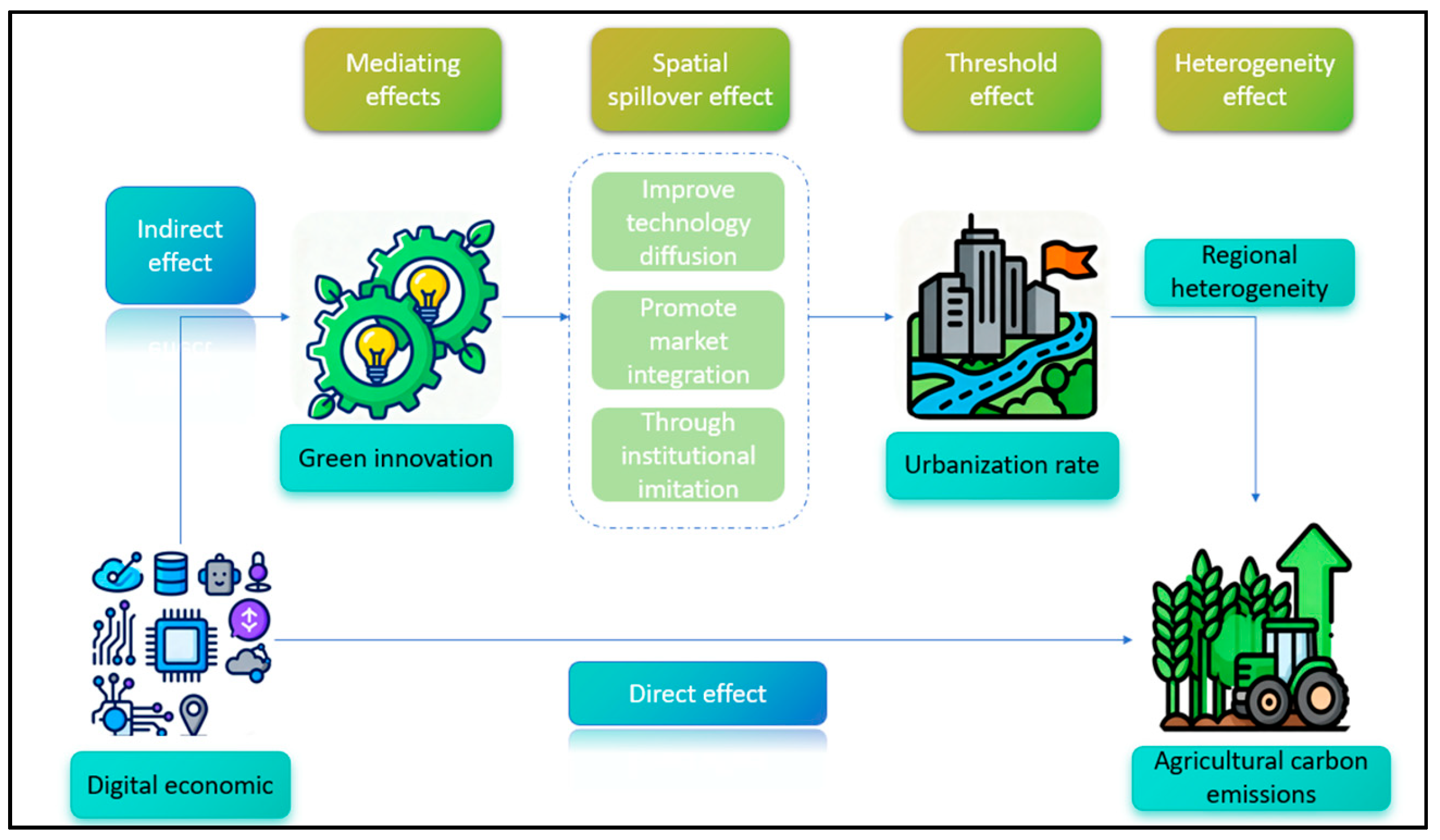
- Integrated Theoretical Framework: Construction of an integrated analytical framework of “digital economy—green innovation—agricultural carbon emissions,” and the first-time use of a mediation effects model to empirically test the core mediating role of green innovation.
- (2).
- Methodological Cross-Innovation: By innovatively combining the Spatial Durbin Model (SDM) with the panel threshold model, we not only quantify the robustness of spatial spillover effects but also reveal the nonlinear moderating role of urbanization rates on the core relationship.
- (3).
- Targeted Policy Implications: With use of heterogeneity analysis and threshold effect identification, differentiated and actionable policy insights for regions with different developmental stages and regional specific characteristics were achieved. In this way, the “one-size-fits-all” policy trap can be avoided.
3. Research Hypotheses and Theoretical Framework
3.1. Direct Effect of the Digital Economy on Agricultural Carbon Emissions
3.2. The Impact of Green Innovation on Agricultural Carbon Emissions
3.2.1. Direct Emission Reduction Effects
3.2.2. Indirect Emission Reduction Effects
3.3. Spatial Spillover Effects of the Digital Economy on Agricultural Carbon Emissions
3.4. Threshold Effect of Urbanization on the Digital Economy’s Impact on Agricultural Carbon Emissions
4. Research Design
4.1. Econometric Model Design
4.1.1. Linear Regression Model
4.1.2. Mediation Effect Model
4.1.3. Spatial Panel Model
- (1).
- Contiguity Matrix (W1):
- (2).
- Geographic Distance Matrix (W2):
4.1.4. Threshold Effect
4.2. Variable Selection
4.2.1. Dependent Variable: Agricultural Carbon Emissions (ACE)
4.2.2. Core Explanatory Variable: Digital Economy Index (DE)
4.2.3. Mediating Variable: Green Innovation (GI)
4.2.4. Control Variables (Z)
- (1).
- Rural Population Size (Rps): Measured by the number of rural residents [53], Rps reflects the rural population scale [19]. While this variable may include non-agricultural rural residents, it remains a valid reflection of the overall rural demographic context that influences agricultural land use, energy consumption, and production structure.
- (2).
- Rural Electricity Consumption (Rec): An indicator of rural economic development, resident quality of life, and agricultural modernization level, reflecting the intensity of production activities and household electrification.
- (3).
- Urbanization Rate (Ur): Measured as the proportion of urban population to total population, Ur reflects changes in urban–rural population structure [54].
- (4).
- Proportion of Fiscal Expenditure on Agriculture (Fsa): Reflects government investment in agriculture, potentially influencing the adoption of green technologies and infrastructure upgrades [55].
- (5).
- Share of Agricultural Added Value (Aav): Measured as the proportion of primary industry (agriculture) added value to GDP, Aav indicates the importance of agriculture in the regional economic structure.
4.3. Data Sources and Descriptive Statistics
5. Empirical Analysis
5.1. Impact Analysis of the Digital Economy on Agricultural Carbon Emissions
- (1)
- Is the overall inhibitory effect of DE on ACE robust (Table 4)?
- (2)
- How does the direction of control variable effects reveal structural contradictions in agricultural carbon emissions?
- (3)
- How can reliability be ensured through multi-dimensional robustness tests (replacing variable measurement methods and sub-period regression)?
5.1.1. Benchmark Regression Analysis
5.1.2. Robustness Checks
- (1)
- Instrumental variable (IV) method
- (2)
- Sensitivity Tests for Missing Value Processing
- (1).
- No Imputation, Balanced Panel: All observations with missing values were removed, resulting in a balanced panel dataset containing 298 observations.
- (2).
- Multiple Imputation (MICE): Multiple imputations were performed using the Multiple Imputation by Chained Equations (MICE) method. With this procedure, 2 imputed datasets were generated.

| No Imputation: Balanced Panel Regression | Multiple Imputation (MICE) | |
|---|---|---|
| Variables | LnACE | LnACE |
| DE | −1.995 *** | −2.053 *** |
| (−3.92) | (−4.00) | |
| Rps | 0.001 *** | 0.001 *** |
| (14.13) | (14.81) | |
| Rec | 0.000 *** | 0.000 *** |
| (4.05) | (3.64) | |
| Ur | 0.019 *** | 0.022 *** |
| (2.64) | (3.16) | |
| Fsa | 0.062 *** | 0.065 *** |
| (3.61) | (3.78) | |
| Aav | 0.046 *** | 0.047 *** |
| (4.57) | (4.65) | |
| Constant | 2.090 *** | 1.792 *** |
| (3.55) | (3.07) | |
| Observations | 298 | 300 |
5.2. Spatial Effect Analysis
- (1)
- Does the digital economy affect agricultural carbon emissions in neighboring regions through spatial spillover channels (a test of H3)?
- (2)
- How are the direction and intensity of spatial spillover effects moderated by geographical proximity and economic distance?
- (3)
- What is the robustness of the spillover effects under different spatial weight matrices?
5.2.1. Spatial Autocorrelation Analysis
5.2.2. Spatial Panel Regression Analysis
5.2.3. Spatial Spillover Decomposition
5.2.4. Robustness Test (Alternative Spatial Weight Matrix)
5.3. Threshold Effect Analysis
- (1)
- Does UR exhibit a significant double threshold effect on the DE-ACE relationship?
- (2)
- How does the emission reduction elasticity of DE change as a function of low/medium/high urbanization stages?
- (3)
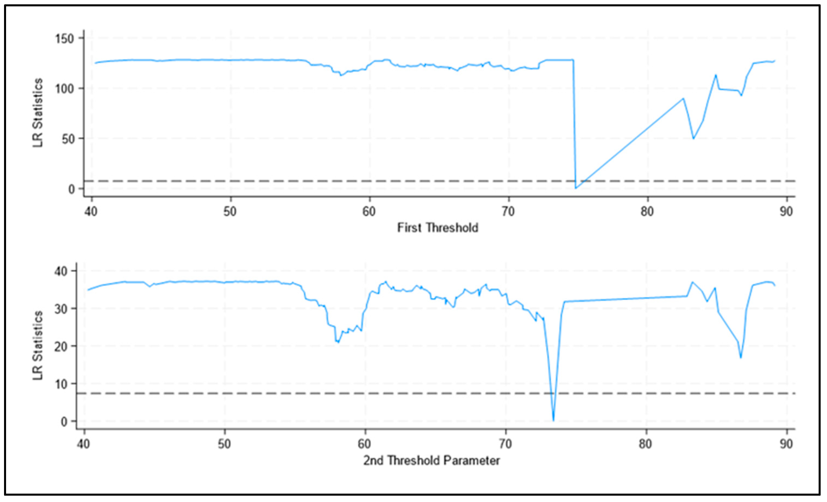
- How can interpretations of the economic-geographical threshold values explain regional developmental stage differences (Figure 3 LR plot)?
5.3.1. Threshold Effect Test
5.3.2. Threshold Value Estimation
5.3.3. Threshold Effect Regression Results
5.4. Further Analysis
5.4.1. Mediating Effect of Green Innovation
5.4.2. Regional Heterogeneity Analysis
6. Discussion, Policy Recommendations
6.1. Discussion
6.1.1. Rural Adaptability of the Digital Economy Indicator and Theoretical Contribution
6.1.2. Mechanism of Digital Economy on Agricultural Carbon Reduction: Direct Effects and Threshold Characteristics
6.1.3. Causes of Regional Heterogeneity in Spatial Spillover Effects
6.1.4. Threshold Effect of Urbanization Rate and Policy Implications
6.2. Targeted Policy Recommendations Based on Empirical Findings
6.2.1. Optimization of Green Innovation Mediation: Fund “Digital–Green” Technology Integration
6.2.2. Strengthen Spatial Spillover: Build Inter-Regional Digital Technology Sharing Mechanisms
6.2.3. Phase-Specific Policies for Urbanization Thresholds
6.2.4. Differentiated Policies for Regional Heterogeneity
6.2.5. Adjust Fiscal Support to Avoid High-Carbon Bias
7. Research Conclusions
7.1. The Above Research Yields the Following Conclusions:
- (1)
- Verification of H1: Results from the linear regression model indicate that development of the digital economy exerts a significant, direct inhibitory effect on agricultural carbon emissions. Notably, elevations in digital economy levels reduce agricultural carbon emissions, mainly through optimizing agricultural production processes, enhancing resource utilization efficiency, and by reducing traditional high-carbon factor inputs (e.g., excessive chemical fertilizers and fossil energy in farming).
- (2)
- Verification of H2: Results from the mediating effect model further reveal that the digital economy indirectly curbs carbon emissions by promoting green technological innovation in the agricultural sector. Specifically, increases in green invention patents (e.g., patents for low-carbon agricultural machinery or water-saving technologies) are significantly linked to reductions in agricultural carbon emissions, thus forming a “dual emission reduction pathway” consisting of direct inhibition by the digital economy itself and indirect reduction via green innovation.
- (3)
- Verification of H3: Findings from the Spatial Durbin Model (SDM) demonstrate that development of the digital economy conveys cross-regional synergistic effects on agricultural carbon reduction. II Increases in the digital economy levels of neighboring regions (measured by W × DE) significantly suppresses local agricultural carbon emissions. This spatial spillover effect is achieved via technology diffusion (e.g., sharing of smart agricultural solutions), market integration (unified circulation of low-carbon agricultural inputs), and regional policy coordination (joint formulation of agricultural carbon reduction targets). Such an effect underscores the critical role of inter-regional cooperation. Subsample regression results reveal that the inhibitory effect of the digital economy on agricultural carbon emissions is most pronounced in China’s Western region, while an insignificant effect is observed in the Eastern region. This discrepancy is potentially attributable to the Western region having a higher share of traditional agriculture in its agricultural production and greater room for digital technology application. In contrast, the Eastern region, which already possesses a relatively advanced agricultural modernization, has a smaller marginal effect of digital technology on carbon reduction. In addition, the impacts of control variables such as rural population size and urbanization rates also vary across regions (i.e., rural population contraction in the East weakens the pressure of high-carbon farming, while in the West, it has a more limited impact).
- (4)
- Verification of H4: Threshold effect analysis indicates that when urbanization rates cross certain thresholds, the carbon reduction effect of the digital economy exhibits nonlinear leap-forward features. This implies that the digital economy can only fully unleash its potential to drive agricultural low-carbon transformation when a region’s urbanization reaches a certain level (e.g., with mature infrastructure for connecting urban technology and rural agriculture) as opposed to exerting a linear incremental effect.
7.2. Limitations of the Study
7.3. Scientific and Social Justification of the Research
7.3.1. Scientific Justification
7.3.2. Social Justification
Author Contributions
Funding
Institutional Review Board Statement
Informed Consent Statement
Data Availability Statement
Conflicts of Interest
References
- Huang, Z.J.; Zhou, H.; Miao, Z.J.; Tang, H.; Lin, B.R.; Zhuang, W.M. Life-Cycle Carbon Emissions (LCCE) of Buildings: Implications, Calculations, and Reductions. Engineering 2024, 35, 115–139. [Google Scholar] [CrossRef]
- Jha, A.K.; Darlami, H.B.; Bhattarai, N.; Karn, S.; Neupane, G. Projecting Energy Demand and GHG Reduction With Electric Vehicle Adoption in Nepal. Appl. Eng. Lett. 2025, 10, 160–170. [Google Scholar]
- Ricke, K.L.; McCord, G.C. Tackling poverty need not impede climate action. Nature 2023, 623, 924–925. [Google Scholar] [CrossRef]
- Abulaiti, A.; She, D.L.; Pan, Y.C.; Shi, Z.Q.; Hu, L.; Huang, X.; Shan, J.; Xia, Y.Q. Drainage ditches are significant sources of indirect N2O emissions regulated by available carbon to nitrogen substrates in salt-affected farmlands. Water Res. 2024, 251, 121164. [Google Scholar] [CrossRef]
- Song, S.X.; Zhao, S.Y.; Zhang, Y.; Ma, Y.X. Carbon Emissions from Agricultural Inputs in China over the Past Three Decades. Agriculture 2023, 13, 919. [Google Scholar] [CrossRef]
- Wang, W.; Yin, X.; Wang, C.; Zhuo, M. Urban expansion and agricultural carbon emission efficiency: The moderating role of land property rights stability. J. Clean. Prod. 2025, 486, 144488. [Google Scholar] [CrossRef]
- Tian, Y.; Zhang, J.B.; He, Y.Y. Research on Spatial-Temporal Characteristics and Driving Factor of Agricultural Carbon Emissions in China. J. Integr. Agric. 2014, 13, 1393–1403. [Google Scholar] [CrossRef]
- Liu, G.; Deng, X.Z.; Zhang, F. The spatial and source heterogeneity of agricultural emissions highlight necessity of tailored regional mitigation strategies. Sci. Total Environ. 2024, 914, 169917. [Google Scholar] [CrossRef]
- Bai, L.; Guo, T.R.; Xu, W.; Liu, Y.B.; Kuang, M.; Jiang, L. Effects of digital economy on carbon emission intensity in Chinese cities: A life-cycle theory and the application of non-linear spatial panel smooth transition threshold model. Energy Policy 2023, 183. [Google Scholar] [CrossRef]
- Li, K.; Wang, H.; Xie, X. Mechanism and spatial spillover effect of the digital economy on urban carbon Productivity: Evidence from 271 prefecture-level cities in China. J. Environ. Manag. 2025, 382, 125435. [Google Scholar] [CrossRef]
- Liang, C.; Chen, X.; Di, Q. Path to pollution and carbon reduction synergy from the perspective of the digital economy: Fresh evidence from 292 prefecture-level cities in China. Environ. Res. 2024, 252, 119050. [Google Scholar] [CrossRef]
- Zuo, S.; Zhao, Y.; Zheng, L.; Zhao, Z.; Fan, S.; Wang, J. Assessing the influence of the digital economy on carbon emissions: Evidence at the global level. Sci. Total Environ. 2024, 946, 174242. [Google Scholar] [CrossRef] [PubMed]
- Wang, R.; Zhao, W. Synergistic dance of digital economy and green finance on carbon emissions: Insights from China. Chin. J. Popul. Resour. Environ. 2024, 22, 213–229. [Google Scholar] [CrossRef]
- Huang, C.C.; Lin, B.Q. Digital economy solutions towards carbon neutrality: The critical role of energy efficiency and energy structure transformation. Energy 2024, 306, 132524. [Google Scholar] [CrossRef]
- Zhu, Q.; Xu, C.; Wu, L.; Fang, X.; Pan, Y.; Zhou, D. Enhancing sustainability: Assessing the low-carbon impact of China’s digital economy on residential carbon emissions. Environ. Dev. 2025, 54, 101161. [Google Scholar] [CrossRef]
- Lin, Q.; Jian, Y.; Zhang, D.; Li, J.; Mao, S. Exploring the “Double-Edged Sword” effect of the digital economy on sustainable agricultural development: Evidence from China. Sustain. Horiz. 2025, 13, 100122. [Google Scholar] [CrossRef]
- Zhu, S.Y.; Huang, J.W.; Li, Y.S.; Maneejuk, P.; Liu, J.X. A Non-Linear Exploration of the Digital Economy’s Impact on Agricultural Carbon Emission Efficiency in China. Agriculture 2024, 14, 2245. [Google Scholar] [CrossRef]
- Wang, W.; Wu, Y.; He, X.; Wu, R. New marine productivity empowers green development of the marine economy: Theoretical mechanism and empirical evidence. Reg. Stud. Mar. Sci. 2025, 82, 104042. [Google Scholar] [CrossRef]
- Jin, M.; Feng, Y.; Wang, S.; Chen, N.; Cao, F. Can the development of the rural digital economy reduce agricultural carbon emissions? A spatiotemporal empirical study based on China’s provinces. Sci. Total Environ. 2024, 939, 173437. [Google Scholar] [CrossRef]
- Anam, M.Z.; Islam, M.H.; Islam, M.T.; Bari, A.B.M.M.; Raihan, A. A Fermatean fuzzy approach to analyze the drivers of digital transformation in the agricultural production sector: A pathway to sustainability for emerging economies. Green Technol. Sustain. 2025, 3, 100197. [Google Scholar] [CrossRef]
- E Porter, M.; van der Linde, C. Toward a New Conception of the Environment-Competitiveness Relationship. J. Econ. Perspect. 1995, 9, 97–118. [Google Scholar] [CrossRef]
- Chen, Z.; Zhang, X.; Chen, F. Do carbon emission trading schemes stimulate green innovation in enterprises? Evidence from China. Technol. Forecast. Soc. Change 2021, 168, 120744. [Google Scholar] [CrossRef]
- Fabiani, S.; Vanino, S.; Napoli, R.; Zajíček, A.; Duffková, R.; Evangelou, E.; Nino, P. Assessment of the economic and environmental sustainability of Variable Rate Technology (VRT) application in different wheat intensive European agricultural areas. A Water energy food nexus approach. Environ. Sci. Policy 2020, 114, 366–376. [Google Scholar] [CrossRef]
- Varzaru, A.A. Assessing Agricultural Impact on Greenhouse Gases in the European Union: A Climate-Smart Agriculture Perspective. Agronomy 2024, 14, 821. [Google Scholar] [CrossRef]
- Bullock, D.S.; Mieno, T.; Hwang, J. The value of conducting on-farm field trials using precision agriculture technology: A theory and simulations. Precis. Agric. 2020, 21, 1027–1044. [Google Scholar] [CrossRef]
- Wang, T.; Zhang, X.; Chen, W.; Fu, Z.; Peng, Z. RFID-based temperature monitoring system of frozen and chilled tilapia in cold chain logistics. Trans. Chin. Soc. Agric. Eng. 2011, 27, 141–146. [Google Scholar]
- Uyar, H.; Papanikolaou, A.; Kapassa, E.; Touloupos, M.; Rizou, S. Blockchain-enabled traceability and certification for frozen food supply chains: A conceptual design. Smart Agric. Technol. 2025, 12, 101085. [Google Scholar] [CrossRef]
- North, D. Competing Technologies, Increasing Returns, and Lock-In by Historical Events; University of Michigan Press: Ann Arbor, MI, USA, 1994. [Google Scholar]
- Li, L.; Chen, J.; Nie, J.; Gao, Z. Reinforcement learning energy management control strategy of electric tractor based on condition identification. Int. J. Electr. Power Energy Syst. 2025, 170, 110846. [Google Scholar] [CrossRef]
- Wiebe, K.S.; Lutz, C. Endogenous technological change and the policy mix in renewable power generation. Renew. Sustain. Energy Rev. 2016, 60, 739–751. [Google Scholar] [CrossRef]
- Bocean, C.G. The Role of Organic Farming in Reducing Greenhouse Gas Emissions from Agriculture in the European Union. Agronomy 2025, 15, 198. [Google Scholar] [CrossRef]
- Bozzo, M.B.; Tomassini, C. Collaboration networks in agricultural research in Uruguay: An exploration based on social network analysis. Outlook Agric. 2024, 53, 177–188. [Google Scholar] [CrossRef]
- Chang, Y.; Chen, L.Y.; Zhou, Y.; Meng, Q.G. Elements, characteristics, and performances of inter-enterprise knowledge recombination: Empirical research on green innovation adoption in China’s heavily polluting industry. J. Environ. Manag. 2022, 310, 114736. [Google Scholar] [CrossRef]
- Xu, B.W.; Balezentis, T.; Streimikiene, D.; Shen, Z.Y. Enhancing agricultural environmental performance: Exploring the interplay of agricultural productive services, resource allocation, and marketization factors. J. Clean. Prod. 2024, 439. [Google Scholar] [CrossRef]
- Manning, N.; Li, Y.; Liu, J. Broader applicability of the metacoupling framework than Tobler’s first law of geography for global sustainability: A systematic review. Geogr. Sustain. 2023, 4, 6–18. [Google Scholar] [CrossRef]
- Zhang, S.H.; Wen, X.W.; Sun, Y.; Xiong, Y.L. Impact of agricultural product brands and agricultural industry agglomeration on agricultural carbon emissions. J. Environ. Manag. 2024, 369, 122238. [Google Scholar] [CrossRef] [PubMed]
- Li, Y.; You, X.; Fu, J.; Zhou, W. Mechanisms and effects of the digital economy on agricultural modernization: A sustainable development perspective. J. Environ. Manag. 2025, 392, 126790. [Google Scholar] [CrossRef] [PubMed]
- Cheng, Q.; Peng, C.; Wan, H.; Dai, Y.; Zhang, S. How to realize digital knowledge innovation through digital technology? A perspective based on knowledge digitization and inter-organizational knowledge sharing. Technol. Soc. 2025, 82, 102905. [Google Scholar] [CrossRef]
- Zhang, N.; Yang, W.; Ke, H. Does rural e-commerce drive up incomes for rural residents? Evidence from Taobao villages in China. Econ. Anal. Policy 2024, 82, 976–998. [Google Scholar] [CrossRef]
- Willett, J. Challenging peripheralising discourses: Using evolutionary economic geography and, complex systems theory to connect new regional knowledges within the periphery. J. Rural. Stud. 2020, 73, 87–96. [Google Scholar] [CrossRef]
- Hu, X.Q.; Cai, J.H.; Yue, X.H. Power structure preferences in a dual-channel supply chain: Demand information symmetry vs. asymmetry. Eur. J. Oper. Res. 2024, 314, 920–934. [Google Scholar] [CrossRef]
- Zhang, J.; Gong, X.; Cheng, M. Broadband cities: Bridging urban-rural consumption gap with digital innovation. Cities 2025, 167, 106315. [Google Scholar] [CrossRef]
- Cheng, C.; Gao, Q.; Ju, K.; Ma, Y. How digital skills affect farmers’ agricultural entrepreneurship? An explanation from factor availability. J. Innov. Knowl. 2024, 9, 100477. [Google Scholar] [CrossRef]
- Guenduez, A.A.; Demircioglu, M.A.; Mueller, E.M.; Cinar, E. Digital innovation strategies in the public sector. Res. Policy 2025, 54, 105274. [Google Scholar] [CrossRef]
- Kibinda, N.; Shao, D.; Mwogosi, A.; Mambile, C. Broadband infrastructure sharing as a catalyst for rural digital economy: A systematic review for developing countries. Telecommun. Policy 2025, 103028. [Google Scholar] [CrossRef]
- Tian, Y.; Zuo, S.; Ju, J.; Dai, S.; Ren, Y.; Dou, P. Local carbon emission zone construction in the highly urbanized regions: Application of residential and transport CO2 emissions in Shanghai, China. Build. Environ. 2024, 247, 111007. [Google Scholar] [CrossRef]
- Khan, K.; Su, C.-W. Urbanization and carbon emissions: A panel threshold analysis. Environ. Sci. Pollut. Res. 2021, 28, 26073–26081. [Google Scholar] [CrossRef]
- Feng, Y.; Liu, Y.; Yuan, H. The spatial threshold effect and its regional boundary of new-type urbanization on energy efficiency. Energy Policy 2022, 164, 112866. [Google Scholar] [CrossRef]
- Du, W.; Xia, X. How does urbanization affect GHG emissions? A cross-country panel threshold data analysis. Appl. Energy 2018, 229, 872–883. [Google Scholar] [CrossRef]
- Chen, Z.; Zhou, M. Urbanization and energy intensity: Evidence from the institutional threshold effect. Environ. Sci. Pollut. Res. 2021, 28, 11142–11157. [Google Scholar] [CrossRef] [PubMed]
- Hou, J.; Li, X.; Chen, F.; Hou, B. The effect of digital economy on rural environmental governance: Evidence from China. Agriculture 2024, 14, 1974. [Google Scholar] [CrossRef]
- Yang, C.; Ji, X.; Cheng, C.; Liao, S.; Bright, O.; Zhang, Y. Digital economy empowers sustainable agriculture: Implications for farmers’ adoption of ecological agricultural technologies. Ecol. Indic. 2024, 159, 111723. [Google Scholar] [CrossRef]
- Xu, X.; Yang, H.; Yang, H. The threshold effect of agricultural energy consumption on agricultural carbon emissions: A comparison between relative poverty regions and other regions. Environ. Sci. Pollut. Res. 2021, 28, 55592–55602. [Google Scholar] [CrossRef]
- Zou, S.; Fan, X.; Wang, L.; Cui, Y. High-speed rail new towns and their impacts on urban sustainable development: A spatial analysis based on satellite remote sensing data. Humanit. Soc. Sci. Commun. 2024, 11, 894. [Google Scholar] [CrossRef]
- Gao, Y.; Cai, M.; He, X. Influence of Financial Support to Agriculture on Carbon Emission Intensity of the Industry. Sustainability 2023, 15, 2228. [Google Scholar] [CrossRef]
- Anselin, L. Handbook of spatial analysis in the social sciences. Spat. Econom. 2022, 101–122. [Google Scholar] [CrossRef]
- Hansen, B.E. Threshold effects in non-dynamic panels: Estimation, testing, and inference. J. Econom. 1999, 93, 345–368. [Google Scholar] [CrossRef]
- Zhang, X.; Li, W. The impact of digital inclusive finance on agricultural carbon emissions at the city level in China: The role of rural entrepreneurship and agricultural innovation. J. Clean. Prod. 2025, 505, 145469. [Google Scholar] [CrossRef]
- Zhang, Y.; Khan, S.U.; Wang, Y. The future is digital: Can the digital economy drive marine sustainability? Exploring regional impacts on fisheries’ carbon emissions in coastal China. J. Clean. Prod. 2025, 506, 145518. [Google Scholar] [CrossRef]


| Main Agricultural Input | Emission Coefficient | Data Source |
|---|---|---|
| Diesel | 0.5927 kg/kg | IPCC (2007) |
| Plastic Film | 5.18 kg/kg | Nanjing Agricultural University Institute |
| Fertilizer | 0.895 kg/kg | Oak Ridge National Laboratory |
| Pesticide | 4.9341 kg/kg | Oak Ridge National Laboratory |
| Irrigated Area | 25 kg/hm2 | USDA Dubay Laboratory |
| Crop Cultivation Area | 3.126 kg/hm2 | China Agricultural University Biotechnology Inst |
| Dimension | Secondary Indicators | Weight |
|---|---|---|
| Digital Infrastructure | Number of Internet Broadband Access Ports | 0.0963 |
| Number of Internet Broadband Subscribers | 0.1069 | |
| Mobile Phone Penetration Rate | 0.0457 | |
| Digital Industrialization | Software Business Revenue as % of GDP | 0.2381 |
| IT Service Revenue as % of GDP | 0.2703 | |
| Employment in Information Services | 0.1858 | |
| Industrial Digitization | Number of Websites per 100 Enterprises | 0.0390 |
| Proportion of Enterprises Engaged in E-commerce | 0.0179 |
| Secondary Indicator | PCA Loading (First Component) |
|---|---|
| Internet Broadband Access Ports | 0.896 |
| Internet Broadband Subscribers | 0.872 |
| Mobile Phone Penetration Rate | 0.795 |
| Software Revenue/GDP | 0.921 |
| IT Service Revenue/GDP | 0.887 |
| Information Service Employment | 0.763 |
| Websites per 100 Enterprises | 0.814 |
| E-commerce Enterprise Proportion | 0.789 |
| Variable Category | Variable Name (Abbreviation) | Core Definition | Data Source | Statistical Period | Statistical Caliber |
|---|---|---|---|---|---|
| Dependent Variable | Agricultural Carbon Emissions (ACE) | Total carbon emissions from 6 agricultural carbon sources (diesel, plastic film, etc.) | China Rural Statistical Yearbook; IPCC (2007); Nanjing Agricultural University | 2013–2022 | Provincial-level, calculated via emission coefficient method (Unit: 10,000 tons) |
| Core Explanatory Variable | Digital Economy Index (DE) | Comprehensive index of digitalization (3 dimensions: infrastructure, industrialization, digitization) | China Statistical Yearbook; China Communication Statistical Yearbook; EPS Database | 2013–2022 | Provincial-level, composite index via entropy weight method (Dimensionless) |
| Mediating Variable | Green Innovation (GI) | Level of green technology innovation | China Science and Technology Statistical Yearbook; EPS Database (Patent Module) | 2013–2022 | Provincial-level, number of agricultural green invention patent applications (Unit: Piece) |
| Control Variables | Rural Population Size (Rps) | Scale of rural resident population | China Rural Statistical Yearbook | 2013–2022 | Provincial-level (Unit: 10,000 persons) |
| Rural Electricity Consumption (Rec) | Total electricity consumption in rural areas (agricultural + residential) | China Energy Statistical Yearbook | 2013–2022 | Provincial-level (Unit: 100 million kWh) | |
| Urbanization Rate (Ur) | Proportion of urban population to total population | China Statistical Yearbook | 2013–2022 | Provincial-level (Unit: %) | |
| Fiscal Expenditure on Agriculture (Fsa) | Proportion of agricultural fiscal expenditure to total fiscal expenditure | China Fiscal Statistical Yearbook | 2013–2022 | Provincial-level (Unit: %) | |
| Agricultural Added Value (Aav) | Proportion of primary industry added value to regional GDP | China Statistical Yearbook | 2013–2022 | Provincial-level (Unit: %) |
| Variables | Quantity | Provinces |
|---|---|---|
| Rural Electricity Consumption (Rec) | 2 missing observations | Qinghai, 2013; Ningxia, 2014 |
| Variables | N | Mean | Std. Dev. | Min | Max | Unit |
|---|---|---|---|---|---|---|
| DE | 300 | 0.157 | 0.111 | 0.0242 | 0.688 | Dimensionless |
| ACE | 300 | 335.0 | 227.0 | 13.91 | 995.7 | 10,000 tons |
| GI | 300 | 4894 | 6833 | 31 | 45,359 | Piece |
| Rps | 300 | 1831 | 1234 | 203 | 5399 | 10,000 persons |
| Rec | 300 | 278.7 | 376.6 | 4.500 | 1949 | 100 million kWh |
| Ur | 300 | 61.39 | 11.38 | 37.89 | 89.60 | Percentage (%) |
| Fsa | 300 | 11.45 | 3.447 | 4.040 | 20.38 | Percentage (%) |
| Aav | 300 | 9.590 | 5.300 | 0.220 | 25.27 | Percentage (%) |
| (1) | (2) | (3) | (4) | (5) | (6) | |
|---|---|---|---|---|---|---|
| Variables | LnACE | LnACE | LnACE | LnACE | LnACE | LnACE |
| DE | −1.622 *** | −2.565 *** | −3.058 *** | −2.559 *** | −2.325 *** | −2.051 *** |
| (−2.99) | (−7.53) | (−8.19) | (−4.60) | (−4.42) | (−4.01) | |
| Rps | 0.001 *** | 0.001 *** | 0.001 *** | 0.001 *** | 0.001 *** | |
| (21.76) | (19.82) | (12.26) | (14.34) | (14.67) | ||
| Rec | 0.000 *** | 0.000 *** | 0.000 *** | 0.000 *** | ||
| (3.03) | (3.27) | (3.39) | (3.91) | |||
| Ur | −0.008 | 0.016 ** | 0.022 *** | |||
| (−1.21) | (2.28) | (3.05) | ||||
| Fsa | 0.098 *** | 0.065 *** | ||||
| (6.09) | (3.76) | |||||
| Aav | 0.047 *** | |||||
| (4.66) | ||||||
| Constant | 5.695 *** | 4.627 *** | 4.665 *** | 5.126 *** | 2.269 *** | 1.848 *** |
| (54.69) | (56.93) | (57.50) | (13.14) | (3.81) | (3.17) | |
| Observations | 300 | 300 | 300 | 300 | 300 | 300 |
| R-squared | 0.029 | 0.626 | 0.637 | 0.639 | 0.679 | 0.701 |
| Variables | DE | LnACE |
|---|---|---|
| L.DE | 0.984 *** | |
| (45.636) | ||
| DE | −2.196 *** | |
| (−3.884) | ||
| CVs | Yes | Yes |
| F | 2082.656 | 103.881 |
| CD Wald F | 2082.656 | |
| SW S stat. | 14.168 | |
| N | 270 | 270 |
| Variables | <2018 | ≥2018 |
|---|---|---|
| DE | −3.184 *** | −2.657 *** |
| (−3.24) | (−3.77) | |
| Rps | 0.001 *** | 0.001 *** |
| (11.08) | (9.70) | |
| Rec | 0.000 *** | 0.001 *** |
| (3.51) | (2.86) | |
| Ur | 0.024 ** | 0.029 ** |
| (2.58) | (2.20) | |
| Fsa | 0.090 *** | 0.053 ** |
| (3.55) | (2.01) | |
| Aav | 0.042 *** | 0.046 *** |
| (3.19) | (3.06) | |
| Constant | 1.592 ** | 1.471 |
| (2.06) | (1.33) | |
| Observations | 150 | 150 |
| R-squared | 0.730 | 0.703 |
| Variables | LnACE |
|---|---|
| Pca_DE | −4.557 *** |
| (0.572) | |
| Cons | 8.697 *** |
| (0.413) | |
| N | 300 |
| R-squared | 0.175 |
| adj. R-squared | 0.173 |
| Year | Adjacency Matrix W1 | Geographic Distance Matrix W2 | ||
|---|---|---|---|---|
| LnACE | Z-Value | LnACE | Z-Value | |
| 2013 | 0.240 ** | 2.506 | 0.190 | 1.584 |
| 2014 | 0.218 ** | 2.302 | 0.188 | 1.565 |
| 2015 | 0.207 ** | 2.204 | 0.186 | 1.553 |
| 2016 | 0.199 ** | 2.128 | 0.190 | 1.577 |
| 2017 | 0.195 ** | 2.091 | 0.196 | 1.621 |
| 2018 | 0.192 ** | 2.067 | 0.204 * | 1.674 |
| 2019 | 0.187 ** | 2.015 | 0.208 * | 1.705 |
| 2020 | 0.189 ** | 2.036 | 0.216 * | 1.761 |
| 2021 | 0.182 ** | 1.963 | 0.215 * | 1.745 |
| 2022 | 0.166 * | 1.821 | 0.212 * | 1.724 |
| Year | Adjacency Matrix W1 | Geographic Distance Matrix W2 | ||
|---|---|---|---|---|
| LnDE | Z-Value | LnDE | Z-Value | |
| 2013 | 0.2333 ** | 2.1948 | 0.0374 ** | 2.0554 |
| 2014 | 0.2476 ** | 2.3226 | 0.0439 ** | 2.2528 |
| 2015 | 0.2372 ** | 2.2311 | 0.0290 * | 1.8177 |
| 2016 | 0.2984 *** | 2.7272 | 0.0481 ** | 2.3622 |
| 2017 | 0.2538 ** | 2.3654 | 0.0191 | 1.5355 |
| 2018 | 0.2539 ** | 2.3739 | 0.0220 | 1.6231 |
| 2019 | 0.3382 *** | 3.0872 | 0.0462 ** | 2.3328 |
| 2020 | 0.3636 *** | 3.3174 | 0.0601 *** | 2.7494 |
| 2021 | 0.4460 *** | 3.9391 | 0.0796 *** | 3.2644 |
| 2022 | 0.4199 *** | 3.7570 | 0.0730 *** | 3.1020 |
| Test Type | Statistic | p Value | Test Type | Statistic | p Value |
|---|---|---|---|---|---|
| LM-error | 498.152 *** | 0.000 | Wald–spatial lag | 31.92 *** | 0.000 |
| Robust LM-error | 335.205 *** | 0.000 | LR–spatial lag | 59.42 *** | 0.000 |
| LM-lag | 171.110 *** | 0.000 | Wald–spatial error | 52.73 *** | 0.000 |
| Robust LM-lag | 8.163 *** | 0.004 | LR–spatial error | 60.04 *** | 0.000 |
| Hausman | 66.50 *** | 0.000 |
| Test Type | Statistic | p Value | Test Type | Statistic | p Value |
|---|---|---|---|---|---|
| LM-error | 279.672 *** | 0.000 | Wald–spatial lag | 66.45 *** | 0.000 |
| Robust LM-error | 102.243 *** | 0.000 | LR–spatial lag | 70.24 *** | 0.000 |
| LM-lag | 180.566 *** | 0.000 | Wald–spatial error | 76.14 *** | 0.000 |
| Robust LM-lag | 3.237 * | 0.072 | LR–spatial error | 66.62 *** | 0.000 |
| Hausman | 46.27 *** | 0.000 |
| Variables | Adjacency Matrix W1 | Geographic Distance Matrix W2 |
|---|---|---|
| ω | 0.513 *** (0.0866) | 0.480 *** (0.0965) |
| DE | −0.0548 (0.142) | −0.0747 (0.154) |
| Rps | −6.80 × 10⁻⁷ (6.93 ×10⁻⁵) | 8.18 ×10⁻⁵ (6.35 ×10⁻⁵) |
| Rec | 1.20 ×10⁻⁵ (5.19 ×10⁻⁵) | 1.42 ×10⁻⁵ (4.51 ×10⁻⁵) |
| Ur | 0.0122 ** (0.00583) | 0.0210 *** (0.00776) |
| Fsa | −0.000403 (0.00369) | 0.00613 (0.00433) |
| Aav | −0.0215 *** (0.00726) | −0.0103 * (0.00621) |
| sigma2_e | 0.00203 *** (0.000380) | 0.00222 *** (0.000496) |
| W × DE | −0.702 *** (0.229) | −1.396 *** (0.251) |
| W × Rps | 0.000182 (0.000162) | −0.000312 * (0.000173) |
| W × Rec | 3.97 ×10⁻⁵ (6.89 ×10⁻⁵) | 4.75 ×10⁻⁵ (6.43 ×10⁻⁵) |
| W × Ur | −0.00557 (0.00932) | −0.0262 ** (0.0104) |
| W × Fsa | 0.00669 (0.00608) | −0.00447 (0.00972) |
| W × Aav | 0.0114 (0.0111) | −0.00936 (0.0103) |
| R-squared | 0.079 | 0.106 |
| Observations | 300 | 300 |
| Variables | Adjacency Matrix W1 | Geographic Distance Matrix W2 | ||||
|---|---|---|---|---|---|---|
| Direct Effect | Indirect Effect | Total Effect | Direct Effect | Indirect Effect | Total Effect | |
| DE | −0.172 | −1.434 ** | −1.607 ** | −0.222 | −2.708 *** | −2.930 *** |
| (0.167) | (0.605) | (0.708) | (0.159) | (0.712) | (0.753) | |
| Rps | 2.66 ×10⁻⁵ | 0.000359 | 0.000386 | 4.98 ×10⁻⁵ | −0.000522 | −0.000472 |
| (6.71 ×10⁻⁵) | (0.000291) | (0.000310) | (6.80 ×10⁻⁵) | (0.000345) | (0.000379) | |
| Rec | 2.46 ×10⁻⁵ | 8.70 ×10⁻⁵ | 0.000112 | 2.50 ×10⁻⁵ | 0.000106 | 0.000131 |
| (5.08 ×10⁻⁵) | (0.000118) | (0.000138) | (4.51 ×10⁻⁵) | (0.000127) | (0.000150) | |
| Ur | 0.0122 ** | 0.00232 | 0.0145 | 0.0191 *** | −0.0291 * | −0.0101 |
| (0.00523) | (0.0152) | (0.0153) | (0.00717) | (0.0164) | (0.0154) | |
| Fsa | 0.000691 | 0.0116 | 0.0123 | 0.00591 | −0.00245 | 0.00346 |
| (0.00338) | (0.00952) | (0.00984) | (0.00390) | (0.0165) | (0.0161) | |
| Test Type | Statistic | p Value | Test Type | Statistic | p Value |
|---|---|---|---|---|---|
| LM-error | 76.394 *** | 0.000 | Wald–spatial lag | 35.96 *** | 0.000 |
| Robust LM-error | 36.374 *** | 0.000 | LR–spatial lag | 49.36 *** | 0.000 |
| LM-lag | 42.797 *** | 0.000 | Wald–spatial error | 52.73 *** | 0.000 |
| Robust LM-lag | 2.776 * | 0.096 | LR–spatial error | 38.02 *** | 0.000 |
| Hausman | 343.10 *** | 0.000 |
| Variables | SDM | Direct | Indirect | Total |
|---|---|---|---|---|
| W × DE | −2.713 ** | |||
| (1.330) | ||||
| DE | −2.439 *** | −2.640 *** | −5.085 *** | −7.725 *** |
| (0.537) | (0.530) | (1.847) | (1.973) | |
| Rps | 0.001 *** | 0.001 *** | 0.001 *** | 0.001 *** |
| (0.000) | (0.000) | (0.000) | (0.000) | |
| Rec | 0.001 *** | 0.001 *** | −0.000 | 0.000 |
| (0.000) | (0.000) | (0.000) | (0.001) | |
| Ur | 0.021 *** | 0.020 *** | −0.013 | 0.007 |
| (0.008) | (0.008) | (0.031) | (0.033) | |
| Fsa | 0.031 * | 0.010 | −0.453 *** | −0.444 *** |
| (0.018) | (0.022) | (0.110) | (0.124) | |
| Aav | 0.067 *** | 0.073 *** | 0.096 | 0.169 ** |
| (0.011) | (0.014) | (0.075) | (0.086) | |
| rho | 0.324 *** | |||
| (0.106) | ||||
| sigma2_e | 0.249 *** | |||
| (0.020) | ||||
| Observations | 300 | 300 | 300 | 300 |
| R-squared | 0.609 | 0.609 | 0.609 | 0.609 |
| Number of id | 30 | 30 | 30 | 30 |
| Threshold Variable | Number of Thresholds | F-Value | p-Value | Critical Value 10% | Critical Value 5% | Critical Value 1% |
|---|---|---|---|---|---|---|
| Urbanization Rate | Single Threshold | 132.82 | 0.0000 | 32.9855 | 39.2544 | 48.2278 |
| Double Threshold | 38.21 | 0.0167 | 24.5453 | 27.8955 | 40.4832 |
| Threshold Variable | Threshold Number | Estimated Value | 95% Confidence Interval |
|---|---|---|---|
| Urbanization Rate | Single Threshold | 73.38 | [73.0000, 73.4400] |
| Double Threshold | 74.79 | [74.6300, 82.2900] |
| Variables | LnACE |
|---|---|
| 0.ur | −0.00731 *** |
| (−3.791) | |
| 1.ur | −0.00385 *** |
| (−1.865) | |
| 2.ur | −0.208 *** |
| (−10.98) | |
| Constant | 7.538 *** |
| (31.99) | |
| Observations | 300 |
| R-squared | 0.698 |
| Variables | (1) | (2) | (3) |
|---|---|---|---|
| LnACE | Lngi | LnACE | |
| DE | −2.0510 *** | 3.7657 *** | −3.947 *** |
| (−4.0056) | (7.8179) | (0.497) | |
| lngi | 0.503 *** | ||
| (0.0548) | |||
| rps | 0.0007 *** | 0.0007 *** | 0.000356 *** |
| (14.6749) | (15.1675) | (5.60e−05) | |
| rec | 0.0004 *** | −0.0000 | 0.000456 *** |
| (3.9140) | (−0.2697) | (9.96e−05) | |
| ur | 0.0216 *** | 0.0728 *** | −0.0151 ** |
| (3.0532) | (10.9564) | (0.00740) | |
| fsa | 0.0648 *** | 0.0318 * | 0.0488 *** |
| (3.7646) | (1.9638) | (0.0153) | |
| aav | 0.0468 *** | −0.0188 ** | 0.0563 *** |
| (4.6567) | (−1.9910) | (0.00892) | |
| Constant | 1.8482 *** | 1.2818 ** | 1.203 ** |
| (3.1689) | (2.3362) | (0.519) | |
| Observations | 300 | 300 | 300 |
| R- squared | 0.7013 | 0.8282 | 0.768 |
| Item | Observed Coefficient | Bias | Std. Err | [95% Conf. Interval] |
|---|---|---|---|---|
| Indirect | 1.896 | 0.0281 | 0.357 | [1.317,2.719] (P) |
| [1.328,2.736] (BC) |
| Agricultural-Specific Granted Patents | Total Green Granted Patents | ||||
|---|---|---|---|---|---|
| LnACE | Lnagi | LnACE | Lnngi | LnACE | |
| DE | −2.0510 *** | 3.5005 *** | −3.6007 *** | 2.1395 *** | −2.6080 *** |
| (−4.0056) | (7.5247) | (−7.0195) | (3.3672) | (−5.2720) | |
| Lnagi | 0.4427 *** | ||||
| (7.5071) | |||||
| Lnngi | 0.2604 *** | ||||
| (5.8340) | |||||
| Rps | 0.0007 *** | 0.0006 *** | 0.0004 *** | 0.0006 *** | 0.0005 *** |
| (14.6749) | (15.0394) | (7.0656) | (9.8264) | (10.5207) | |
| Rec | 0.0004 *** | 0.0001 | 0.0004 *** | −0.0006 *** | 0.0006 *** |
| (3.9140) | (1.0796) | (3.7867) | (−4.2900) | (5.4232) | |
| Ur | 0.0216 *** | 0.0662 *** | −0.0078 | 0.0399 *** | 0.0112 |
| (3.0532) | (10.3284) | (−1.0280) | (4.5548) | (1.6122) | |
| Fsa | 0.0648 *** | 0.0307 * | 0.0512 *** | 0.0124 | 0.0615 *** |
| (3.7646) | (1.9652) | (3.2218) | (0.5806) | (3.7711) | |
| Aav | 0.0468 *** | −0.0263 *** | 0.0584 *** | 0.0055 | 0.0453 *** |
| (4.6567) | (−2.8842) | (6.2543) | (0.4433) | (4.7595) | |
| _cons | 1.8482 *** | 2.2558 *** | 0.8496 | 3.8397 *** | 0.8485 |
| (3.1689) | (4.2571) | (1.5413) | (5.3052) | (1.4658) | |
| N | 300 | 300 | 300 | 300 | 300 |
| R- squared | 0.7013 | 0.8321 | 0.7497 | 0.4658 | 0.7325 |
| DE | Lngi | |
|---|---|---|
| L.DE | 0.984 *** | |
| (45.636) | ||
| DE | 3.874 *** | |
| (7.475) | ||
| CVs | Yes | Yes |
| Cons | −0.011 | 1.842 ** |
| (−0.442) | (3.113) | |
| Obs | 270 | 270 |
| R- squared | 0.828 | |
| F | 2082.656 | 212.065 |
| CD Wald F | 2082.656 | |
| SW S stat. | 46.866 |
| Variables | (1) East LnACE | (2) Central LnACE | (3) West LnACE |
|---|---|---|---|
| DE | −0.464 | 0.133 | −6.079 ** |
| (−0.95) | (0.13) | (−2.38) | |
| Rps | 0.000407 *** | 0.000421 *** | 0.000419 ** |
| (4.86) | (5.89) | (2.94) | |
| Rec | 0.000382 *** | −0.000261 | 0.00848 *** |
| (3.78) | (−0.47) | (4.40) | |
| Ur | −0.0820 *** | 0.0228 | 0.0243 |
| (−4.55) | (1.93) | (1.60) | |
| Fsa | −0.0818 * | −0.00818 | 0.00147 |
| (−2.05) | (−0.42) | (0.05) | |
| Aav | −0.0291 | 0.0533 *** | 0.0259 |
| (−1.53) | (7.11) | (0.76) | |
| Cons | 11.03 *** | 3.287 *** | 2.759 * |
| (6.70) | (4.66) | (2.47) | |
| N | 110 | 80 | 110 |
Disclaimer/Publisher’s Note: The statements, opinions and data contained in all publications are solely those of the individual author(s) and contributor(s) and not of MDPI and/or the editor(s). MDPI and/or the editor(s) disclaim responsibility for any injury to people or property resulting from any ideas, methods, instructions or products referred to in the content. |
© 2025 by the authors. Licensee MDPI, Basel, Switzerland. This article is an open access article distributed under the terms and conditions of the Creative Commons Attribution (CC BY) license (https://creativecommons.org/licenses/by/4.0/).
Share and Cite
Lin, K.; Ye, T.; Xi, S.; Yi, C. Digital Economy, Green Innovation, and Agricultural Carbon Emission Reduction: Spillover Effects and Analyses of Mechanisms. Sustainability 2025, 17, 10420. https://doi.org/10.3390/su172210420
Lin K, Ye T, Xi S, Yi C. Digital Economy, Green Innovation, and Agricultural Carbon Emission Reduction: Spillover Effects and Analyses of Mechanisms. Sustainability. 2025; 17(22):10420. https://doi.org/10.3390/su172210420
Chicago/Turabian StyleLin, Kejun, Taobo Ye, Shilong Xi, and Chuanjian Yi. 2025. "Digital Economy, Green Innovation, and Agricultural Carbon Emission Reduction: Spillover Effects and Analyses of Mechanisms" Sustainability 17, no. 22: 10420. https://doi.org/10.3390/su172210420
APA StyleLin, K., Ye, T., Xi, S., & Yi, C. (2025). Digital Economy, Green Innovation, and Agricultural Carbon Emission Reduction: Spillover Effects and Analyses of Mechanisms. Sustainability, 17(22), 10420. https://doi.org/10.3390/su172210420