An Integrated SSA-LSTM-Transformer Model for Identifying and Predicting Driving Factors of Provincial Carbon Emissions in China

Abstract

To support China’s dual-carbon goals and sustainability-oriented mitigation planning, this study develops an SSA–LSTM–Transformer framework for provincial carbon emission forecasting and interpretable driver analysis. Using panel data for 30 provinces from 2005 to 2022, SSA is employed for adaptive hyperparameter optimization, while the LSTM captures local temporal memory and the Transformer models long-range dependencies. Ablation tests and benchmarking against eight widely used models demonstrate that the proposed framework achieves the best overall performance on the held-out test set, with R² = 0.9911 and NRMSE = 0.0192. SHAP analysis indicates that a more carbon-intensive energy structure is associated with higher predicted emissions, whereas stronger technological innovation is associated with lower predicted emissions, and feature-importance patterns vary across development-stage groups. Forecast trajectories diverge during 2025–2035 and show a convergence tendency by 2050 under the model assumptions, informing differentiated near-term mitigation pathways and longer-term cross-regional coordination and technology diffusion. The results provide an interpretable evidence base for sustainability-oriented provincial decarbonization policies.

1. Introduction

With China pursuing its dual-carbon goals, provinces are where emission-cutting policies and industrial adjustments actually take place, and they are also where differences in development and resource conditions are most visible [1]. Because these differences shape provinces’ vulnerability and adjustment capacity, non-stationary shocks, especially major public health events, can affect provincial carbon emission trajectories in different ways by disrupting energy use, mobility, and production activities, which in turn complicates trend evolution and forecast uncertainty [2]. More reliable provincial emission forecasts, along with a clear understanding of what drives changes across regions, can turn an overall cap into practical policy packages by region, sector, and time horizon [3]. This makes mitigation measures more targeted and more cost-effective. This study focuses on identifying provincial drivers and producing medium- to long-term forecasts to support differentiated emission-reduction strategies and a coordinated transition [4].

Existing province-level carbon emission forecasting studies generally fall into three groups. The first relies on statistical and econometric approaches, most often regression and panel models [5], LMDI decomposition [6], ARIMA time-series models [7], and grey forecasting [8]. These methods are transparent: the structure is easy to follow, variables have clear meanings, and results can be linked directly to drivers such as industrial structure, the energy mix, population, and urbanization. That clarity also makes policy interpretation more straightforward. The downside is limited flexibility in capturing complex data patterns [9]. Performance can drop when emissions fluctuate sharply, relationships are strongly nonlinear, or effects persist across years, and the models tend to depend more on their assumptions and on stable samples [10].

The second group uses machine learning, including support vector machines, random forests [11], SVM [12], XGBoost [13], and LightGBM [14]. With fewer prior constraints, these models can learn complicated relationships and are often better at handling multivariate interactions, nonlinear dynamics, and high-dimensional features, which can translate into higher accuracy. Their weaknesses are sensitivity to sample size and feature quality, and results can vary noticeably with different hyperparameters and training choices. Interpretability is often limited, and models may not transfer well across regions when local conditions and data distributions differ [15].

The third group follows a hybrid strategy. Common examples include combining ARIMA with LSTM, linking decomposition steps with an LSTM predictor [16], and architectures that integrate LSTM with Transformer components. These designs can capture both long-term trends and short-term variability, which is helpful for medium- and long-horizon forecasts and tends to improve stability on complex sequences [17]. The trade-off is greater structural complexity, heavier tuning effort, and stronger reliance on computation and training procedures [18]. Stacked modules can also weaken the explanatory chain, so turning results into clear, policy-relevant statements usually requires additional supporting work.

In hyperparameter tuning, most existing studies rely on grid search or random search on a validation set. These approaches are easy to implement and make comparisons straightforward, but the computational burden grows quickly as the number of parameters increases, and better combinations can still be missed [19]. To improve efficiency, some work adopts Bayesian optimization, which updates the search direction over iterations and reduces the number of trials. Its performance, however, can be sensitive to how the validation set is split and to noise in the evaluation metric. Other studies use automated metaheuristic methods for tuning, such as genetic algorithms, particle swarm optimization, and simulated annealing. These can explore a wider space and reduce reliance on manual choices, yet their stability and computational cost depend heavily on algorithm settings [20].

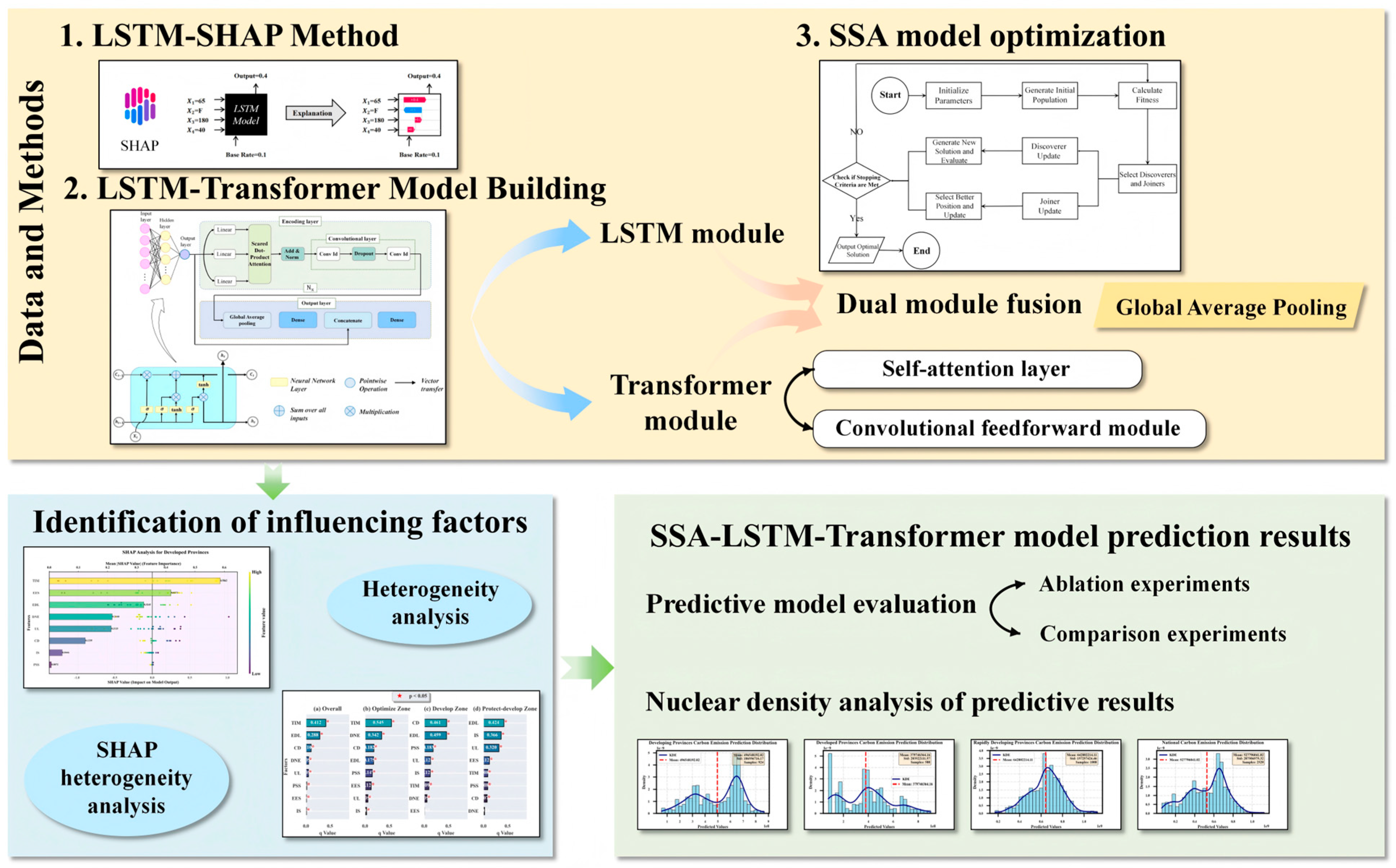
To address these issues, we develop an SSA–LSTM–Transformer forecasting framework that combines high-accuracy prediction with interpretable identification of heterogeneous provincial drivers. Methodologically, existing forecasting studies often face three practical limitations: model structures that do not simultaneously capture short-run temporal inertia and longer-range dependencies, heavy reliance on manual or heuristic hyperparameter tuning that reduces robustness and reproducibility, and limited interpretability that makes it difficult to translate predictive results into region-specific policy insights. In particular, to better accommodate complex temporal dynamics under non-stationary disturbances and possible structural changes, we integrate LSTM and Transformer components within a unified architecture. The LSTM captures recursive memory-based representations and local temporal inertia, while the Transformer uses self-attention to learn longer-range cross-period relationships and global dependencies. This complementary design improves the model’s ability to represent both short-term fluctuations and longer-horizon dynamic patterns in provincial carbon emission trajectories. To reduce uncertainty from manual tuning and enhance model robustness, we introduce the sparrow search algorithm (SSA) to adaptively optimize key hyperparameters, thereby improving convergence stability and generalization performance. On the interpretability side, we use SHAP to decompose model outputs into feature contributions and then compare these contributions across regions to identify heterogeneous driving mechanisms. In this way, the proposed framework links improved predictive performance with clearer driver interpretation. The overall framework is shown in Figure 1.

2. Model Framework and Methodology

2.1. Data Sources

This study uses a provincial panel dataset for China covering 2005–2022. The dependent variable in the forecasting analysis is total provincial carbon emissions. After excluding Hong Kong, Macao, Taiwan, and Tibet due to inconsistent statistical definitions and data completeness, the final sample contains 30 provinces over 18 years, yielding 540 province–year observations in total. For forecasting evaluation, we adopt a chronological (time-ordered) split: 2005–2017 is used for training (390 observations), 2018–2020 for validation (90 observations, used for SSA-based hyperparameter search), and 2021–2022 for testing (60 observations, held out for final evaluation). The driver system is summarized in

Table 1. Carbon emission drivers.

Indicator Factor	Abbreviation	Classify	Range	References
Regional comprehensive economic strength	EDL	Scale and Growth-Driven	[−3.78, 9.50]	[19,20]
Innovation input, R&D vitality, and sustainability potential	TIM	Structure Optimization and Efficiency Enhancement	[−5.98, 3.60]	[21,22]
Energy efficiency and green development level	EES	Structure Optimization and Efficiency Enhancement	[−4.28, 3.98]	[23]
Urban concentration and social modernization	UL	Spatial and System Characteristics	[−2.94, 4.33]	[24]
Demographic foundation and resource analysis	PSS	Scale and Growth-Driven	[−1.59, 3.04]	[25,26]
Digital infrastructure penetration and intelligent modernization	DNE	Spatial and System Characteristics	[−3.00, 1.65]	[27]
Industrial sophistication and economic transformation quality	IS	Structure Optimization and Efficiency Enhancement	[−1.64, 4.41]	[28]
Comprehensive and balanced regional coordination	CD	Spatial and System Characteristics	[−1.63, 1.76]	[29]

and spans economic development, technological innovation, energy efficiency, urbanization, population and resources, digitalization, industrial structure, and regional coordination.

Each dimension is constructed by aggregating a set of observable indicators. We first harmonize units and adjust indicator directions so that higher values consistently represent stronger performance. For indicators where lower values indicate better performance (e.g., intensity-type or gap-type indicators), the direction is reversed before standardization. After direction adjustment, all indicators are standardized using the z-score transformation:

$$z_{ijt}={\displaystyle \frac{x_{ijt}-{\mu }_j}{{\sigma }_j}},$$

(1)

where $x_{ijt}$ denotes indicator $j$ for province $i$ in year $t$, and ${\mu }_j$ and ${\sigma }_j$ are the sample mean and standard deviation of indicator $j$.

Indicators within the same dimension are then aggregated using a PCA-based weighting scheme. For each dimension, principal component analysis is performed on the standardized indicators, and the score of the $k$-th retained principal component is denoted by $F_{ikt}^{\left(g\right)}$. The composite score of dimension $g$ is calculated as a weighted sum of retained component scores:

$$S_{igt}={\sum }_{k=1}^{r_g}{w}_k{F}_{ikt}^{\left(g\right)},$$

(2)

where $r_g$ is the number of retained principal components. The component weights are determined by the explained variance (eigenvalues) of the retained components:

$$w_k={\displaystyle \frac{{\lambda }_k}{{\sum }_{m=1}^{r_g}{\lambda }_m}},$$

(3)

where ${\lambda }_k$ is the eigenvalue of the kkk-th principal component. This PCA-based aggregation provides an objective weighting rule and reduces redundancy among correlated indicators. To maintain comparability across provinces and over time, the same PCA loading structure is applied consistently when constructing yearly provincial scores within each dimension.

The dimensions are constructed as follows. EDL captures regional economic scale and growth quality and is compiled from standardized indicators including GDP per capita, the economic growth rate, fixed-asset investment intensity, and fiscal revenue or industrial value added [19,20]. TIM reflects innovation inputs and outputs, combining R&D expenditure intensity, the scale of R&D personnel, patent output, and the share of high-tech industry output [21,22]. EES measures energy efficiency and green development, based on energy consumption per unit of GDP, electricity use per unit of GDP, the share of clean energy, and GDP-related emissions intensity; indicators expressed as “intensity” are reverse-coded so that higher values indicate better performance [23]. UL represents urbanization and social modernization and is constructed from standardized measures of the urbanization rate, urban population concentration, and the provision of infrastructure and public services [24]. PSS describes population fundamentals and resource conditions, aggregating population size, employment scale, and energy-supply capacity [25,26]. DNE captures digital infrastructure and the level of smart modernization, using internet penetration, broadband access capacity, and the density of mobile communications infrastructure. IS reflects industrial upgrading and the quality of structural transformation, combining the share of the tertiary sector and the share of advanced manufacturing [27]. CD characterizes regional coordination and balance, integrating the urban–rural income gap, gaps in public services, and an index of regional development disparity [29]. Gap-type indicators are reverse-coded before aggregation so that higher scores consistently indicate stronger coordination.

We conducted a sensitivity test for the composite-indicator weighting scheme by reconstructing the indices using an equal-weight aggregation and comparing them with the PCA-based scores over the 2005–2022 panel. For the multi-indicator dimensions (EDL, TIM, EES, and DNE), the PCA-based and equal-weight scores were perfectly rank-consistent and linearly equivalent in practice (Pearson and Spearman correlations > 0.75 in all cases after direction adjustment and standardization). For UL, PSS, IS, and CD, the current specification uses a single indicator, so weighting-scheme sensitivity is not applicable. These results indicate that the composite-index construction is not sensitive to the weighting scheme under the current indicator design.

2.2. LSTM–SHAP Approach

To interpret how predictors contribute to carbon emission forecasts, we use SHAP (Shapley Additive exPlanations) to attribute the model output to additive feature contributions. SHAP is grounded in the Shapley value from cooperative game theory and quantifies the marginal contribution of each feature to the prediction under the fitted model [30]. For feature $\mathrm{i}$, the SHAP value ${\mathsf{\varphi }}_{\mathrm{i}}$ is defined as

$${\varphi }_i={\sum }_{S\subseteq \mathcal{F}\setminus \left\{i\right\}}{\displaystyle \frac{\mid S\mid !(M-\mid S\mid -1)!}{M!}}\left[v(S\cup \{i\left\}\right)-v\left(S\right)\right],$$

(4)

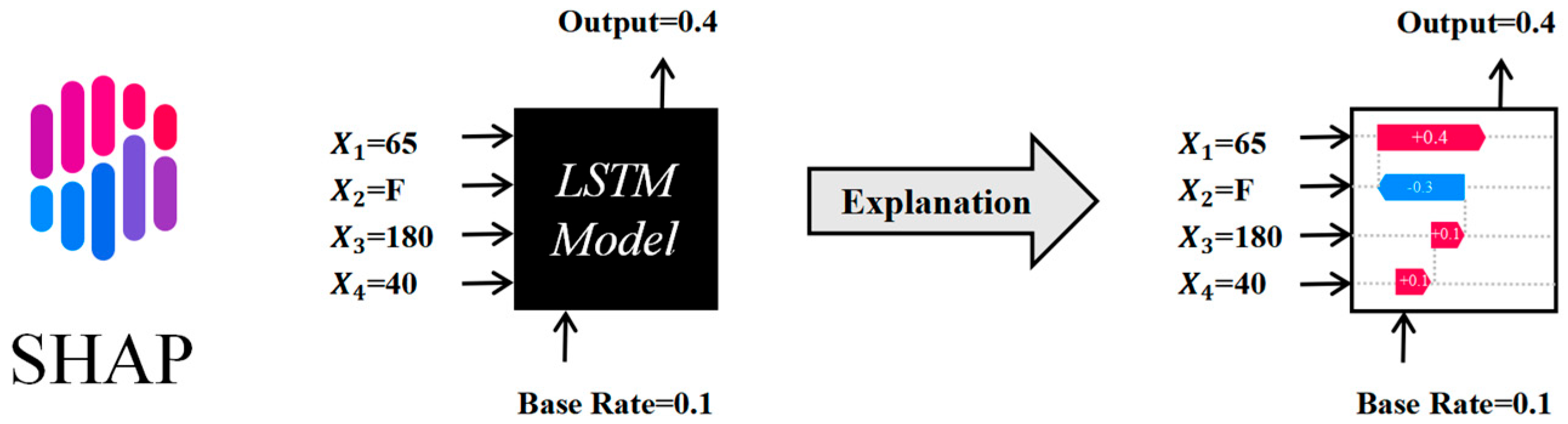
where $M$ is the number of features, $\mathcal{F}=\{1,2,\dots ,M\}$ and $v\left(S\right)$ denotes the expected model output when only features in $S$ are observed and the remaining features are integrated out using conditional expectations. The resulting SHAP values provide an interpretable decomposition of the prediction (Figure 2). In this study, an LSTM model is used as the base learner for SHAP analysis to identify model-based feature-importance patterns that inform subsequent forecasting and heterogeneity analysis [30].

2.3. LSTM–Transformer Model

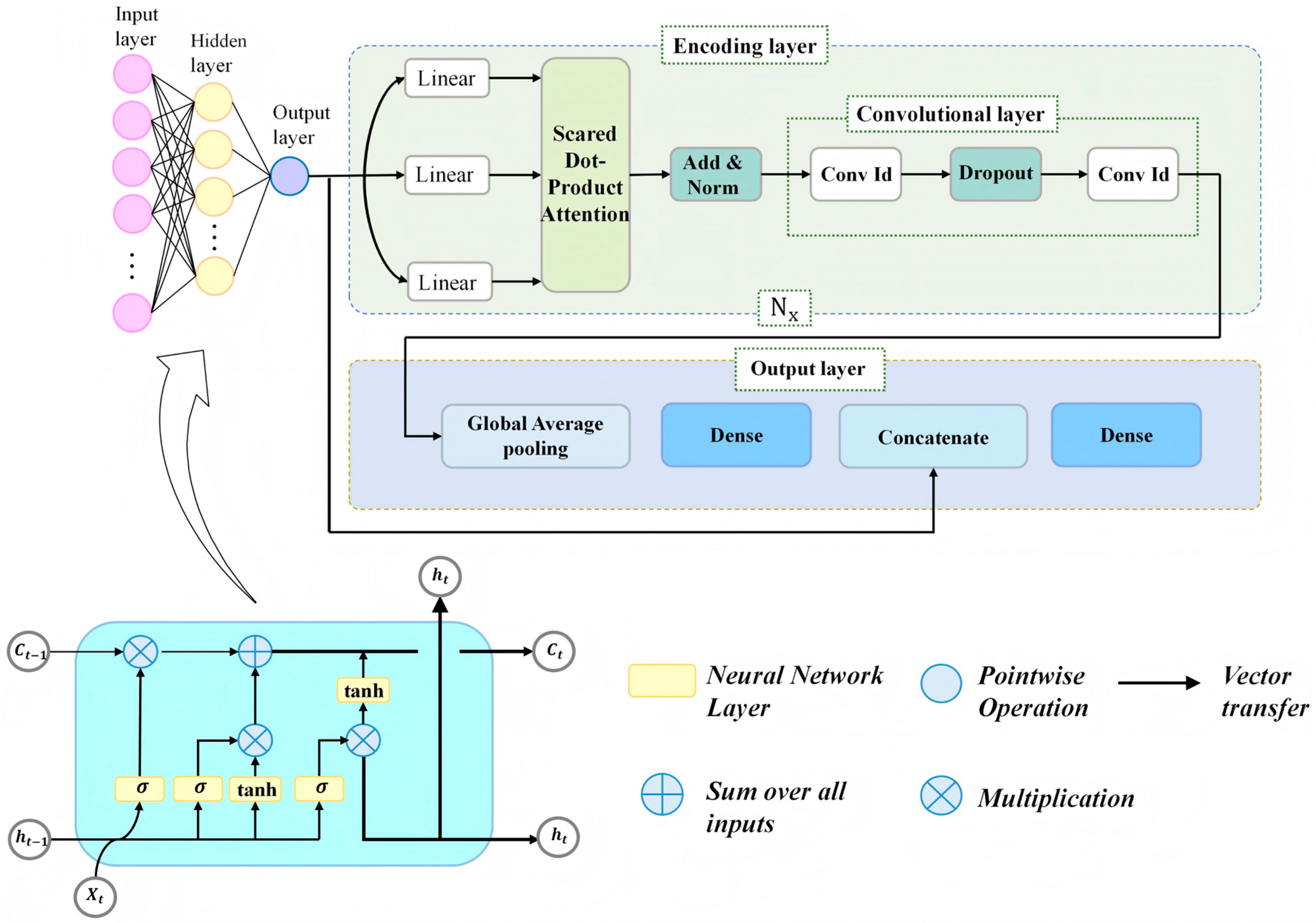
To capture heterogeneous temporal patterns in provincial carbon emissions, we build a hybrid LSTM–Transformer forecasting model with two complementary branches. The LSTM branch captures short-term memory effects and local temporal dynamics, while the Transformer encoder models longer-range cross-period dependencies through self-attention. The two feature streams are concatenated at the output stage to generate the final forecast. The overall architecture is shown in Figure 3 [31].

2.3.1. Input and Output Definition

Let the driver vector at time $t$ be $x_t\in {\mathbb{R}}^M$ and carbon emissions be $y_t\in \mathbb{R}$. Using a sliding window of length $L$, the input sequence is [32]

$$X_t=[x_{t-L+1},x_{t-L+2},\dots ,x_t]\in {\mathbb{R}}^{L\times M},$$

(5)

and the target is carbon emissions $H$ steps ahead, $y_{t+H}$. In the empirical experiments, the base model is trained for one-step-ahead prediction (H = 1). Multi-step projections are produced recursively by feeding the predicted emission at step t + 1 back into the input for subsequent steps.

2.3.2. LSTM Module

Carbon emissions and their drivers often exhibit temporal dependence and lagged effects. We therefore include an LSTM branch that uses gating to control information flow and produce a stable temporal representation [33]. For the $k$-th step in the window, the input is $x_k$ (corresponding to $x_{t-L+k}$). The LSTM updates are

$$\begin{gathered} i_k=\sigma (W_i{x}_k+U_i{h}_{k-1}+b_i), \\ {f}_k=\sigma (W_f{x}_k+U_f{h}_{k-1}+b_f), \\ {o}_k=\sigma (W_o{x}_k+U_o{h}_{k-1}+b_o), \\ {\tilde{c}}_k=\mathrm{t}\mathrm{a}\mathrm{n}\mathrm{h}(W_c{x}_k+U_c{h}_{k-1}+b_c), \\ {c}_k=f_k\odot c_{k-1}+i_k\odot {\tilde{c}}_k, \\ {h}_k=o_k\odot \mathrm{t}\mathrm{a}\mathrm{n}\mathrm{h}\left(c_k\right), \end{gathered}$$

(6)

where $\sigma (\cdot )$ is the sigmoid function and $\odot$ denotes element-wise multiplication. $h_k$ and $c_k$ are the hidden state and memory state at step $k$; $i_k$, $f_k$, and $o_k$ are the input, forget, and output gates. After $L$ recurrent steps, we take the final hidden state $h_L\in {\mathbb{R}}^{d_h}$ as the LSTM feature representation of the historical window.

In the integrated framework, this LSTM representation primarily serves to encode short-term memory and local temporal continuity in the emission sequence, providing a stable sequential backbone for the downstream fusion.

2.3.3. Transformer Module

In a complex emission system, interactions can span across time steps, and variables may be coupled through nonlinear relationships [34]. To model these cross-time and cross-variable dependencies, we introduce a Transformer encoder. The module first projects $X_t$ into a shared feature space and adds positional encoding to preserve time order

$$E_0=PE(X_t{W}_e+b_e),$$

(7)

where $W_e\in {\mathbb{R}}^{M\times d}$ and $b_e\in {\mathbb{R}}^d$ are learnable parameters and $E_0\in {\mathbb{R}}^{L\times d}$ is the initial input to the encoder. Positional encoding $PE(\cdot )$ provides temporal information that self-attention does not carry by default.

1.

Self-attention: scaled dot-product attention

At the $n$-th encoder layer, self-attention evaluates the relevance between a given time step and all other steps in the window, then aggregates information accordingly [34]. For the layer input $E_{n-1}\in {\mathbb{R}}^{L\times d}$, we form queries, keys, and values via linear projections:

$$Q=E_{n-1}{W}_Q,K=E_{n-1}{W}_K,V=E_{n-1}{W}_V,$$

(8)

where $W_Q,W_K,W_V\in {\mathbb{R}}^{d\times d_k}$ are learnable matrices and $d_k$ is the key/query dimension for a single head. Attention weights are computed using scaled dot products and applied to $V$:

$$Att(Q,K,V)=\mathrm{s}\mathrm{o}\mathrm{f}\mathrm{t}\mathrm{m}\mathrm{a}\mathrm{x}\left({\displaystyle \frac{Q{K}^{\mathrm{\top }}}{d_k}}\right)V,$$

(9)

where $Q{K}^{\mathrm{\top }}/d_k$ measures similarity between representations at different time steps and $\mathrm{s}\mathrm{o}\mathrm{f}\mathrm{t}\mathrm{m}\mathrm{a}\mathrm{x}(\cdot )$ normalizes these scores into weights so the model can focus on the most informative history. The scaling by $d_k$ helps prevent large dot products from saturating the softmax and destabilizing training.

To improve expressiveness, multi-head attention computes this operation in parallel across $h$ heads, each attending to a different subspace, then concatenates head outputs followed by a linear projection, denoted as $MHA(\cdot )$ [35]. We apply a residual connection and layer normalization:

$$E_n=\mathrm{L}\mathrm{a}\mathrm{y}\mathrm{e}\mathrm{r}\mathrm{N}\mathrm{o}\mathrm{r}\mathrm{m}\left(E_{n-1}+MHA\left(E_{n-1}\right)\right).$$

(10)

The residual pathway preserves the original representation, while layer normalization stabilizes training and supports better generalization. The resulting $E_n$ is passed to the convolutional feed-forward block.

2.

Convolutional feed-forward block

Standard Transformers use a position-wise feed-forward network after attention. Given the presence of local fluctuations and stage-like patterns in emission series [35], we implement this component using 1D convolutions to enhance local feature extraction:

$$FF{N}_{conv}\left(E_n\right)={\mathrm{C}\mathrm{o}\mathrm{n}\mathrm{v}1\mathrm{d}}_2\hspace{0.17em}\left(\mathrm{D}\mathrm{r}\mathrm{o}\mathrm{p}\mathrm{o}\mathrm{u}\mathrm{t}\left(\varphi \right({\mathrm{C}\mathrm{o}\mathrm{n}\mathrm{v}1\mathrm{d}}_1\left(E_n\right)\left)\right)\right),$$

(11)

where $\varphi (\cdot )$ is the activation function (ReLU in this study) and Dropout is used to mitigate overfitting. We again apply a residual connection and layer normalization:

$$E_n=\mathrm{L}\mathrm{a}\mathrm{y}\mathrm{e}\mathrm{r}\mathrm{N}\mathrm{o}\mathrm{r}\mathrm{m}\hspace{0.17em}\left(E_n+FF{N}_{conv}\left(E_n\right)\right).$$

(12)

This “attention with convolutional feed-forward” encoder block is repeated $N_x$ times, yielding the final Transformer sequence representation:

$$Z=E_{N_x}\in {\mathbb{R}}^{L\times d}.$$

(13)

Each time step in $Z$ integrates information from the entire window, capturing cross-period dependencies and variable interactions [36].

Compared with the recurrent branch, the Transformer branch mainly adds the ability to model long-range cross-period dependencies and global interactions within the input window, which may be difficult to capture fully through sequential recursion alone.

2.3.4. Dual-Branch Fusion

Since the Transformer output $Z$ remains a sequence, we aggregate it over the time dimension using global average pooling:

$$z={\displaystyle \frac{1}{L}}\sum _{k=1}^L{Z}_k\in {\mathbb{R}}^d.$$

(14)

This summarizes the window-level information and reduces sensitivity to noise at individual time steps. A fully connected layer then produces a regression-friendly representation:

$$z^{\prime }=\psi (W_{z}z+b_z),$$

(15)

where $\psi (\cdot )$ is a nonlinear activation function. We concatenate the LSTM representation $h_L$ and the Transformer representation $z^{\prime }$ to form the fused vector:

$$u=[h_L;z^{\prime }]\in {\mathbb{R}}^{d_h+d}.$$

(16)

Finally, the output layer generates the forecast:

$$y_{t+H}=W_{o}u+b_o.$$

(17)

This fusion explicitly combines the LSTM’s strength in modeling short-term memory and local temporal dynamics with the Transformer’s advantage in capturing long-range dependencies, thereby providing a functionally complementary representation for carbon emission forecasting.

2.4. SSA-Based Optimization

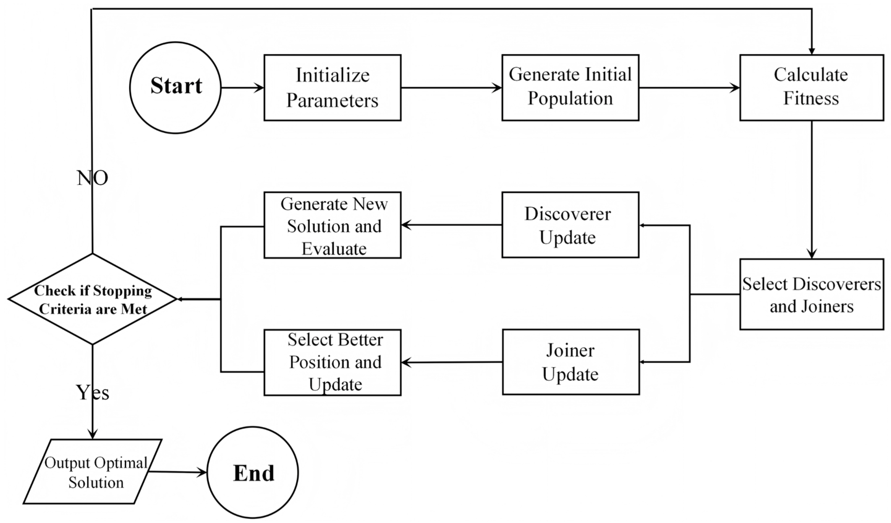
In the proposed framework, SSA is used as an adaptive hyperparameter optimization strategy for the LSTM–Transformer model rather than as a forecasting module. It searches the hyperparameter space (e.g., window length, hidden dimension, attention heads, dropout, and learning rate) and reduces the uncertainty and computational burden associated with manual tuning or exhaustive search. By balancing exploration and exploitation, SSA improves search efficiency, convergence stability, and generalization performance [37]. The workflow is illustrated in Figure 4.

SSA treats each candidate solution as a “sparrow,” where the position vector represents a specific hyperparameter configuration. Let the search space have dimension $D$ and the population size be $N$. At iteration $t$, the position of the $i$-th sparrow is

$$x_i^t=\left(x_{i,1}^t,x_{i,2}^t,\dots ,x_{i,D}^t\right),$$

(18)

where each component corresponds to one hyperparameter. We use validation error as the fitness function. For the $d$-th dimension, the update rule is [37]

$$x_{i,d}^{t+1}=x_{i,d}^t+r\left(x_{best,d}^t−x_{i,d}^t\right),$$

(19)

where $x_{best,d}^t$ is the $d$-th component of the global best solution at iteration $t$ and $r\in (0,1)$ is a random coefficient. The global best solution is updated whenever a better fitness value is found, and the process continues until the maximum number of iterations is reached or the fitness converges. Within the integrated framework, SSA contributes to optimization efficiency, while the LSTM–Transformer architecture performs temporal representation learning and forecasting.

Therefore, within the integrated framework, SSA contributes by improving hyperparameter search efficiency and optimization robustness, while the LSTM–Transformer architecture remains responsible for temporal representation learning and forecasting.

3. Carbon Emission Driving Factors Identification Results

3.1. SHAP-Based Driver Importance Results

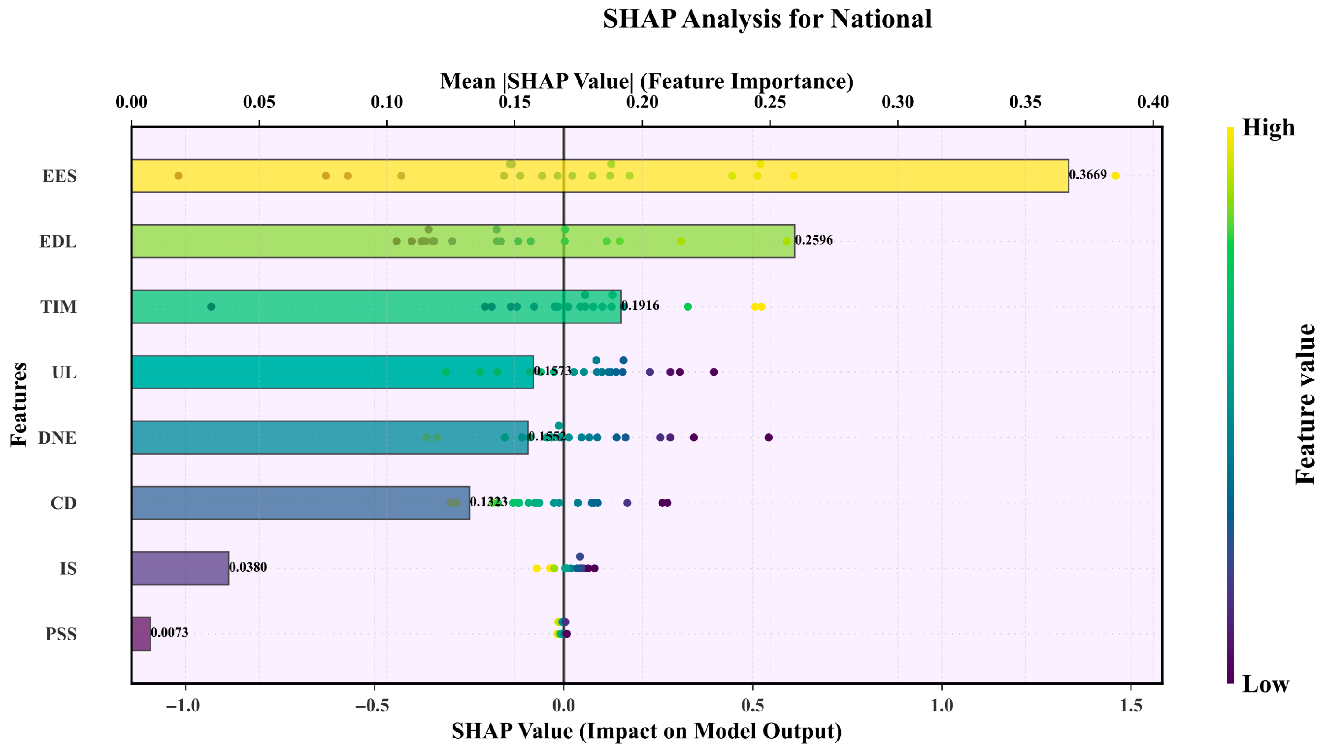
Based on the national SHAP results (see Figure 5), the most influential features in the model’s carbon emission predictions are, in descending order, the energy-consumption structure (EES, mean SHAP value 0.367), the level of economic development (EDL, 0.260), and technological innovation (TIM, 0.192). EES shows the largest and most consistent contribution pattern. Its feature values (blue to yellow) align monotonically with SHAP values (negative to positive), indicating that a higher share of carbon-intensive energy is associated with higher predicted emissions under the fitted model. The contribution pattern of EDL is nonlinear. At lower development levels, the sign of the SHAP contribution varies across observations, while at higher levels it is predominantly positive, suggesting that economic development is strongly aligned with higher predicted emission levels in the current sample period [38]. TIM exhibits a predominantly negative contribution pattern, with observations at higher innovation levels concentrated on the negative SHAP side, indicating an association between stronger innovation capacity and lower predicted emissions.

Other factors, including urbanization (UL), non-energy sector emission intensity (DNE), and carbon emission density (CD), show moderate contributions, whereas industrial structure (IS) and policy/social support (PSS) have relatively smaller direct contributions in the current predictive model. These SHAP-based rankings should be interpreted as model-based feature importance rather than causal effects, since the analysis is observational and the features may be correlated. From a policy perspective, the results highlight predictive patterns that are consistent with prioritizing cleaner energy structures and strengthening innovation-related capacity in differentiated mitigation planning.

3.2. Heterogeneity Analysis

3.2.1. Rules for Regional Division

China’s provinces differ markedly in development stage, resource endowments, and industrial structure, so a single model can miss region-specific emission dynamics. We therefore conduct a regional heterogeneity analysis. Following the classification approach and the IPCC-style grouping used in related work, provinces (excluding Hong Kong, Macao, Taiwan and Tibet) are grouped into three categories based on development stage, energy intensity, and industrialization level: Developed Provinces, Rapidly Developing Provinces, and Developing Provinces [39].

(1)

Developed Provinces: regions with advanced economic development and a clear shift from heavy industry toward high tech and services. These provinces typically exhibit higher energy efficiency and stronger innovation capacity, with emissions often stabilizing or trending downward.

(2)

Rapidly Developing Provinces: regions in the middle-to-late stage of industrialization, with strong growth momentum and fast urbanization. They usually have a large manufacturing base and high energy demand, making them central to balancing growth and emission pressure in the near term.

(3)

Developing Provinces: regions with later economic take-off, still driven by resources or in an accelerated industrialization phase. They tend to rely on conventional energy supply or energy-intensive industries. Current emissions may be lower, but the growth potential is substantial as infrastructure investment and industrial relocation continue.

The classification results are reported in

Table 2. Regional heterogeneity classification by province.

Classification	Provincial-Level Region
Developed Provinces	Beijing (BJ), Shanghai (SH), Tianjin (TJ), Jiangsu (JS), Zhejiang (ZJ), Guangdong (GD), Fujian (FJ)
Rapidly Developing Provinces	Shandong (SD), Hebei (HEB), Hubei (HB), Hunan (HN), Henan (HEN), Sichuan (SC), Anhui (AH), Jiangxi (JX), Shaanxi (SAX), Liaoning (LN), Jilin (JL), Heilongjiang (HL)
Developing Provinces	Chongqing (CQ), Hainan (HAN), Shanxi (SX), Inner Mongolia (NAM), Guangxi (GX), Guizhou (GZ), Yunnan (YN), Gansu (GS), Qinghai (QH), Ningxia (NX), Xinjiang (XJ)

.

3.2.2. Heterogeneity Test Results

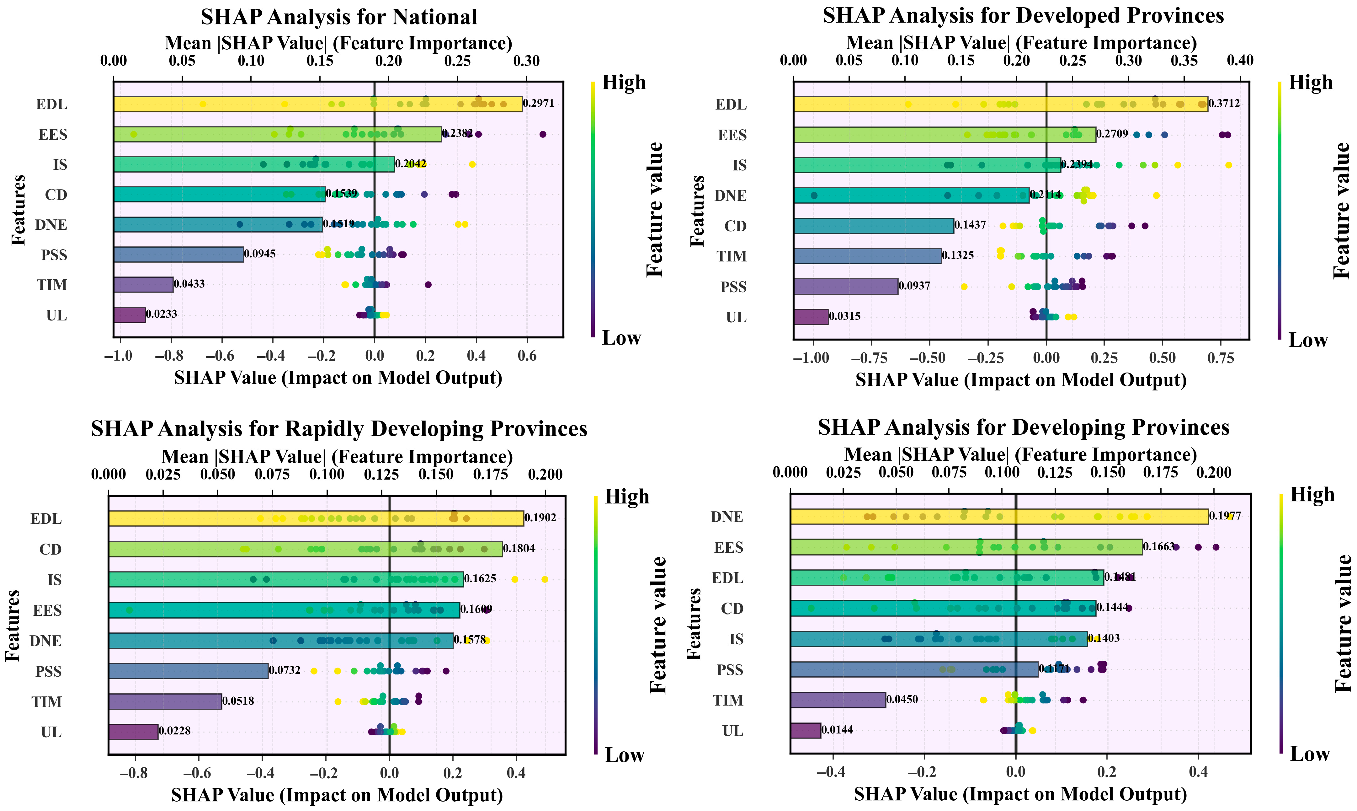
We then conduct region-specific SHAP analysis (see Figure 6). Comparing the regional SHAP plots indicates clear stage-dependent heterogeneity in the model-based importance patterns across province groups. At the national level, EES (mean SHAP value 0.35) remains the most influential feature in the model’s predictions, with higher EES values associated with higher predicted emissions. EDL (0.29) and TIM (0.29) follow, and TIM exhibits a predominantly negative contribution pattern overall.

The SHAP contribution patterns differ across regions. In developed provinces, TIM (mean SHAP value about 0.59) becomes the most influential feature, and higher TIM values are concentrated on the negative SHAP side, indicating that higher innovation levels are associated with lower predicted emissions under the fitted model. In rapidly developing provinces, EES (mean SHAP value about 0.36) again shows the largest positive contribution, while TIM displays a relatively weak positive contribution pattern [40]. This pattern is consistent with a context in which efficiency-related improvements may coincide with expanding energy demand during industrialization, although the SHAP results themselves should be interpreted as predictive associations rather than causal effects. In developing provinces, the mean SHAP values of the eight features are identical (all 0.254), indicating a more even distribution of feature contributions across economic, energy, technology, and urbanization-related variables, without a single dominant feature in the predictive model.

Overall, these results suggest that the model-based driver importance structure varies systematically with development stage. This heterogeneity implies that interpreting driver rankings or designing policy priorities using a single national-average pattern may be insufficient, and that region-specific evidence can provide a more informative basis for differentiated mitigation planning.

3.2.3. Statistical Test of Heterogeneity

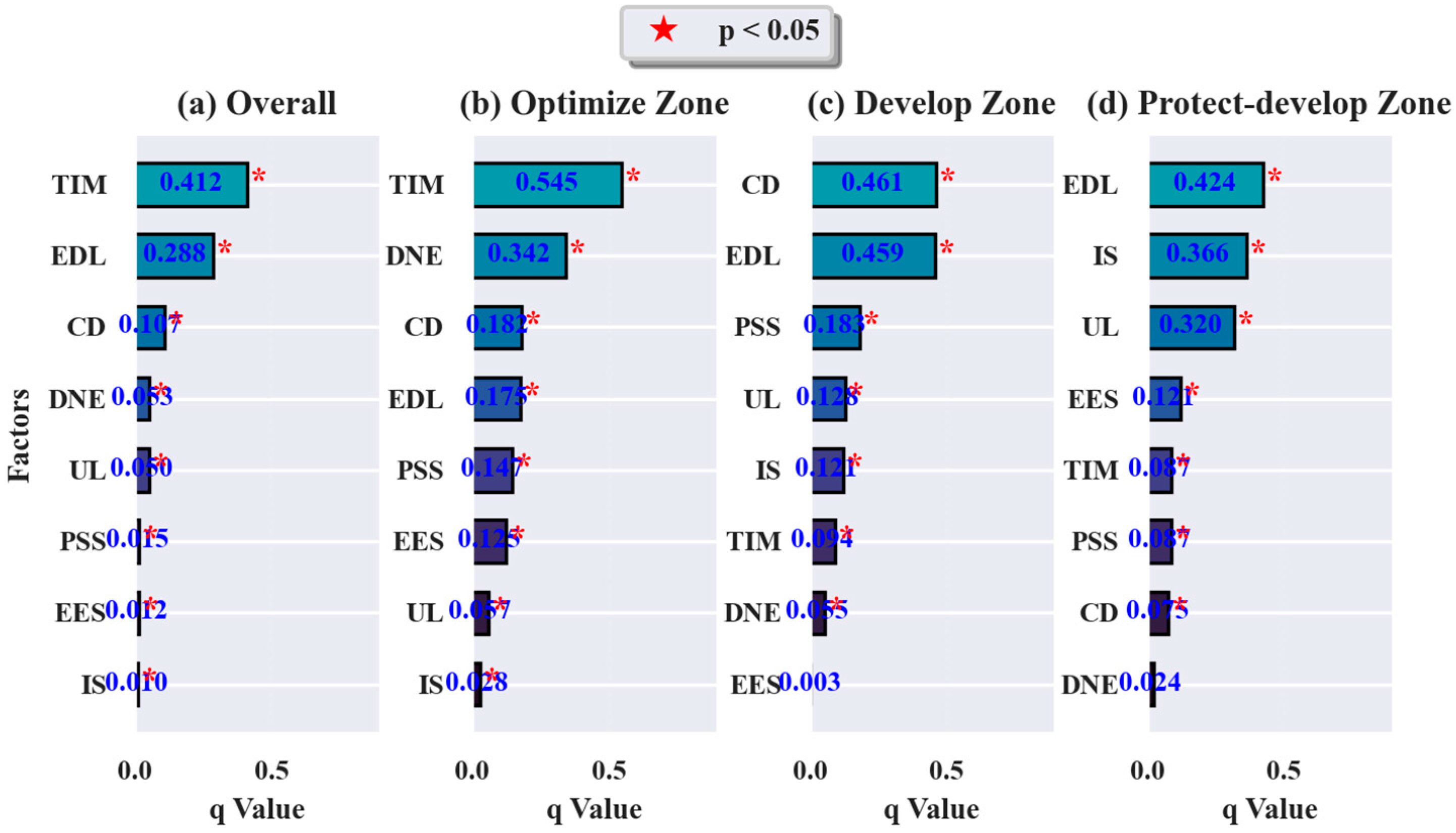
To test the regional heterogeneity of driver effects more rigorously, we apply the q-statistic from the geographic detector framework and assess significance using a Monte Carlo permutation test. Figure 7 reports the q values and corresponding p values for each factor across regions (Overall, Optimize Zone, Develop Zone, and Protect–Develop Zone).

The q-statistic measures how strongly a driver explains spatial differentiation in the driver effect, using SHAP values as the outcome of interest [41]. It is defined as

$$q=1-{\displaystyle \frac{{\sum }_{h=1}^L{N}_h{\sigma }_h^2}{N{\sigma }^2}},$$

(20)

where $N_h$ and ${\sigma }_h^2$ are the sample size and SHAP-value variance within stratum $h$ (defined by the driver $X$ or by regional grouping), and $N$ and ${\sigma }^2$ are the total sample size and overall SHAP-value variance, $q\in [0,1]$. Larger values indicate stronger spatial heterogeneity, meaning the driver effect varies more across provinces.

We evaluate statistical significance using a Monte Carlo permutation test. Under the null hypothesis that the driver has no influence on the spatial distribution of SHAP values, we randomly permute the pairing between driver values and provincial regions, recompute q for the shuffled data, and repeat this procedure 1000 times to obtain an empirical null distribution of q. The p value is defined as the proportion of simulated q values that are greater than or equal to the observed q. If p < 0.05, we reject the null hypothesis and conclude that the driver effect exhibits significant spatial heterogeneity.

At the national level, the q values for EDL, TIM, and UL are generally low and not statistically significant, suggesting relatively similar SHAP contribution patterns across provinces in the aggregate. The regional results, however, show clearer heterogeneity across zone groupings. In the Optimize Zone (dominated by developed regions such as Beijing and Shanghai), the q values for economic development and technological innovation are higher and statistically significant, indicating greater cross-province variation in their SHAP contributions within this zone. In the Develop Zone (dominated by industrial provinces such as Shandong and Henan), the q values for energy-consumption structure and industrial structure are relatively higher, suggesting more pronounced spatial differentiation in the corresponding SHAP contribution patterns. In the Protect–Develop Zone (often less developed or ecologically constrained western provinces), urbanization and policy/social support show statistically significant q values, indicating stronger heterogeneity in their SHAP contributions across provinces within this zone. These results provide quantitative evidence that feature-importance patterns are region-dependent and should be interpreted cautiously, with attention to development stage and regional context.

3.3. Comparison with Existing Studies

The results of this study can be further interpreted by comparing them with existing research on carbon emission forecasting and driver analysis. In terms of overall importance patterns, the national SHAP results are broadly aligned with the literature that emphasizes energy structure and economic development as prominent correlates of emission variation. In our model-based decomposition, the energy-consumption structure shows the largest contribution to predicted emissions, while the level of economic development is associated with higher predicted emission levels in many observations at the current stage [19,20]. In addition, the SHAP results provide a nonlinear view of these associations. For economic development, the sign and magnitude of contributions vary across the value range and become more consistently positive at higher levels, illustrating how contribution strength changes within the sample distribution compared with linear or average-effect summaries [21,22].

Technological innovation provides another point of comparison. Many previous studies report a negative association between innovation-related indicators and emissions, although the reported patterns differ across datasets, regions, and modeling approaches. The national SHAP results in this study show that higher TIM values are more often associated with negative SHAP contributions, indicating lower predicted emissions under the fitted model [23]. The regional analysis further suggests that this contribution pattern is not uniform across development stages. In developed provinces, TIM exhibits a more consistently negative contribution pattern, whereas in rapidly developing provinces the contribution pattern is weaker and may appear positive in some cases under strong growth and energy-demand conditions. This contrast provides a model-based perspective that is consistent with the mixed evidence reported in prior studies, and it suggests that development stage, industrial structure, and energy dependence should be considered when interpreting feature-importance rankings [25,26]. These results should be interpreted cautiously, as SHAP values reflect predictive contributions within the model and do not establish causal effects.

Compared with studies that focus on national averages or broad regional comparisons, the heterogeneity analysis in this paper provides a more explicit characterization of stage-dependent feature-importance structures. The combination of region-specific SHAP analysis and statistical heterogeneity testing indicates that the relative contribution patterns of key features differ across province groups [27]. Developed provinces show a stronger negative contribution pattern for innovation-related indicators, rapidly developing provinces exhibit a more prominent contribution from energy-structure variables alongside industrialization-related factors, and developing provinces display a more balanced distribution of contributions across multiple features. This comparative evidence extends the existing literature by linking machine learning-based contribution decomposition with interpretable regional differentiation, which is informative for context-aware and region-specific mitigation planning [29].

4. SSA–LSTM–Transformer Forecasting Results

4.1. Model Evaluation

To assess the robustness and performance of the SSA–LSTM–Transformer model, we use two complementary evaluation strategies. Internally, we run ablation tests by removing and recombining the SSA, LSTM, and Transformer components to quantify each module’s marginal contribution to accuracy. Externally, we benchmark the proposed model against a set of widely used carbon emission forecasting approaches. Performance is measured with five statistical metrics. To reduce the influence of units and scale, the metrics are normalized/standardized as needed. The metrics are defined as

$$\begin{gathered} R^2=1-{\displaystyle \frac{{\sum }_{i=1}^n(y_i-{\widehat{y}}_i{)}^2}{{\sum }_{i=1}^n(y_i-\overline{y}{)}^2}}, \\ NRMSE={\displaystyle \frac{RMSE}{y_{\mathrm{m}\mathrm{a}\mathrm{x}}-y_{\mathrm{m}\mathrm{i}\mathrm{n}}}}, \\ CVRMSE={\displaystyle \frac{RMSE}{{\displaystyle \overline{y}}}}\times 100\mathrm{\%}, \\ sMAPE={\displaystyle \frac{100\mathrm{\%}}{n}}{\sum }_{i=1}^n{\displaystyle \frac{2\mid y_i-{\widehat{y}}_i\mid }{ϵ+\mid y_i\mid +\mid {\widehat{y}}_i\mid }}, \\ NMAE={\displaystyle \frac{MAE}{y_{\mathrm{m}\mathrm{a}\mathrm{x}}-y_{\mathrm{m}\mathrm{i}\mathrm{n}}}} \end{gathered}$$

(21)

where $y_i$ is the observed value, ${\widehat{y}}_i$ is the prediction, $n$ is the number of samples, $y_{\mathrm{m}\mathrm{a}\mathrm{x}}$ and $y_{\mathrm{m}\mathrm{i}\mathrm{n}}$ are the maximum and minimum of the observed values, and ${\displaystyle \overline{y}}$ is the mean. We set $ϵ={10}^{-8}$. A larger $R^2$ (closer to 1) indicates better fit. Smaller NRMSE and NMAE indicate lower relative error and are convenient for cross-region comparison; NRMSE is more sensitive to large fluctuations and is useful for assessing stability. CVRMSE is commonly used in energy-related evaluation, where lower is better. sMAPE is more stable when true values are small and preserves symmetry in percentage errors, improving comparability across provinces with very different emission levels.

We use provincial panel data from 2005–2022 and apply a chronological (time-ordered) split to construct the training, validation, and test sets, avoiding random partitioning and thus reducing the risk of temporal information leakage. Specifically, 2005–2017 is used for training (390 province–year observations) for parameter learning, 2018–2020 is used for validation (90 observations) for SSA-based hyperparameter optimization and model selection, and 2021–2022 is reserved as a fully held-out test period (60 observations) for final performance evaluation only. The training set is used for parameter learning, the validation set is used by SSA for hyperparameter optimization and model selection, and the test set is kept fully held out for final performance evaluation only. This design improves the transparency of model evaluation and provides a stricter assessment of out-of-sample forecasting ability on unseen periods.

To reduce overfitting risk, we separate hyperparameter tuning from final testing and use the validation set as the only basis for SSA-based search decisions. In addition, the model architecture includes regularization mechanisms (e.g., dropout and layer normalization), and the comparison on the held-out test set is used to verify whether performance gains generalize beyond the training and validation periods. Given the limited time span of annual data, we interpret the results with caution and emphasize out-of-sample performance rather than in-sample fit.

4.1.1. Iterative Curve of the SSA Model

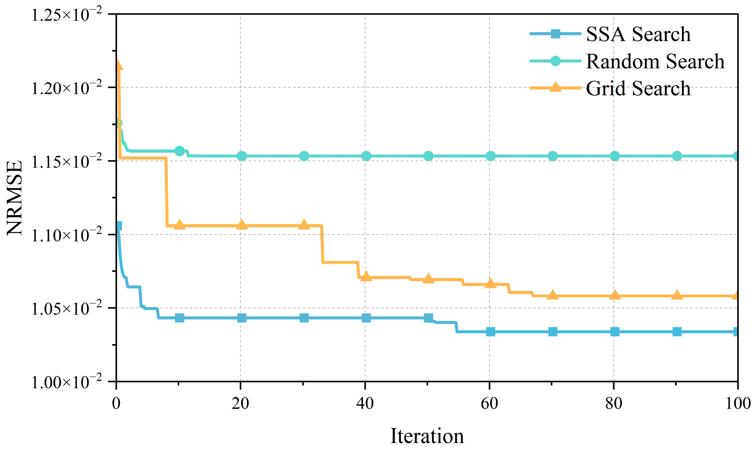
To evaluate the optimization efficiency of SSA, we benchmark its search trajectory and final performance against two widely used baselines, grid search and random search, within the same hyperparameter search space. In SSA, the population size is set to N = 50, and the maximum number of iterations is 100. The optimization objective is the validation NRMSE, and we record the best-so-far NRMSE at each iteration to summarize search progress. The tuned hyperparameters include the embedding dimension, number of attention heads, number of Transformer layers, LSTM hidden size, number of LSTM layers, dropout rate, learning rate, and batch size. For comparability, grid search and random search are executed over the same parameter ranges. Grid search evaluates a predefined discrete grid, while random search samples candidate configurations from the same ranges under an equivalent evaluation budget. The final forecasting performance under each search strategy is reported in

Table 3. Performance comparison of SSA search and other search methods.

Models	NRMSE	R2	NMAE	sMAPE	CVRMSE
Our Work	0.0192	0.9911	0.0127	0.0492	0.0611
Grid Search	0.0375	0.9663	0.0212	0.1563	0.0763
Random Search	0.0451	0.9532	0.0351	0.2365	0.0845

, and the best-so-far validation NRMSE curves are shown in Figure 8.

Figure 8 indicates that SSA improves validation performance rapidly in the initial iterations and maintains the lowest best-so-far NRMSE across the search process. After the early decrease, the SSA curve exhibits a gradual refinement pattern, with smaller yet persistent gains before reaching a stable plateau. The random-search curve shows an early improvement followed by diminishing returns, reflecting the fact that random sampling can quickly find reasonable configurations but becomes less efficient at locating near-optimal settings as the budget increases. The grid-search curve decreases in a stepwise manner and remains above the SSA curve over most iterations, suggesting lower search efficiency under the same search-space constraints. Consistent with these trajectory patterns, Table 3 shows that the SSA-optimized model achieves the best overall forecasting accuracy among the compared strategies, supporting the use of SSA for efficient hyperparameter optimization in the proposed LSTM–Transformer framework.

4.1.2. Ablation Study

To clarify the role of each module, we define S (SSA optimization), L (LSTM branch), and T (Transformer encoder). Results are reported in

Table 4. Ablation Results.

Metrics	Our Work	T + S	L + S	L + T	T	L
NRMSE	0.0192	0.0401	0.0392	0.0344	0.0503	0.0289
Rank	1	5	4	3	6	2
R2	0.9911	0.9599	0.9618	0.9662	0.9636	0.9813
Rank	1	6	5	3	4	2
NMAE	0.0127	0.0227	0.0224	0.0219	0.0288	0.0222
Rank	1	5	4	2	6	3
sMAPE	0.0492	0.269	0.0846	0.1046	0.1007	0.9390
Rank	1	5	2	4	3	6
CVRMSE	0.0611	0.0813	0.1363	0.1321	0.1479	0.9190
Rank	1	2	4	3	5	6
Total	5	23	19	15	24	19

.

Our work configuration ranks first on every metric. The Transformer branch captures global dependencies more effectively than a standalone LSTM, but without the LSTM’s recurrent memory, $R^2$ drops slightly. Adding SSA improves accuracy by about 52% relative to the non-optimized version, highlighting the value of swarm-based hyperparameter search.

4.1.3. Benchmark Comparison

To evaluate real-world performance, we compare SSA–LSTM–Transformer against eight commonly used baselines, covering neural networks (BP, ANN, MLP) [17], tree-based models (GBDT, XGBoost, LightGBM) [42], and classic machine learning models (SVM, RF) [43]. All baselines are trained and tested on the same data and evaluated using the same metrics. The best hyperparameter settings are listed in Appendix A (

Table A1. The parameters of the algorithm used in this study.

Model	Parameter (Optimization Value)
LSTM	EmbDim = 122; Heads = 2; TransLayers = 2; LSTM Hidden = 51; LSTM Layers = 1; Dropout = 0.1375; LR = 0.006785; Batch = 11
Transformer	PosEnc Params = 12,200; InputProj = 1832 (12->122); Encoder Params = 305,592 (2 layers); Attention Params = 7565
LSTM	Proj = 663 (12->51); Layer Params = 21,216 (1 layer); Norm Params = 102
BP	InputDim = 40; Hidden = [128,64,32]; LR = 0.001; Dropout = 0.2; L2 = 0.0001
ANN	InputDim = 40; Total Params = 54,721
MLP	InputDim = 40
GBDT	InputDim = 40
XGBoost	Trees = 100; MaxDepth = 6; LR = 0.1
LightGBM	Trees = 100; MaxDepth = 6; LR = 0.1; RandomState = 42
SVM	Kernel = rbf; C = 1; Epsilon = 0.1
RF	Trees = 100; MaxDepth = 10
SSA	Population size N = 50; Max iterations T = 100; Fitness = validation NRMSE; Search space = {EmbDim, Heads, TransLayers, LSTM Hidden, LSTM Layers, Dropout, LR, Batch}

). Summary results are shown in

Table 5. Benchmark results.

Metrics	Our Work	BP	ANN	MLP	GBDT	XGBoost	LightGBM	SVM	RF
NRMSE	0.0192	0.1062	0.0453	0.0574	0.1119	0.1217	0.1165	0.1340	0.1242
Rank	1	4	2	3	5	7	6	9	8
R2	0.9911	0.8008	0.9638	0.9417	0.7788	0.7295	0.7521	0.6725	0.7185
Rank	1	4	2	3	5	7	6	9	8
NMAE	0.0127	0.0866	0.0316	0.0463	0.0797	0.0802	0.0814	0.0948	0.0843
Rank	1	8	2	3	4	5	6	9	7
sMAPE	0.0492	0.3871	0.1186	0.1808	0.2641	0.2464	0.2572	0.3039	0.2679
Rank	1	9	2	3	6	4	5	8	7
CVRMSE	0.0611	0.3123	0.1331	0.1690	0.3291	0.3605	0.3452	0.3967	0.3678
Rank	1	4	2	3	5	7	6	9	8
Total	5	29	10	15	25	30	29	44	38

.

Overall, SSA–LSTM–Transformer delivers the best performance on the core metrics (NRMSE, $R^2$, NMAE) and ranks first overall. For example, $R^2$ reaches 0.9911, compared with 0.6725 for SVM, a gap of 0.3186. NRMSE is 0.0192, which is 85.7% lower than the worst-performing model. By model family, ANN and MLP consistently rank near the top with the proposed model, each keeping the total score below 15. Tree-based methods and traditional machine learning models (GBDT, XGB, LGBM, RF, SVM) generally score above 25, suggesting that deep architectures provide more stable accuracy for this task. Under extreme-error cases, sMAPE is 0.0492 for the proposed model versus 0.3871 for BP, a roughly 7.8 times reduction, indicating better control of cross-provincial volatility. In terms of fit, deep-learning models (the proposed model, LSTM, Transformer) stay above 0.96, while conventional methods such as SVM and RF are mostly below 0.75. This aligns with the advantage of deep networks in capturing nonlinear fluctuations and long-range dependence in emission series.

4.2. Forecast Results

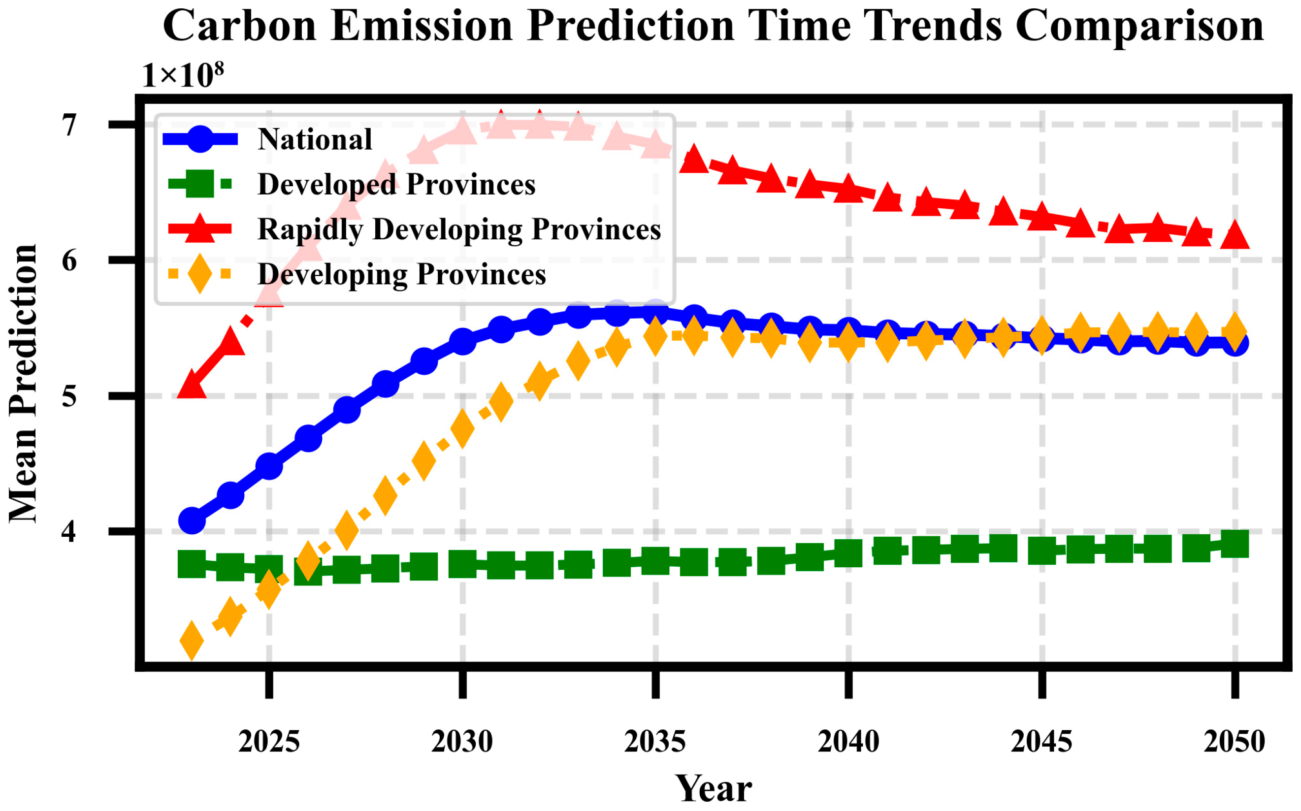
Figure 9 reports the mean forecast trajectories together with uncertainty bands (shown as prediction intervals) for the national total and the three provincial development-stage groups. The central trajectories indicate distinct emission paths across provinces at different development stages. In the early horizon (2025–2035), rapidly developing provinces show a slightly steeper growth slope, consistent with rising emissions pressure from industrialization and urbanization. Developed provinces exhibit a flatter curve, suggesting a more stable industrial structure and gradually strengthening technology-driven mitigation. Developing provinces start close to the national mean but follow a different growth rhythm in the mid-horizon. Despite these early differences, the four mean curves converge more noticeably in the later period, approaching similar emission levels by 2050 under the model assumptions.

The uncertainty bands widen with the forecast horizon, indicating increasing uncertainty as recursive forecasting steps accumulate. In a recursive multi-step setting, the forecast at step $h$ depends on outputs predicted at earlier steps, so prediction errors can propagate forward and accumulate over the horizon. Conceptually, the $h$-step-ahead forecast error contains both the new one-step error at step $h$ and the compounded influence of errors generated in the previous recursive steps. Under simplifying assumptions where one-step errors are approximately unbiased and weakly correlated, the uncertainty of $h$-step forecasts is expected to increase with the horizon, which provides a direct explanation for the widening prediction intervals in Figure 9 as the projection moves toward 2050. In practice, nonlinear dynamics and changing driver conditions may further amplify or dampen this accumulation, so uncertainty growth is not necessarily linear, yet it is expected to be monotonic in long-horizon recursive projections. This error-propagation property reinforces the interpretation that later-horizon results provide more reliable information on relative trajectories and convergence tendencies than on precise point levels. This pattern is expected in medium- to long-term projections and suggests that the later-period convergence should be interpreted as a trend tendency in the mean forecast rather than a deterministic outcome. The convergence pattern may reflect combined macro mechanisms such as technology diffusion, policy alignment, and deeper market integration, but the uncertainty range indicates that the pace and extent of convergence remain sensitive to future conditions.

It should also be noted that the forecast paths are exposed to structural break risk. Abrupt changes in policy intensity, energy prices, industrial relocation, macroeconomic shocks, or major public health events may alter the underlying data-generating process and weaken the stability of historical relationships learned by the model. Such breaks may lead to deviations from the projected trajectories, especially in rapidly developing or resource-dependent provinces where emissions are more sensitive to investment cycles and energy structure shifts.

Finally, these forecasts should be interpreted as model-based extrapolations conditional on the observed historical patterns and the forecasting setup. Because the projection period extends beyond the observed sample and uses recursive updating, forecast uncertainty accumulates over time. Therefore, the results are more suitable for identifying relative trajectory patterns, cross-group differences, and potential convergence tendencies than for treating long-horizon point estimates as precise future realizations.

4.3. Kernel Density Analysis of Forecasts

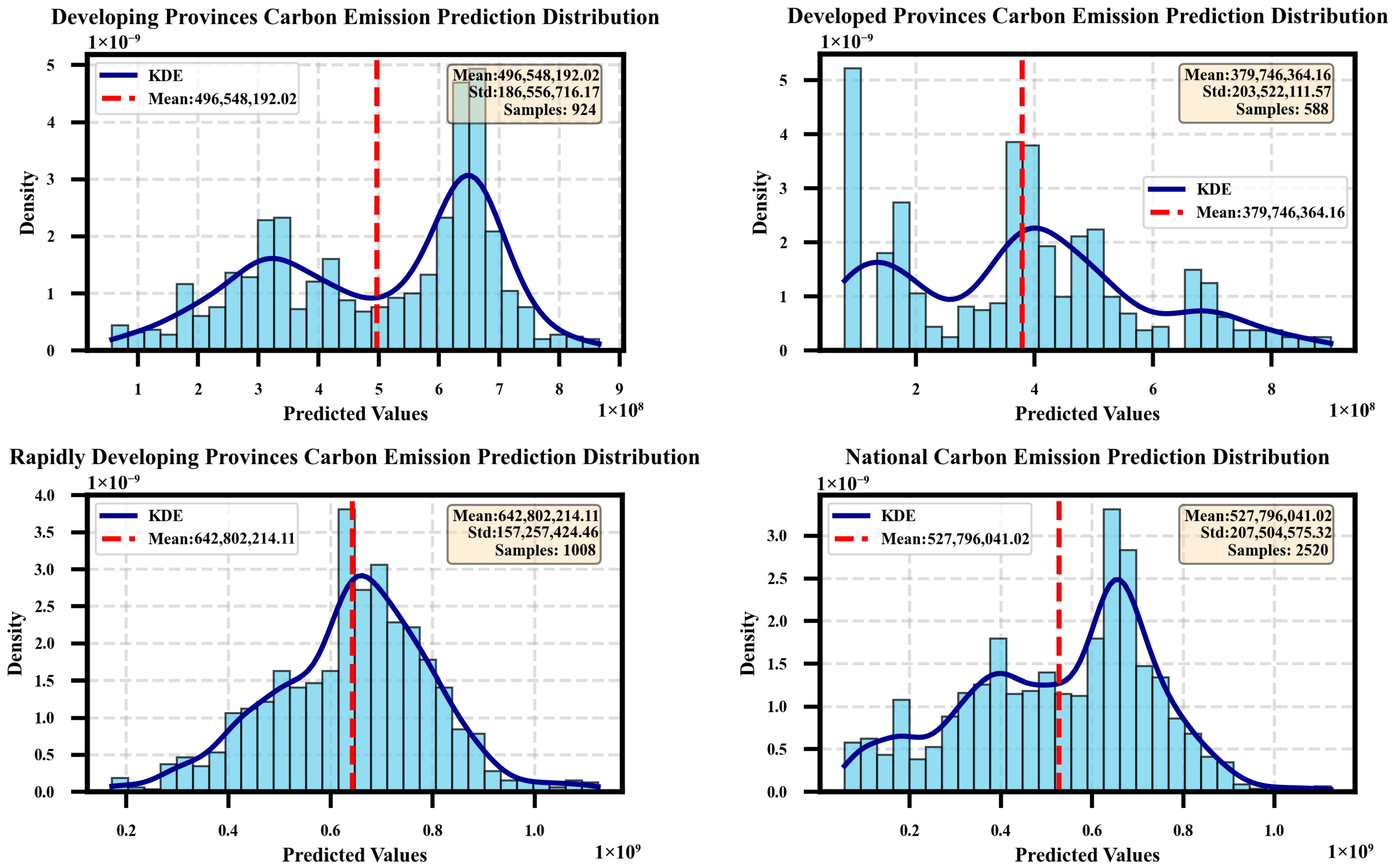
Figure 10 shows the kernel density distribution of forecasted carbon emissions across 30 provincial-level regions (excluding Hong Kong, Macao, and Taiwan). This analysis complements the trajectory-based uncertainty bands in Figure 9 by describing the cross-sectional dispersion and clustering structure of forecast outcomes across provinces, rather than the time-path uncertainty of a single forecast series. The national distribution is right-skewed, with a mean of about 528 million tons and a standard deviation of about 208 million tons. Two relatively clear peaks appear around the 200–400 million ton range and the 600–800 million ton range, indicating two major clusters of provincial emission levels. The right tail extends beyond 1 billion tons, meaning a small number of high-emission provinces lift the national mean noticeably, consistent with strong regional disparities.

By group, developing provinces (including Chongqing, Hainan, Shanxi, and Inner Mongolia among 12 provinces) display a pronounced bimodal pattern. The main peak is around 640 million tons and the secondary peak around 360 million tons, with a clear dip between them. This points to internal divergence: some provinces are in a faster industrialization phase with rapidly rising emissions, while others remain at lower levels due to constraints in resource endowments and industrial structure. The shape also suggests a sensitive transition period in their emissions trajectory. Rapidly developing provinces (including Shandong, Hebei, Liaoning, and Hubei among 13 provinces) show a unimodal, right-skewed distribution with a peak near 700 million tons. Most observations fall in the 500–800 million ton range, and dispersion is relatively low (standard deviation about 157 million tons; coefficient of variation about 0.244), indicating more similarity within the group. The right tail reflects a few provinces that sit slightly above the group mean, but overall differences remain limited.

From an uncertainty perspective, the kernel density results indicate that forecast uncertainty in this study is not only temporal (as reflected by widening uncertainty bands) but also distributional across provinces. In particular, the bimodal pattern in developing provinces suggests heterogeneous transition pathways within the same broad development group, which increases the uncertainty of group-level policy implementation if uniform assumptions are applied. At the same time, these distributional results do not eliminate the possibility of structural breaks in future trajectories. They should therefore be interpreted jointly with the forecast uncertainty bands and the structural-break discussion in Section 4.2.

5. Recommendation and Conclusions

5.1. Recommendations

The policy implications of this study are derived from the combined evidence of the SSA–LSTM–Transformer forecasts, the SHAP-based driver analysis, and the regional heterogeneity results. The empirical findings indicate that mitigation strategies should be differentiated across both time horizons and development stages, while maintaining a coordinated national transition framework.

The forecast trajectories suggest a clear pattern of regional divergence during 2025–2035, with rapidly developing provinces facing relatively greater mitigation pressure as industrialization and energy demand continue to expand. The projected paths become more convergent by 2050, indicating a gradual narrowing of interprovincial differences in emission levels. This pattern supports a phased policy arrangement. In the near- to medium-term period, national carbon-control targets can be implemented with greater flexibility in provincial pathways, allowing local governments to align mitigation intensity with development stage, resource endowment, and industrial conditions. In the longer term, stronger cross-regional coordination becomes more important, including policy alignment, market integration, and technology diffusion mechanisms that can support convergence under a more unified decarbonization framework.

The SHAP results and heterogeneity analysis indicate that policy priorities should be adjusted according to the dominant driver structure in each province group. At the national level, the energy consumption structure remains the primary positive driver of emissions, while technological innovation shows the strongest mitigating contribution. In developing provinces, the driver pattern is more balanced across multiple factors, which implies that policy design should coordinate energy transition, industrial restructuring, infrastructure upgrading, and livelihood considerations to avoid instability from overly narrow interventions. In rapidly developing provinces, energy structure and industrialization pressure remain prominent, and the possibility of rebound effects should be considered when evaluating technology and efficiency policies under expanding demand. In developed provinces, the stronger mitigation contribution of technological innovation suggests greater policy emphasis on advanced low-carbon technology deployment, system integration, and diffusion channels that can improve adoption in industrializing regions.

The kernel density results provide an additional distributional perspective for policy design. The bimodal pattern in provincial emissions indicates persistent interprovincial differentiation during the transition process, while the narrowing distribution in the later forecast period suggests a gradual movement toward a more balanced low-carbon state. The pronounced internal divergence within developing provinces indicates the need for more granular, province-specific implementation plans rather than uniform targets within the same broad category. Policy coordination should also address the risk of relocating outdated or carbon-intensive capacity to resource-rich regions, since such relocation may delay structural transition and create new sources of long-term carbon lock-in.

5.2. Conclusions

Three main conclusions emerge.

Carbon emission drivers exhibit strong spatiotemporal heterogeneity. At the national level, EES is the primary positive driver, and TIM is the main negative driver. As development levels rise, the mechanism shifts from a “resource- and growth-driven” pattern toward a more technology-led pathway. The geographic detector results further support statistically significant differences in driver strength across developed, rapidly developing, and developing provinces (p < 0.05).

SSA–LSTM–Transformer delivers strong predictive performance. In the ablation tests, the full S + L + T configuration performs best, achieving R² = 0.9911 and NRMSE = 0.0192. In external benchmarks, it outperforms baselines such as BP and XGBoost in both accuracy and error stability. The SSA component also contributes materially to performance gains, indicating that the proposed framework is well suited to large-scale carbon emission forecasting with nonlinear, strongly coupled dynamics.

There is still room to improve. The current inputs do not include external shocks such as extreme weather or sharp energy price swings driven by geopolitical events. Real-time updating is also limited by statistical publication cycles. Future work could incorporate higher-frequency data sources, including satellite-based remote sensing, and introduce macro-level shocks as exogenous variables to improve responsiveness to short-run disruptions and structural breaks.

References

1. Zhao, J.; Kou, L.; Wang, H.; He, X.; Xiong, Z.; Liu, C.; Cui, H. Carbon emission prediction model and analysis in the Yellow River basin based on a machine learning method. Sustainability 2022, 14, 6153. [Google Scholar] [CrossRef] [Scilit]
2. Gu, H.; Wu, L. Pulse fractional grey model application in forecasting global carbon emission. Appl. Energy 2024, 358, 122638. [Google Scholar] [CrossRef] [Scilit]
3. Yang, Y.; Yuan, Y.; Han, Z.; Liu, G. Interpretability analysis for thermal sensation machine learning models: An exploration based on the SHAP approach. Indoor Air 2022, 32, e12984. [Google Scholar] [CrossRef] [Scilit]
4. Xia, X.; Liu, B.; Wang, Q.; Luo, T.; Zhu, W.; Pan, K.; Zhou, Z. Analysis of carbon peak achievement at the provincial level in China: Construction of ensemble prediction models and Monte Carlo simulation. Sustain. Prod. Consum. 2024, 44, 445–461. [Google Scholar] [CrossRef] [Scilit]
5. Feng, X.-D.; Wang, X.-L.; Wen, L.; Yuan, Y.; Zhang, Y.-Q. Research and Prediction Analysis of Key Factors Influencing the Carbon Dioxide Emissions of Countries Along the “Belt and Road” Based on Panel Regression and the AAE Coupling Model. Sustainability 2024, 16, 11014. [Google Scholar] [CrossRef] [Scilit]
6. Feng, D.; Xu, W.; Gao, X.; Yang, Y.; Feng, S.; Yang, X.; Li, H. Carbon emission prediction and the reduction pathway in industrial parks: A scenario analysis based on the integration of the LEAP model with LMDI decomposition. Energies 2023, 16, 7356. [Google Scholar] [CrossRef] [Scilit]
7. Sharma, S.; Mittal, A.; Bansal, M.; Joshi, B.P.; Rayal, A. Forecasting of carbon emissions in India using ARIMA time series predicting approach. In International Conference on Renewable Power; Springer Nature: Singapore, 2023; pp. 799–811. [Google Scholar] [CrossRef] [Scilit]
8. Li, Y.; Chen, Y.; Wang, Y. Grey forecasting the impact of population and GDP on carbon emissions in a Chinese region. J. Clean. Prod. 2023, 425, 139025. [Google Scholar] [CrossRef] [Scilit]
9. Lu, J.; Chen, H.; Cai, X. From global to national scenarios: Exploring carbon emissions to 2050. Energy Strategy Rev. 2022, 41, 100860. [Google Scholar] [CrossRef] [Scilit]
10. Zhao, X.; Du, D. Forecasting carbon dioxide emissions. J. Environ. Manag. 2015, 160, 39–44. [Google Scholar] [CrossRef] [Scilit]
11. Breiman, L. Random forests. Mach. Learn. 2001, 45, 5–32. [Google Scholar] [CrossRef] [Scilit]
12. Cortes, C.; Vapnik, V. Support-vector networks. Mach. Learn. 1995, 20, 273–297. [Google Scholar] [CrossRef] [Scilit]
13. Chen, T.; Guestrin, C. XGBoost: A scalable tree boosting system. In Proceedings of the 22nd ACM SIGKDD International Conference on Knowledge Discovery and Data Mining, San Francisco, CA, USA, 13–17 August 2016; pp. 785–794. [Google Scholar] [CrossRef] [Scilit]
14. Wang, H.; Wei, Z.; Fang, T.; Xie, Q.; Li, R.; Fang, D. Carbon emissions prediction based on the GIOWA combination forecasting model: A case study of China. J. Clean. Prod. 2024, 445, 141340. [Google Scholar] [CrossRef] [Scilit]
15. Bhatt, H.; Davawala, M.; Joshi, T.; Shah, M.; Unnarkat, A. Forecasting and mitigation of global environmental carbon dioxide emission using machine learning techniques. Clean. Chem. Eng. 2023, 5, 100095. [Google Scholar] [CrossRef] [Scilit]
16. Han, Z.; Cui, B.; Xu, L.; Wang, J.; Guo, Z. Coupling LSTM and CNN neural networks for accurate carbon emission prediction in 30 Chinese provinces. Sustainability 2023, 15, 13934. [Google Scholar] [CrossRef] [Scilit]
17. Wang, T.; Fu, Z.; Zhang, S.; Li, Z. Water erosion risk assessment and predictive modelling for cultural heritage under climate change: A case study of the Great Wall in the Yellow River Basin, China. J. Clean. Prod. 2025, 510, 145645. [Google Scholar] [CrossRef] [Scilit]
18. Fu, Z.; Yang, X.; Ma, Y.; Sun, Y.; Wang, T. Integrating explainable AI and causal inference to unveil regional air quality drivers in China. J. Environ. Manag. 2025, 390, 126270. [Google Scholar] [CrossRef] [Scilit] [PubMed]
19. Sun, Q.; Chen, H.; Long, R.; Zhang, J.; Yang, M.; Huang, H.; Ma, W.; Wang, Y. Can Chinese cities reach their carbon peaks on time? Scenario analysis based on machine learning and LMDI decomposition. Appl. Energy 2023, 340, 121427. [Google Scholar] [CrossRef] [Scilit]
20. Zhao, X.; Long, L.; Yin, S.; Zhou, Y. How technological innovation influences carbon emission efficiency for sustainable development? Evidence from China. Resour. Environ. Sustain. 2023, 14, 100135. [Google Scholar] [CrossRef] [Scilit]
21. Wang, Z.; Shao, H. Spatiotemporal interactions and influencing factors for carbon emission efficiency of cities in the Yangtze River Economic Belt, China. Sustain. Cities Soc. 2024, 103, 105248. [Google Scholar] [CrossRef] [Scilit]
22. Ma, D.; Deng, P.; Yan, Y.; Zhang, J.; Guo, Z.; Hu, C.; Li, K. How does carbon emission efficiency vary in Chinese cities? Taking 108 cities along the Yangtze River Economic Belt as an example. Renew. Energy 2026, 256, 124208. [Google Scholar] [CrossRef] [Scilit]
23. Xu, P.; Zhou, G.; Zhao, Q.; Lu, Y.; Chen, J. Spatiotemporal dynamics and influencing factors of city-level carbon emissions in mainland China. Ecol. Indic. 2024, 167, 112672. [Google Scholar] [CrossRef] [Scilit]
24. Pan, X.; Guo, S. Decomposition analysis of regional differences in China’s carbon emissions based on socioeconomic factors. Energy 2024, 303, 131932. [Google Scholar] [CrossRef] [Scilit]
25. Zhou, Y.; Song, M.; Xu, W.; Ouyang, W. Empowering carbon neutrality: Impact of the technology factor market on China’s carbon emission intensity. J. Environ. Manag. 2025, 391, 126568. [Google Scholar] [CrossRef] [Scilit]
26. Cheng, H.; Wu, B.; Jiang, X. Spatial network structure of energy carbon emission efficiency and its driving factors in Chinese cities. Appl. Energy 2024, 371, 123689. [Google Scholar] [CrossRef] [Scilit]
27. Xin, L.; Li, S.; Rene, E.R.; Lun, X.; Zhang, P.; Ma, W. Prediction of carbon emissions peak and carbon neutrality based on life cycle CO2 emissions in megacity building sector: Dynamic scenario simulations of Beijing. Environ. Res. 2023, 238, 117160. [Google Scholar] [CrossRef] [Scilit]
28. Huo, T.; Xu, L.; Feng, W.; Cai, W.; Liu, B. Dynamic scenario simulations of carbon emission peak in China’s city-scale urban residential building sector through 2050. Energy Policy 2021, 159, 112612. [Google Scholar] [CrossRef] [Scilit]
29. Li, W.; Wen, H.; Nie, P. Prediction of China’s industrial carbon peak: Based on GDIM-MC model and LSTM-NN model. Energy Strategy Rev. 2023, 50, 101240. [Google Scholar] [CrossRef] [Scilit]
30. Alabi, R.O.; Elmusrati, M.; Leivo, I.; Almangush, A.; Mäkitie, A.A. Machine learning explainability in nasopharyngeal cancer survival using LIME and SHAP. Sci. Rep. 2023, 13, 8984. [Google Scholar] [CrossRef] [Scilit]
31. Hochreiter, S.; Schmidhuber, J. Long short-term memory. Neural Comput. 1997, 9, 1735–1780. [Google Scholar] [CrossRef] [Scilit] [PubMed]
32. Guo, Y.; Mao, Z. Long-term prediction model for NOx emission based on LSTM–Transformer. Electronics 2023, 12, 3929. [Google Scholar] [CrossRef] [Scilit]
33. Si, Q.; Li, Y.; Sun, J.; Yu, X.; Li, J.; Wang, J.; Dong, X.; Guo, K. New energy vehicle forecasting based on grey forecasting and random forest. In Smart Applications and Sustainability in the AIoT Era; Al-Turjman, F., Ed.; Springer: Cham, Switzerland, 2024. [Google Scholar] [CrossRef] [Scilit]
34. Qiu, C.; Li, Q.; Jing, J.; Tan, N.; Wu, J.; Wang, M.; Li, Q. Transforming prediction into decision: Leveraging Transformer-long short-term memory networks and automatic control for enhanced water treatment efficiency and sustainability. Sensors 2025, 25, 1652. [Google Scholar] [CrossRef] [Scilit] [PubMed]
35. Li, Y.; Wang, Z.; Yang, A.; Yu, X. Integrating evolutionary algorithms and enhanced-YOLOv8+ for comprehensive apple ripeness prediction. Sci. Rep. 2025, 15, 7307. [Google Scholar] [CrossRef] [Scilit]
36. Chen, X.; Liu, X.; Luo, Y.; Zeng, X. Exploring time-series deep learning models for ship fuel consumption prediction. J. Mar. Sci. Eng. 2025, 13, 2102. [Google Scholar] [CrossRef] [Scilit]
37. Li, Y.; Song, Z.; Xia, L.; Sun, J.; Wang, Z. Application of the adaptive sparrow search algorithm in medical supply engineering. Sci. Rep. 2025, 15, 35775. [Google Scholar] [CrossRef] [Scilit]
38. Lee, K.; Ko, J.; Jung, S. Quantifying uncertainty in carbon emission estimation: Metrics and methodologies. J. Clean. Prod. 2024, 451, 142141. [Google Scholar] [CrossRef] [Scilit]
39. Akrami, M.; Porter, M.D.; Colosi, L.M. Addressing uncertainty in machine learning-integrated life cycle assessment. J. Environ. Manag. 2025, 375, 126225. [Google Scholar] [CrossRef] [Scilit]
40. Xu, H.; Pan, X.; Guo, S.; Lu, Y. Forecasting Chinese CO2 emissions using a nonlinear multi-agent intertemporal optimization model and scenario analysis. Energy 2021, 229, 120514. [Google Scholar] [CrossRef] [Scilit]
41. Yu, W.; Xia, L.; Cao, Q.; Ni, J. A machine learning algorithm to explore the drivers of carbon emissions in Chinese cities. Sci. Rep. 2024, 14, 13490. [Google Scholar] [CrossRef] [Scilit]
42. Ke, Z.; Cao, Y.; Chen, Z.; Yin, Y.; He, S.; Cheng, Y. Early warning of cryptocurrency reversal risks via multi-source data. Financ. Res. Lett. 2025, 85, 107890. [Google Scholar] [CrossRef] [Scilit]
43. Zong, K.; Shen, J.; Zhao, X.; Fu, X.; Wang, Y.; Li, Z.; Liu, L.; Mu, H. A stable technical feature with GRU-CNN-GA fusion. Appl. Soft Comput. 2026, 187, 114302. [Google Scholar] [CrossRef] [Scilit]
Figure 1. Research framework diagram.
Sustainability 18 02893 g001
Figure 2. Diagram of LSTM–SHAP.
Sustainability 18 02893 g002
Figure 3. LSTM–Transformer model framework.
Sustainability 18 02893 g003
Figure 4. SSA workflow.
Sustainability 18 02893 g004
Figure 5. SHAP results for carbon emission drivers.
Sustainability 18 02893 g005
Figure 6. Regional heterogeneity in SHAP-based driver effects.
Sustainability 18 02893 g006
Figure 7. Tests of regional heterogeneity for carbon emission drivers.
Sustainability 18 02893 g007
Figure 8. Iterative results of SSA search and other search methods.
Sustainability 18 02893 g008
Figure 9. Mean forecasts of carbon emissions for provinces and the national total.
Sustainability 18 02893 g009
Figure 10. Kernel density distribution of forecasted emissions.
Sustainability 18 02893 g010