A Two-Stage Model for Optimizing Intercity Multimodal Timetables and Passenger Flow Assignment Under Multiple Uncertainty Within Urban Agglomerations

Abstract

In order to maximize passenger travel satisfaction and enhance the sustainability of the intercity multimodal transportation system, this paper proposes a two-stage model for intercity multimodal timetable coordination optimization under uncertainty. In the first stage, a robust spatio-temporal graph is built to allocate intermodal passenger flows in order to determine passengers’ route selection results to minimize the total travel cost. At the same time, explicit capacity constraints and transfer behaviors are considered in order to be more realistic. In addition, passengers can take multiple transportation modes (High-speed Rail, Ordinary Rail, EMU, and Coach) in a single trip. The outputs of the first stage are subsequently integrated into the second-stage interval multi-objective timetable optimization model to determine departure times and stopping patterns under uncertain dwell and travel times. It is able to achieve the maximum reduction of passenger travelling time and waiting time within the minimum timetable adjustment, which further improves the integration level of transportation services. To ensure the diversity and convergence of model solving on the basis of retaining uncertain information, we propose an integrated algorithm PSO-IMOEA-MC involving Particle Swarm Optimization algorithm (PSO) and Interval Many-objective Evolutionary Algorithm combined with Monte Carlo (IMOEA-MC). Finally, the effectiveness of the proposed two-stage model and algorithm is validated using three intercity networks: Beijing–Zhangjiakou, Chengdu–Chongqing, and Guangzhou–Qingyuan. The results demonstrate the performance of the method in finding high-level solutions that retain more uncertainty. The findings of this study provide technical support for timetable adjustments under diverse operational scenarios.

1. Introduction

China urgently needs to promote the construction of a comprehensive national transport network to achieve coordinated development of multiple transportation modes and a high-level dynamic balance between demand and supply. This is critical for constructing a green and low-carbon urban agglomeration transportation system [1,2], reducing the overall energy consumption and emissions of the transportation system, and achieving sustainable development. Furthermore, some methods and solutions in traffic and transportation engineering have also been proposed to support energy saving in smart cities and guide the future development of transportation networks [3]. The intercity multimodal transportation system consists of several modes, routes, and vehicles at stations [4]. However, due to the lack of synergy between various modes of transport and the problem of non-synchronous schedules, when passengers freely choose travel time, travel mode and vehicle, the distribution of passenger flow in the system is often uneven. Long waiting time and long transfer time reduce passengers’ travel efficiency and satisfaction. Timetable optimization is closely related to passenger flow assignment. The initial timetable cannot well meet the dynamic and changing passenger flow. Therefore, it is necessary to design an appropriate quantitative evaluation framework for synchronization objectives to reflect the sensitivity of passengers to timetable optimization. In addition, decision makers should also be taken into account, especially their acceptance of timetable adjustment deviations.

For intercity passenger routing, flow assignment models are a well-studied issue that can predict passenger behavior [5] These models take passenger perceived cost as input and are represented by time-in-vehicle, comfort, expenses, etc. However, passengers’ perceived cost varies with timetable adjustment, and passenger routing also changes. Dynamic optimization makes the problem more complex.

At the same time, uncertainty runs through the entire process. Delay, parking time, and other uncertainties affect the generation and decision-making of optimization schemes. There have been many studies on calibrating uncertain parameters [6]. However, as far as we know, the most advanced methods cannot take all uncertainties into account. Considering only one or part of the uncertainty leads to unsatisfactory results. Therefore, it is necessary to comprehensively describe the multiple uncertainties, so that the solution set obtained contains all possibilities and ensures the robustness of the optimized timetable.

Some studies have used an iterative approach to simultaneously optimize schedules and assign passenger flows [7], but this approach is not conducive to the diversity of solution sets. In some complex problems, it may even result in failure to find a feasible solution. In order to overcome the problems of previous research, this paper proposes a collaborative optimization method for solving uncertainty in the timetable and passenger flow under the condition that passengers can freely choose combinations of multiple transport modes and train capacity constraints. Meanwhile, we constructed a two-stage hybrid planning model.

In the first stage, we allocate multimodal passenger flow with the goal of minimizing passenger travel costs. We propose an optimized multimodal route selection model, which determines the passenger flow of each route and each vehicle. We use particle swarm optimization (PSO) to solve the problem.

In the second stage, we optimize the multimodal timetable, introducing interval mathematics, minimizing passenger travel time, waiting time, and adjustment time, determining a timetable optimization scheme that includes departure time, parking time, and skip-stopping. We use an interval many-objective evolutionary algorithm based on Monte Carlo simulation to solve this problem.

We apply our model and algorithm on three intercity networks including Beijing–Zhangjiakou, Chengdu–Chongqing, and Guangzhou–Qingyuan. The results show that our proposed method can find solutions with better diversity and convergence in an efficient manner under any uncertain conditions.

The main contributions of this paper are summarized as follows, which are predicated on the multiple assumptions detailed in Section 3 (specifically regarding passenger familiarity with timetables, First-In-First-Out (FIFO) boarding rules, and operational uncertainty):

(1)

Aiming at the low matching degree between path-level travel demand and multimodal transport supply, a two-stage model for intercity multimodal passenger flow assignment and timetable optimization under uncertain parameters is developed. The model optimizes departure time and parking patterns under dynamic decision environments and effectively shrinks the search space of the solution set while coordinating passenger routing and timetable adjustment.

(2)

To fully reflect the impact of uncertainties and simultaneously ensure the diversity and convergence of solutions, an integrated algorithm PSO-IMOEA-MC combining particle swarm optimization, interval many-objective evolutionary algorithm, and Monte Carlo simulation is proposed to solve the two-stage model.

(3)

The proposed model is tested on three intercity networks in different urban agglomerations. The results show that the algorithm can capture the influence of uncertain parameters in the solution set and obtain a set of optimal timetable schemes, demonstrating the effectiveness and advantages of the proposed two-stage model and solution approach.

The rest of this article is as follows. Section 2 reviews the relevant contributions of timetable optimization and passenger flow assignment. Section 3 describes the problem to be solved. Section 4 provides an overview structure of the two-stage model. The details of this model’s two sub models will be described in Section 5 and Section 6. Section 7 is an example verification. Finally, Section 8 summarizes the entire paper and proposes future research directions.

2. Literature Review

2.1. Collaborative Optimization Model for Multimodal Timetables

A problem involving three or more objectives is generally referred to as a many-objective optimization problem (MOP). Timetable optimization falls into this category, as it considers both passenger convenience and operator efficiency. Existing studies mainly focus on a single objective and aim to obtain a deterministic optimal solution [8,9,10]. However, when passengers are free to choose their travel options, existing studies become insufficient. Therefore, we propose a many-objective hybrid planning model to optimize intercity multimodal timetables considering time window constraints, capacity constraints, and transfer constraints, etc.

In practice, some parameters in the objective function and constraints often contain uncertainty. These values are imprecise, representing the uncertainty of the model and the instability of the system, such as train delays caused by extreme weather, long dwell times caused by passenger flow, etc. [11].

Many parameters in practical problems can be represented by intervals. For example, the length of a spring can be represented by the length in two states of being compressed and stretched as the extreme values of the interval. Uncertainty can naturally be modeled using interval representations. Considering interval parameters on the basis of general many-objective optimization problems are called interval many-objective optimization problems (IMOPs) [12,13]. Compared with deterministic many-objective optimization, research on IMOPs remains relatively limited.

Some studies have addressed uncertainty through random variables and robust optimization, but they cannot fully reflect the uncertainty problem. For example, the random variable method relies on accurate probability distribution information, which is difficult to obtain [14]. Robust optimization tends to be conservative and may overlook potentially superior solutions [15], making it less suitable for the timetable optimization problem considered in this study. Interval multi-objective optimization is a more flexible method that can consider the entire possible range of the problem and can more fully reflect the nature of the problem. Its application prospects in practical problems are also very broad.

Many-objective evolutionary algorithms (MOEAs) can be divided into three types [16]. Among them, Pareto dominance-based methods have good convergence and poor diversity [17], while indicator-based algorithms exhibit superior diversity maintenance, but their effectiveness critically depends on the availability of precise objective values [18]. However, previous MOEAs cannot directly handle IMOPs because their objective function values are intervals.

Existing approaches for solving IMOPs can be broadly categorized into two types. The first method transforms interval objectives into deterministic formulations or relaxes them through approximate treatments [19]. There are also many studies that use the robust optimization method described earlier to relax the objective function [20,21], but how to set it is also a scientific problem. As mentioned earlier, this method cannot fully consider the problem, and the solution set is difficult to fully reflect uncertain parameters.

The second approach develops an IMOEA based on interval partial order relations and performance indicators [22,23], thereby generating an interval Pareto front. However, for practical application problems such as timetable optimization, there is no absolute best or worst model, and better solutions may be found under different parameter combinations. Therefore, we integrate the Monte Carlo algorithm and propose an IMOEA combined with Monte Carlo (IMOEA-MC) for scene optimization.

Determining the exact global optimal solution of Time Table Problem (TTP) is an NP-hard problem [24]. The uncertainty places higher demands on algorithm’s diversity and efficiency. As an early algorithm, Non-dominated Sorting Genetic Algorithm II (NSGA-II) has not been completely updated. Conversely, it has continued to show its potential in terms of convergence and efficiency. Therefore, this study expanded search space caused by mutual iteration by using a two-stage structure and applied the Monte Carlo algorithm to sample multiple intervals to ensure diversity of solutions. Meanwhile, an interval many-objective evolutionary algorithm based on NSGA-II is constructed to improve the convergence and efficiency.

2.2. Passenger Flow Assignment in Timetable Optimization

Due to limited capacity and the fact that passengers tend to select routes with the lowest generalized cost, not all passengers are able to travel according to their desired route. Therefore, we should consider capacity, and reasonably arrange passengers on route as much as possible. Some researchers have imposed limitations on the passenger flow for each train [25], while others have allocated passengers based on the FIFO principle [26], and still others have required that the number of incoming passengers must be less than the train’s capacity [27]. However, these constraints do not fully align with the real-world scenarios of passenger ticket purchasing and queuing. However, in such a system, there may be a large number of passengers unable to board the train, which is not practical and not conducive to retaining passengers. To relax these assumptions, some scholars have adopted the Logit model [28] to calculate the possibility of passengers switching to another transportation mode, but this requires travel information of other transportation modes. In order to solve the data problem, a study divides passengers into several groups and assigns each group to a path [29]; if there is no path due to train capacity limitations, it is assumed that the passenger group is traveling outside the planned range. But in fact, some passengers within the same passenger group can travel within the planned range. Therefore, the allocation method should be modified. For demand exceeding capacity, we plan a virtual path with no capacity limitations and impose sufficient costs on the virtual path in a punitive manner to maintain the complete operation of the system.

Representing activity schedule decisions as path selection in spatiotemporal networks is an emerging method. As mentioned earlier, the Logit model is a typical form of path selection model. For example, Lu T et al. [30] used the Multinomial Logit (MNL) [31] model to calculate the selection results of passengers for different modes, but he did not consider transfers or routes composed of multiple modes. Hartleb J used a Logit model to approximate passenger distribution [32] and integrated passenger distribution into the timetable optimization framework, achieving quantification of the impact of multiple paths on timetable optimization, but it also does not consider multiple modes and passengers’ transfer. We design a path selection model and define a generalized cost function considering transfer. Prior to this, a multimodal spatiotemporal network between cities was designed to assign temporal and spatial attributes to vehicles, stations, etc., achieving dynamic changes in paths and dynamic path selection of passenger flow.

However, the variance of the utility function in the Logit model is fixed, which does not align with the actual situation. The Weibit models can solve the heterogeneity problem in the Logit model [33]. In our previous research, we compared the Logit and Weibit models and proposed a Two-Stage Path-Size Weibit (TS-PSW) model that is more suitable for long distance travel [34]. This paper optimizes the proposed model again and optimizes the uncertainty parameters in the model to make passenger flow allocation closer to the actual situation.

Overall, timetable optimization has been widely recognized as an effective approach to balancing operational supply and passenger demand and improving travel efficiency. However, most existing studies focus on single transport modes or consider multimodal systems under the assumption of fixed passenger demand. Research explicitly addressing intercity multimodal timetable optimization with elastic passenger choice remains limited. Furthermore, timetable optimization and passenger flow assignment are often investigated separately. Only a small number of studies attempt to jointly model timetable-based passenger allocation and passenger-response-based timetable adjustment, and these are generally confined to single-mode operational systems rather than integrated multimodal networks. As a result, the coordinated optimization of passenger flows and timetables in intercity multimodal systems is still insufficiently explored. To address these gaps, this study proposes a two-stage framework integrating a multimodal passenger flow assignment model with an interval many-objective timetable optimization model. By structurally coupling passenger allocation and timetable adjustment, the framework expands the effective search space at the modeling level and reduces the risk of local optima or infeasible solutions, thereby generating a set of optimized and implementable timetable schemes.

3. Problem Description

The collaborative optimization problem of multimodal timetable and passenger flow under multiple sources of uncertainty can be described as follows. In the first stage, we set all hub stations of origin and destination stations, and the user’s departure station, destination station, and departure time. Then, we find the most ideal path for all passengers based on the original timetable. If a path contains multiple selected trains, if passengers transfer, they can get off at the transfer station and then get on the next selected train. Otherwise, a train will go directly from the departure point to the destination.

Therefore, we can obtain the optimal passenger flow assignment under the original timetable. By inputting the passenger flow allocation results as known conditions into the second stage (multimodal timetable optimization model), we can find the timetable optimization scheme with the minimum adjustment amplitude and maximum optimization effect. The optimization scheme includes: (1) departure time at the origin station, (2) arrival and departure time at the transfer station, (3) dwell time at the stopping station, and (4) the dwell status at the stopping station. The timetable optimization considers dwell status constraint, time window constraints, transfer constraint, overtaking constraint, etc., which simulates the actual operation situation more realistically.

In order to facilitate our comprehensive modeling of the timetable, passenger allocation, and vehicle scheduling involved in this problem, several assumptions will be made as follows:

Assumption 1.

Assuming that all passengers are frequent users familiar with the timetables and will adjust their departure and arrival time based on the timetable.

Assumption 2.

Assuming that vehicles do not operate accurately according to the timetable.

Assumption 3.

Assuming there are two tracks in the same direction of the station, one for trains arriving and stopping. The other serves non-stop trains for passing by.

Assumption 4.

Assuming that the passenger flow is allocated according to the passenger assignment model proposed in Section 5.

Assumption 5.

Assuming that passenger path selection and passenger flow allocation do not consider the process before passengers arriving at the station.

Assumption 6.

Assuming that all passengers board on FIFO basis. When passengers are unable to board a fully loaded train, they wait for the next train.

At the same time, we have considered some limitations on the feasible path set in terms of passenger flow allocation to enhance the likelihood of swiftly identifying viable solutions at the granular level. We study the proposed method for solving optimization problems under uncertain conditions based on the interaction between multiple modes of transportation timetables, capacity, and path selection.

In the first stage, we set the objective as minimizing the total cost of the system. In the second stage, we quantify these interactions through four objectives: (1) minimizing the total travel time, (2) minimizing the total wait time, (3) minimizing the total adjustment time, and (4) minimizing the total parking mode changes. These four goals also reflect the preferences of the main participants in intercity transportation services, that is, vehicle operating companies, passengers, and infrastructure managers.

4. Algorithmic Overview

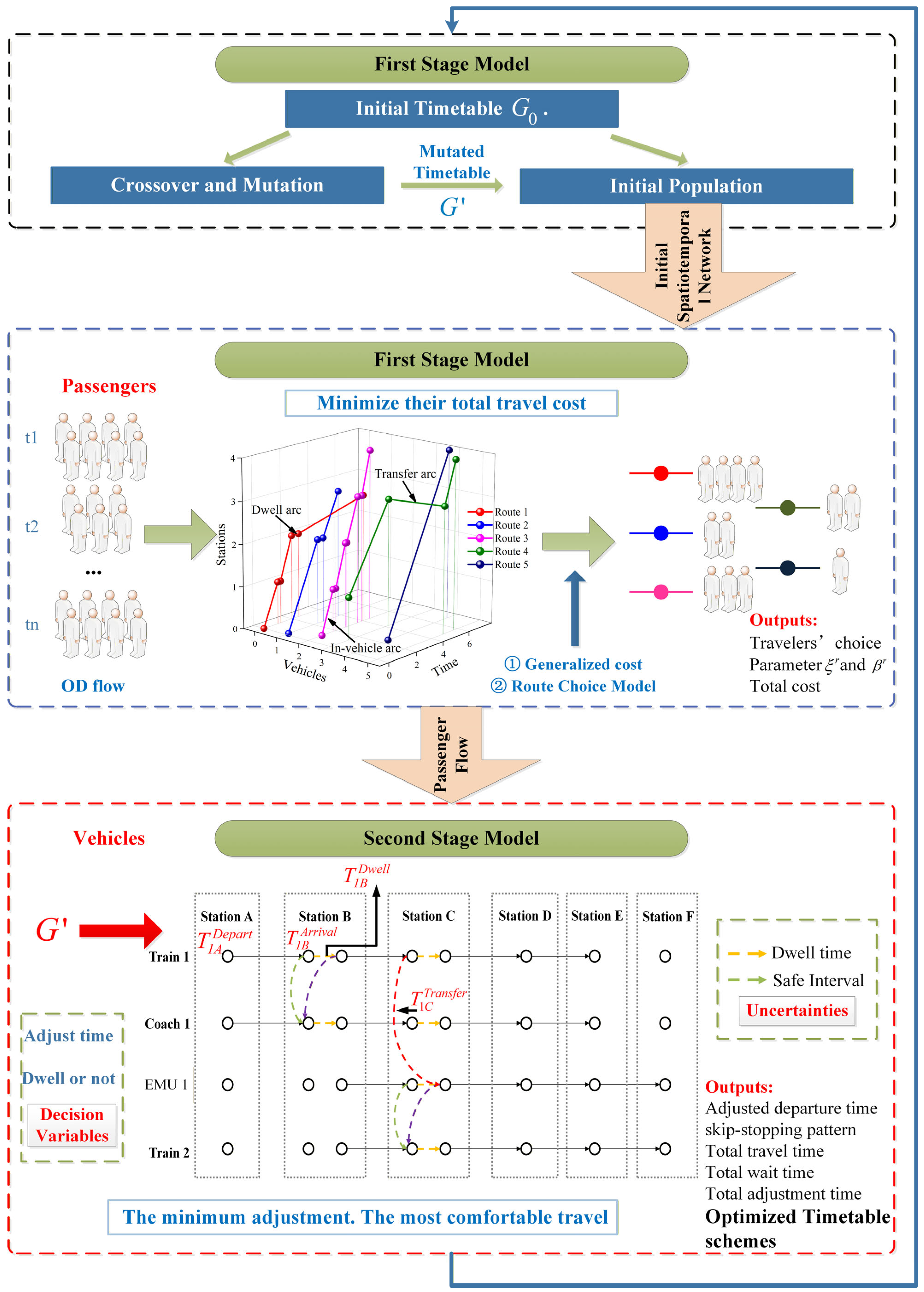
As shown in Section 3, this paper studies many-objective two-stage mixed programming problems, which involve multiple uncertainties such as travel time, dwell time, etc. The overall structure of the two-stage model is shown in Figure 1.

In order to ensure a feasible timetable under any uncertainty, we propose an algorithm framework that mainly integrates Monte Carlo and IMOEA based on NSGA-II with PSO to solve. The algorithm takes the original timetable and OD passenger demand as inputs. The problem is solved sequentially according to the two-stage model structure. Passenger flow is input into the passenger flow allocation model, with the goal of minimizing system cost, and we use PSO to optimize the passenger flow (Section 5). Then, passenger flow is input into the timetable optimization model, and the concept of interval mathematics is introduced. Meanwhile, we consider constraints such as capacity and time window and use the IMOEA-MC algorithm to obtain a new feasible timetable scheme (Section 6).

Upon obtaining the initial passenger flow assignment and the corresponding timetable optimization scheme based on the above process, the optimized timetable is fed back as input to the initialization stage. This triggers an update of the time–space graph, followed by a re-assignment of passenger flow and a subsequent round of timetable optimization. This iterative cycle continues until an optimal and convergent timetable solution is achieved.

5. Passenger Assignment

5.1. Passenger Decision

In order to describe the problem more appropriately, it is necessary to first construct an intercity transportation network and introduce the calculation of passengers’ multimodal travel costs. On this basis, we propose the two-stage model.

5.1.1. Passenger and Network Definition

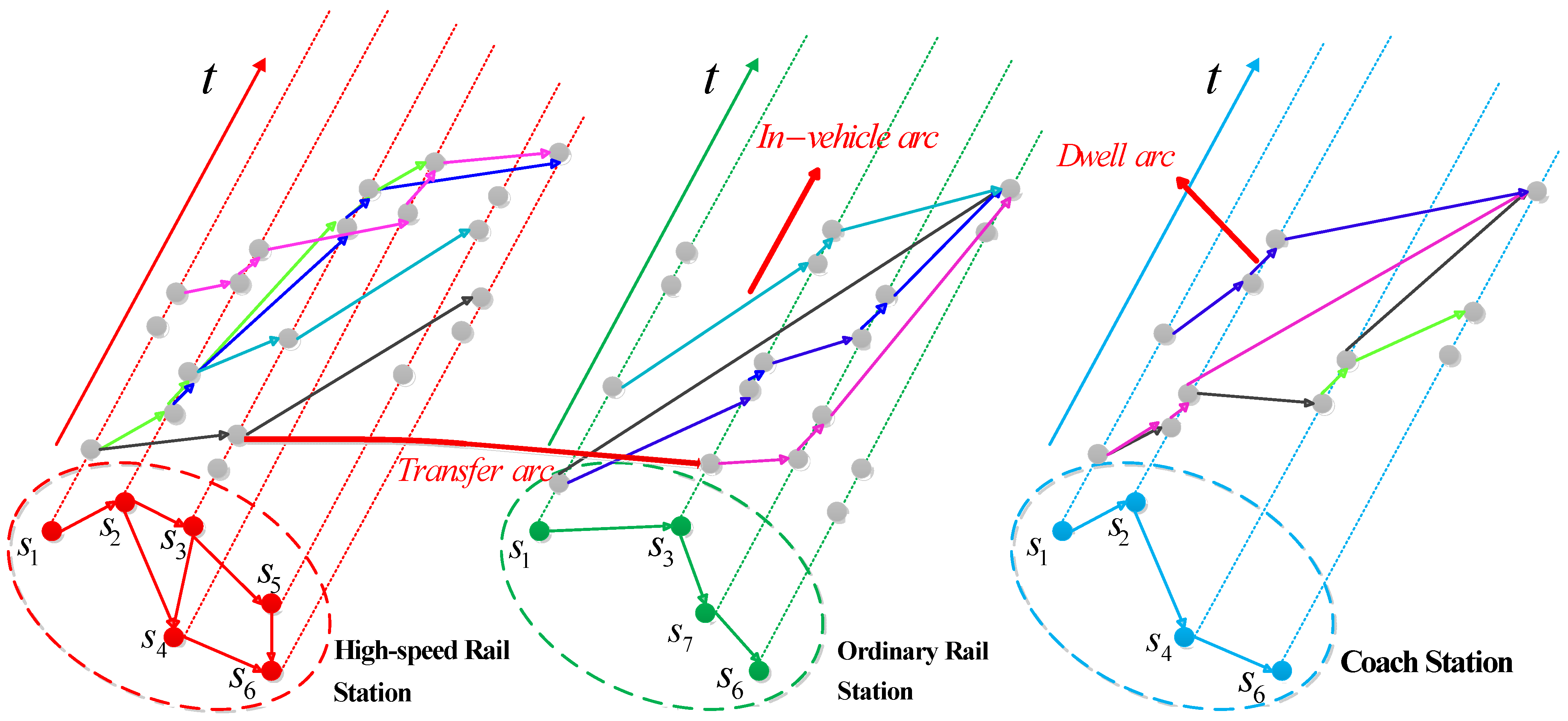
We define the intercity transportation network as $G=(V,E)$ and use a spatiotemporal network representation for passenger assignment, which is shown as Figure 2. Where the node set is denoted as $V=(v_1,v_2,\dots ,v_m)$, $m=S\times H\times N$. Stations that train $n$ passes through are $S_n\subseteq S$, stations that train $n$ must pass through are $\overline{S_n}\subseteq S_n$, train set is $N=\{1,2,\dots ,n\}$. $H=(0,\tau ,2\tau ,\mathrm{\dots },\upsilon \tau )$ involves $\upsilon +1$ time intervals, and each node can be represented as $v_i=(s,t,n)$, which means station, time, and train number. $E$ is the arc set of $G$, and the arcs connecting $v_i,v_j$ are represented by $[v_i,v_j]$, $E=E_{IVT}\cup E_{WAIT}\cup E_{TRF}\cup E_{WALK}\cup E_{PUN}$, representing the set of in-vehicle arcs, waiting arcs, transfer arcs, walk arcs, and penalty arcs. The set of spatiotemporal arcs that train $n$ can occupy is $E_i\subset E$. $(s,t,n)\in V$ is the spatiotemporal network node index, and $(s,t,n\to s^{\prime },t^{\prime },n^{\prime })\in E$ is the arc index. Among them, the in-vehicle arc cost consists of three factors: travel time cost $T_p^{IVT}$, comfort cost $T_p^{COMFORT}$, and expense $E_p^{EXPENSE}$. Let $j\in J$ be a group of passengers entering the station at $t$. Each passenger can be represented by $(O_j,D_j,t_j)$, $O_j,D_j\in S$, $t_j\in H$, $t_j$ represents the arrival time of passenger $j$. A group enters at the same time.

The multimodal transportation spatiotemporal network requires real-time data sharing and integration, including information such as multimodal timetables and passenger demand. However, difficulties and obstacles still exist in data sharing and integration between different transportation modes and related departments. Therefore, this study employs a graph-theoretic approach to construct an intercity multimodal transportation network within the urban agglomeration, considering the interrelationships and connection methods between various transportation modes. The required inputs mainly include published timetables, vehicle capacities, and hub transfer relationships.

As this study focuses on intercity travel, long-distance out-of-station transfers are generally not considered. Cross-modal transfers (e.g., Rail-to-Coach) are modeled only within integrated hub stations. In the spatiotemporal network, same-station transfers and cross-modal transfers share similar topological representations, but their transfer costs are calculated separately to reflect differences in convenience, coordination, and walking time.

The spatiotemporal network (Figure 2) is dynamically changing. On the one hand, arcs’ weight will change with the loading of passengers, thus affecting the path selection of the next passenger group. On the other hand, the nodes will change with timetable adjustment, which may increase or decrease nodes, leading to changes in the path. We use Depth-First-Search algorithm (DFS) to search for feasible paths.

5.1.2. Path Generalized Cost Function

The variables and parameters involved in this chapter are shown in

Table 1. Parameters.

Notations	Description
$r$	OD pair
$p$	Path
$\tilde{p}$	Virtual path
$n,n\prime$	Train
$s,s\prime$	Station
$S_p$	Stations on path $p$
$P_r$	Set of all paths $p$ on $r$
$n_p^{origin}$	Origin station of train $n$ on $p$
$n_p^{transfer}$	Transfer station of train $n$ on $p$
$t_{ns\prime }^{Arrival}$	Arrival time of train $n$ at station $s$
$t_{ns}^{Depart}$	Departure time of train $n$ at station $s$
$d_{nss\prime }^{crowd}$	Crowding coefficient of train $n$ between intervals $[s,s\prime ]$
$x_{ss\prime }$	Passenger flow of train $n$ between intervals $[s,s\prime ]$
$S_{ss\prime }$	Seating capacity of train $n$ between intervals $[s,s\prime ]$
$C_{ss\prime }$	Capacity of train $n$ between intervals $[s,s\prime ]$
$t_{nss\prime }^{COMFORT}$	Comfort of train $n$ between intervals $[s,s\prime ]$
$T_{ns}^{Wait}$	The maximum waiting time interval for passengers at station $s$ (min)
$t_n^{wait}$	Waiting time interval for train $n$ (min)
$i_n^{wait}$	Number of $T_{ns}^{Wait}$ in the origin zone for path $p$
$t_{nn\prime }^{Walk}$	Walking time that passengers spend on transfer from train $n$ to train $n\prime$ (min)
$e_{nss\prime }$	Expenses of train $n$ between intervals $[s,s\prime ]$ (yuan)
$t_{s^{trf}}^{nn\prime }$	Transfer time interval from train $n$ to train $n\prime$ at station $s^{trf}$ (min)
$N_{s^{trf}}$	Transfer times
$C_p^r$	Generalized cost of path p on r, which is calculated by $f_k(q_k)$
${\omega }_p^r$	Path size factor
$l_p$	Length of path $p$ (m)
$L_P^r$	The total length of all paths $p$ on $r$ (m)
$I$	Per capita annual income of residents (yuan)
$W$	Legal working hours (hours)
$D$	Legal working days (days)
$H$	Ultimate time to recover fatigue (hours), $H=15 h$
$\overline{t}$	Average travel time (min)
$\epsilon \overline{t}$	Acceptable delay time (min)
$\delta ,{\xi }^r,{\beta }^r$	Pending parameters
$L_{nn\prime }$	Walking length from train $n$ to train $n\prime$ (m)
$V$	Walking speed (m/s)

.

We have previously studied which factors have an impact on passenger choices [34]. Therefore, we continue to establish generalized cost function based on these influencing factors.

(1)

$E_{IVT}:(s,t,n\to s\prime ,t\prime ,n)$

The in-vehicle arc cost consists of three factors: travel time cost $T_p^{IVT}$, comfort cost $T_p^{COMFORT}$, and expense $E_p^{EXPENSE}$. Specifically, the calculation of travel time is shown in Equation (1), the comfort cost is presented in Equations (2)–(4), and the expense is calculated as shown in Equation (5).

$$T_p^{IVT}={\displaystyle \sum }_{ns{s}^{\prime }}\left(t_{ns\prime }^{Arrival}-t_{ns}^{Depart}\right);\forall n\in N;\forall s,s^{\prime }\in S_p;s^{\prime }={\xi }_{ns}^{Downstream}$$

(1)

$$T_p^{COMFORT}={\displaystyle \sum _{ns{s}^{\prime }}{t}_{ns{s}^{\prime }}^{COMFORT}}$$

(2)

$$t_{ns{s}^{\prime }}^{COMFORT}=\left(1+d_{nss\prime }^{crowd}\right)\times {\displaystyle \frac{H}{1+{\alpha }_i{e}^{-{\beta }_i{t}_{s{s}^{\prime }}^i}}}$$

(3)

$$d_{nss\prime }^{crowd}=\left\{\begin{array}{c}0, x_{ss\prime }\le S_{ss\prime }\\ a\times {\displaystyle \frac{x_{ss\prime }-S}{S}}, S_{ss\prime }<x_{ss\prime }\le C_{ss\prime }\\ a\times {\displaystyle \frac{x_{ss\prime }-S}{S}}+b\times {\displaystyle \frac{x_{ss\prime }-C}{C}}, x_{ss\prime }>C_{ss\prime }\end{array}\right.$$

(4)

$$E_p^{EXPENSE}={\displaystyle \sum _{nss\prime }{e}_{nss\prime }}$$

(5)

(2)

$E_{WAIT}:(s,t,n\to s,t\prime ,n)$

The waiting arc cost consists of the waiting time for the first train at the origin station and the waiting time for the connecting train at the transfer station platform; its specific calculation is shown in Equations (6) and (7).

$$T_p^{Wait}={\displaystyle \sum }_n{t}_n^{Wait}$$

(6)

$$t_n^{wait}=\left\{\begin{array}{c}{t}_{ns}^{depart}-T_r^{depart}-T_{ns}^{wait}\times i_p^{wait},n=n_p^{origin}\\ t_{ns}^{depart}-t_{n\prime s\prime }^{arrival}-t_{nn\prime }^{walk},n=n_p^{transfer}\\ 0,otherwise\end{array},\right.\forall n^{\prime }\in N,\forall s\in S_p$$

(7)

(3)

$E_{TRF}:(s,t,n\to s,t\prime ,n\prime )$

The transfer arc cost is composed of the actual transfer time and a transfer penalty, as calculated in Equations (8) and (9).

$$T_p^{transfer}={\displaystyle \sum }_{s^{trf}n{n}^{\prime }}{t}_{s^{trf}}^{\left(n,n^{\prime }\right)}\ast \lambda \ast {\left(N_{s^{trf}}\right)}^{\delta }$$

(8)

$$t_{s^{trf}}^{nn\prime }=L_{nn\prime }/V+t_{n\prime }^{wait}$$

(9)

(4)

$E_{WALK}:(s,t,n\to s,t\prime ,n)$

The transfer time includes the walking time required during the transfer process, and the specific calculation for walking time is presented in Equations (10) and (11).

$$T_p^{WALK}={\displaystyle \sum _{nn\prime }{t}_{nn\prime }^{walk}}$$

(10)

$$t_{nn\prime }^{walk}=L_{nn\prime }/V$$

(11)

(5)

$E_{PUN}:(O_p\to D_p)$

The cost of $E_{PUN}$ is represented by $c^{suf}$, which is a sufficiently large value equivalent to the maximum cost of $(O_p\to D_p)$. $VOT$ is the value of time, it can be calculated by income method, as shown in Equation (12).

$$VOT=I/(W\times D\times 60)$$

(12)

Passengers attach great importance to safety, as shown in Equation (13).

$$\phi =1/({\alpha }_i{e}^{{\beta }_i{\alpha }_i})$$

(13)

${\alpha }_i$ is the casualty rate of mode $i$, ${\alpha }_i$ and ${\beta }_i$ are undetermined coefficients. Reliability is shown in Formula (14).$\epsilon$ is an undetermined coefficient, which is often taken as 5%, 10%, 15%, etc.

$$R_{\epsilon }(t)=P(t\le \overline{t}+\epsilon \overline{t})$$

(14)

The generalized cost function for multimodal paths is shown in Equation (15).

$$f_k(q_k)=\left\{\begin{array}{c}{c}^{suf}, if p=\tilde{p}\\ {\displaystyle \frac{{\theta }_1\mathrm{VOT}\times (T_p^{IVT}+T_p^{COMFORT})+{\theta }_2\mathrm{VOT}\times (T_p^{WAIT}+T_p^{transfer}+T_p^{WALK})+{\theta }_3{E}_p^{EXPENSE}}{{\phi }^i{R}_{\epsilon }^i(t)}}, else\end{array}\right.$$

(15)

5.1.3. Passenger Route Choice Model

Studies have shown that the Weibull-based Weibit model is more suitable for describing medium-to-long distance intercity travel choices compared to the Gumbel-based Logit model [34]. Furthermore, passenger route choice behavior is driven by two key factors: on one hand, passengers naturally prefer paths with lower generalized costs; on the other hand, a path often becomes more attractive as more passengers choose it, indicating a ‘herd behavior’ or positive feedback mechanism in route selection. Based on these characteristics, we optimized the Path-Size Weibit (PSW) model to more accurately represent passenger flow assignment in this study. The formulation of the PSW model is presented in Equations (16) and (17).

$$P_p^{psw}={\displaystyle \frac{{\omega }_p^r{(C_p^r-{\xi }^r)}^{-{\beta }^r}}{{\displaystyle {\sum }_{l\in P}{\omega }_l^r{(C_l^r-{\xi }^r)}^{-{\beta }^r}}}}$$

(16)

$${\omega }_p^r={\displaystyle {\sum }_{a\in {\gamma }_p}\frac{l_p}{L_p^r}}{\displaystyle \frac{1}{{\displaystyle {\sum }_{p\in P}{\delta }_{ap}^r}}}, {\delta }_{ap}^r=\left\{\begin{array}{c}1, a\in p\\ 0, otherwise\end{array}\right.$$

(17)

${\omega }_{kw}^r\in \left(0,1\right.]$ explains the different path sizes. ${\xi }^r$ and ${\beta }^r$ are location and shape parameters of the Weibull distributions of $c_{kw}^r\ge {\xi }^r$.

To better reflect realistic decision-making behavior, where passengers tend to prefer paths chosen by a larger number of travelers. We introduce the average safe carrying capacity index $\overline{l_s}$ of the remaining train stations, which is shown in Equation (18). The path priority index is shown in Equation (19).

$$\overline{l_s}={\displaystyle \frac{{\displaystyle \sum _{s\prime }{l}_{s\prime }}}{n-s}}$$

(18)

$$f_p^{prior}={\displaystyle \sum _{ks}{f}_k(q_k)}\overline{l_s}$$

(19)

In summary, we propose a calculation method Priority-based Path-Size Weibit (PR-PSW) for path selection probability, as shown in Equation (20).

$$P{R}_p^r={\displaystyle \frac{{\omega }_p^r\times f_p^{prior}{(C_p^r-{\xi }^r)}^{-{\beta }^r}}{{\displaystyle {\sum }_{l\in P}{\omega }_l^r\times f_l^{prior}{(C_l^r-{\xi }^r)}^{-{\beta }^r}}}}$$

(20)

We only consider timetable optimization for land transportation modes, i.e., high-speed railway, EMU, ordinary railway, and coach. where $P{R}_p^r$ is the sharing rate of path $p$, $C_p^r$ is the generalized cost of path $l$.

5.2. Weibit-Based Improved Traffic Assignment Model

Objectives:

The passenger flow assignment follows Wardrop’s first principle. The objective function, as shown in Equation (21), is formulated to minimize the total travel cost of the network.

$$min C_{total}={\displaystyle \sum _{k\in K}{\displaystyle {\int }_0^{q_k}{f}_k(\omega )d\omega }}+{\displaystyle \sum _{p\in P}{c}^{suf}\times {\tilde{q}}_p}$$

(21)

The decision variables are $q_k$ and $q_{\tilde{p}}$. Representing the passenger flow on section $k$ and the flow on virtual path $\tilde{p}$.

Constraints:

(1)

The flow conservation constraints are formulated in Equations (22)–(24).

$${\displaystyle \sum }_{p\in P}{q}_p^r+q_{\tilde{p}}^r=Q^r, \forall r\in R$$

(22)

Constraint (22) refers to the whole passenger flow on od pair $r$ equals the sum of passenger flow on each path $p$ and $\tilde{p}$ on r.

$$q_k={\displaystyle \sum _{r\in R}{\displaystyle \sum _{p\in P}{q}_p^r{\delta }_{kp}^r}}, \forall k\in K$$

(23)

$${\delta }_{kp}^r\in \left\{0,1\right\}, \forall k\in K, \forall p\in P$$

(24)

where ${\delta }_{kp}^r$ is whether the path $p$ on $r$ passes through section $k$, and if it passes, ${\delta }_{kp}^r$ values 1, otherwise 0.

(2)

The section maximum capacity constraint is formulated in Equation (25).

$$q_k\le {\displaystyle {\prod }_k^{capacity}}, \forall k\in K$$

(25)

The passenger flow between adjacent stations cannot exceed the capacity. Meanwhile, the passenger flow of each section cannot be negative (Equation (35)), otherwise the section or path will not be established.

(3)

The passenger flow allocation constraints are formulated in Equations (26) and (27).

$$q_p^r=\left\{\begin{array}{c}{Q}^{r}P{R}_p^r, if Q^{r}P{R}_p^r\le min{\prod }_{kp}^{remain-capacity}\\ min{\prod }_{kp}^{remain-capacity}, otherwise\end{array}\right.$$

(26)

$${\displaystyle \sum _{p\in P}P{R}_p^r}=1$$

(27)

According to formula (15), we can calculate the path cost and input cost into formula (20) to calculate the sharing rate of multiple paths. The sum of the sharing rates of all feasible paths is 1. The passenger flow of path $p$ is the product of the total passenger flow $Q^r$ and the sharing rate $P{R}_p^r$.

(4)

The time window constraints are formulated in Equations (28) and (29).

Passengers who choose path $p$ should board the train at station $s$ earlier than the departure time to ensure that they are assigned to this path and will not board a train that has already departed.

$${\tau }_{ps}^{board}\le T_{snn\prime }^{depart}, [n,n\prime ]\in p, \forall p\in P$$

(28)

In addition, the people waiting for the train at station $s$ equals the sum of the people arriving at $\upsilon \tau$ and the people stranded at the previous time period $(\upsilon -1)\tau$.

$$q_{s\upsilon \tau }^{wait}=\left\{\begin{array}{c}0, s=s_p^{destination}\\ q_{s\upsilon \tau }^{access}, s=s_p^{origin}\\ q_{s\upsilon \tau }^{access}+q_{s(\upsilon -1)\tau }^{access}-q_k^{(\upsilon -1)\tau }, k=[s,s\prime ], otherwise\end{array}\right.$$

(29)

(5)

The non-negativity constraints are formulated in Equations (30)–(35).

$$0\le q_p^r\le min{\prod }_{kp}^{remain-capacity}, \forall r\in R, k=[s,s\prime ]\in p$$

(30)

$${\prod }_{kp}^{remain-capacity}={\prod }_k^{capacity}-{\displaystyle \sum _{n\in N_k}{\displaystyle \sum }_{j\in J}{b}_{njt}}$$

(31)

$${\displaystyle \sum }_{n\in N}{b}_{njt}\le 1,\forall j\in J,\forall t\in T$$

(32)

$$q_{\tilde{p}}^r\ge 0, \forall r\in R, \forall \tilde{p}\in P$$

(33)

$$q_{\tilde{p}}={\displaystyle \sum _{r\in R}{q}_{\tilde{p}}^r}={\displaystyle \sum _{r\in R}{Q}^r-{\displaystyle \sum _{r\in R}{\displaystyle \sum _{p\in P}{q}_p^r}}}, \forall \tilde{p}\in P$$

(34)

$$q_k\ge 0, \forall k\in K$$

(35)

Constraints (30) and (31) represent the capacity constraints of passenger flow. In constraint (32), $b_{njt}$ represents whether passenger $j$ is on train $n$ at time $t$. If so, it values 1, otherwise 0. Passengers can only take one vehicle at a same time. Constraints (33) and (34) indicate that the passenger flow of the virtual path $\tilde{p}$ cannot be negative, otherwise the path will not be valid.

5.3. Model Solving

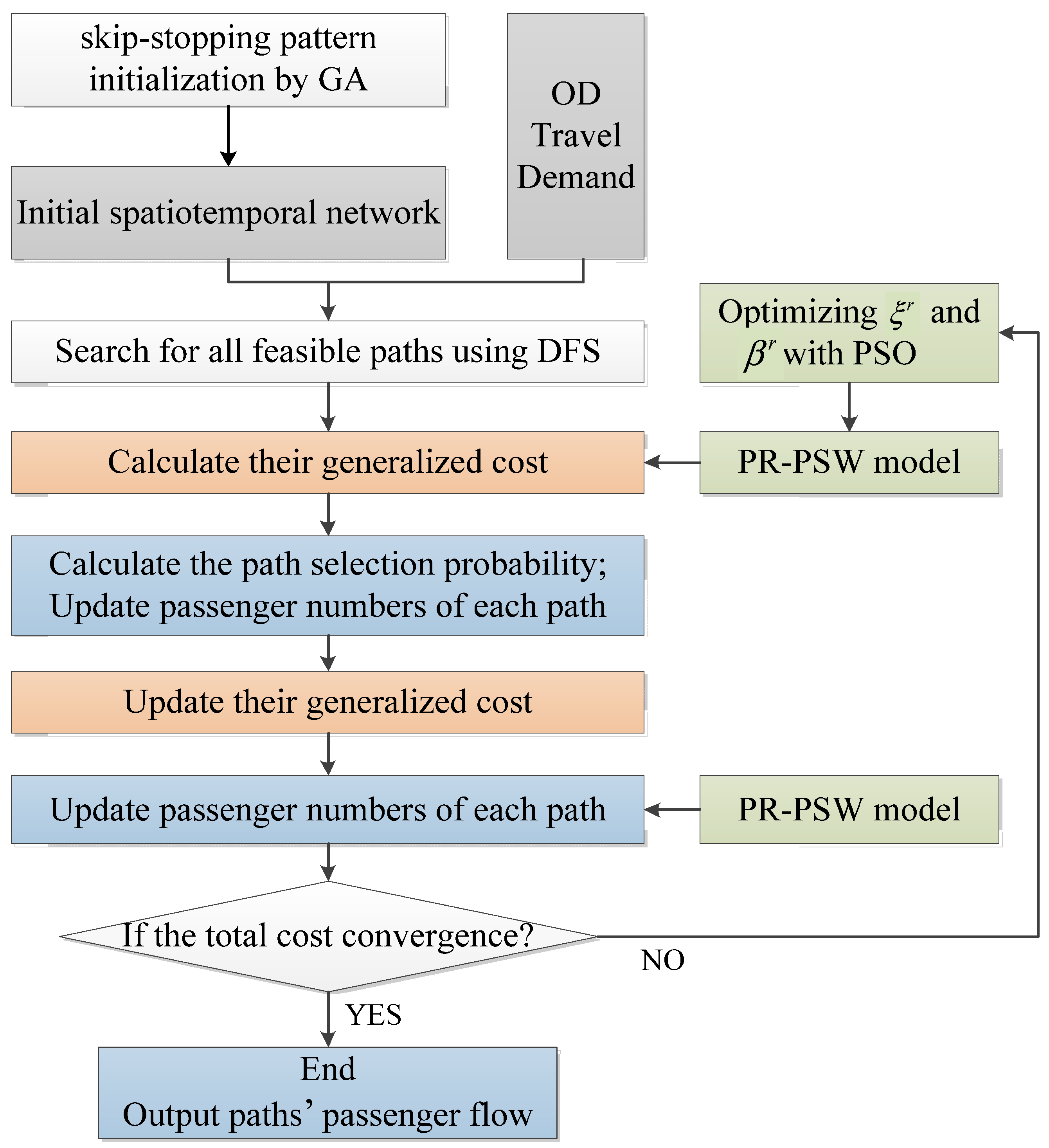
We employ the PR-PSW route choice model integrated with the PSO algorithm to assign multimodal passenger flow, and the flowchart of the solution algorithm is shown in Figure 3. In the proposed route choice model, as presented in Equation (20), there are two undetermined parameters that need to be calibrated: the shape parameter ${\xi }^r$ and the location parameter ${\beta }^r$ of the Weibull distribution. Since the selection of parameter values directly influences the passenger flow assignment results, we utilize the PSO algorithm to optimize these two parameters during the solution process of the assignment model, thereby determining the optimal parameter combination.

6. Timetable Adjustment

6.1. Interval Many-Objective Mixed Programming Model

The parameters used in Section 6 are shown in

Table 2. Model parameters and variables.

Notations	Description
Decision Variables
$\mathrm{\Delta }{T}_n^{Arrival}$	Adjustment time of train $n$’s arrival time (s)
$b_{ns}$	Whether train $n$ stop at station $s$
Variables
$T_{total}$	Total travel time interval (min)
$T_{total}^{Wait}$	Total wait time interval (min)
$T_{total}^{Adj}$	Total adjustment time (min)
$Nu{m}_{Dwell}^{Adj}$	Number of dwell status adjustments
$T_{d_j}^{Arrival after}$	Arrival time of passenger $j$’s train at destination station after adjustment
$T_{o_j}^{Depart after}$	Departure time of passenger $j$’s train at origin station after adjustment
$t_j^{Transfer}$	Transfer time of passenger $j$ (min)
$T_n^{Arrival after}$	Arrival time of train $n$ at destination station after adjustment
$T_{ns}^{Depart}$	Departure time of train $n$ at station $s$
$b_{njt}$	When passenger $j$ is on train $n$ at time $t$, values 1, otherwise 0
$T_{n_j^{trf after}{s}^{trf}}^{Depart}$	Departure time of train $n_j^{trf after}$ at transfer station $s^{trf}$
$T_{ns\prime }^{Dwell}$	Dwell time of train $n$ at station $s\prime$ (min)
Parameters
$t_j^{Arrival}$	Arrival time of passenger $j$ at origin station
$t_j^{Walk}$	Walk time of passenger $j$ (min)
$T_s^{Origin}$	Initial operation time of station $s$
$T_{nss\prime }^{Run}$	Run time of train $n$ from station $s$ to $s\prime$ (min)
$t_{j{s}^{trf}}^{Walk}$	Walk time of passenger $j$ at transfer station $s^{trf}$
$T_n^{am}$	Maximum time adjustment range of train $n$ (min)
${\prod }_{kp}^{remain-capacity}$	Remaining capacity at route $k$ of path $p$
$D_{s_j^{Origin}}$	Walking distance at origin station (m)
$V_j$	Walking speed of passenger $j$ (m/min)
$q_{ns}^{off}$	Getting off passengers for train $n$ at station $s$
$T_j^{wm}$	Maximum waiting time interval for passenger $j$ (min)

.

Objectives:

The objectives of minimizing passenger travel time, passenger waiting time, timetable adjustments, and stop pattern adjustments are formulated as shown in Equations (40), (41), (42), and (43), respectively.

$$\min T_{total}={\displaystyle \sum _{r\in R}{\displaystyle \sum _{p\in P}{\displaystyle \sum _{j=1}^{q_p^r}{T}_{d_j}^{Arrival after}-t_j^{Arrival}}}}$$

(36)

$$\min T_{total}^{Wait}={\displaystyle \sum _{r\in R}{\displaystyle \sum _{p\in P}{\displaystyle \sum _{j=1}^{q_p^r}{T}_{o_j}^{Depart after}-t_j^{Arrival}}}}+t_j^{Transfer}-t_j^{Walk}$$

(37)

$$\min T_{total}^{Adj}={\displaystyle \sum }_{n\in N}\left|T_n^{Arrival after}-T_n^{Arrival before}\right|$$

(38)

$$\min Nu{m}_{Dwell}^{Adj}={\displaystyle \sum }_{n\in N}{\displaystyle \sum _{s\in S}\left|b_{ns}^{After}-b_{ns}^{Before}\right|}$$

(39)

Due to the uncertainty of travel time and dwell time, we need to decide departure time and dwell status. At the same time, passengers may not board the expected train. Therefore, the wait time and travel time of passengers are dynamically changing with the timetable. The objectives (36) and (37) are to improve the passenger’s travel experience. Among them, the wait time includes the wait time at the origin station and at the transfer station. Travel time includes the entire travel time of passengers, not just time-in-vehicle.

Objective (38) represents the sum of the adjustment amounts for the departure time of each train at each station. Objective (39) represents the sum of the changes in dwell status for each train at each station. Both the number of stops that were originally stopped but now do not stop and the number of stops that were originally not stopped now are recorded as 1. These two objectives aim to achieve the goal of optimizing passenger experience with minimal train adjustments and achieving a dynamic balance between supply and demand.

Constraints:

(1)

The operational time constraints are formulated in Equations (40) and (41).

$$T_{ns}^{Depart}\ge T_s^{Origin}$$

(40)

$$T_{ns}^{Arrival}\le T_s^{Destination}$$

(41)

Departure time should be later than the earliest operation at the origin station, and the arrival time should be earlier than the latest operation at the terminal station.

(2)

The necessary travel time constraints are formulated in Equations (42) and (43).

$$T_{ns\prime }^{Arrival}-T_{ns}^{Departure}=T_{nss\prime }^{Run}\ge T_{nss\prime }^{Min}$$

(42)

Equation (42) requires that the travel time between two adjacent stations be greater than or equal to the minimum travel time $T_{nss\prime }^{Min}$. In addition, the travel time is an uncertain term, so combining this constraint with interval mathematics can be adjusted to Equation (43).

$$T_{ns\prime }^{Arrival}-T_{ns}^{Departure}\ge [T_{nss\prime }^{-},T_{nss\prime }^{+}]$$

(43)

(3)

The necessary headway constraints are formulated in Equations (44)–(50).

$$T_{n+1}^{Arrival after}-T_n^{Arrival after}\ge T_n^{stm},if b_{ns}^{track}=b_{\left(n+1\right)s}^{track},\forall n\in N,\forall s\in S$$

(44)

$$b_{ns}^{track}=\left\{\begin{array}{c}0, if n stops at s\\ 1, otherwise\end{array}\right.,\forall n\in N,\forall s\in S$$

(45)

$$T_{n+1}^{Arrival after}-T_n^{Arrival after}\ge [T_n^{st{m}^{-}},T_n^{st{m}^{+}}],if b_{ns}^{track}=b_{\left(n+1\right)s}^{track},\forall n\in N,\forall s\in S$$

(46)

$$T_{(n+1)s}^{Depart after}+T_{(n+1)ss\prime }^{Run}-T_{ns\prime }^{Depart after}\ge T_{s\prime }^{fm},if b_{ns}^{track}\ne b_{\left(n+1\right)s}^{track},\forall n\in N,\forall s\in S$$

(47)

$$T_{ns}^{Depart after}+T_{ns{s}^{\prime }}^{Run}-T_{(n-1)s\prime }^{Depart after}\ge T_{s\prime }^{fm},if b_{ns}^{track}\ne b_{\left(n-1\right)s}^{track},\forall n\in N,\forall s\in S$$

(48)

$$T_{(n+1)s}^{Depart after}+T_{(n+1)ss\prime }^{Run}-T_{ns\prime }^{Depart after}\ge [T_{s\prime }^{f{m}^{-}},T_{s\prime }^{f{m}^{+}}],if b_{ns}^{track}\ne b_{\left(n+1\right)s}^{track},\forall n\in N$$

(49)

$$T_{ns}^{Depart after}+T_{nss\prime }^{Run}-T_{(n-1)s\prime }^{Depart after}\ge [T_{s\prime }^{f{m}^{-}},T_{s\prime }^{f{m}^{+}}],if b_{ns}^{track}\ne b_{\left(n-1\right)s}^{track},\forall n\in N$$

(50)

Constraint (44) indicates that the minimum safety interval should be maintained between front and rear vehicles traveling on the same track. Formula (45) imposes constraints on track allocation. Considering that the minimum safety interval is an uncertain value, this constraint can be converted into Equation (46). Constraint (47) and (48) indicate that the arrival time of trains stopping at the same station and trains passing before/after different tracks should maintain a safe interval. Considering that the arrival interval is an uncertain value, combined with interval mathematics, constraint (47) and (48) can be converted into Formulas (49) and (50).

(4)

The overtaking constraint is formulated in Equation (51).

$$T_{ns\prime }^{Arrival after}+T_{ns\prime }^{Dwell}-T_{ns\prime }^{fm}\ge T_{(n+1)s}^{Depart after}+T_{(n+1)ss\prime }^{Run},if b_{ns}^{track}\ne b_{\left(n+1\right)s}^{track},\forall n\in N,\forall s\in S$$

(51)

We allow overtaking behavior at stations and set necessary arrival/departure intervals to prevent trains belonging to the same track/line from scheduling in a short period of time.

(5)

The path feasibility constraint is formulated in Equation (52).

$${\displaystyle \sum }_{j\in J}{T}_{pj}^{Wait}\ge 0,\forall p\in P,\forall j\in q_p^r$$

(52)

The wait time for passengers on each feasible path should not be less than 0, so that passengers on the assigned path will not miss the train.

(6)

The boarding status constraint is formulated in Equation (53).

$${\displaystyle \sum }_{n\in N}{b}_{njt}\le 1,\forall j\in J,\forall t\in T$$

(53)

When $b_{njt}=1$, passenger $j$ is in a vehicle at time $t$ and cannot take other trains.

(7)

The capacity constraints are formulated in Equations (54) and (55).

$${\displaystyle \sum }_{j\in J}{b}_{njt}\le M_n, \forall n\in N, \forall t\in T$$

(54)

$${\displaystyle \sum _{j=1}^{q_p^r}{b}_{njt}\le {\prod }_{kp}^{remain-capacity}, \forall n\in N, \forall t\in T,k=[s,s^{\prime }]}\in p$$

(55)

These two constraints indicate that the sum of the on-board states of all passengers at time $t$ should be less than the total capacity of the train, while the sum of the on-board states of all passengers who have not boarded at time $t$ should be less than the remaining capacity of the train.

(8)

The transfer constraints are formulated in Equations (56)–(58).

$$T_{n_j^{trf after}{s}^{trf}}^{Depart}\ge T_{n_j^{trf before}{s}^{trf}}^{Arrival}+t_{j{s}^{trf}}^{Walk},\forall j\in \left\{j|b_{njt}=1\right\},\forall s^{trf}\in S$$

(56)

$$t_{j{s}^{trf}}^{Wait}=T_{n_j^{trf after}{s}^{trf}}^{Depart}-T_{n_j^{trf before}{s}^{trf}}^{Arrival}-t_{j{s}^{trf}}^{Walk},\forall j\in \left\{j|b_{njt}=1\right\},\forall s^{trf}\in S$$

(57)

$$t_{j{s}^{trf}}^{Walk}=D_{n_j^{trf before}}^{n_j^{trf after}}/V_j$$

(58)

Constraint (56) is a transfer time constraint, indicating that the boarding time for passengers after a transfer must be later than getting off the previous train and walking to the boarding platform.

(9)

The dwell constraints are formulated in Equations (59)–(63).

$$T_{ns}^{Dwell}=T_{ns}^{Depart}-T_{ns}^{Arrival}$$

(59)

$$T_{ns}^{D_{\min }}\le T_{ns}^{Depart}-T_{ns}^{Arrival}\le T_{ns}^{D_{\max }}$$

(60)

$$[T_{ns}^{D_{min}^{-}},T_{ns}^{D_{min}^{+}}]\le T_{ns}^{Depart}-T_{ns}^{Arrival}\le [T_{ns}^{D_{max}^{-}},T_{ns}^{D_{max}^{+}}]$$

(61)

$$T_{ns}^{D_{\min }}\ge {\displaystyle \frac{{(m_n\rho )}^{m_n}{P}_0\times q_{ns}^{off}}{\mu \times {\left(1-\rho \right)}^2\times m_n!}}$$

(62)

$$b_{ns}=\left\{\begin{array}{c}1, if n stops at s\\ 0, otherwise\end{array}\right.,\forall n\in N,\forall s\in S$$

(63)

The dwell time of train $n$ at station $s$ is a threshold, but the upper and lower bounds of the threshold are uncertain and can change due to dynamic passenger flow and other factors. Combined with interval mathematics, constraint (60) can be transformed into Equation (61). In addition, the dwell time also needs to meet passengers’ boarding and alighting needs. Dwell status $b_{ns}$ is a Boolean variable.

(10)

The wait time constraints are formulated in Equations (64)–(67).

$$T_{{n_j{s}_j}^{Origin}}^{Depart}\ge t_j^{Arrival}+t_{j{s}_j^{Origin}}^{Walk},\forall j\in \left\{j|b_{njt}=0\right\},\forall s_j^{Origin}\in S$$

(64)

$$t_{j{s}_j^{Origin}}^{Wait}=T_{n_j{s}_j^{Origin}}^{Depart}-t_j^{Arrival}-t_{j{s}_j^{Origin}}^{Walk},\forall j\in \left\{j|b_{njt}=0\right\},\forall s_j^{Origin}\in S$$

(65)

$$t_{j{s}_j^{Origin}}^{Walk}=D_{s_j^{Origin}}/V_j$$

(66)

$$t_{j{s}_j^{Origin}}^{Wait}\le T_j^{wm},\forall j\in J$$

(67)

Similar to the transfer constraint (56), the wait time of passenger $j$ at the origin station is defined by constraint (65), ensuring that passengers can board the train according to the assigned path. At the same time, constraint (67) defines the maximum wait time, which is closer to passengers’ actual choice.

(11)

The adjustment range constraints are formulated in Equations (68) and (69).

$$\left|T_n^{Arrival after}-T_n^{Arrival before}\right|=\mathrm{\Delta }{T}_n^{Arrival}\le T_n^{am}, \forall n\in N$$

(68)

Equation (68) constrains the time adjustment margin, which can be set by considering a combination of the magnitude of adjustment and the degree of impact on other stations. Introducing interval mathematics, this constraint can be transformed into Equation (69).

$$\left|T_n^{Arrival after}-T_n^{Arrival before}\right|\le [T_n^{a{m}^{-}},T_n^{a{m}^{+}}], \forall n\in N$$

(69)

6.2. Model Solving

In order to determine the optimal value of the uncertainty and obtain timetable optimization schemes, the model is solved by IMOEA-MC. The solving steps are shown in Algorithm 1.

Algorithm 1: Procedure of IMOEA-MC
	Input $NP$, population size; $MAX\_FES$, maximum function evaluations;
	Output $P_{g+1}$, the nondominated population;
1	Initialize an initial population $P_g=Intialization\left( \right),g=0$
2	$for g=1:Max\_FES:$
3	$Q_g=Recombination+Mutation(P_g)$
4	$R_g=P_g{\displaystyle \cup Q_g}$//Combine parent and offspring population
5	$\left\{F_1,F_2,\dots \right\}=nondominated-sort(Q_{g+1})$//All nondominated fronts of $R_g$
6	$P_{g+1}=Ø, i=1$
7	Until $\left|P_{g+1}\right|+\left|F_i\right|<NP$
	//Optimal Solution Sorting Based on Reference Polyhedron.
8	$RP=Construct Reference Polyhedron(F_i)$
9	$Sort(F_i,\mathrm{Integrated} \prec n)$
10	$P_{g+1}=P_{g+1}{\displaystyle \cup F_i}$
11	$i=i+1$
12	$P_{g+1}=P_{g+1}{\displaystyle \cup F_i}\left[1:\left(NP-\left|P_{g+1}\right|\right)\right]$//Choose the first $\left(NP-\left|P_{g+1}\right|\right)$ elements of       $F_i$
13	$g=g+1$
14	$end for$

The algorithm needs to sample each interval value based on the Monte Carlo method to further develop rich scenarios and obtain more robust schedules. Specifically, it is reflected in the generation and combination of the population, which requires the combination of different interval values.

The specific steps for the 8th and 9th lines in Algorithm 1 are as follows.

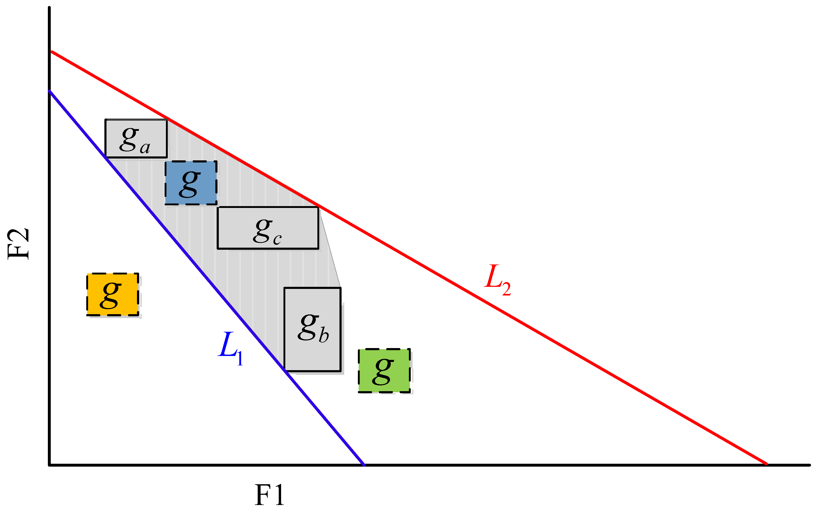
Step1: Select the best, worst, and the recent interval solutions $g_a,g_b,g_c$ from the solution set.

Step2: Connect the bottom left corner of $g_a$ and $g_b$, and the top right corner of $g_a$ and $g_c$, calculate the slope of two straight lines $L_1$ and $L_2$.

Step3: Construct a Reference Polyhedron with $g_a,g_b,g_c$ as fixed points and $L_1$,$L_2$ as edges.

Step4: Sort each individual in the same $F_i$ using Reference Polyhedron-based dominance relationships.

(1)

Inside the polyhedron, the sorting is optimal.

(2)

Outside the range composed of $L_1$ and $L_2$, sort in the middle.

(3)

Under the polyhedron, the sorting is the worst.

We use Figure 4 to describe the above process. As illustrated in Figure 4, the grey area represents the constructed reference polyhedron. Based on this polyhedron, the solutions in the objective space can be divided into three categories. First, solutions located inside the reference polyhedron, denoted by the blue boxes, exhibit a balanced performance across multiple objectives and are assigned the highest sorting priority. Second, solutions located under the reference polyhedron, represented by the green boxes, possess at least one objective value worse than the worst-case solution, thus receiving the lowest sorting priority. Finally, solutions located outside the region bounded by the reference lines and axes, indicated by the orange boxes, have an intermediate sorting priority that falls between the aforementioned two cases.

7. Computational Experiments

In order to verify the performance of the proposed two-stage model and solving algorithms, we selected intercity transportation networks (Beijing–Zhangjiakou, Chengdu–Chongqing, Guangzhou–Qingyuan) from three different urban agglomerations for validation. These three intercity road networks are located in Northern, Southwestern, and Southern China, respectively, covering a wide geographical range. Meanwhile, Beijing and Chongqing are municipalities directly under the Central Government. Therefore, these three networks possess a certain degree of representativeness. This study focuses exclusively on optimizing transportation modes with fixed schedules, specifically High-speed Rail, EMU, Ordinary Rail, and Coach. Simultaneously, the OD passenger flow is aggregated into 60 min intervals to serve as the demand input for timetable optimization. Specifically, the corresponding train timetable data were derived from actual public data on the official 12306 platform, while the total OD passenger volume was referenced from the statistical yearbooks of the respective provinces and cities. The experimental environment is as follows: Lenovo PC (Lenovo, Beijing, China) with Intel processor ^® Core (TM) i7-10700 CPU @ 2.90GHz, RAM is 16 GB. The software version is PyCharm 2020.3.2.

We set the population size to 40 and the number of iterations to 2000. We use simulated binary crossover for real and int types, use half uniform crossover for bool type, and set the crossover rate to 0.8. Moreover, we use polynomial mutation for real and int types, use bitflip mutation for bool type, and set the mutation rate to 0.2.

7.1. Passenger Flow Assignment

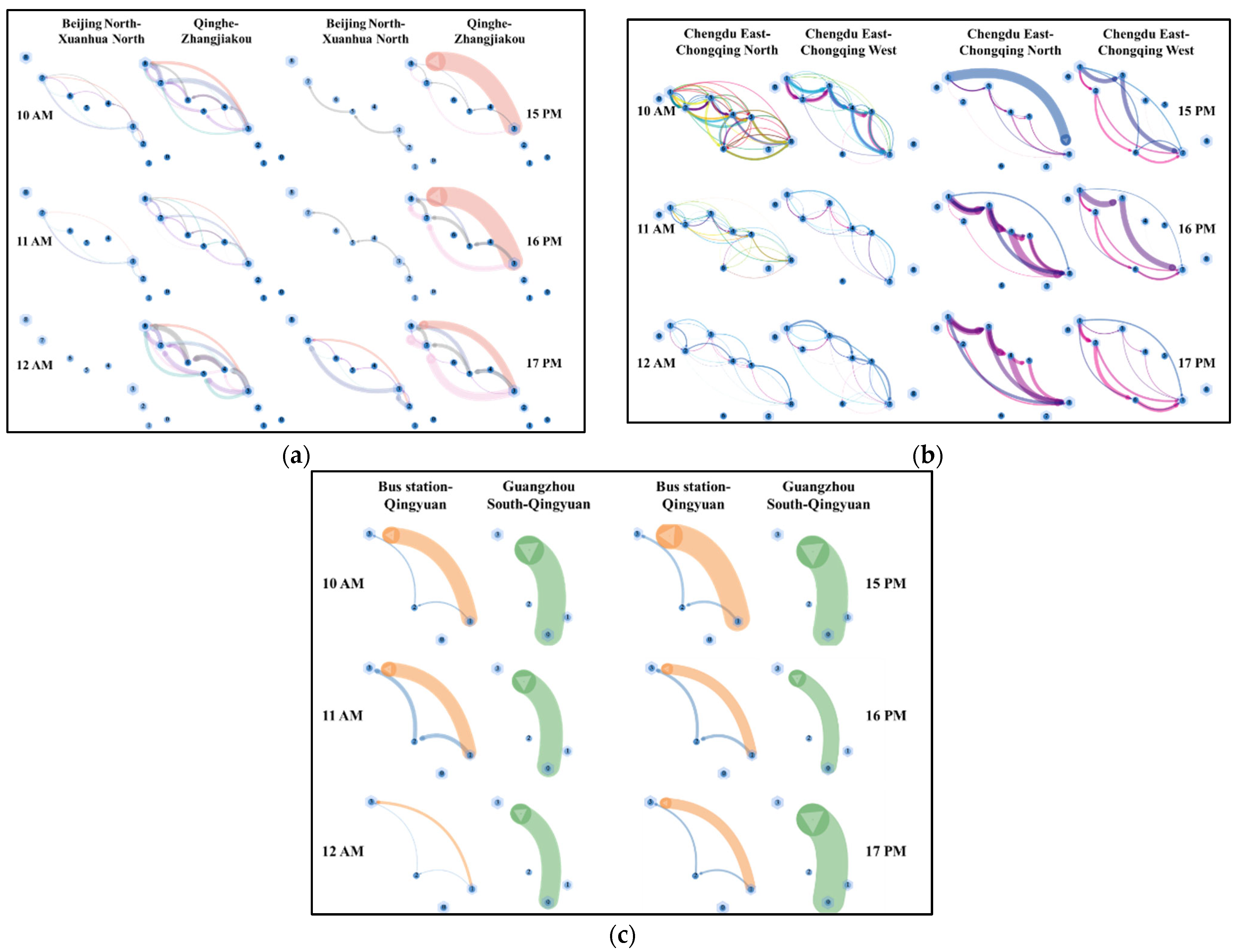
We validated three time periods for each AM and PM of the day, totaling six hours. Figure 5 shows the passenger flow allocation results for different paths in the six time periods.

It can be seen from Figure 5 that the feasible paths of the same network change at different times. The blue dots in the figure represent different transit hubs. Taking Figure 5a as an example, the nodes from 0 to 8 are Bus Station, Beijing Fengtai, Beijingbei, Qinghe, Donghuayuanbei, Huailai, Xiahuayuanbei, Xuanhuabei, and Zhangjiakou station, respectively. Different color lines indicate different paths, and the width of the line indicates the flow. The wider the line, the greater the flow. It can be seen that the feasible path for OD pair 1 (Beijingbei–Xuanhuabei) is much less than that for OD pair 2 (Qinghe–Zhangjiakou), and the demand for OD 1 is also much lower, which is consistent with the actual situation. Except for 15 PM and 16 PM, the flow distribution is relatively balanced. The reason is that the cost of the non-transfer routes from Qinghe to Zhangjiakou for 15 PM and 16 PM are much lower than the cost of the required transfer routes, which is also in line with the true travel choices of passengers. Figure 5b,c are the same as Figure 5a, but in order to save space, there will be no more explanation here.

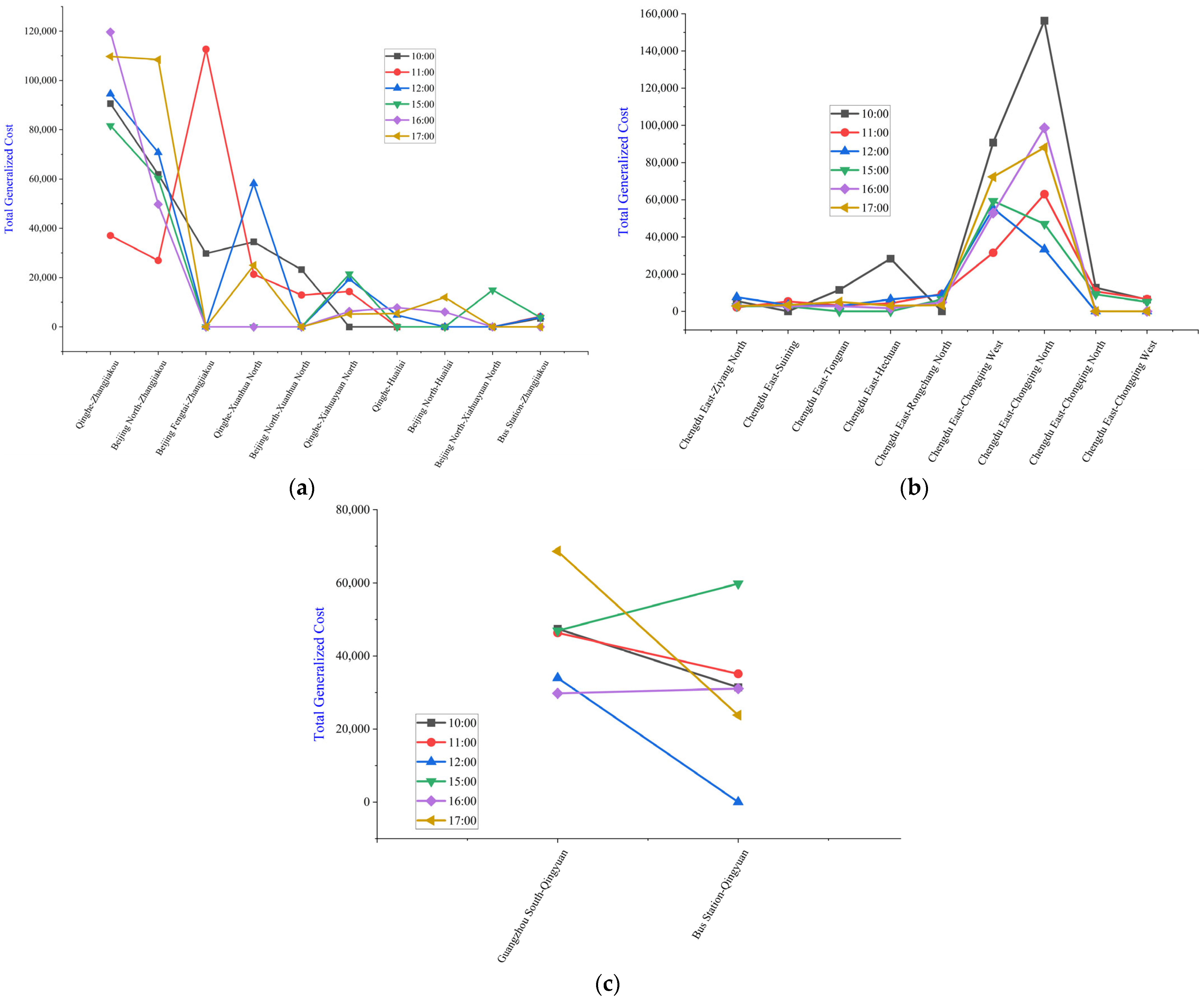
The objective of passenger flow assignment is minimizing the total generalized cost of the system. As a supplement, Figure 6 shows the total generalized cost of the system for different OD pairs, i.e., different paths at different times corresponding to the optimal solution of the first stage model.

It can be seen that the generalized cost of OD pairs is closely related to passenger flow. For example, by comparing Figure 5a and Figure 6a, we can see that the passenger flow from Qinghe to Zhangjiakou at 16 PM is significantly greater than that at 11 AM, so the generalized cost value is also significantly larger.

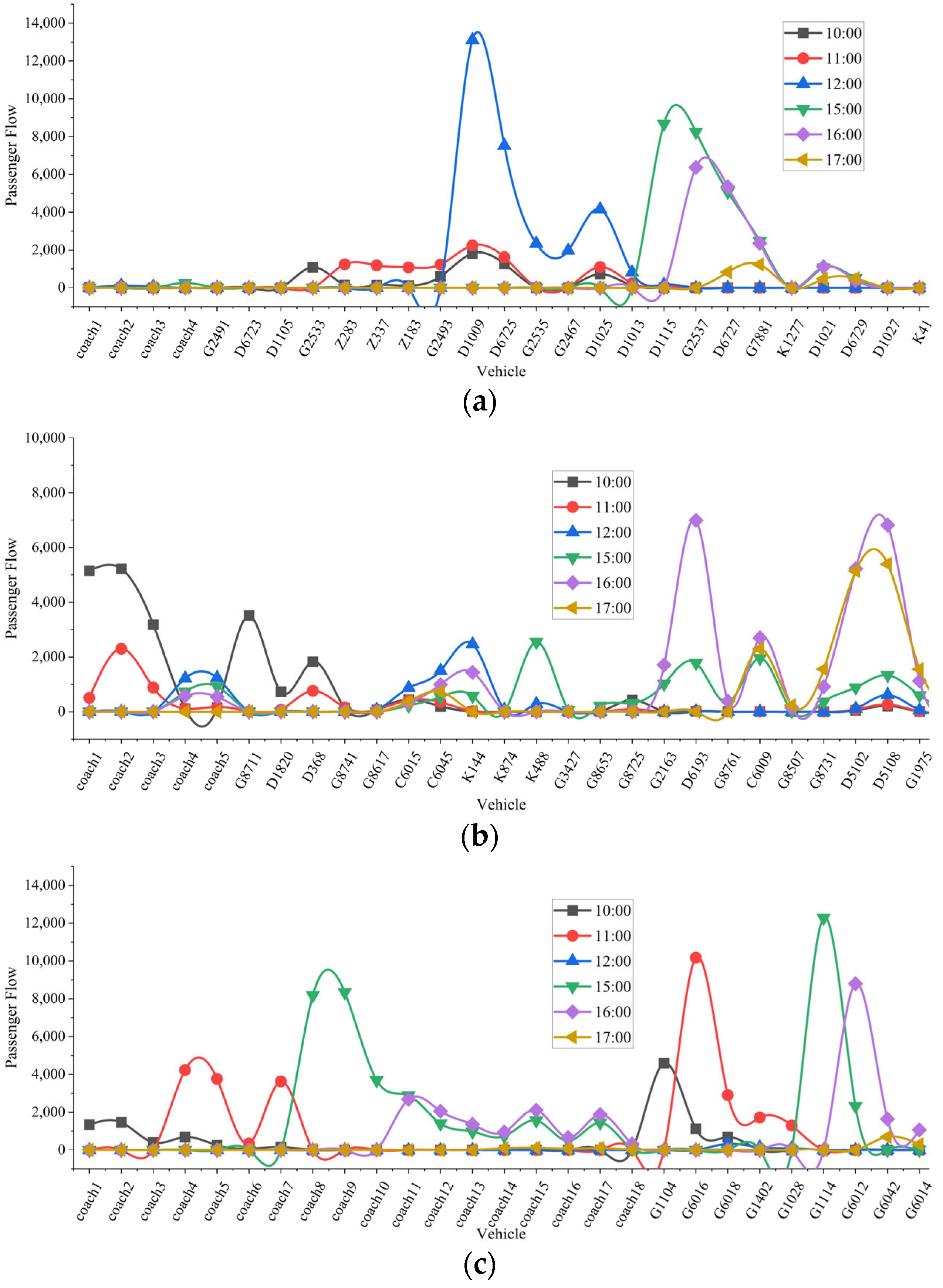
In addition, it should be noted that there are several routes that can serve the same OD pair. It should also be noted that on the same road section, such as Qinghe to Xuanhua North, there are many vehicles that can pass, such as G2533, G2493, and D1009, etc. The passenger flow of each vehicle is the sum of the flow of all paths including the vehicle. It is shown in Figure 7.

From Figure 7, we can see that the passenger flow of some vehicles is significantly higher, or it exceeds the capacity of the vehicle, which is also common in real life. For these passengers, we set penalties for exceeding capacity and include them in the objective function for further optimization. Of course, this result also provides guidance for operation planning, where passengers can choose more time and vehicles for planning, such as increasing vehicles, to maximize overall service efficiency.

7.2. Timetable Optimization

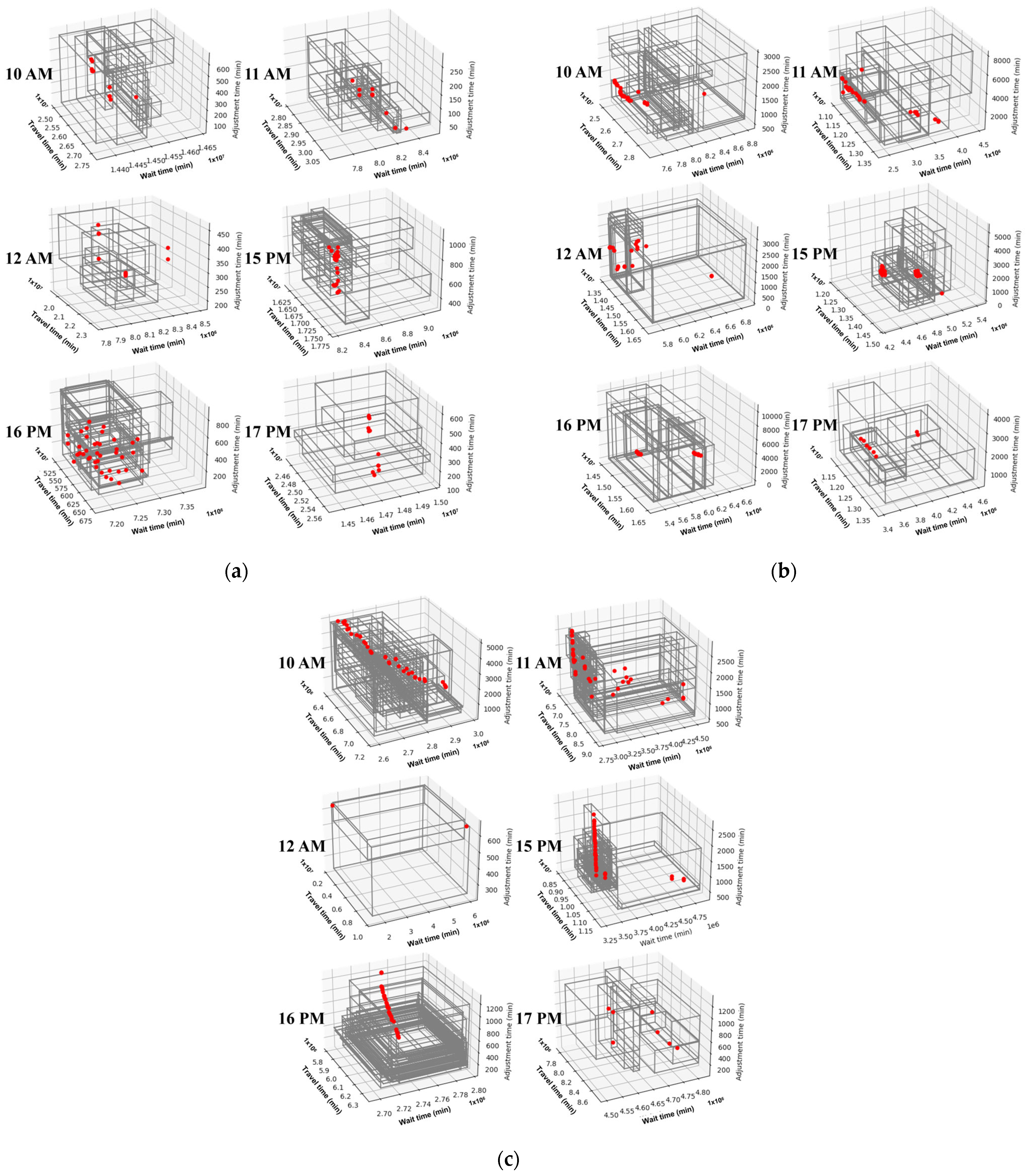
The robustness of the proposed IMOEA-MC algorithm was evaluated in comparison with NSGA-II. Figure 8 shows the comparison results of objective functions. For the convenience of display, we selected F1, F2, and F3 as the x-axis, y-axis, and z-axis to draw a three-dimensional scatter plot.

In Figure 8, the gray cube represents the interval solution obtained by the IMOEA-MC algorithm, while the red dots represent the optimal solution obtained by the NSGA-II algorithm. It can be seen that the number of solutions varies in different datasets and different times. For example, in Figure 8c, only two solutions are obtained, indicating that there are only two feasible solutions in this scenario. On this basis, it can be clearly seen that the cube has good encapsulation for the red dots, indicating that the interval solution achieves the purpose of preserving uncertainty in the solving process. In addition, it also indicates that there are better solutions in the interval solution than the solutions solved by NSGA-II. Thus, the diversity of the solution set is better, there are more selectable solutions, the scenarios are richer, and the optimized timetables are more robust. Taking 10 AM in Figure 8c as an example, the maximum difference between the F1 value in the interval solution and the value obtained by NSGA-II is 776,110.19, decreases 12.15%. The difference of F2 is 221,041.3, decreases 8.53%. The difference of F3 is 7, decreases 36.84%. The difference of F4 is 3346 s, decreases 84.82%. In addition to solution quality, the proposed method demonstrates good adaptability to the studied network. The computation time for optimizing an hourly passenger flow scenario is consistently controlled within 1000 s.

In order to assess the merits of the solution set and select the optimal, we use the pseudo-weight vector method [35] to calculate the pseudo-weight vector for each non-dominated solution and select the solution corresponding to the weight vector that is closest to the decision maker’s subjective preference. We select two timing points, and the corresponding optimal solutions are shown in

Table 3. Optimized timetable solved by IMOEA-MC at 12 AM.

Beijing-Zhangjiakou			Chengdu-Chongqing			Guangzhou-Qingyuan
ID	Initial	Optimized	ID	Initial	Optimized	ID	Initial	Optimized
coach1	10:40	10:42	coach1	10:00	10:01	coach1	10:00	10:00
coach2	13:30	13:30	coach2	11:00	11:00	coach2	10:10	10:14
coach3	14:10	14:10	coach3	11:30	11:30	coach3	10:30	10:30
coach4	16:00	16:01	coach4	15:00	15:02	coach4	10:50	10:50
G2491	8:31	8:31	coach5	15:30	15:30	coach5	11:00	11:00
D6723	8:50	8:50	G8711	10:05	10:05	coach6	11:55	11:55
D1105	9:15	9:15	D1820	10:13	10:14	coach7	12:00	12:00
G2533	10:32	10:32	D368	10:53	10:53	coach8	15:00	15:00
Z283	11:23	11:23	G8741	11:38	11:38	coach9	15:10	15:10
Z337	11:30	11:30	G8617	12:26	12:26	coach10	15:40	15:40
Z183	11:40	11:40	C6015	12:43	12:43	coach11	16:00	16:00
G2493	12:00	12:00	C6045	13:14	13:14	coach12	16:15	16:15
D1009	12:06	12:06	K144	14:01	14:18	coach13	16:30	16:34
D6725	12:29	12:29	K874	14:13	14:13	coach14	16:50	16:50
G2535	13:00	13:00	K488	15:00	15:00	coach15	17:10	17:10
G2467	13:15	13:15	G3427	15:21	15:21	coach16	17:30	17:31
D1025	13:58	13:58	G8653	15:31	15:32	coach17	17:35	17:35
D1013	14:47	14:48	G8725	15:47	15:47	coach18	18:00	18:00
D1115	15:06	15:06	G2163	16:03	16:03	G1104	10:30	10:30
G2537	16:05	16:05	D6193	16:11	16:11	G6016	11:41	11:41
D6727	17:25	17:25	G8761	16:46	16:46	G6018	12:33	12:33
G7881	19:05	19:05	C6009	16:56	16:56	G1402	13:00	13:00
K1277	19:17	19:17	G8507	17:06	17:06	G1028	13:17	13:17
D1021	19:52	19:52	G8731	17:16	17:16	G1114	15:16	15:18
D6729	20:35	20:35	D5102	17:30	17:32	G6012	16:43	16:43
D1027	20:41	20:41	D5108	17:52	17:52	G6042	18:00	18:00
K41	20:45	20:45	G1975	18:35	18:36	G6014	18:32	18:32
			G8661	18:57	18:58

and

Table 4. Optimized timetable solved by IMOEA-MC at 16 PM.

Beijing-Zhangjiakou			Chengdu-Chongqing			Guangzhou-Qingyuan
ID	Initial	Optimized	ID	Initial	Optimized	ID	Initial	Optimized
coach1	10:40	10:40	coach1	10:00		coach1	10:00	10:00
coach2	13:30	13:30	coach2	11:00	11:01	coach2	10:10	10:10
coach3	14:10	14:10	coach3	11:30	11:33	coach3	10:30	10:30
coach4	16:00	16:00	coach4	15:00		coach4	10:50	10:50
G2491	8:31	8:31	coach5	15:30		coach5	11:00	11:00
D6723	8:50	8:50	G8711	10:05		coach6	11:55	11:55
D1105	9:15	9:15	D1820	10:13		coach7	12:00	12:00
G2533	10:32	10:32	D368	10:53		coach8	15:00	15:00
Z283	11:23	11:23	G8741	11:38	11:39	coach9	15:10	15:10
Z337	11:30	11:30	G8617	12:26		coach10	15:40	15:40
Z183	11:40	11:40	C6015	12:43		coach11	16:00	16:00
G2493	12:00	12:01	C6045	13:14	13:22	coach12	16:15	16:15
D1009	12:06	12:06	K144	14:01		coach13	16:30	16:30
D6725	12:29	12:29	K874	14:13		coach14	16:50	16:50
G2535	13:00	13:00	K488	15:00		coach15	17:10	17:10
G2467	13:15	13:15	G3427	15:21	15:22	coach16	17:30	17:30
D1025	13:58	13:58	G8653	15:31		coach17	17:35	17:35
D1013	14:47	14:47	G8725	15:47		coach18	18:00	18:00
D1115	15:06	15:06	G2163	16:03		G1104	10:30	10:30
G2537	16:05	16:05	D6193	16:11		G6016	11:41	11:41
D6727	17:25	17:25	G8761	16:46	16:47	G6018	12:33	12:33
G7881	19:05	19:05	C6009	16:56		G1402	13:00	13:00
K1277	19:17	19:17	G8507	17:06		G1028	13:17	13:17
D1021	19:52	19:52	G8731	17:16		G1114	15:16	15:16
D6729	20:35	20:38	D5102	17:30		G6012	16:43	16:43
D1027	20:41	20:41	D5108	17:52	17:55	G6042	18:00	18:01
K41	20:45	20:45	G1975	18:35	18:38	G6014	18:32	18:33
			G8661	18:57	18:59

.

In above tables, the vehicles marked with different colors are the ones that need to adjust. It can be seen that this plan achieves an improvement in passenger service efficiency with fewer adjustments and improves the synergy between various transportation modes, too.

8. Discussion

The two-stage framework proposed in this study can effectively coordinate multimodal timetables and passenger flows under uncertain conditions, with a particular focus on developing robust timetables to enhance the synergy among different travel modes. By optimizing departure times and stopping patterns under uncertainty, the model achieves a dynamic balance between travel demand and transport supply, enabling passengers to flexibly choose combinations of modes and vehicles according to dynamic decisions. Furthermore, the two-stage structure significantly shrinks the search space of feasible solutions, while the proposed IMOEA-MC algorithm successfully preserves uncertainty information in practical applications. The case studies in three urban agglomerations confirm that the interval-based approach provides a set of diverse and implementable timetables. Compared with the deterministic NSGA-II solutions, the interval solutions better reflect uncertain parameters and demonstrate superior performance in terms of solution diversity and robustness.

Compared with existing studies, this research contributes in three aspects. First, distinct from single-mode studies assuming fixed demand, our model explicitly integrates multimodal path choice. The improved PR-PSW model addresses the heterogeneity of traditional Logit approaches, while the inclusion of virtual paths effectively manages capacity constraints to reflect realistic dynamic decision-making. Second, traditional robust or stochastic optimization methods usually transform uncertainty into a single expected objective, which may lose valuable information. The proposed interval many-objective framework keeps the range of possible outcomes and provides decision makers with richer alternatives. Third, the two-stage structure avoids the infeasibility and local optimum problems that often appear in iterative joint optimization and shows good performance on networks with different scales and service patterns.

Furthermore, the designed two-stage model has four advantages compared to the iterative method, including: (a) performing cross mutation on decision variables to ensure the search space capacity and solutions’ diversity, (b) using an improved passenger flow assignment algorithm to optimize passenger routing, (c) considering various uncertainties in timetable optimization, and (d) combining Monte Carlo algorithm with NSGA-II algorithm-based interval many-objective evolutionary algorithm to solve the timetable optimization model, ensuring scenes’ richness while improving the solutions’ convergence.

Nevertheless, several limitations should be acknowledged. Multimodal coordination in practice is constrained by institutional fragmentation and data silos among High-speed Rail, Ordinary Rail, and Coach operators. The proposed framework therefore does not assume full real-time data sharing; instead, it is designed as a planning-level approach based on information that is publicly accessible, such as published timetables, vehicle capacities, hub transfer relationships, and aggregated OD demand. However, achieving a higher level of real-time synergy ultimately requires overcoming these socio-technical barriers. Furthermore, the pursuit of personalized timetable optimization introduces critical ethical and privacy concerns. While granular passenger trajectory data can theoretically improve scheduling precision, it raises significant risks regarding surveillance and data misuse. Therefore, future research efforts need to balance model performance with passenger information protection.

9. Conclusions

This paper introduces a two-stage model for optimizing multimodal timetables in uncertain scenarios and proposes a corresponding solution algorithm to obtain a non-dominated solution set considering constraints such as time window and capacity. The first stage is the passenger flow assignment model, with the objectives of minimizing travel time, wait time, vehicles adjustment quantities, and adjustment time. The solving algorithm seeks the pareto solution set by preserving the uncertainty of actual problem as much as possible and enriching the its diversity.

We tested our algorithm on the Beijing–Zhangjiakou, Chengdu–Chongqing, and Guangzhou–Qingyuan intercity networks. Our verification result indicates that there is indeed a quantifiable interaction between passenger’s assignment and timetable. Passenger route choice is dynamic and responsive to timetable adjustments. Therefore, the proposed algorithm achieves a dynamic balance between travel demand and multimodal transportation service supply. Additionally, it is shown that the algorithm retains more uncertainty information and obtains better solutions, which performs well compared to NSGA-II in three cases under different origins and destinations. Specifically, taking the Guangzhou–Qingyuan network at 10 AM as an example, the maximum differences in the interval solutions of the proposed method compared to NSGA-II for objectives F1, F2, F3, and F4 were 776,110.19 (a 12.15% decrease), 221,041.3 (an 8.53% decrease), 7 (a 36.84% decrease), and 3346 s (an 84.82% decrease), respectively. This indicates that the proposed interval solutions contain superior alternatives to NSGA-II, demonstrating better diversity of the solution set, more selectable alternatives, and lower uncertainty. In the future, with the support of data, we will conduct research and verification under a large-scale network of three or more cities and further optimize passengers’ experience by optimizing multimodal timetables. Simultaneously, we will utilize real-world data to calibrate the interval parameter boundaries, thereby enhancing the model’s precision.

References

1. Qi, W.; Yu, L.; Tang, X.; Wu, J.; Zhang, Y.; He, Z. Multi-objective optimization of a hydrogen-fueled PEMFC with multi wavy channels via machine learning and CFD simulation. Int. J. Hydrogen Energy 2026, 199, 152748. [Google Scholar] [CrossRef]
2. Qi, W.; Yu, J.; Wang, X.; Zhang, R.; Wu, X.; Xue, S.; Yang, J.; Ge, S.; Zhang, Y.; He, Z. Thermal management performance enhancement of cylindrical power battery modules via cooling strips with reflux microchannel structure. Energy 2026, 346, 140312. [Google Scholar] [CrossRef]
3. Macioszek, E.; Granà, A.; Fernandes, P.; Coelho, M.C. New Perspectives and Challenges in Traffic and Transportation Engineering Supporting Energy Saving in Smart Cities—A Multidisciplinary Approach to a Global Problem. Energies 2022, 15, 4191. [Google Scholar] [CrossRef]
4. Wang, X.; Tian, J.; Liu, E. Enhancing the Resilience of Intercity Transit System by Integrated Multimodal Emergency Dispatching and Passenger Assignment. Sustainability 2025, 17, 5717. [Google Scholar] [CrossRef]
5. Zhu, Y.; Goverde, R.M. Dynamic and robust timetable rescheduling for uncertain railway disruptions. J. Rail Transp. Plan. Manag. 2020, 15, 100196. [Google Scholar] [CrossRef]
6. Huang, Z.; Zheng, H. Integrated Line Planning and Timetable Scheduling for Railways Considering the Dynamics and Uncertainty of Passenger Demand. IET Intell. Transp. Syst. 2025, 19, e70019. [Google Scholar] [CrossRef]
7. Schöbel, A. An eigenmodel for iterative line planning, timetabling and vehicle scheduling in public transportation. Transp. Res. Part C Emerg. Technol. 2017, 74, 348–365. [Google Scholar] [CrossRef]
8. Xie, J.; Zhan, S.; Wong, S.C.; Lo, S.M. A schedule-based timetable model for congested transit networks. Transp. Res. Part C Emerg. Technol. 2021, 124, 102925. [Google Scholar] [CrossRef]
9. Chen, Y.Z.; Shi, C.L.; Claudel, C.G.; Hu, M.B. First train timetable synchronization with interval trains in subway networks. Transp. B Transp. Dyn. 2023, 11, 69–92. [Google Scholar] [CrossRef]
10. Li, J.; Zhang, L.; Liu, B.; Shi, N.; Li, L.; Yin, H. Travel-Energy-Based Timetable Optimization in Urban Subway Systems. Sustainability 2023, 15, 1930. [Google Scholar] [CrossRef]
11. Du, Y.; Ye, X.; Chen, D.; Ni, S. Last-train timetable synchronization for service compatibility maximization in urban rail transit networks with arrival uncertainties. Appl. Math. Model. 2025, 138, 115768. [Google Scholar] [CrossRef]
12. Zhang, J.; Zhang, Z.; Cai, X.; Cai, J.; Chen, J. An interval evolutionary algorithm based on dynamic relation adjustment strategy for many-objective problems. Swarm Evol. Comput. 2025, 93, 101853. [Google Scholar] [CrossRef]
13. Cai, J.; Chen, B.; Zhang, M.; Wen, J.; Cui, Z.; Chen, J. A Fairness-Aware Resource Management Model With Many-Objective Optimization in Uncertain Resource-Constrained Internet of Vehicles. IEEE Internet Things J. 2025, 12, 26718–26729. [Google Scholar] [CrossRef]
14. Sun, J.; Miao, Z.; Gong, D.; Zeng, X.; Li, J.; Wang, G. Interval multi-objective optimization with memetic algorithms. IEEE Trans. Cybern. 2020, 50, 3444–3457. [Google Scholar] [CrossRef] [PubMed]
15. Wang, B.; Zhang, C.; Li, C.; Li, P.; Dong, Z.; Lu, J. Hybrid interval-robust adaptive battery energy storage system dispatch with SOC interval management for unbalanced microgrids. IEEE Trans. Sustain. Energy 2022, 13, 44–55. [Google Scholar] [CrossRef]
16. Chen, Y.; Chan, W.H.; Su, E.L.M.; Diao, Q. Multi-objective optimization for smart cities: A systematic review of algorithms, challenges, and future directions. PeerJ Comput. Sci. 2025, 11, e3042. [Google Scholar] [CrossRef]
17. Deb, K.; Lopes, C.L.d.V.; Martins, F.V.C.; Wanner, E.F. Identifying Pareto Fronts Reliably Using a Multistage Reference-Vector-Based Framework. IEEE Trans. Evol. Comput. 2024, 28, 252–266. [Google Scholar] [CrossRef]
18. Guo, X.; Wu, J.; Sun, H.; Yang, X.; Jin, J.G.; Wang, D.Z.W. Scheduling synchronization in urban rail transit networks: Trade-offs between transfer passenger and last train operation. Transp. Res. Part A Policy Pract. 2020, 138, 463–490. [Google Scholar] [CrossRef]
19. Shen, X.; Lou, H.; Ge, Z. A two-stage scheduling algorithm for dynamic interval multi-objective vehicle routing problem in medical waste collection. Comput. Ind. Eng. 2025, 205, 111136. [Google Scholar] [CrossRef]
20. Liu, W.; Fu, M.; Yang, M.; Yang, Y.; Wang, L.; Wang, R.; Zhao, T. A bi-level interval robust optimization model for service restoration in flexible distribution networks. IEEE Trans. Power Syst. 2021, 36, 1843–1855. [Google Scholar] [CrossRef]
21. Wei, F.; Qin, S.; Feng, G.; Sun, Y.; Wang, J.; Liang, Y. Hybrid model-data driven network slice reconfiguration by exploiting prediction interval and robust optimization. IEEE Trans. Netw. Serv. Manag. 2022, 19, 1426–1441. [Google Scholar] [CrossRef]
22. Yi, J.; Bai, J.; He, H.; Zhou, W.; Yao, L. A multifactorial evolutionary algorithm for multitasking under interval uncertainties. IEEE Trans. Evol. Comput. 2020, 24, 908–922. [Google Scholar] [CrossRef]
23. Xu, Y.; Pi, D.; Yang, S.; Chen, Y.; Qin, S.; Zio, E. An angle-based bi-objective optimization algorithm for redundancy allocation in presence of interval uncertainty. IEEE Trans. Autom. Sci. Eng. 2023, 20, 271–284. [Google Scholar] [CrossRef]
24. Zhang, R.J.; Yang, M.; Wang, Y.C.; Ye, M.; Zou, J.; Pan, Z.Y. Dual-Objective Timetabling Method for Urban Rail Transit with Varying Express/Local Ratios. Transp. Res. Rec. 2025, 03611981251394966. [Google Scholar] [CrossRef]
25. Zhao, Q.; Tang, J.; Zhang, X. Collaborative passenger flow control for an urban rail transit network. Comput. Aided Civ. Infrastruct. Eng. 2024, 39, 63–85. [Google Scholar] [CrossRef]
26. Liang, J.; Ren, M.; Huang, K.; Gao, Z. Data-driven timetable design and passenger flow control optimization in metro lines. Transp. Res. Part C Emerg. Technol. 2024, 166, 104761. [Google Scholar] [CrossRef]
27. Wang, Y.; Song, R.; He, S.; Song, Z.; Chi, J. Optimizing Train Routing Problem in a Multistation High-Speed Railway Hub by a Lagrangian Relaxation Approach. IEEE Access 2022, 10, 61992–62010. [Google Scholar] [CrossRef]
28. Hofer, K.; Haberl, M.; Fellendorf, M. Modeling of an Urban Ropeway Integrated into a Crowded Transit System. Transp. Res. Rec. 2024, 2678, 654–665. [Google Scholar] [CrossRef]
29. Robenek, T.; Maknoon, Y.; Azadeh, S.S.; Chen, J.; Bierlaire, M. Passenger centric train timetabling problem. Transp. Res. Part B Methodol. 2016, 89, 107–126. [Google Scholar] [CrossRef]
30. Lu, T.; Yao, E.; Yang, Y.; Chen, J. Multimodal timetable optimization between urban transport hubs considering elastic demand. J. Transp. Syst. Eng. Inf. Technol. 2021, 21, 16–22. [Google Scholar] [CrossRef]
31. Chen, H.; Kronqvist, J.; Ma, Z. A choice-based optimization approach for service operations in multimodal mobility systems. Transp. Res. Part C Emerg. Technol. 2025, 171, 104954. [Google Scholar] [CrossRef]
32. Hartleb, J.; Schmidt, M. Railway timetabling with integrated passenger distribution. Eur. J. Oper. Res. 2022, 298, 953–966. [Google Scholar] [CrossRef]
33. Ryu, S. A Comparative Analysis of the Effect of Route Set Size in Logit and Weibit-Based Stochastic Traffic Assignment. Sustainability 2025, 17, 11144. [Google Scholar] [CrossRef]
34. Feng, Y.; Zhao, J.; Sun, H.; Wu, J.; Gao, Z. Choices of intercity multimodal passenger travel modes. Phys. A 2022, 600, 127500. [Google Scholar] [CrossRef]
35. Suresh, A.; Deb, K. Machine Learning-Based Prediction of New Pareto-Optimal Solutions From Pseudo-Weights. IEEE Trans. Evol. Comput. 2024, 28, 1351–1365. [Google Scholar] [CrossRef]
Figure 1. Two-stage model framework diagram.
Sustainability 18 02354 g001
Figure 2. Three-dimensional multimodal spatiotemporal network.
Sustainability 18 02354 g002
Figure 3. Flow chart of passenger assignment solving.
Sustainability 18 02354 g003
Figure 4. Locations of g in objective space.
Sustainability 18 02354 g004
Figure 5. Two ODs’ passenger flow allocation results for different paths at different time. (a) Beijing–Zhangjiakou, (b) Chengdu–Chongqing, (c) Guangzhou–Qingyuan.
Sustainability 18 02354 g005
Figure 6. Generalized cost for variable paths at different times. (a) Beijing–Zhangjiakou (b) Chengdu–Chongqing (c) Guangzhou–Qingyuan.
Sustainability 18 02354 g006
Figure 7. Passenger flow of vehicles at different times. (a) Beijing–Zhangjiakou, (b) Chengdu–Chongqing, (c) Guangzhou–Qingyuan.
Sustainability 18 02354 g007
Figure 8. Three-dimensional optimization scatterplot of two algorithms’ objectives. (a) Beijing–Zhangjiakou, (b) Chengdu–Chongqing, (c) Guangzhou–Qingyuan.
Sustainability 18 02354 g008