3.3.3. Model Prediction Results
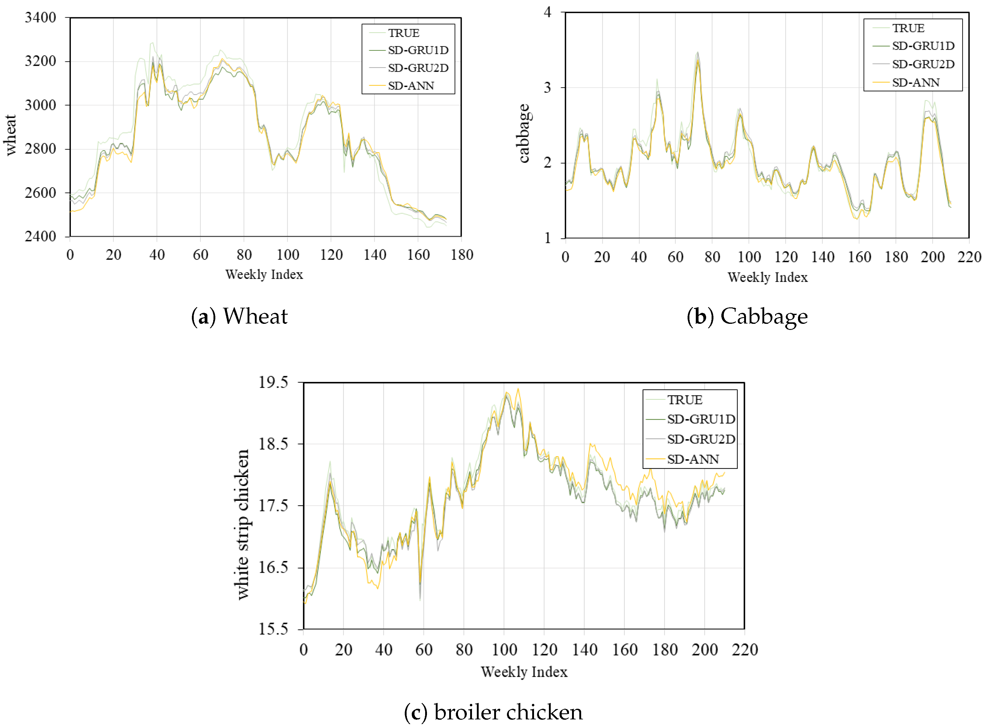
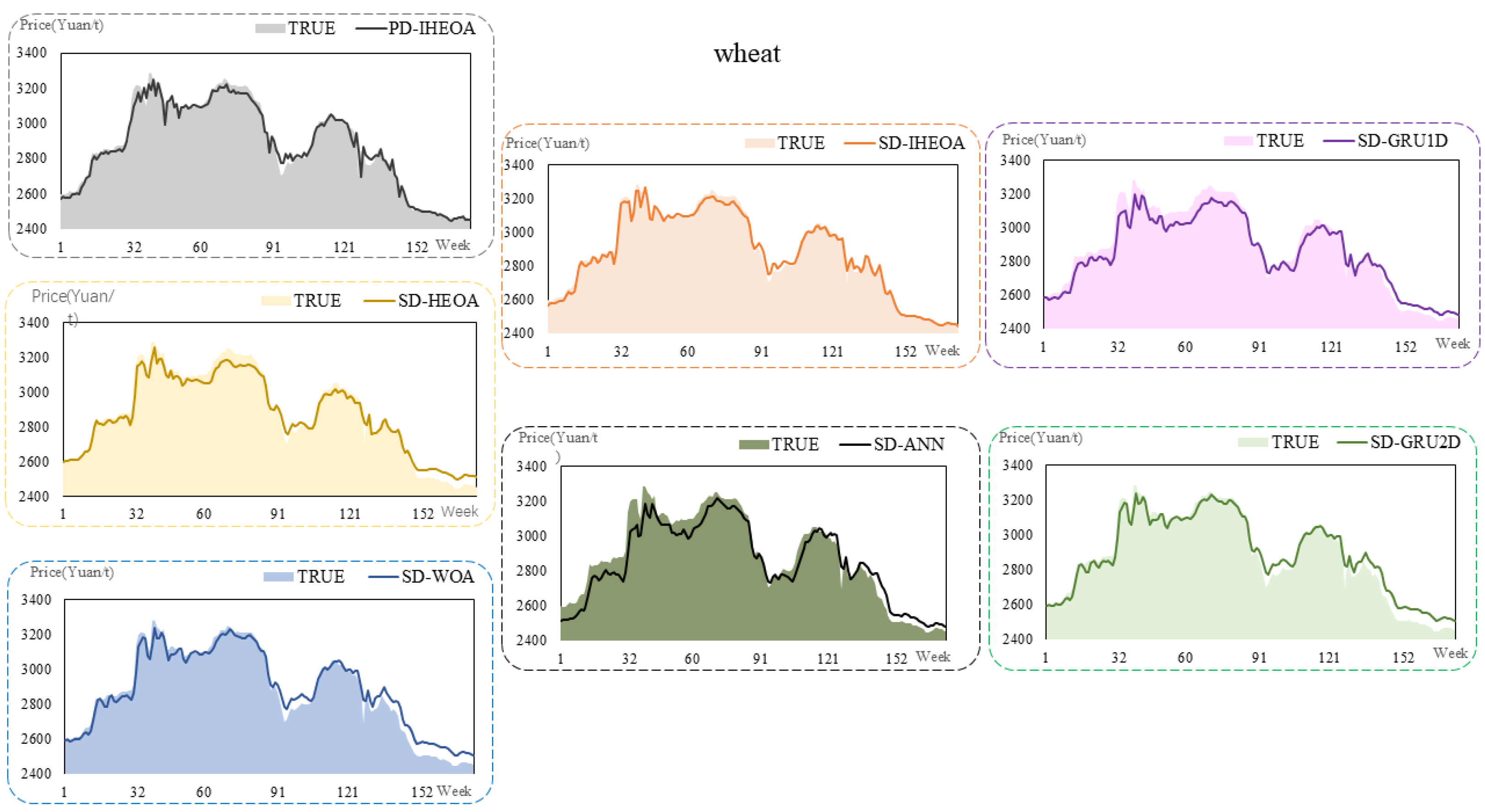
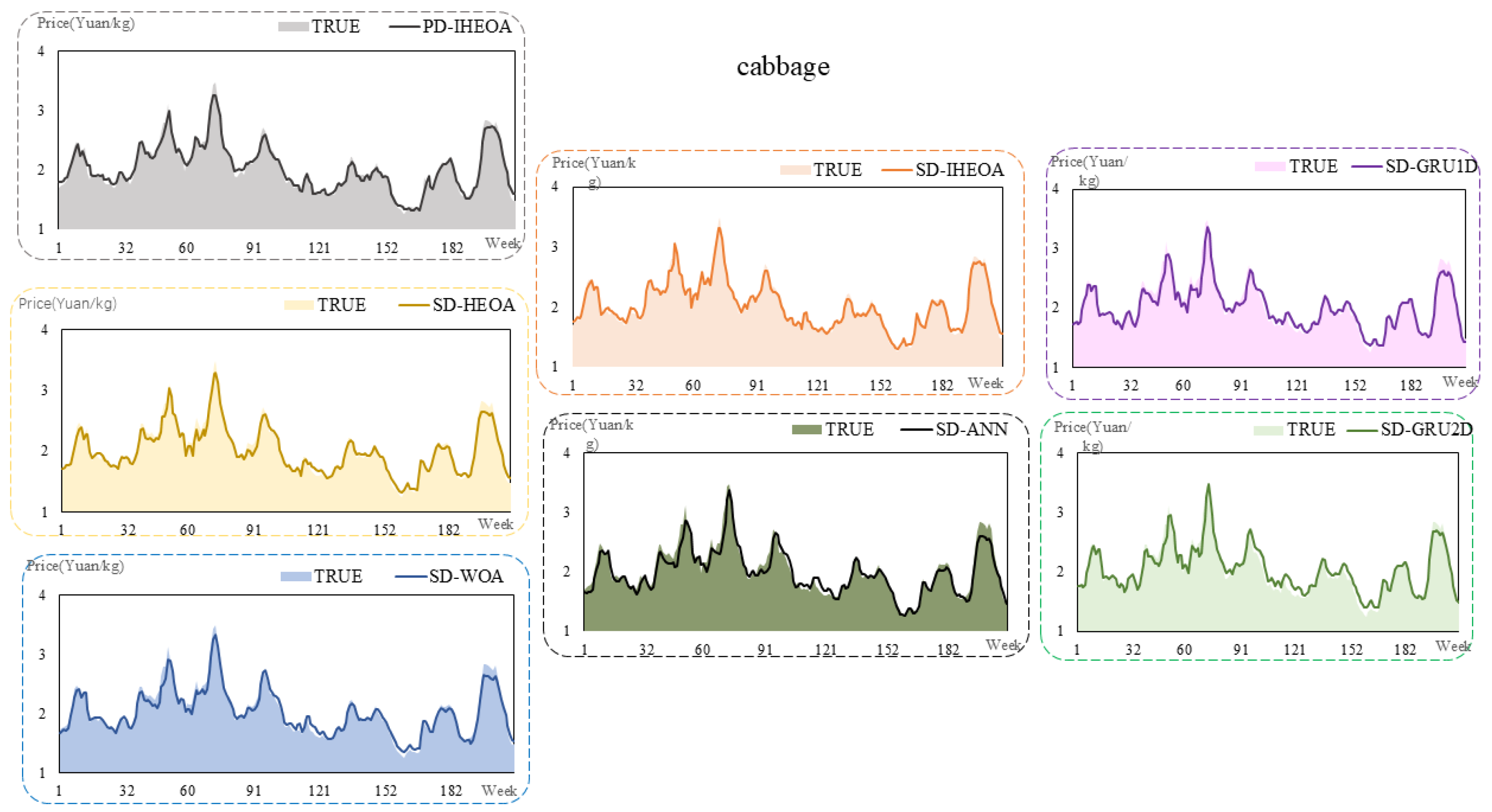
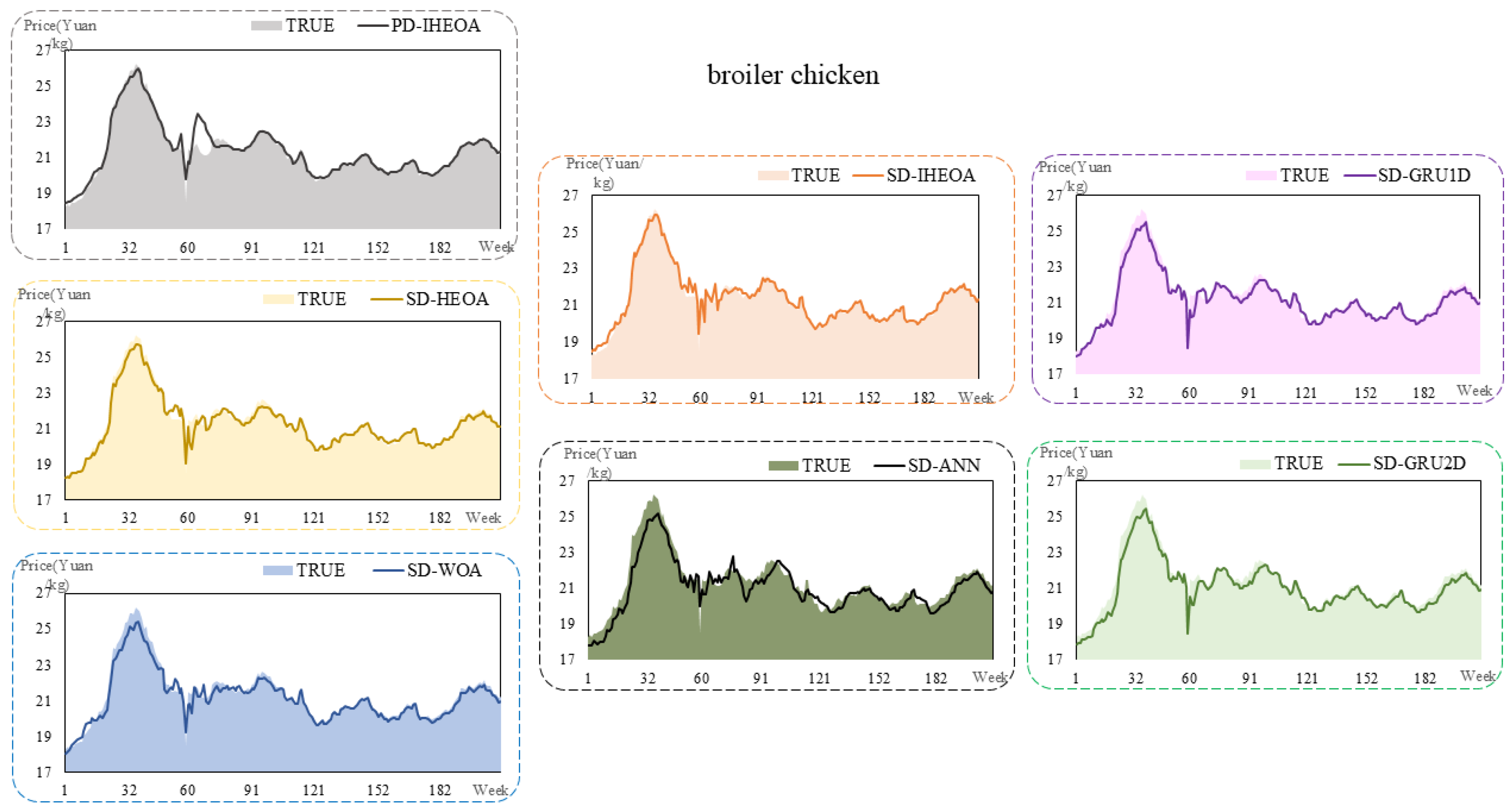
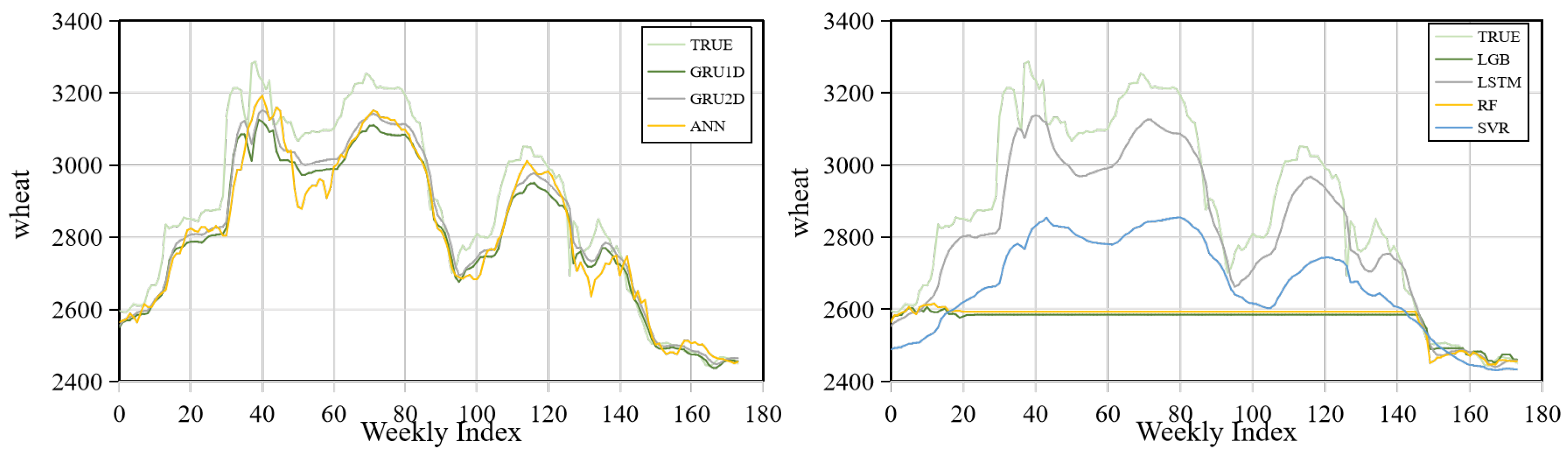
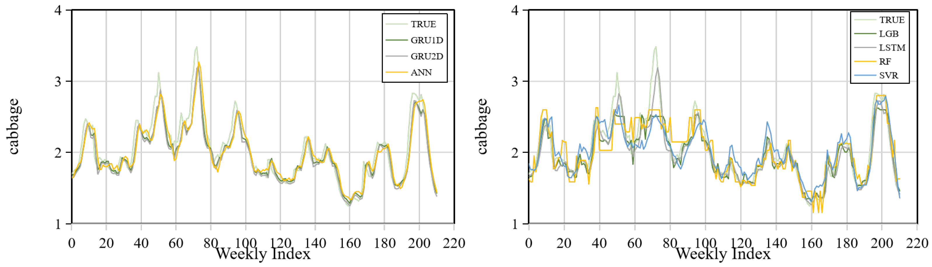
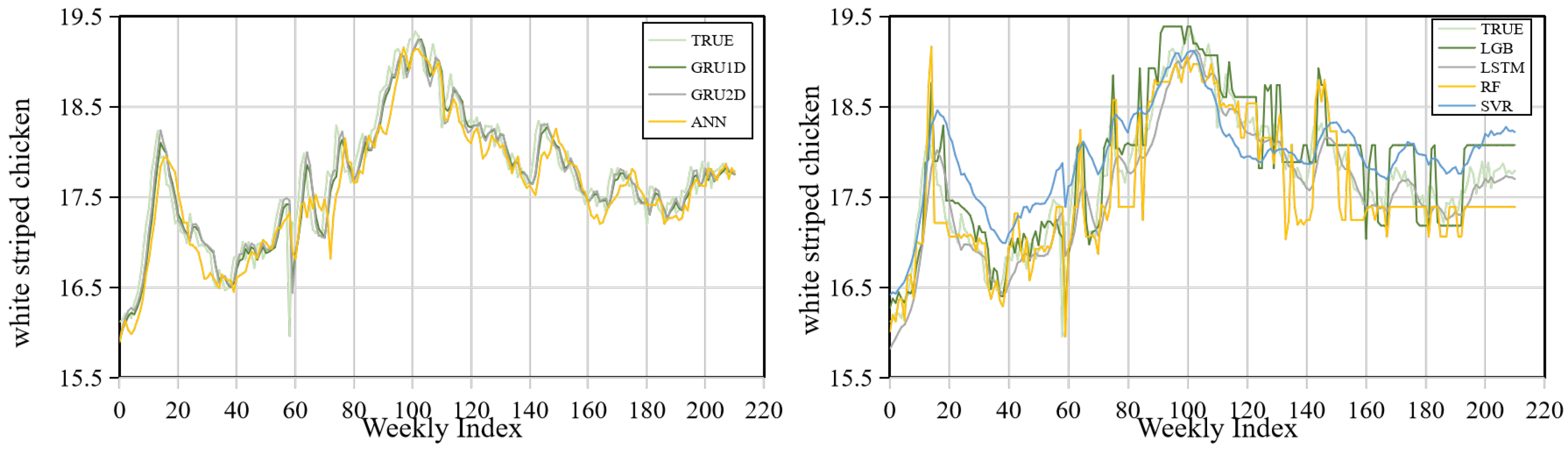
To validate the effectiveness of the model, the WOA (Whale Optimization Algorithm) algorithm and ANN (Artificial Neural Network) model are now introduced for verification. The fitting curves of prediction results and the true values in the test set are shown in
Figure 6,
Figure 7 and
Figure 8. The curves shown in orange, gray, yellow, blue, light green, pink, and dark green correspond to SD-IHEOA, PD-IHEOA, SD-HEOA, SD-WOA, SD-GRU2D, SD-GRU1D, and SD-ANN, respectively. Overall, the fitting curves indicate a high similarity between the predicted results and true values across all three categories of agricultural products, with consistent fluctuation patterns. From
Figure 7,
Figure 8 and
Figure 9, the SD-IHEOA model performs best in capturing the overall trend and periodic fluctuations of agricultural product prices, showing the highest agreement with true values. By comparison, the SD-ANN approach exhibits more pronounced prediction errors, particularly in periods characterized by abrupt price changes. The SD-HEOA and SD-IHEOA models deliver moderate results, successfully tracking the overall long-term tendency of price movements, yet showing limitations in accurately reflecting short-term fluctuations. In general, the SD-IHEOA optimized framework achieves the best forecasting performance among all considered models, highlighting its stronger fitting capability for agricultural price prediction tasks.
The study systematically evaluated the applicability of seven prediction models—SD-IHEOA, PD-IHEOA, SD-HEOA, SD-WOA, SD-ANN, SD-GRU1D, and SD-GRU2D—across five major agricultural product price series. The models’ performances underwent comprehensive assessment using statistical metrics including
, MAE, MAPE, and MSE. The evaluation results are presented in
Table 9,
Table 10,
Table 11,
Table 12,
Table 13,
Table 14,
Table 15,
Table 16,
Table 17,
Table 18,
Table 19 and
Table 20.
Table 9.
indicators for individual models of wheat prices.
Table 9.
indicators for individual models of wheat prices.
| | SD-IHEOA | PD-IHEOA | SD-HEOA | SD-WOA | SD-ANN | SD-GRU1D | SD-GRU2D |
|---|
| IMF0 | \ | \ | – | – | – | – | – |
| IMF0(SD) | 58.72% | – | 46.91% | 48.05% | 35.96% | 44.80% | 45.86% |
| IMF1 | 86.34% | 86.34% | 71.96% | 68.73% | 65.16% | 67.76% | 67.10% |
| IMF2 | 93.92% | 93.92% | 91.74% | 92.99% | 89.68% | 89.79% | 90.64% |
| IMF3 | 99.60% | 99.60% | 96.37% | 95.62% | 93.63% | 93.93% | 95.59% |
| IMF4 | 99.73% | 99.73% | 97.18% | 96.77% | 94.10% | 95.85% | 96.75% |
| IMF5 | 98.78% | 98.78% | 98.24% | 98.03% | 97.47% | 97.27% | 96.54% |
| Refactored results | 98.62% | 97.43% | 95.96% | 95.18% | 89.62% | 91.54% | 93.69% |
Table 10.
MAE indicators for individual models of wheat prices.
Table 10.
MAE indicators for individual models of wheat prices.
| | SD-IHEOA | PD-IHEOA | SD-HEOA | SD-WOA | SD-ANN | SD-GRU1D | SD-GRU2D |
|---|
| IMF0 | 19.5334 | 19.5334 | – | – | – | – | – |
| IMF0(SD) | 10.6028 | – | 9.5467 | 9.6087 | 10.2272 | 9.9980 | 9.9477 |
| IMF1 | 4.6316 | 4.6316 | 5.0182 | 8.8323 | 9.1573 | 8.3432 | 8.3060 |
| IMF2 | 12.6959 | 12.6959 | 14.8706 | 12.9002 | 20.1110 | 19.1955 | 19.1154 |
| IMF3 | 4.9518 | 4.9518 | 13.0014 | 15.2234 | 14.9750 | 17.1651 | 16.1645 |
| IMF4 | 9.8062 | 9.8062 | 27.4300 | 29.7472 | 39.3960 | 33.4206 | 31.1152 |
| IMF5 | 5.3782 | 5.3782 | 6.2790 | 6.9638 | 7.6677 | 8.3387 | 9.3368 |
| Refactored results | 21.7252 | 27.3391 | 36.2480 | 38.5634 | 58.5630 | 51.1372 | 46.4079 |
Table 11.
MAPE indicators for individual models of wheat prices.
Table 11.
MAPE indicators for individual models of wheat prices.
| | SD-IHEOA | PD-IHEOA | SD-HEOA | SD-WOA | SD-ANN | SD-GRU1D | SD-GRU2D |
|---|
| IMF0 | 3.4457 | 3.4457 | – | – | – | – | – |
| IMF0(SD) | 15.6058 | – | 5.0591 | 11.5135 | 25.4509 | 9.9646 | 20.3458 |
| IMF1 | 0.9337 | 0.9337 | 0.5807 | 1.9676 | 1.5215 | 4.0458 | 10.1391 |
| IMF2 | 0.3433 | 0.3433 | 0.5784 | 0.3514 | 1.4144 | 0.9870 | 1.7404 |
| IMF3 | 0.1411 | 0.1411 | 0.2119 | 0.7540 | 0.8738 | 0.9061 | 0.8386 |
| IMF4 | 0.2848 | 0.2848 | 0.3139 | 0.6219 | 0.7744 | 22.5905 | 0.5519 |
| IMF5 | 0.0019 | 0.0019 | 0.0022 | 0.0024 | 0.0027 | 0.0029 | 0.0033 |
| Refactored results | 0.0074 | 0.0094 | 0.0126 | 0.0137 | 0.0206 | 0.0177 | 0.0162 |
Table 12.
MSE indicators for individual models of wheat prices.
Table 12.
MSE indicators for individual models of wheat prices.
| | SD-IHEOA | PD-IHEOA | SD-HEOA | SD-WOA | SD-ANN | SD-GRU1D | SD-GRU2D |
|---|
| IMF0 | 1020.66 | 1020.66 | – | – | – | – | – |
| IMF0(SD) | 298.88 | – | 277.41 | 266.57 | 276.63 | 283.59 | 302.07 |
| IMF1 | 38.62 | 38.62 | 74.15 | 130.26 | 138.48 | 118.52 | 120.06 |
| IMF2 | 273.08 | 273.08 | 362.50 | 323.17 | 652.31 | 523.15 | 511.14 |
| IMF3 | 31.27 | 31.27 | 215.66 | 284.10 | 419.92 | 365.23 | 331.51 |
| IMF4 | 115.64 | 115.64 | 935.93 | 1062.81 | 1908.93 | 1344.39 | 1118.22 |
| IMF5 | 29.75 | 29.75 | 41.73 | 54.89 | 84.15 | 69.75 | 87.31 |
| Refactored results | 801.28 | 1487.41 | 1875.88 | 2318.59 | 5030.76 | 3786.58 | 3156.13 |
Numerical comparisons show that in the reconstruction results, the proposed SD-IHEOA model achieves the best performance across all four metrics, with an of 98.62%, MAE of 21.73, MAPE of 0.01, and MSE of 801.28, confirming the model’s effectiveness. For component-level predictions, the SD-IHEOA model performs exceptionally well on multiple components (IMF1 to IMF5). Its values for IMF1 to IMF5 reach 86.34%, 93.92%, 99.60%, 99.73%, 98.73%, and 98.78%, significantly outperforming SD-HEOA, SD-WOA, SD-ANN, SD-GRU1D, and SD-GRU2D models. Additionally, the SD-HEOA model shows good performance in predicting the high-frequency component IMF0(SD), with an of 46.91%. Although lower than SD-IHEOA, it achieves MAE of 9.55, MAPE of 5.06, and MSE of 277.41, all better than other models. While SD-WOA’s metrics fall below those of the IHEOA and HEOA combined models, it still surpasses models without metaheuristic optimization. Comparing IMF0 and IMF0(SD), IMF0(SD) shows better , MAE, and MSE, demonstrating the effectiveness of the secondary decomposition algorithm in predicting high-frequency components. For overall data reconstruction, the SD-IHEOA model also performs best, with an of 98.62%, MAE of 21.73, MAPE of 0.0074, and MSE of 801.28, all significantly lower than those of other models.
Table 13.
indicators for individual models of cabbage prices.
Table 13.
indicators for individual models of cabbage prices.
| | SD-IHEOA | PD-IHEOA | SD-HEOA | SD-WOA | SD-ANN | SD-GRU1D | SD-GRU2D |
|---|
| IMF0 | \ | \ | – | – | – | – | – |
| IMF0(SD) | 74.89% | – | 73.65% | 72.18% | 62.33% | 69.99% | 71.57% |
| IMF1 | 97.57% | 97.57% | 93.78% | 93.65% | 87.38% | 91.59% | 91.46% |
| IMF2 | 95.42% | 95.42% | 94.45% | 94.12% | 89.86% | 91.40% | 92.40% |
| IMF3 | 99.50% | 99.50% | 97.87% | 97.61% | 94.69% | 96.16% | 96.98% |
| IMF4 | 99.98% | 99.98% | 97.07% | 96.92% | 92.91% | 95.93% | 94.90% |
| IMF5 | 99.92% | 99.92% | 98.88% | 98.50% | 96.47% | 98.19% | 98.33% |
| IMF6 | 99.17% | 99.17% | 98.36% | 98.09% | 96.59% | 96.08% | 97.49% |
| Refactored results | 97.94% | 96.03% | 95.32% | 94.52% | 91.06% | 90.87% | 92.35% |
Table 14.
MAE indicators for individual models of cabbage prices.
Table 14.
MAE indicators for individual models of cabbage prices.
| | SD-IHEOA | PD-IHEOA | SD-HEOA | SD-WOA | SD-ANN | SD-GRU1D | SD-GRU2D |
|---|
| IMF0 | 0.0465 | 0.0465 | – | – | – | – | – |
| IMF0(SD) | 0.0239 | – | 0.0237 | 0.0223 | 0.0257 | 0.0238 | 0.0240 |
| IMF1 | 0.0218 | 0.0218 | 0.0336 | 0.0346 | 0.0516 | 0.0433 | 0.0483 |
| IMF2 | 0.0294 | 0.0294 | 0.0343 | 0.0348 | 0.0445 | 0.0397 | 0.0383 |
| IMF3 | 0.0110 | 0.0110 | 0.0210 | 0.0243 | 0.0292 | 0.0291 | 0.0278 |
| IMF4 | 0.0027 | 0.0027 | 0.0283 | 0.0324 | 0.0467 | 0.0369 | 0.0397 |
| IMF5 | 0.0007 | 0.0007 | 0.0022 | 0.0027 | 0.0040 | 0.0030 | 0.0025 |
| IMF6 | 0.0027 | 0.0027 | 0.0040 | 0.0040 | 0.0055 | 0.0062 | 0.0048 |
| Refactored results | 0.0440 | 0.0588 | 0.0620 | 0.0660 | 0.0848 | 0.0816 | 0.0841 |
Table 15.
MAPE indicators for individual models of cabbage prices.
Table 15.
MAPE indicators for individual models of cabbage prices.
| | SD-IHEOA | PD-IHEOA | SD-HEOA | SD-WOA | SD-ANN | SD-GRU1D | SD-GRU2D |
|---|
| IMF0 | 8.3498 | 8.3498 | – | – | – | – | – |
| IMF0(SD) | 1.9644 | – | 1.4644 | 3.0263 | 4.3006 | 4.5634 | 3.7591 |
| IMF1 | 0.7222 | 0.7222 | 1.0128 | 0.7105 | 1.1518 | 1.4980 | 3.0130 |
| IMF2 | 0.3850 | 0.3850 | 0.5601 | 0.9469 | 0.8718 | 1.4484 | 0.6897 |
| IMF3 | 0.1507 | 0.1507 | 0.3469 | 2.5336 | 0.6239 | 0.9264 | 0.6242 |
| IMF4 | 0.0126 | 0.0126 | 0.1307 | 0.2698 | 0.3913 | 1.0185 | 0.3105 |
| IMF5 | 0.0834 | 0.0834 | 0.1547 | 0.1558 | 0.5927 | 0.3421 | 0.0924 |
| IMF6 | 0.0013 | 0.0013 | 0.0019 | 0.0019 | 0.0026 | 0.0030 | 0.0023 |
| Refactored results | 0.0216 | 0.0288 | 0.0300 | 0.0323 | 0.0409 | 0.0395 | 0.0412 |
Table 16.
MSE indicators for individual models of cabbage prices.
Table 16.
MSE indicators for individual models of cabbage prices.
| | SD-IHEOA | PD-IHEOA | SD-HEOA | SD-WOA | SD-ANN | SD-GRU1D | SD-GRU2D |
|---|
| IMF0 | 0.0037 | 0.0037 | – | – | – | – | – |
| IMF0(SD) | 0.0009 | – | 0.0009 | 0.0008 | 0.0010 | 0.0009 | 0.0009 |
| IMF1 | 0.0009 | 0.0009 | 0.0020 | 0.0024 | 0.0044 | 0.0036 | 0.0036 |
| IMF2 | 0.0013 | 0.0013 | 0.0021 | 0.0020 | 0.0033 | 0.0029 | 0.0026 |
| IMF3 | 0.0002 | 0.0002 | 0.0006 | 0.0007 | 0.0014 | 0.0011 | 0.0010 |
| IMF4 | 0.00001 | 0.00001 | 0.0013 | 0.0014 | 0.0028 | 0.0017 | 0.0021 |
| IMF5 | 0.000001 | 0.000001 | 0.00001 | 0.00001 | 0.00002 | 0.00001 | 0.00001 |
| IMF6 | 0.00001 | 0.00001 | 0.00002 | 0.00002 | 0.00004 | 0.00004 | 0.00003 |
| Refactored results | 0.0031 | 0.0060 | 0.0066 | 0.0075 | 0.0127 | 0.0122 | 0.0109 |
The experimental results for Chinese cabbage show that the SD-IHEOA model achieves the highest values in most IMF components, especially reaching 99.98% and 99.92% in IMF4 and IMF5 respectively, significantly outperforming other models. In terms of MAE, the SD-IHEOA model performs best across IMF1 to IMF6, with values of 0.0218, 0.0294, 0.0110, 0.0027, 0.0007, and 0.0027, all markedly lower than those of competing models. MAPE and MSE metrics further confirm the superiority of the SD-IHEOA model, showing substantially lower errors than others. Comparing IMF0 and IMF0(SD), IMF0(SD) outperforms in all four metrics, indicating the effectiveness of the secondary decomposition algorithm in predicting high-frequency components. The four evaluation metrics for reconstruction results also demonstrate that the SD-IHEOA model delivers the highest prediction accuracy and stability, with values of 97.94%, 0.0440, 0.0216, and 0.0031, all surpassing other models. These findings highlight the advantage of the SD-IHEOA model in capturing the trends and periodic variations of mid- to low-frequency components when processing Chinese cabbage data.
Table 17.
indicators for individual models of broiler chicken prices.
Table 17.
indicators for individual models of broiler chicken prices.
| | SD-IHEOA | PD-IHEOA | SD-HEOA | SD-WOA | SD-ANN | SD-GRU1D | SD-GRU2D |
|---|
| IMF0 | \ | \ | – | – | – | – | – |
| IMF0(SD) | 58.43% | – | 55.18% | 55.88% | 39.47% | 48.43% | 51.38% |
| IMF1 | 97.24% | 97.24% | 96.63% | 96.32% | 90.96% | 94.58% | 95.17% |
| IMF2 | 99.97% | 99.97% | 98.23% | 97.97% | 93.90% | 97.60% | 97.01% |
| IMF3 | 99.99% | 99.99% | 98.73% | 98.57% | 94.61% | 98.14% | 97.72% |
| IMF4 | 99.96% | 99.96% | 99.92% | 99.93% | 98.87% | 99.89% | 99.08% |
| IMF5 | 93.59% | 93.59% | 90.96% | 89.71% | 72.78% | 86.78% | 88.70% |
| Refactored results | 98.42% | 93.92% | 98.21% | 97.76% | 93.56% | 95.84% | 96.06% |
Table 18.
MAE indicators for individual models of broiler chicken prices.
Table 18.
MAE indicators for individual models of broiler chicken prices.
| | SD-IHEOA | PD-IHEOA | SD-HEOA | SD-WOA | SD-ANN | SD-GRU1D | SD-GRU2D |
|---|
| IMF0 | 0.0844 | 0.0844 | – | – | – | – | – |
| IMF0(SD) | 0.0398 | – | 0.0388 | 0.0394 | 0.0340 | 0.0410 | 0.0347 |
| IMF1 | 0.0196 | 0.0196 | 0.0211 | 0.0220 | 0.0348 | 0.0256 | 0.0242 |
| IMF2 | 0.0025 | 0.0025 | 0.0179 | 0.0206 | 0.0380 | 0.0216 | 0.0240 |
| IMF3 | 0.0026 | 0.0026 | 0.0278 | 0.0318 | 0.0644 | 0.0346 | 0.0402 |
| IMF4 | 0.0109 | 0.0109 | 0.0138 | 0.0108 | 0.0498 | 0.0119 | 0.0456 |
| IMF5 | 0.0363 | 0.0363 | 0.0523 | 0.0420 | 0.1047 | 0.0637 | 0.0578 |
| Refactored results | 0.0636 | 0.1146 | 0.0706 | 0.0777 | 0.1620 | 0.1151 | 0.1039 |
Table 19.
MAPE indicators for individual models of broiler chicken prices.
Table 19.
MAPE indicators for individual models of broiler chicken prices.
| | SD-IHEOA | PD-IHEOA | SD-HEOA | SD-WOA | SD-ANN | SD-GRU1D | SD-GRU2D |
|---|
| IMF0 | 5.1324 | 5.1324 | – | – | – | – | – |
| IMF0(SD) | 1.7937 | – | 4.5604 | 4.6696 | 0.0748 | 2.8745 | 0.0758 |
| IMF1 | 0.7616 | 0.7616 | 2.0537 | 0.8460 | 0.7438 | 1.6236 | 1.7099 |
| IMF2 | 0.0810 | 0.0810 | 1.2755 | 0.6173 | 1.9414 | 0.3112 | 0.4157 |
| IMF3 | 0.3752 | 0.3752 | 0.1411 | 0.5605 | 1.0493 | 0.5411 | 0.5735 |
| IMF4 | 0.2136 | 0.2136 | 0.2812 | 0.3532 | 0.5206 | 0.0636 | 0.3980 |
| IMF5 | 0.0020 | 0.0020 | 0.0030 | 0.0024 | 0.0059 | 0.0036 | 0.0032 |
| Refactored results | 0.0036 | 0.0065 | 0.0040 | 0.0044 | 0.0092 | 0.0066 | 0.0059 |
Table 20.
MSE indicators for individual models of broiler chicken prices.
Table 20.
MSE indicators for individual models of broiler chicken prices.
| | SD-IHEOA | PD-IHEOA | SD-HEOA | SD-WOA | SD-ANN | SD-GRU1D | SD-GRU2D |
|---|
| IMF0 | 0.0229 | 0.0229 | – | – | – | – | – |
| IMF0(SD) | 0.0035 | – | 0.0035 | 0.0034 | 0.0028 | 0.0039 | 0.0026 |
| IMF1 | 0.0008 | 0.0008 | 0.0008 | 0.0010 | 0.0022 | 0.0013 | 0.0012 |
| IMF2 | 0.000009 | 0.000009 | 0.0006 | 0.0007 | 0.0023 | 0.0008 | 0.0010 |
| IMF3 | 0.00001 | 0.00001 | 0.0014 | 0.0018 | 0.0062 | 0.0022 | 0.0029 |
| IMF4 | 0.0001 | 0.0001 | 0.0003 | 0.0003 | 0.0040 | 0.0004 | 0.0032 |
| IMF5 | 0.0019 | 0.0019 | 0.0029 | 0.0024 | 0.0131 | 0.0042 | 0.0034 |
| Refactored results | 0.0074 | 0.0280 | 0.0082 | 0.0101 | 0.0370 | 0.0198 | 0.0183 |
In the performance evaluation of the broiler chicken experiment, the model’s fitting results across different IMFs underwent quantitative analysis. For the metric, the SD-IHEOA model excelled in IMF2, IMF3, and IMF4, achieving values of 99.97%, 99.99%, and 99.96%, respectively, clearly outperforming other models. The SD-HEOA model’s value on IMF0(SD) reached 0.5518, slightly lower than SD-IHEOA’s 0.5843. Regarding MAE, the SD-IHEOA model performed best on IMF1, IMF3, IMF4, and IMF5, with values of 0.0196, 0.0026, 0.0109, and 0.0363, significantly lower than competing models. The MAPE metric further confirmed SD-IHEOA’s superiority on IMF2, IMF3, and IMF5, with values of 0.0810, 0.3752, and 0.0020, respectively, all below other models. On MSE, SD-IHEOA showed the best performance from IMF1 to IMF5, with values markedly lower than the rest.Comparing IMF0 and IMF0(SD), all four metrics favored IMF0(SD), demonstrating the effectiveness of the secondary decomposition algorithm in predicting high-frequency components. The reconstruction metrics also indicate that SD-IHEOA delivers the highest prediction accuracy and stability, with R2, MAE, MAPE, and MSE values of 98.42%, 0.0636, 0.0036, and 0.0074, respectively, outperforming other models. These results confirm that SD-IHEOA holds a significant advantage in processing broiler chicken data, particularly in capturing trends and periodic variations of mid- to low-frequency components.
To verify whether the improvement of the proposed SD-IHEOA model is statistically significant, the Diebold–Mariano (DM) test was performed. The results in
Table 21 show that the differences in forecasting accuracy between the proposed and benchmark models are statistically significant (
p < 0.05), confirming the robustness of the proposed method.