Article

Urban Heat Island: Assessing the Influence of Urban Morphology on Air and Surface Temperatures

Department of Civil, Chemical, Environmental and Materials Engineering (DICAM), Università di Bologna, Viale Risorgimento 2, 40136 Bologna, Italy
*
Author to whom correspondence should be addressed.
Sustainability 2026, 18(3), 1695; https://doi.org/10.3390/su18031695
Submission received: 11 December 2025 / Revised: 21 January 2026 / Accepted: 30 January 2026 / Published: 6 February 2026

Abstract

This study investigates the interplay between urban morphology, vegetation, and thermal environments by integrating mobile air temperature (AT) measurements with satellite-derived land surface temperature (LST). The case study is the city of Bologna (Italy). Correlation analysis revealed strong multicollinearity among morphological indicators, with building density and floor area ratio nearly collinear, while vegetation cover (PV) remained the most independent predictor. A composite urban density indicator (CUDI), derived through principal component analysis, was introduced to address redundancy among morphological metrics. Ordinary least squares regressions demonstrated significant associations, with PV exerting a pronounced cooling effect and CUDI amplifying both AT and LST. Model diagnostics confirmed statistical robustness, though residual spatial autocorrelation necessitated spatial regression approaches. Spatial lag models (SLMs) substantially improved explanatory power, highlighting spatial spillovers and neighborhood effects as central to understanding urban heat dynamics. Comparative analysis with spatial error models reinforced the dominance of SLM in capturing localized dependencies. Despite limitations in spatial coverage, temporal scope, and indicator transferability, findings emphasize the critical roles of vegetation and urban compactness in shaping thermal environments. This work underscores the necessity of integrating greening strategies with urban form management for effective heat mitigation and provides a methodological framework for analyzing urban heat islands through multi-source thermal and morphological data.

Graphical Abstract

1. Introduction

The urban heat island (UHI) effect describes the phenomenon of increased air and surface temperatures in urban areas compared to surrounding rural areas [1,2]. The UHI effect is a significant concern because it can lead to various issues, including increased energy consumption for cooling, reduced air and water quality, and negative effects on human health and biodiversity [2,3,4]. One common method of calculating UHI intensity is determining the temperature difference between urban and rural areas. However, this process is complex and requires careful consideration of factors like terrain, land cover [4]. Accordingly, selecting proper data and indicators to quantify UHI are crucial for decision-makers in developing sustainable policies. Researchers commonly use both air temperature (AT) and land surface temperature (LST) data to investigate UHI effect [2,5]. AT is typically measured at ground-based meteorological stations, while LST is acquired through remote sensing techniques using satellite or airborne sensors [2,6,7]. While both AT and LST can quantify UHI intensity, they represent different aspects of the urban thermal environment [2,5]. Studies have shown that LST-based is generally stronger than AT-based UHI intensity, highlighting the differences in the data sources [2]. Understanding the relationship between AT and LST is essential for comprehensively assessing the UHI effect and developing effective mitigation strategies [2,5,6]. For instance, research has shown that evapotranspiration from vegetation plays a significant role in reducing both surface and canopy UHI intensity [4]. Therefore, increasing urban green spaces, particularly through strategic urban planning and design, can help alleviate the UHI effect by promoting evaporative cooling [4,8,9]. Other mitigation methods include using cool or reflective materials for roofs and pavements to reduce heat absorption, optimizing building design and orientation to enhance natural ventilation, and reducing anthropogenic heat emissions [8,10].
The city of Bologna, Italy, has been the subject of multiple studies examining the UHI effect and potential mitigation strategies. Bologna’s diverse urban landscape, with a mix of historic and modern structures, makes it a valuable case study for understanding the complex interplay of urban morphology and UHI intensity [11,12,13,14]. Research conducted by the authors in Bologna has demonstrated the effectiveness of combining mobile and static temperature measurements for comprehensive thermal analysis [13] and has highlighted the significant impact of building density on surface temperature variations within the city [14]. These studies can provide valuable insights for urban planners and policymakers, enabling the development of targeted measures to enhance urban resilience and mitigate the negative consequences of rising temperatures and climate change.
A city’s morphological characteristics, such as building density, height, and the presence of vegetation, play a crucial role in the UHI effect [1,14]. Denser urban areas with limited vegetation tend to experience more intense UHIs due to reduced wind flow and increased heat absorption by buildings and paved surfaces [9,10,15]. On the other hand, accurate UHI characterization and quantification require a thorough understanding of these morphological influences and necessitate reliable temperature data [2]. Various Urban Morphological Indices (UMIs) are defined and studied in relation to UHI intensity studies, including building density [9,14,15,16], building height [9,15,17], Sky View Factor (SVF) [9,15,17], green cover ratio [4,9,15], impervious plan area ratio [4,18], albedo [18], street network integration index [9], orientation variance of building [17], and mean aspect ratio [19]. The determination of which UMI is the most important often depends on the specific scale of the study (i.e., local or city-wide), the climate, the season, and whether AT or LST is being measured [2,18]. However, comprehensive quantitative studies highlight certain parameters as consistently dominant factors influencing the urban thermal environment. Among these, the Normalized Difference Vegetation Index (NDVI) is widely employed as a proxy for vegetation abundance and vigor, serving as a critical indicator of cooling capacity through evapotranspiration [9,15,17,19]. The percentage of built-up area or impervious surface area captures the extent of sealed surfaces that intensify heat storage and restrict natural cooling [18,20]. Similarly, Building Density (BD) and Floor Area Ratio (FAR) represent morphological compactness and the intensity of land use, both of which strongly correlate with heat accumulation and reduced ventilation [18,20]. Finally, Mean Building Height (MBH) reflects the vertical dimension of urban form, influencing shading, wind circulation, and radiative exchanges [15,18]. Collectively, these parameters constitute the core set of indicators most frequently identified as shaping the urban thermal environment in quantitative UHI studies. Researchers use these indicators to understand how the physical layout and structure of urban areas influence UHI intensity. Despite this extensive body of research, few studies have systematically compared how these dominant UMIs simultaneously influence canopy-level air and surface temperature within the same urban context, while explicitly accounting for spatial dependence and multicollinearity among indicators. Moreover, empirical evidence linking mobile AT measurements with high-resolution satellite-derived LST remains limited, particularly for medium-sized historic European cities such as Bologna, where complex urban morphology may alter thermal responses.
To enable a more comprehensive comparative analysis of the canopy and surface UHI, this study utilizes LST data retrieved from ECOSTRESS imagery along with AT measurements acquired and corrected through a mobile survey. The primary objectives are to assess the impact of various UMIs on both AT and LST, and to investigate the correlation between AT and LST. Thus, the objectives of this research are to (i) evaluate the differential impacts of key urban morphology indicators and vegetation on AT and LST, accounting for multicollinearity; (ii) systematically characterize and model spatial autocorrelation and neighborhood spillover processes in the urban thermal system; and (iii) develop a framework for coordinated mitigation strategies integrating greening interventions and urban form regulation in Bologna. The findings are expected to enhance understanding of UHI dynamics and assist future researchers in selecting suitable data sources and indicators for studying urban thermal variations and to develop effective mitigation strategies, such as increasing green spaces, using cool materials, and optimizing building design.

2. Materials and Methods

2.1. Data Collection and Sources

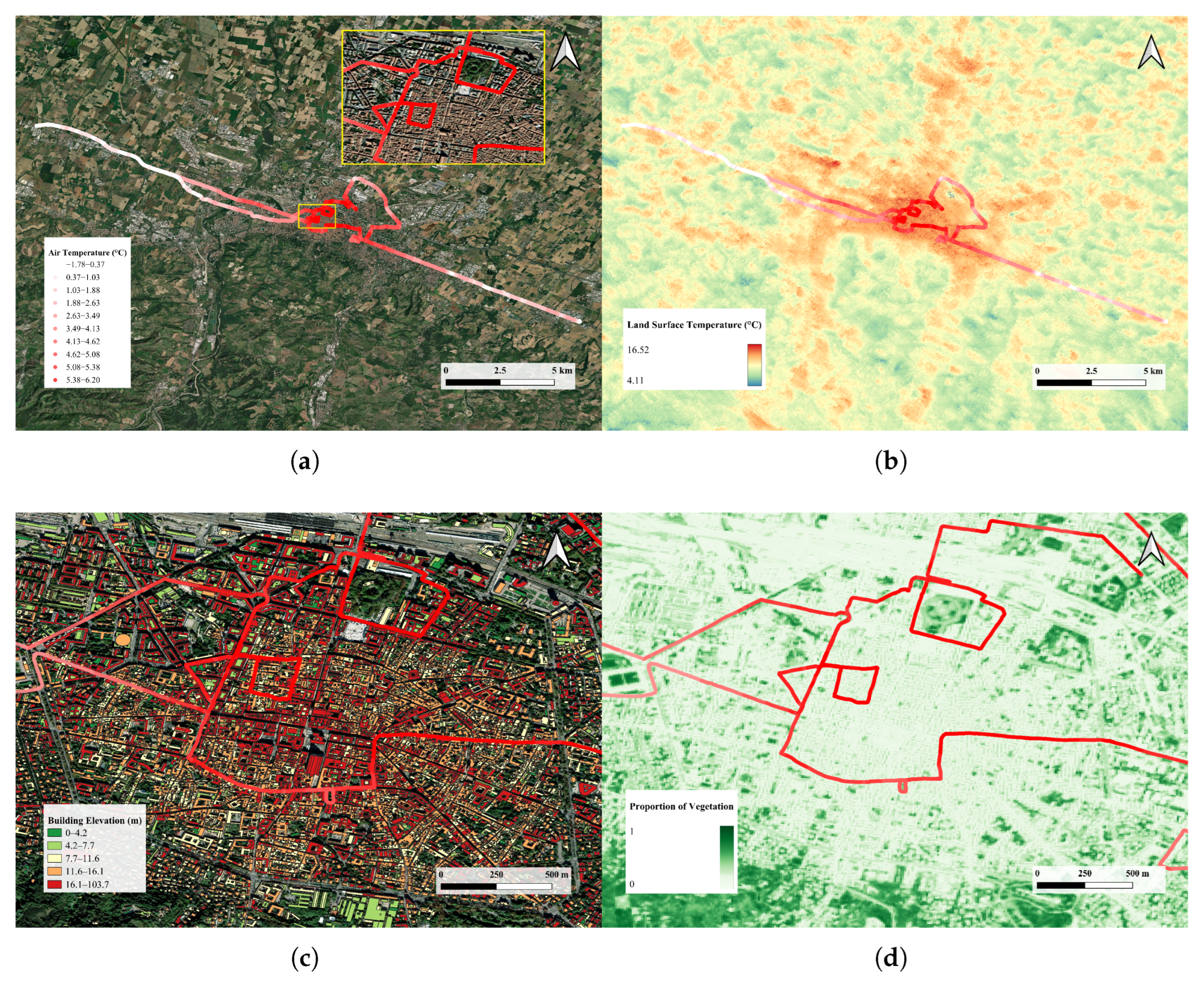
Nocturnal AT data used in this study were derived from our previously published mobile transect measurements [13,14]. Figure 1 presents a schematic diagram of the system used for AT recording. Measurements were taken along a transect path (Figure 2a), and the recorder temperature data were corrected using readings from fixed weather stations and thermometers positioned along the transect. For a detailed description of this correction readers are referred to [13]. This adjustment was necessary to enhance the temporal accuracy and spatial relevance of the collected temperature data. By utilizing these corrected AT data, the present study ensures a robust basis for investigating the relationship between UMIs and both air and land surface temperatures.
LST data for Bologna were sourced from the NASA Earth Data platform (A ρ ρ EEARS) [21]. The selection of LST data was constrained by both observational availability and specific criteria to ensure temporal correspondence with the nocturnal AT measurements and minimal cloud contamination (less than 10%). Initially, multiple satellite sources were assessed for the date of the AT campaign, including Sentinel-3A, Landsat 8, and NASA A ρ ρ EEARS. Only one Sentinel-3A image was present for the transect date, recorded on 21 March 2021 at 21:54 local time with spatial resolution 1 km [22]. The spatial resolution is not enough for the analysis. Furthermore, it exhibited 54.40% cloud-contaminated pixels which made it unsuitable for analysis. To overcome these limitations, the search focused on the most temporally proximate, LST acquisitions. Two candidates emerged, the Landsat 8 image on 18 March 2021 at 10:58 local time with a spatial resolution of 25 m2 [23] and a NASA ECOSTRESS image from 24 March 2021, at 16:58:54 UTC (17:58:54 local time) and with a spatial resolution of 70 m (Figure 2b) [21]. The Landsat 8 scene presented over-land cloud coverage of 41.55%, also preventing reliable LST retrieval. Consequently, the ECOSTRESS Level-2 product was selected as the optimal source of LST, representing the best compromise between temporal proximity, spatial resolution, and atmospheric conditions. The ECOSTRESS mission, launched by NASA on the International Space Station in 2018, aims to measure LST and evapotranspiration using high-resolution thermal infrared data to better understand plant water use and stress across Earth’s ecosystems [24,25]. The ECOSTRESS image was cloud-free, with 91.78% of pixels validated through quality control, capturing urban heterogeneity while maintaining adequate regional coverage. The LST data, originally in Kelvin, were converted to degrees Celsius to facilitate analysis and interpretation.
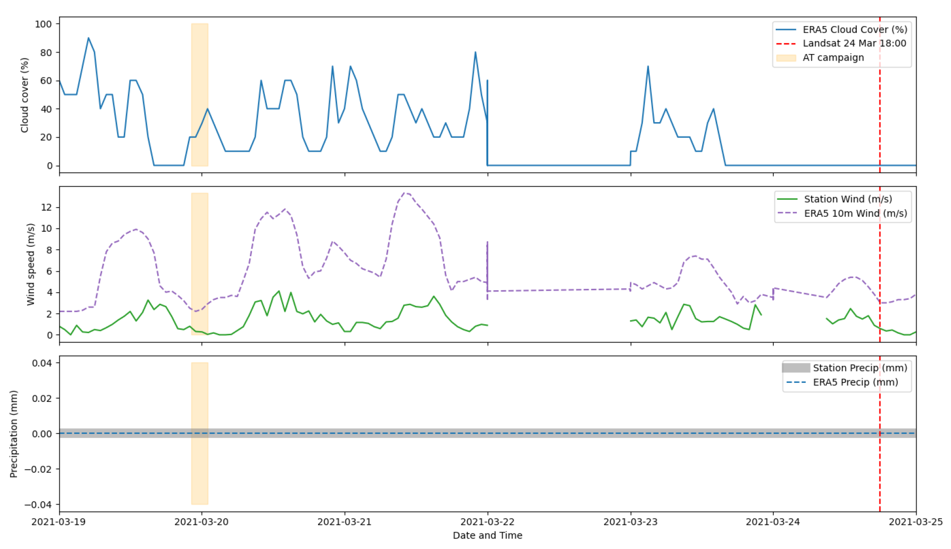
Given the difference in acquisition dates between the AT campaign and the ECOSTRESS overpass, a temporal harmonization assessment was conducted. ERA5 reanalysis (0.25° resolution) [26] and a local weather station (44.49° N, 11.33° E, 72 m a.s.l.) [27] provided hourly observations for 19–25 March, including AT, wind gusts, skin temperature, precipitation, and cloud cover. Diagnostic windows were defined for the AT campaign (19 March 22:16–20 March 00:57) and the ECOSTRESS acquisition (24 March 17:59 ± 24 h). Both datasets indicated stable meteorological conditions of no precipitation, negligible cloud cover (0% at the ECOSTRESS overpass), and calm wind regimes (differences less than 1 m/s) (Figure 3). Temperature values reflected expected diurnal variation rather than differing atmospheric regimes, AT of 3.1 °C (with ERA5 skin temperature of −1.18 ℃) versus ECOSTRESS LST of 12.32 °C and corresponding ERA5 skin temperatures of 10.15 °C. These results demonstrate that, despite being acquired on different days and times, the two datasets are meteorologically equivalent, ensuring that AT-LST comparisons reflect genuine surface-atmosphere thermal dynamics rather than confounding weather variability. This approach aligns with prior studies emphasizing the importance of meteorological equivalence when comparing ground-based and remotely sensed temperature data [28], ensuring that observed correlations reflect genuine surface-atmosphere thermal dynamics rather than external atmospheric variability.
Information on buildings in Bologna was obtained from the Municipality of Bologna’s open data platform [29] (Figure 2c). This dataset provided details on the building’s height, area, and volume, which were essential for calculating UMIs. Building on the indicators previously applied in [14], this study introduces a new composite metric, the Composite Urban Density Index (CUDI), to address redundancy and multicollinearity among commonly used built-form indicators by integrating BD, FAR, and MBH into a single, physically meaningful measure of urban compactness and volumetric intensity. A thorough quality control process was conducted on this dataset before analysis. Temporary structures, such as kiosks and shelters, were excluded; buildings under construction were checked using historical imagery from Google Earth Pro to verify their existence in March 2021; and for buildings missing height data, LiDAR DSMs [30] and Google Earth Pro 3D visualization tool was employed to estimate and fill in the missing values.
The NDVI data were derived from Sentinel-2 satellite imagery, acquired on 24 March 2021, with a spatial resolution of 10 m (Figure 2d) [22]. From the NDVI values, the Proportion of Vegetation (PV) was calculated using Equation (1), which serves as an indicator of vegetation coverage within the study area. Unlike our previous studies, here PV is systematically integrated alongside CUDI to examine its combined influence with urban form on both corrected AT and LST patterns.

2.2. Block Definition and Calculation of Urban Morphology Indicators (UMIs)

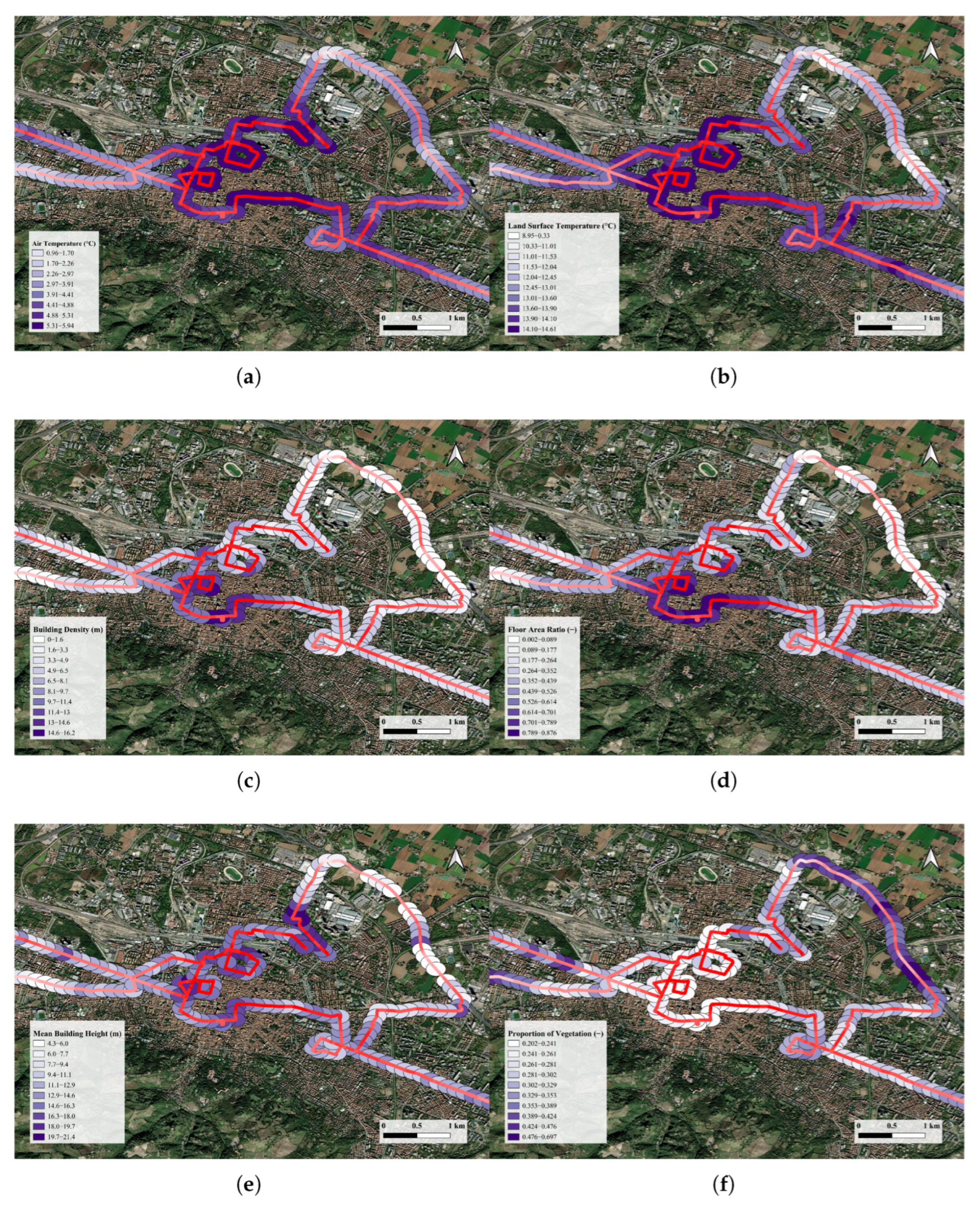
To facilitate analysis along the mobile transect, spatially consistent blocks were defined based on the distance between AT measurement points. Mobile data points separated by 150 m were selected, and each point was buffered by 150 m. The buffer size was guided by the coarsest spatial resolution among the datasets, specifically, the 70-m resolution of the LST data. Despite a nominal spatial resolution of 70 m, which could theoretically support a finer analysis grid, a larger buffer was intentionally adopted as a spatial aggregation and smoothing strategy to better represent the thermal environment sampled by mobile measurements. Specifically, this buffer size serves three purposes: (i) it reduces noise associated with instantaneous mobile AT readings that are influenced by short-term atmospheric fluctuations, traffic effects, and positional uncertainty [31]; (ii) it defines an analysis unit that is more representative of a neighborhood-scale thermal environment rather than point-scale micro-variability; and (iii) it ensures that a sufficient number of LST pixels and urban morphological features (such as buildings and land cover elements) are included within each unit to support stable indicator calculation and averaging. Using a buffer larger than the native LST pixel size also mitigates potential geolocation mismatch between datasets and improves the robustness of AT-LST comparisons. This buffer-based aggregation approach is consistent with established practices in mobile and urban climate studies, where spatial averaging is commonly applied to enhance representativeness and reduce measurement noise when linking mobile temperature observations with remotely sensed and morphological indicators [31,32,33,34]. Moreover, to evaluate the potential oversmoothing effect of the selected 150-m buffer, a sensitivity analysis was conducted by comparing results derived from 50-m and 150-m spatial units. Mean AT and LST were highly consistent across scales (mean AT: 3.04 °C at 50-m vs. 2.95 °C at 150-m; mean LST: 12.50 °C vs. 12.39 °C). Spatial variability decreased only marginally with increasing buffer size, with spatial standard deviation reductions of 2.7% for AT and 6.3% for LST, indicating limited smoothing of neighborhood-scale thermal heterogeneity. The AT-LST relationship remained stable across scales (r = 0.89 at both 50-m and 150-m), and distributional characteristics were preserved, as evidenced by similar quantiles. These results demonstrate that the selected 150-m buffer provides a robust balance between noise reduction and preservation of meaningful spatial thermal variability. In total, 352 buffers were created, which served as the analytical blocks where mean AT, LST, and UMIs were calculated (Figure 4).
Based on the data availability and relevance to urban thermal processes, four UMIs were selected for the analysis and calculated in a GIS environment. The selection of PV, MBH, BD, and FAR as urban morphological indicators is based on their capacity to capture the most fundamental and interpretable dimensions of urban form that drive UHI dynamics. These indicators represent the most fundamental, accessible, and widely validated variables for characterizing urban form and ecology, capturing vegetation cover, horizontal density, vertical structure, and overall volumetric intensity [15,35,36]. Together, they describe the core dimensions of urban morphology (density, height, volume, and vegetation) that are known to regulate surface energy balance, airflow, shading, and evapotranspiration, and thus strongly influence urban heat island dynamics [8,35]. Compared with more specialized indicators such as SVF or surface albedo, which often require complex modeling or high-resolution data and can be highly context-specific [9,11,37,38], these variables can be reliably derived from widely available datasets, are computationally straightforward, and have been extensively applied and validated in urban climate and UHI studies [15,35], making them suitable for comparative and scalable analysis across urban contexts.
Equation (1) shows P V indicator derived from N D V I data, where m i n and m a x show the minimum and maximum values of N D V I , and P V will have a value between 0 and 1. Equation (2) represents M B H which indicates the average height of buildings within each defined block. Here, H i denotes the height of the i-th building, and n is the total number of buildings that intersect with the block. Equation (3) represents B D defined as the total building volume ( V i ) within a block per unit area of the block (A). F A R is the fourth indicator providing an indication of building coverage intensity and A i is the building floor area of the i-th building (Equation (4)).
P V = N D V I N D V I min N D V I max N D V I min 2
M B H = i = 1 n H i n
B D = i = 1 n V i A
F A R = i = 1 n A i A

2.3. Statistical Approach

With the full dataset assembled, the next step involved removing outliers and normalizing the data. Outliers were determined by defining a lower and upper bound based on the data mean, standard deviation, and a sensitivity k value (Equations (5) and (6)).
Lower   Band = μ ( k × σ )
Upper   Band = μ + ( k × σ )
where μ is the mean, σ the standard deviation, and k the sensitivity coefficient (it is selected to be k = 3 ) [39]. Specifically, for each variable (MBH, BD, FAR, PV, AT, and LST), values falling outside the range of the mean ± 3 standard deviations were considered outliers and removed. Following data cleaning, the statistical relationships between AT, LST, and the UMIs were examined using both Pearson and Spearman’s rank correlation coefficients. These measures were applied to capture both linear and monotonic associations, as well as to account for potential confounding effects. The Pearson correlation is ideal for assessing linear associations between two continuous variables. It is most effective when the data are normally distributed and free from significant outliers [40]. However, Spearman’s Rank Correlation is a non-parametric statistical measure used to assess the strength and direction of association between two ranked variables. It is particularly useful when the data does not meet the assumptions required for Pearson’s correlation, such as linearity and normal distribution [41]. To assess the presence of multicollinearity among the independent variables, first a Variance Inflation Factor (VIF) analysis on the predictors MBH, BD, FAR, and PV was performed. The VIF values were used to quantify the extent to which each predictor was linearly explained by the others, with higher values indicating potential multicollinearity. As a rule of thumb, VIF values below 5 are considered acceptable, values between 5 and 10 indicate moderate concern, and values above 10 suggest problematic multicollinearity [42]. To complement this, a Condition Index (CI) analysis [43] on the standardized predictor correlation matrix was performed, which allowed for a more detailed examination of the structure of collinearity and the identification of potential dependencies among the predictors. This two-step approach ensured a robust evaluation of multicollinearity before proceeding with further statistical modeling.
Taken the results of VIF and CI, BD, FAR, and MBH were combined into a single indicator, CUDI, which captured their shared variance while ensuring statistical stability and interpretability. CUDI was constructed using two complementary approaches. The first method was Principal Component Analysis (PCA). By transforming correlated variables into a set of uncorrelated principal components, PCA facilitates the creation of composite indices that effectively summarize complex datasets [44]. The second method was a simple averaging (Equation (7) and was done after standardizing the data using z-scores, which normalizes the variables to have a mean of zero and a standard deviation of one [45]. This served as a robustness check to the first method.
CUDI = z B D + z F A R + z M B H 3
To further assess the combined influence of CUDI and PV on temperature variables, standard Ordinary Least Square (OLS) regression was employed. OLS regression is a widely used statistical method that estimates linear model parameters by minimizing the residual sum of squares, under the assumptions of linear relationships and normally distributed errors [46]. After fitting the OLS regression, the Durbin–Watson (DW) test was conducted to evaluate the presence of serial correlation in residuals, particularly first-order autocorrelation, which, if unaddressed, can bias statistical inference and reduce the efficiency of estimators [47]. Since the DW statistic indicated autocorrelation, the next step was to apply more specialized tests, such as Moran’s I, to assess whether the dependence exhibited a spatial structure, particularly in this geographically referenced data [48]. When spatial autocorrelation was confirmed, spatial regression models, the Spatial Lag Model (SLM) and Spatial Error Model (SEM), were employed to account for spatial dependence and to avoid biased or inefficient parameter estimates [49]. All the analyses were implemented in Python (3.10). This methodological framework enabled the evaluation of how variations in building characteristics and vegetation cover influence AT and LST, thereby providing insights into the spatial effects of urban morphology on local temperature distribution.

3. Results and Discussion

3.1. Correlation Analysis

Following the outlier removal process, a total of five data points were identified and excluded as outliers, resulting in a final dataset comprising 347 observations. To examine relationships among the variables and to ensure robustness, both Pearson and Spearman’s rank correlations were performed. Pearson’s test captures linear associations and assumes approximate bivariate normality [40], whereas Spearman’s test is rank-based and robust to non-normality, thus suitable for monotonic but not strictly linear relationships [41]. Furthermore, to evaluate multicollinearity before regression modeling, both VIF and CI with variance decomposition were applied. VIF quantifies variable-level inflation in standard errors [42], while the CI approach identifies collinearity structures, highlighting which variables jointly contribute to near-dependencies [43]. The correlation and VIF results are summarized in Table 1 and Table 2, respectively.
The correlation analysis revealed a high degree of redundancy among BD and FAR (Table 1). They were strongly correlated (Pearson up to 96%, and Spearman up to 97%), confirming a case of multicollinearity, as they essentially capture the same underlying density–volume dimension. Furthermore, MBH provided partly overlapping with a Spearman’s rank of 0.89 and 0.81 with BD and FAR, respectively. By contrast, PV was negatively correlated with all three density measures as well as with both temperature variables (AT and LST), consistent with the expected cooling effect of vegetation, whereby higher vegetation cover is associated with lower built density and lower temperatures. It is important to note that UMIs are not fully independent, particularly relationship between PV and the other density-related indicators [17,35,36]. The effect of PV is context-dependent. In zones of extremely high vegetation cover, UHI is further mitigated not only through evapotranspiration but also due to the reduced built environment, lower heat storage, and decreased anthropogenic heat flux associated with lower human and building density. These findings highlight the importance of considering physical and regulatory constraints when interpreting UHI drivers and suggest that limits on urban density, including built and possibly human density, could be critical for effective thermal management. Beyond urban climate, high human density could have broader societal implications. While it may correlate with innovation and economic productivity in larger cities, it can also exacerbate social stressors, including crime and conflicts [50], reflecting the complex trade-offs inherent in urban densification strategies. The relationship between AT and LST was also significant (89% for both Pearson and Spearman’s Rank), reflecting the close link between air and LST, which is appropriately captured in the dataset. All reported correlations were statistically significant (p < 0.001), as expected given the sample size of 347 and the large correlation magnitudes.
The collinearity diagnostics (Table 2) indicate that, although the overall CI remains below the conventional threshold of 30 [51] with the maximum of 8.87, the variance decomposition proportions provide clear evidence of redundancy among the UMIs. Specifically, BD and FAR both shared more than 90% of their variance on the same dimension (PC4), which signals near-linear dependence despite the moderate CI. This finding is consistent with the VIF results, where BD and FAR exceeded the severe collinearity threshold of 10 with the values of 24.3 and 24.6, respectively [42], confirming their interchangeability in regression models. In contrast, MBH shows moderate collinearity (with VIF value of 6.6), with its variance concentrated on a separate component (PC3), while PV demonstrates independence (VIF value of 2.3, and loading primarily on PC2). Taken together, these results suggest that BD and FAR cannot be used simultaneously without introducing instability in regression estimates, MBH has moderate overlap with BD and FAR, and PV stands as the most independent and robust predictor.

3.2. CUDI Urban Morphological Indicator

Existing UMIs such as BD, FAR, MBH, SVF, and impervious surface ratio are widely used to characterize urban compactness and its thermal effects [9,15,18]. However, these indices are typically analyzed independently, despite capturing overlapping structural attributes of urban form, which frequently leads to multicollinearity and unstable parameter estimation in regression-based UHI models. Moreover, commonly adopted composite measures, such as local climate zone classification or compactness indices, provide categorical or generalized representations of urban form and may not preserve continuous variability needed for fine-scale statistical modeling and spatial regression. In contrast, the proposed CUDI integrates volumetric intensity (FAR), horizontal compactness (BD), and vertical morphology (MBH) into a single continuous metric, enabling a statistically stable yet physically interpretable representation of built-form density that is directly suitable for quantitative modeling of thermal responses. To the authors’ knowledge, few UHI studies have operationalized [5,9,52] such an integrated continuous density metric explicitly designed to balance statistical robustness with morphological interpretability at intra-urban scales.
To mitigate multicollinearity among BD, FAR, and MBH while preserving their complementary representation of horizontal density, volumetric intensity, and vertical morphology, we combined them into a single index called CUDI. It has been done using PCA on their standardized values, which captures their shared variance while ensuring statistical stability and interpretability. The PCA’s first principal component (PC1), defined as CUDI, accounted for 88% of the total variance, indicating that it effectively captured the common information shared by the three morphological indicators. The loadings of BD, FAR, and MBH on PC1 were 0.60, 0.59, and 0.54, respectively, showing balanced positive contributions from both horizontal density measures (BD and FAR) and the vertical dimension (MBH). This indicates that CUDI represents an integrated urban density and morphological intensity index rather than being dominated by either 2D density or building height alone. This integrated representation contrasts with conventional single-indicator approaches that isolate either planar density or building height and may therefore overlook their combined thermal influence. Moreover, the robustness of the PCA was further demonstrated by its strong correlation of 99% with the alternative index derived from the simple averaging of z-scores for BD, FAR, and MBH. This consistency indicates that the results are stable and not sensitive to the specific index construction method employed. VIF and CI with variance decomposition were re-applied to the new variable and PV. The VIF values for the final predictors were close to 1, indicating the absence of multicollinearity. This outcome confirms that the PCA-based composite index (CUDI) successfully reduced redundancy among BD, FAR, and MBH, enabling regression analysis with parsimonious and independent predictors. Consistently, CI diagnostics also showed no evidence of multicollinearity. The maximum CI value of 2.2 was far below the critical threshold of 30 [51]. Although both CUDI and PV contributed primarily to the same component (83% each), the associated eigenvalue remained well above zero (with the value of 0.34) [51], further supporting the stability of the predictor set. In summary, the PCA-based CUDI index effectively reduced multicollinearity while preserving the explanatory power of the original morphological variables, thus providing a robust predictor set for regression analysis of AT and LST.

3.3. Air and Land Surface Temperature Analysis

Having established that the CUDI and PV predictors exhibited no signs of multicollinearity, standard OLS regression was applied to examine the relationship between the indicators and air and surface temperatures. The OLS model showed a good fit, with both R 2 and adjusted R 2 of 0.65, indicating that about two-thirds of the variation in AT is explained by just the two predictors. This is a relatively strong result in urban climate studies [46], though some of the explanatory power may reflect spatial clustering rather than direct causation. The coefficients align with theoretical expectations. CUDI was positive (+0.67, p < 0.001), suggesting that greater urban compactness is associated with higher AT, consistent with UHI dynamics [9,14,15,16,17]. Conversely, PV was strongly negative (−5.99, p < 0.001), showing that vegetation exerts a powerful cooling effect of approximately −0.6 °C per 10% increase in PV. It is both statistically significant and ecologically plausible. Diagnostic tests, however, revealed shortcomings. The DW statistic of 0.74 indicates strong positive autocorrelation in residuals. Additionally, the Omnibus (p = 0.012) and Jarque–Bera (p = 0.04) tests point to deviations from normality in residuals. While being less critical with a large sample size of 347, they still signal distributional issues. Importantly, the condition number (245.6) and low VIF values (1) confirm no multicollinearity problems.
The model fit was even stronger for surface temperatures, with R 2 value of 0.74 (and Adjusted R 2 of 0.73), meaning nearly three-quarters of the variance is explained by CUDI and PV. This indicates that the predictors were highly effective in capturing spatial patterns of LST. Coefficients showed a similar structure, CUDI was positive (+0.48, p < 0.001) while PV was negative (−6.25, p < 0.001) with effect sizes comparable to the AT model. Diagnostics reveal similar caveats. The DW statistic (0.87) was still far below 2.0 [47], pointing to positive residual autocorrelation and spatial dependence in model errors. Residual normality tests (Omnibus and Jarque–Bera) also indicated some departure from a normal distribution, though with a large sample size this is less problematic for inference. Multicollinearity is not an issue (with the CI and VIF of around 26 and 1, respectively).
The DW statistics for AT and LST indicated strong positive autocorrelation in the residuals, violating the OLS assumption of independence and suggesting spatial dependence in temperature patterns. Therefore, standard OLS regression may not be appropriate for this data. To assess whether the residuals from the OLS regression model exhibit spatial dependence which can indicate model misspecification or the presence of unaccounted spatial processes [46,47], Moran’s I test was performed. Moran’s I is a statistical measure used to detect spatial autocorrelation, which indicates whether similar values occur near each other in a spatial dataset. It is particularly useful in identifying spatial patterns and clustering [53]. The value of Moran’s I typically ranges between −1 and 1, where values close to 1 indicate strong positive spatial autocorrelation, values near −1 suggest strong negative spatial autocorrelation, and values around 0 imply random spatial patterns [53,54]. This application was crucial in ensuring the validity of spatial regression models. For both AT and LST, the Moran’s I resulted very strong positive spatial autocorrelation with values of approximately 0.8 and 0.6, respectively. These extremely significant results imply that the residuals from standard OLS regressions are not spatially independent, suggesting systematic over or under predictions in specific neighborhoods. Consequently, model coefficients may be biased or inefficient, and R 2 values could be artificially inflated due to spatial clustering. In both cases, ignoring spatial dependence would lead to misleading inferences, highlighting the necessity of spatial regression models to account for this autocorrelation.
Because OLS residuals displayed strong spatial dependence, we applied spatial regression models to account for neighborhood effects. Two widely used spatial regression models, the SLM and SEM, were applied. The SLM assumes that the temperature in one location is directly influenced by neighboring temperatures, making it suitable when the phenomenon itself exhibits spatial diffusion [49,55]. By contrast, the SEM assumes that spatial dependence arises from unobserved factors in the error term, indicating that clustering is due to omitted variables rather than direct interaction among observations [49,55]. The SLM provided compelling evidence that AT in Bologna was highly spatially dependent. The estimated spatial autoregressive coefficient (W = 0.80, p < 0.001) indicates a strong contagion effect, temperature levels in one block strongly influence those of adjacent blocks. This spatial interdependence was further supported by the model’s explanatory power, with a pseudo- R 2 of 0.94 compared to approximately 0.65 in an equivalent OLS model. Regarding covariates, the CUDI exerted a significant positive effect (direct coefficient = 0.16), while PV had a strong negative effect of 2.56. When indirect spatial spillovers were considered, the total impact of CUDI rose to 0.81, whereas PV exerted a large cumulative cooling effect of −12.71 (Table 3). These findings suggest that both morphological compactness and density and vegetation cover not only influence local temperatures but also propagate across neighboring areas, amplifying their role in shaping the urban thermal environment. In contrast, SEM indicated by a very high λ coefficient (0.90, p < 0.001), suggesting that a substantial proportion of the residual variance was spatially clustered. The effect of CUDI was stronger in SEM (0.48), and PV remained negative (−2.26), consistent with the SLM results. However, the explanatory power of SEM was considerably lower (pseudo- R 2 = 0.64), and the spatial clustering was essentially absorbed into the residuals rather than modeled explicitly in the dependent variable. Taken together, the SLM provided a more nuanced and realistic representation of AT dynamics in Bologna. It not only fit the data substantially better but also allowed for the interpretation of spatial spillover effects, which are particularly important in an urban context where heat propagates beyond individual block boundaries.
Similar to AT, the SLM outperforms the SEM in explaining spatial variability in surface temperature. The spatial autoregressive parameter was again high (W = 0.74, p < 0.001), confirming that LST was strongly spatially contagious. The pseudo- R 2 of 0.92 indicates excellent explanatory power. As in the case of AT, CUDI exerted a positive influence (direct effect = 0.11 and total effect = 0.40), while PV had a significant cooling effect (direct effect = −3.46 and total effect = −13.18). These results highlight that the benefits of vegetation and the warming effect of compact urban form extend well beyond individual parcels, influencing surface thermal conditions across the urban fabric. The SEM results, while consistent in the direction of effects (CUDI = 0.25, PV = −4.14, and λ = 0.89), captured less spatial structure in the dependent variable (pseudo- R 2 = 0.73).
Therefore, for both AT and LST, the SLM specification emerged as the more appropriate model. For AT, although the SEM had slightly better log-likelihood and AIC values (−254.89 and 515.79, respectively), its residuals exhibited very strong spatial autocorrelation (Moran’s I = 0.89, p < 0.001), while the SLM reduced residual dependence to a much lower level (Moran’s I = 0.10, p = 0.003). This indicates that the SLM better captures the underlying spatial process despite marginally higher AIC (Table 3). For LST, the SLM model provided a better fit (AIC = 416.97 vs. 418.09) and left far less residual autocorrelation than the SEM (Moran’s I = 0.12 vs. 0.82). This can also be inferred from the Lagrange Multiplier (LM) tests (LM-Lag and LM-Error) which helped determine the most appropriate specification for the AT and LST data (Table 4). LM-Lag tests for spatial autocorrelation in the dependent variable, while LM-Error tests for spatial autocorrelation in the error term, allowing to determine the nature of spatial relationships in the data [56]. Both the LM-Lag and LM-Error tests were highly significant in AT analysis, with values of 507.63 (p ≈ 0.0) and 494.47 (p ≈ 0.0), respectively. These results suggest that spatial autocorrelation is not negligible and must be accounted for in model specification. For LST analysis, similar results acquired with LM.Lag and LM-Error of approximately 343 (p ≈ 0.0) and 317 (p ≈ 0.0), respectively. The Robust LM tests, which help distinguish between the alternative forms of spatial dependence, also returned significant outcomes. The Robust LM-Lag statistic (49.54 and 55.04 (p ≈ 0.0) for AT and LST analysis, respectively) was higher than the Robust LM-Error statistic (36.38 and 28.51 (p ≈ 0.0) for AT and LST analysis, respectively). This comparison indicates that while both forms of dependence were present, the spatial lag dependence was comparatively stronger and more consistent. From a modeling perspective, these findings imply that the SLM is the more appropriate specification. In this framework, spatial effects are incorporated through the dependent variable, reflecting that the value of the phenomenon in one location is influenced by its neighboring values. This choice ensured a more robust and theoretically consistent representation of the underlying spatial process.
SLM better accounted for the spatial propagation of heat and the spatial reach of vegetation effects, offering stronger theoretical and empirical justification. While SEM confirmed the presence of spatial clustering, its lower explanatory power and lack of spillover interpretation made it less suitable. Therefore, AT and LST were modeled using a SLM regression model to account for spatial spillovers. The SLM equations for AT and LST are shown in Equation (8) and Equation (9), respectively.
A T = ( I 0.80 W ) 1 1.44 + 0.16   C U D I 2.56   P V + ( I 0.80 W ) 1   ε
L S T = ( I 0.74 W ) 1 4.43 + 0.11   C U D I 3.46   P V + ( I 0.74 W ) 1   ε
where, W is the spatial weights matrix, I is the identity matrix, and ε is the error term. Subtle differences between the AT and LST equations suggest distinct physical controls on surface and near-surface thermal dynamics. The slightly higher spatial autoregressive coefficient for AT ( ρ = 0.80) compared with LST ( ρ = 0.74) indicates stronger spatial propagation of air temperature, which is consistent with advective and turbulent heat transport within urban canyons, where airflow connectivity enables heat to diffuse across adjacent blocks [57]. In contrast, the stronger direct cooling effect of PV on LST (−3.46) relative to AT (−2.56) reflects the dominant role of vegetation in modifying surface energy balance through shading, evapotranspiration, and reduced surface heat storage, processes that act most directly at the land surface before being transferred to the overlying air [6]. These patterns indicate that while vegetation primarily governs localized surface cooling, AT responds more strongly to neighborhood-scale spatial interactions mediated by urban morphology and ventilation pathways.
Moreover, for the AT, marginal effects show average direct, indirect and total impacts of CUDI equal to 0.16 °C, 0.65 °C and 0.81 °C per unit change, respectively. And for 10% increase in PV, these impacts are −0.26 °C, −1.01 °C and −1.27 °C, respectively. These results indicate that both local morphology and vegetation have large local and neighborhood effects on AT, greening one block cools that block and its neighbors. Oke (1982) [57] highlights that urban temperature is influenced by a combination of factors (surface materials, geometry, anthropogenic heat) and not by single variables in isolation. Our model aligns more closely with potential real-world dynamics, as urban heat dynamics are rarely influenced by isolated variables [37,38,58,59,60]. However, it requires careful interpretation, especially in the presence of multicollinearity. The selection of interaction terms could be sensitive to changes in data, and overfitting might be a risk if the model is applied to significantly different urban forms. It is important to note that CUDI is a standardized PCA score (unitless), while PV is expressed as a fraction ranging from 0 to 1. Moreover, one unit increase in the compactness-density index leads to an average direct increase of 0.10 °C in local LST. Through spatial feedbacks and spillovers, the average indirect increase is 0.30 °C, yielding a total effect of 0.40 °C across the system. Furthermore, 10% increase in PV produces a strong direct cooling effect of −0.35 °C in the local block. Additionally, neighboring areas experience an average spillover cooling of −0.97 °C, for a total system-wide reduction of −1.32 °C. These magnitudes are consistent with empirical evidence reported in the literature, where urban greening interventions typically reduce near-surface air or surface temperatures by approximately 0.5–5 °C depending on vegetation density, spatial configuration, and climatic context [1,2,37]. The agreement between the present estimates and prior studies supports the physical plausibility of the modeled cooling effects and highlights their practical relevance for urban heat mitigation strategies. Even moderate increases in vegetation cover can therefore yield meaningful thermal benefits at both local and neighborhood scales. Overall, these results emphasize the dual role of urban morphology and vegetation in shaping the thermal environment. Higher density and compactness contribute modest but significant local warming, while vegetation exerts a strong cooling influence both locally and on surrounding areas. The significant spatial autoregressive coefficient further indicates that LST patterns are not independent but instead exhibit strong spatial clustering, underlining the importance of adopting spatial econometric approaches in urban climate studies.
The positive thermal effect of CUDI in Bologna likely reflects a combination of reduced SVF, impeded urban ventilation, and enhanced heat storage and anthropogenic heat release associated with compact urban morphology. Bologna’s historic urban fabric is characterized by narrow street canyons, continuous perimeter blocks, extensive arcades, and relatively high building coverage, which substantially reduce SVF and limit nocturnal longwave radiative cooling, thereby trapping heat within the urban canopy layer [11,57]. Dense block structures and irregular street orientations also constrain wind penetration and promote stagnant air masses, weakening convective heat removal, especially during summer anticyclonic conditions typical of the Po Valley [13]. In addition, the prevalence of masonry and paved surfaces increases thermal inertia and daytime heat storage, which is gradually released at night, reinforcing the UHI effect [14,57]. Anthropogenic heat emissions from traffic, commercial activity, and air conditioning further amplify sensible heat fluxes in compact districts [2,6]. Together, these mechanisms provide a plausible physical explanation for the consistently positive CUDI coefficients observed in both OLS and SLM, indicating that compactness-driven morphological controls, rather than a single factor alone, underpin the warming signal detected in Bologna.
Overall, the analysis confirms that vegetation exerts the strongest cooling influence, consistently reducing both AT and LST across models. In contrast, the CUDI demonstrates a clear warming effect, reflecting the intensification of thermal load associated with denser and more compact urban forms. These results are in line with earlier Bologna-based analyses [11,12,13,14] and other Mediterranean cites’ studies. However, the spatial spillover effects identified here are stronger than those reported in several non-spatial or locally weighted regression studies, likely because the spatial lag framework explicitly captures neighborhood heat propagation rather than attributing clustered variance solely to local predictors. Compared with similar studies in Mediterranean cities such as Naples, Milan, and Seville, where vegetation cooling effects typically range between 0.3 and 2.0 °C at neighborhood scale [16,33,52], the estimated spillover magnitudes in Bologna appear slightly higher, plausibly reflecting the city’s dense historic fabric, limited ventilation corridors, and high thermal inertia, which enhance heat accumulation and spatial persistence. These contextual differences in morphology and microclimate help explain both the consistency in effect direction and the divergence in effect magnitude across studies. Although the empirical magnitudes are context-dependent and specific to Bologna’s morphology and climate, the integrated use of high-resolution thermal data and spatial lag modeling constitutes a transferable methodological framework that can be readily replicated in other cities to quantify local and spillover heat dynamics. Finally, the combination of these indicators within spatial lag models yields high explanatory power, underscoring the critical role of spatial spillovers in shaping thermal patterns. These results highlight the dual importance of enhancing vegetation cover and managing urban compactness as complementary strategies for mitigating heat stress in densely built environments.

3.4. Limitations and Future Works

The combination of PV and CUDI proved effective in explaining spatial temperature patterns, but the strong spatial autocorrelation detected in OLS residuals and addressed through spatial econometric models highlights the influence of neighborhood effects and unobserved processes. While the SLM successfully captured spatial spillovers, residual clustering indicates that additional explanatory variables, such as material albedo or anthropogenic heat emissions, were not explicitly included due to data limitations. This omission constrains the full explanatory scope of the models. Therefore, given the context-specific nature of both urban morphology and climate, the findings can be interpreted as representative of Bologna rather than universally generalizable. Applying the same methodology in different urban settings, climatic zones, or socio-ecological contexts may yield different parameter sensitivities and thresholds. Thus, replication in diverse case studies is needed before broader policy implications can be drawn.
On the other hand, the primary constraint of this analysis lies in its ability to provide widespread, continuous coverage across an entire urban area, especially when compared to remote sensing data. It is important to note that our analysis is limited to buffer zones constructed around selected mobile measurement points. While this approach improves data consistency along the transect and aligns with the spatial resolution of satellite data, it does not provide full coverage of the urban fabric. Mobile AT measurements were available only along a traveling path. While this theoretically allows access to a large portion of city streets, this approach is categorized as having medium spatial coverage [13]. This contrasts sharply with LiDAR-based DTMs and DSMs, satellite-based LST and NDVI measurements, and cartographic data presented for the city, which provide spatially continuous coverage. Furthermore, although the CUDI mitigated redundancy among BD, FAR, and MBH, it remains a standardized construct specific to the study context. Its transferability to cities with different architectural typologies or planning traditions may be limited. Similarly, PV derived from NDVI provides a reliable, normalized measure of vegetation, but it cannot account for 3D vegetation characteristics such as canopy height, density, or species composition, which are critical for shading and evapotranspiration. Moreover, the study relies on data from a specific temporal window. While this snapshot approach is common in UHI research [11], it cannot fully capture the diurnal or seasonal variability of urban thermal dynamics. For instance, vegetation effects are highly season-dependent, exerting stronger cooling in summer than in winter [17,35,36], whereas building form parameters such as MBH may have greater relevance during cold seasons due to altered radiation balances [35,36]. Last but not least, the relationship between AT and LST is direct only in stable atmospheric conditions, otherwise, it requires complex fluid dynamics and energy balance equations [1,11]. However, even under meteorologically stable and cloud-free conditions, daytime and nighttime surface-atmosphere thermal coupling is not strictly equivalent. Diurnal differences in radiative forcing, surface heat storage, and thermal inertia lead to fundamentally different energy balance regimes. During daytime, LST is strongly influenced by solar radiation and material albedo, whereas at night LST reflects the release of stored heat and longwave radiative cooling, while near-surface AT is additionally controlled by boundary-layer stability and reduced turbulent mixing [1,11]. Consequently, similar synoptic conditions do not guarantee comparable AT-LST sensitivities across diurnal phases. Although a meteorological equivalence assessment was performed to minimize weather-driven bias, the temporal mismatch between nocturnal AT observations and late-afternoon ECOSTRESS LST may introduce residual uncertainty in the magnitude and interpretation of AT-LST relationships. Results should therefore be interpreted primarily in terms of spatial pattern consistency rather than absolute thermal coupling strength.
Despite these limitations, the findings underscore the need for integrated urban planning strategies that combine morphological controls with greening interventions to mitigate urban heat. Future studies should consider expanding the spatial scope or incorporating city-wide zoning methods such as local climate zones, land use categories, or morphological zoning [52] to improve representativeness and to reduce potential spatial bias. In this regard, the use of standardized and connected sensor systems could also enhance data coverage. For instance, a specific type of AT sensor device called MeteoTracker can be employed. This device calculates AT using differences in heat transfer coefficients and radiant power under varying airflow conditions [61]. Importantly, this type of sensor is compatible with data processing logic units with its Citizen Science networks. By leveraging data collected from multiple identical devices, such a network can significantly expand the spatial and temporal resolution of urban temperature monitoring. Moreover, the spatial coverage and variable design constrain the ecological and morphological representativeness of the results. Expanding the framework to include multiple cities or higher-resolution morphological and ecological indicators such as LiDAR-derived green volume would enhance generalizability. Finally, future work should integrate truly time-matched multi-temporal datasets such as simultaneous daytime and nighttime AT-LST acquisitions or diurnal thermal cycles from geostationary or repeated overpasses, to explicitly resolve diurnal hysteresis effects and surface thermal inertia. This would enable more robust quantification of AT-LST coupling and reduce uncertainties associated with temporal mismatches between mobile observations and satellite acquisitions.

4. Conclusions

This study successfully assessed the influence of structural and vegetative characteristics on urban thermal conditions in Bologna, Italy, by integrating mobile AT measurements with remotely sensed LST data. Key UMIs, BD, MBH, FAR, and PV, were analyzed to understand their distinct effects on urban temperature dynamics. Initial correlation analyses revealed strong associations between all UMIs and both AT and LST, reflecting the tight link between air and surface temperatures. To address multicollinearity among density-related UMIs (BD, FAR, MBH), a composite index, CUDI, was developed, providing a statistically robust predictor for regression analyses.
Spatial regression modeling proved critical, as OLS residuals exhibited significant positive spatial autocorrelation. The SLM emerged as the most suitable specification, capturing spatial dependencies and heat propagation effectively. It demonstrated strong explanatory power for both AT and LST. Results indicate that greater urban compactness is associated with higher temperatures. In contrast, vegetation exhibited strong cooling effects. The substantial spatial lag coefficients highlight a pronounced contagion effect, demonstrating that both the warming influence of dense urban form and the cooling effect of vegetation propagate across neighboring areas.
The findings offer actionable insights for urban planning in Bologna. Mitigation strategies targeting UMIs can effectively reduce urban heat and enhance resilience. High BD and FAR contribute to elevated LST and UHI intensity by increasing heat-absorbing surfaces and reducing natural cooling. Mitigation measures include stricter building regulations, promoting energy-efficient structures, green building materials, and designing multi-story complexes that balance density while integrating green spaces [17,35,36]. Dense low-rise clusters should be avoided, and impervious surfaces should be minimized. Vegetation mitigates UHI through evapotranspiration and shading. Enhancing PV involves preserving existing tree areas, increasing overall vegetation cover, planting rapidly growing tall trees in fragmented areas, implementing green roofs, and rehabilitating bare soil [9,11,17]. Vegetation should be strategically placed to maximize shading and pedestrian-level cooling, while local communities are encouraged to maintain green spaces. The effect of building height on UHI is complex. Taller buildings can enhance airflow, provide shading, and store/release heat efficiently [35,36]. Urban redevelopment should promote diverse building heights to prevent monotonous high-rise walls, improve shading, and enhance air circulation. Additional measures include maintaining water bodies for cooling [9], using cool pavements and high-albedo surfaces [9,11], and adopting polycentric or dispersed urban layouts [58]. These strategies should be balanced with the benefits of compact cities, such as reduced travel distances and lower energy and CO2 emissions [58].
Despite these insights, this study acknowledges some limitations, including reliance on a snapshot temporal window, medium spatial coverage from mobile AT measurements, and the omission of certain explanatory variables such as material albedo. Future research should expand spatial coverage using city-wide zoning methods such as local climate zones, incorporate multi-temporal and multi-seasonal datasets, and leverage advanced sensor networks to enhance data resolution and representativeness. Overall, this study confirms that targeted interventions on key UMIs, through careful design of urban density, vegetation, and building form, can significantly mitigate UHI effects, with benefits that extend beyond individual parcels to entire neighborhoods, supporting both localized and regional urban climate adaptation strategies. The spatial lag results indicate that thermal conditions in one unit are strongly influenced by adjacent units. Isolated parcel-level interventions therefore deliver limited and inconsistent cooling benefits. Coordinated neighborhood-scale planning such as district-wide greening programs, block-level building massing controls, and integrated surface material standards is more effective for achieving stable and measurable thermal mitigation.

Author Contributions

Conceptualization, G.B. and E.M.; methodology, E.M. and R.Z.; software, R.Z.; validation, G.B., E.M. and R.Z.; formal analysis, R.Z.; investigation, G.B., E.M. and R.Z.; resources, G.B. and E.M.; data curation, R.Z.; writing—original draft preparation, R.Z.; writing—review and editing, G.B., E.M. and R.Z.; visualization, R.Z.; supervision, G.B. and E.M.; project administration, G.B.; funding acquisition, G.B. All authors have read and agreed to the published version of the manuscript.

Funding

This study was carried out within the Space It Up project funded by the Italian Space Agency, ASI, and the Ministry of University and Research, MUR, under contract n. 2024-5-E.0—CUP n. I53D24000060005.

Data Availability Statement

The processed datasets generated and analyzed during the current study (block-level data) are available from the corresponding author upon individual request.

Conflicts of Interest

The authors declare no conflicts of interest. The funders had no role in the design of the study; in the collection, analyses, or interpretation of data; in the writing of the manuscript; or in the decision to publish the results.

Abbreviations

The following abbreviations are used in this manuscript:
AICAkaike Information Criterion
ATAir Temperature
BDBuilding Density
CICondition Index
CUDIComposite Urban Density Index
DSMsDigital Surface Models
DTMsDigital Terrain Models
DWDublin Watson
FARFloor Area Ratio
LMLanguage Multiplier
LSTLand Surface Temperature
MBHMean Building Height
NDVINormalized Difference Vegetation
OLSOrdinary Least Square
PCAPrincipal Component Analysis
PVProportion of Vegetation
SEMSpatial Error Model
SLMSpatial Lag Model
SVFSky View Factor
UHIUrban Heat Island
UMIsUrban Morphology Indicators
VIFVariance Inflation Factor

References

  1. Di Sabatino, D.; Barbano, F.; Brattich, E.; Pulvirenti, B. The multiple-scale nature of urban heat island and its footprint on air quality in real urban environment. Atmosphere 2020, 11, 1186. [Google Scholar] [CrossRef] [Scilit]
  2. Yang, C.; Yan, F.; Zhang, S. Comparison of land surface and air temperatures for quantifying summer and winter urban heat island in a snow climate city. J. Environ. Manag. 2020, 265, 110563. [Google Scholar] [CrossRef] [Scilit] [PubMed]
  3. Rodríguez, L.R.; Ramos, J.S.; Domínguez, S.Á. Simplifying the process to perform air temperature and UHI measurements at large scales: Design of a new APP and low-cost Arduino device. Sustain. Cities Soc. 2023, 95, 104614. [Google Scholar] [CrossRef] [Scilit]
  4. Venter, Z.S.; Chakraborty, T.; Lee, X. Crowdsourced air temperatures contrast satellite measures of the urban heat island and its mechanisms. Sci. Adv. 2021, 7, eabb9569. [Google Scholar] [CrossRef] [Scilit]
  5. Gawuc, L.; Jefimow, M.; Szymankiewicz, K.; Kuchcik, M.; Sattari, A.; Struzewska, J. Statistical modeling of urban heat island intensity in warsaw, poland using simultaneous air and surface temperature observations. IEEE J. Sel. Top. Appl. Earth Obs. Remote Sens. 2020, 13, 2716–2728. [Google Scholar] [CrossRef] [Scilit]
  6. Li, L.; Zha, Y.; Wang, R. Relationship of surface urban heat island with air temperature and precipitation in global large cities. Ecol. Indic. 2020, 117, 106683. [Google Scholar] [CrossRef] [Scilit]
  7. Mendez-Astudillo, J.; Lau, L.; Tang, Y.-T.; Moore, T. Determination of air urban heat island parameters with high-precision GPS data. Atmosphere 2022, 13, 417. [Google Scholar] [CrossRef] [Scilit]
  8. Almeida, C.R.; de Teodoro, A.C.; Gonçalves, A. Study of the urban heat island (UHI) using remote sensing data/techniques: A systematic review. Environments 2021, 8, 105. [Google Scholar] [CrossRef] [Scilit]
  9. Güller, C.; Toy, S. The Impacts of Urban Morphology on Urban Heat Islands in Housing Areas: The Case of Erzurum, Turkey. Sustainability 2024, 16, 791. [Google Scholar] [CrossRef] [Scilit]
  10. Equere, V.; Mirzaei, P.A.; Riffat, S. Definition of a new morphological parameter to improve prediction of urban heat island. Sustain. Cities Soc. 2020, 56, 102021. [Google Scholar] [CrossRef] [Scilit]
  11. Nardino, M.; Cremonini, L.; Crisci, A.; Georgiadis, T.; Guerri, G.; Morabito, M.; Fiorillo, E. Mapping daytime thermal patterns of Bologna municipality (Italy) during a heatwave: A new methodology for cities adaptation to global climate change. Urban Clim. 2022, 46, 101317. [Google Scholar] [CrossRef] [Scilit]
  12. Nardino, M.; Cremonini, L.; Georgiadis, T.; Mandanici, E.; Bitelli, G. Microclimate classification of Bologna (Italy) as a support tool for urban services and regeneration. Int. J. Environ. Res. Public Health 2021, 18, 4898. [Google Scholar] [CrossRef] [Scilit] [PubMed]
  13. Zeynali, R.; Bitelli, G.; Mandanici, E. Mobile data acquisition and processing in support of an urban heat island study. Int. Arch. Photogramm. Remote Sens. Spat. Inf. Sci. 2023, 48, 563–569. [Google Scholar] [CrossRef] [Scilit]
  14. Zeynali, R.; Mandanici, E.; Sohrabi, A.H.; Trevisiol, F.; Bitelli, G. GIS-Based Urban Heat Island Mapping and Analysis: Experiences in the City of Bologna. In Proceedings of the 2024 IEEE International Workshop on Metrology for Living Environment (MetroLivEnv), Bologna, Italy, 22–24 May 2024; IEEE: Piscataway, NJ, USA, 2024; pp. 230–234. [Google Scholar]
  15. Liu, B.; Guo, X.; Jiang, J. How urban morphology relates to the urban heat island effect: A multi-indicator study. Sustainability 2023, 15, 10787. [Google Scholar] [CrossRef] [Scilit]
  16. Cafaro, R.; Cardone, B.; D’Ambrosio, V.; Di Martino, F.; Miraglia, V. A New GIS-Based Framework to Detect Urban Heat Islands and Its Application on the City of Naples (Italy). Land 2024, 13, 1253. [Google Scholar] [CrossRef] [Scilit]
  17. Lin, A.; Wu, H.; Luo, W.; Fan, K.; Liu, H. How does urban heat island differ across urban functional zones? Insights from 2D/3D urban morphology using geospatial big data. Urban Clim. 2024, 53, 101787. [Google Scholar] [CrossRef] [Scilit]
  18. Shi, Y.; Zhang, Y. Urban morphological indicators of urban heat and moisture islands under various sky conditions in a humid subtropical region. Build. Environ. 2022, 214, 108906. [Google Scholar] [CrossRef] [Scilit]
  19. Yang, J.; Ren, J.; Sun, D.; Xiao, X.; Xia, J.C.; Jin, C.; Li, X. Understanding land surface temperature impact factors based on local climate zones. Sustain. Cities Soc. 2021, 69, 102818. [Google Scholar] [CrossRef] [Scilit]
  20. Yuan, F.; Bauer, M.E. Comparison of impervious surface area and normalized difference vegetation index as indicators of surface urban heat island effects in Landsat imagery. Remote Sens. Environ. 2007, 106, 375–386. [Google Scholar] [CrossRef] [Scilit]
  21. AρρEEARS. Available online: https://appeears.earthdatacloud.nasa.gov/task/area (accessed on 13 November 2024).
  22. Copernicus Data Space Ecosystem. Available online: https://browser.dataspace.copernicus.eu/ (accessed on 13 November 2024).
  23. U.S. Geological Survey. Landsat Collection 2 Surface Temperature. Available online: https://www.usgs.gov/landsat-missions/landsat-collection-2-surface-temperature (accessed on 13 November 2024).
  24. Fisher, J.B.; Lee, B.; Purdy, A.J.; Halverson, G.H.; Dohlen, M.B.; Cawse-Nicholson, K.; Wang, A.; Anderson, R.G.; Aragon, B.; Arain, M.A. ECOSTRESS: NASA’s next generation mission to measure evapotranspiration from the international space station. Water Resour. Res. 2020, 56, e2019WR026058. [Google Scholar] [CrossRef] [Scilit]
  25. Hulley, G.C.; Göttsche, F.M.; Rivera, G.; Hook, S.J.; Freepartner, R.J.; Martin, M.A.; Cawse-Nicholson, K.; Johnson, W.R. Validation and quality assessment of the ECOSTRESS level-2 land surface temperature and emissivity product. IEEE Trans. Geosci. Remote Sens. 2021, 60, 5000523. [Google Scholar] [CrossRef] [Scilit]
  26. Copernicus Climate Change Service (C3S). ERA5 Hourly Data on Single Levels from 1940 to Present. Available online: https://cds.climate.copernicus.eu/datasets/reanalysis-era5-single-levels?tab=overview (accessed on 13 November 2024).
  27. Weather Underground. Bologna (IBOLOG22). Available online: https://www.wunderground.com/dashboard/pws/IBOLOG22 (accessed on 13 November 2024).
  28. Li, Z.L.; Tang, B.H.; Wu, H.; Ren, H.; Yan, G.; Wan, Z.; Trigo, I.F.; Sobrino, J.A. Satellite-derived land surface temperature: Current status and perspectives. Remote Sens. Environ. 2013, 131, 14–37. [Google Scholar] [CrossRef] [Scilit]
  29. CARTA TECNICA COMUNALE—Edifici Volumetrici. Available online: https://opendata.comune.bologna.it/ (accessed on 13 November 2024).
  30. Ministero dell’Ambiente e della Sicurezza Energetica. Data Distribution Service PST. Available online: https://gn.mase.gov.it/portale/distribuzione-dati-pst/ (accessed on 13 November 2024).
  31. Cao, C.; Yang, Y.; Lu, Y.; Schultze, N.; Gu, P.; Zhou, Q.; Lee, X. Performance evaluation of a smart mobile air temperature and humidity sensor for characterizing intracity thermal environment. J. Atmos. Ocean. Technol. 2020, 37, 1891–1905. [Google Scholar] [CrossRef] [Scilit]
  32. Liu, J.; Wu, X.; Pan, L.; Hsieh, C.M. Multi-Scale Analysis of the Mitigation Effect of Green Space Morphology on Urban Heat Islands. Atmosphere 2025, 16, 857. [Google Scholar] [CrossRef] [Scilit]
  33. Rodríguez, L.R.; Ramos, J.S.; de la Flor, F.J.S.; Domínguez, S.Á. Analyzing the urban heat Island: Comprehensive methodology for data gathering and optimal design of mobile transects. Sustain. Cities Soc. 2020, 55, 102027. [Google Scholar] [CrossRef] [Scilit]
  34. Rodríguez, L.R.; Ramos, J.S.; Félix, J.L.M.; Domínguez, S.Á. Urban-scale air temperature estimation: Development of an empirical model based on mobile transects. Sustain. Cities Soc. 2020, 63, 102471. [Google Scholar] [CrossRef] [Scilit]
  35. Lu, Y. Urban Form and Urban Heat Island: Towards a Cool Built Environment; Springer Nature: Berlin/Heidelberg, Germany, 2025. [Google Scholar]
  36. Mo, Y.; Huang, Y.; Zhong, R.; Wang, B.; Guo, Z. Investigating the Effects of 2D/3D Urban Morphology on Land Surface Temperature Using High-Resolution Remote Sensing Data. Buildings 2025, 15, 1256. [Google Scholar] [CrossRef] [Scilit]
  37. Li, D.; Bou-Zeid, E.; Oppenheimer, M. The effectiveness of cool and green roofs as urban heat island mitigation strategies. Environ. Res. Lett. 2014, 9, 14. [Google Scholar] [CrossRef] [Scilit]
  38. Stewart, I.D.; Oke, T.R. Local climate zones for urban temperature studies. Bull. Am. Meteorol. Soc. 2012, 93, 1879–1900. [Google Scholar] [CrossRef] [Scilit]
  39. Streiner, D.L. Statistics commentary series: Commentary No. 26: Dealing with outliers. J. Clin. Psychopharmacol. 2018, 38, 170–171. [Google Scholar] [CrossRef] [Scilit]
  40. Schober, P.; Boer, C.; Schwarte, L.A. Correlation coefficients: Appropriate use and interpretation. Anesth. Analg. 2018, 126, 1763–1768. [Google Scholar] [CrossRef] [Scilit] [PubMed]
  41. Hauke, J.; Kossowski, T. Comparison of values of Pearson’s and Spearman’s correlation coefficients on the same sets of data. Quaest. Geogr. 2011, 30, 87–93. [Google Scholar] [CrossRef] [Scilit]
  42. Chuangchang, P.; Thinnukool, O.; Tongkumchum, P. Modelling urban growth over time using grid-digitized method with variance inflation factors applied to spatial correlation. Arab. J. Geosci. 2016, 9, 342. [Google Scholar] [CrossRef] [Scilit]
  43. Acosta, M.P. Demystifying the Urban Heat Island Phenomenon: Through High Resolution Temporal and Spatial Urban Data and Machine Learning. 2nd 4tu/14uas Res. Day Digit. Built Environ. 2023, 19, 19–21. [Google Scholar]
  44. Salleh, S.A.; Isa, N.A.; Siman, N.A.; Zakaria, N.H.; Pintor, L.L.; Yaman, R.; Dom, N.C. The Development of the Vulnerability Index (VI) using Principal Component Analysis (PCA). Int. J. Sustain. Constr. Eng. Technol. 2023, 14, 16–36. [Google Scholar] [CrossRef] [Scilit]
  45. McKim, C. Z-Score; Routledge: London, UK, 2022. [Google Scholar] [CrossRef] [Scilit]
  46. Kuchibhotla, A.K.; Brown, L.D.; Buja, A. Model-free study of ordinary least squares linear regression. arXiv 2018, arXiv:1809.10538. [Google Scholar] [CrossRef] [Scilit]
  47. Savin, N.E.; White, K.J. The Durbin-Watson test for serial correlation with extreme sample sizes or many regressors. Econom. J. Econom. Soc. 1977, 45, 1989–1996. [Google Scholar] [CrossRef] [Scilit]
  48. Li, H.; Calder, C.A.; Cressie, N. Beyond Moran’s I: Testing for spatial dependence based on the spatial autoregressive model. Geogr. Anal. 2007, 39, 357–375. [Google Scholar] [CrossRef] [Scilit]
  49. Chi, G.; Zhu, J. Spatial regression models for demographic analysis. Popul. Res. Policy Rev. 2008, 27, 17–42. [Google Scholar] [CrossRef] [Scilit]
  50. Bettencourt, L.M.; Lobo, J.; Helbing, D.; Kühnert, C.; West, G.B. Growth, innovation, scaling, and the pace of life in cities. Proc. Natl. Acad. Sci. 2007, 104, 7301–7306. [Google Scholar] [CrossRef] [Scilit]
  51. Qing, Z.; Weili, J.; Tengfei, L. Diagnosis of the Ill-condition of the RFM based on Condition Index and Variance Decomposition Proportion (CIVDP). In IOP Conference Series: Earth and Environmental Science; IOP Publishing: Bristol, UK, 2014; Volume 17, p. 012220. [Google Scholar]
  52. Vavassori, A.; Oxoli, D.; Venuti, G.; Brovelli, M.A.; de Cumis, M.S.; Sacco, P.; Tapete, D. A combined Remote Sensing and GIS-based method for Local Climate Zone mapping using PRISMA and Sentinel-2 imagery. Int. J. Appl. Earth Obs. Geoinf. 2024, 131, 1103944. [Google Scholar] [CrossRef] [Scilit]
  53. Lin, K.P.; Long, Z.; Ou, B. Properties of bootstrap Moran’s I for diagnostic testing a spatial autoregressive linear regression model. In Proceedings of the World Congress of the Spatial Econometrics Association, Barcelona, Spain, 8–10 July 2009. [Google Scholar]
  54. Chen, Y. Deriving two sets of bounds of Moran’s index by conditional extremum method. arXiv 2022, arXiv:2209.08562. [Google Scholar]
  55. Andini, F.N.; Wachidah, L. Penerapan Regresi Spasial Panel Random Effect pada Kasus Kemiskinan di Provinsi Jawa Tengah Tahun 2011–2020. J. Ris. Stat. 2023, 3, 61–70. [Google Scholar]
  56. Baltagi, B.H.; Liu, L. Testing for spatial lag and spatial error dependence using double length artificial regressions. Stat. Pap. 2014, 55, 477–486. [Google Scholar] [CrossRef] [Scilit]
  57. Oke, T.R. The energetic basis of the urban heat island. Q. J. R. Meteorol. Soc. 1982, 108, 1–24. [Google Scholar] [CrossRef] [Scilit]
  58. Myint, S.W.; Wentz, E.A.; Brazel, A.J.; Quattrochi, D.A. The impact of distinct anthropogenic and vegetation features on urban warming. Landsc. Ecol. 2013, 28, 959–975. [Google Scholar] [CrossRef] [Scilit]
  59. Schwarz, N.; Lautenbach, S.; Seppelt, R.C. Exploring indicators for quantifying surface urban heat islands of European cities with MODIS land surface temperatures. Remote Sens. Environ. 2011, 115, 3175–3186. [Google Scholar] [CrossRef] [Scilit]
  60. Zhou, B.; Rybski, D.; Kropp, J.P. The role of city size and urban form in the surface urban heat island. Sci. Rep. 2017, 7, 4791. [Google Scholar] [CrossRef] [Scilit]
  61. Jurato, J.; Galia, T. System and Method to Calculate the Temperature of an External Environment Air Corrected from the Radiative Error, as Well as Sensor Device Usable in Such System. Iotopon Srl. U.S. Patent 11525745, 13 December 2022. [Google Scholar]
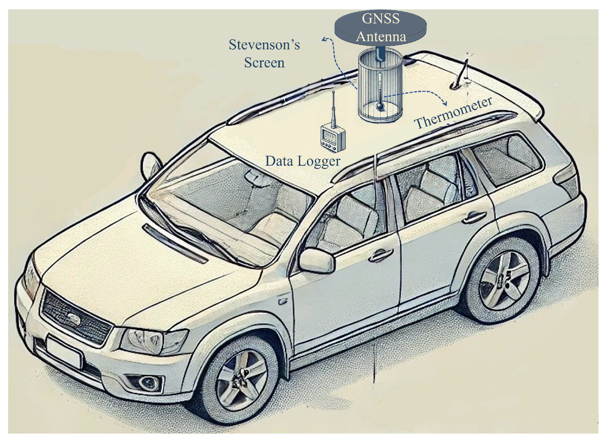
Figure 1. Schematic of the mobile air temperature measurement system.
Sustainability 18 01695 g001
Figure 2. Data Collection from Bologna (Italy): (a) Mobile path and air temperature, (b) Mobile path and land surface temperature, (c) Building information, and (d) Mobile path and vegetation.
Sustainability 18 01695 g002
Figure 3. Meteorological conditions between 19–25 March 2021 from ERA5 reanalysis and station data. (Top) Cloud cover (%) from ERA5, with the orange shaded area indicating the air temperature campaign and the red dashed line marking the Landsat overpass. (Middle) Wind speed (m/s) from the local station and ERA5 10 m data. (Bottom) Precipitation (mm) from the station and ERA5.
Sustainability 18 01695 g003
Figure 4. Block representation (buffer areas) for various data: (a) air temperature, (b) land surface temperature, (c) building density indicator, (d) floor to area ratio indicator, (e) mean building height indicator, and (f) presence of vegetation indicator.
Sustainability 18 01695 g004
Table 1. Pearson and Spearman’s Rank correlation matrix (The variables used in the analysis are MBH = Mean Building Height, BD = Building Density, FAR = Floor Area Ratio, PV = Proportion of Vegetation, AT = Air Temperature, and LST = Land Surface Tenmperature).
Spearman’s Rank
MBHBDFARPVATLST
PearsonMBH1.000.890.81−0.540.760.77
BD0.751.000.97−0.690.730.79
FAR0.730.961.00−0.680.790.73
PV−0.49−0.67−0.681.00−0.70−0.76
AT0.740.740.71−0.681.000.89
LST0.740.770.75−0.750.891.00
Table 2. Variance Inflation Factor (VIF), Condition Index (CI) and eigenvalue with variance decomposition results (The variables used in the analysis are MBH = Mean Building Height, BD = Building Density, FAR = Floor Area Ratio, and PV = Proportion of Vegetation).
VariableVIFPC1PC2PC3PC4
Eigenvalue-3.160.510.280.04
CI-1.002.483.348.87
MBH6.590.030.290.670.012
BD24.270.0070.0010.050.94
FAR24.620.0070.0010.060.93
PV2.300.0330.670.290.001
Table 3. Maximum Likelihood estimation results of the Spatial Lag Model (SLM) for air temperature (AT) and land surface temperature (LST).
Metric/VariableATLST
Mean Dependent Variable2.9412.38
S.D. Dependent Variable1.861.42
Pseudo R20.940.92
Spatial Pseudo R20.730.80
Log Likelihood−258.74−204.48
Sigma-square ML0.210.16
S.E. of regression0.460.40
AIC /SC525.49/540.88416.97/432.37
Constant (coef.)1.44 (p < 0.001)4.43 (p < 0.001)
CUDI (coef.)0.16 (p < 0.001)0.11 (p < 0.001)
PV (coef.)−2.56 (p < 0.001)−3.46 (p < 0.001)
Spatial Lag (W)0.80 (p < 0.001)0.74 (p < 0.001)
Impacts-CUDIDirect: 0.16/Indirect: 0.65/Total: 0.81Direct: 0.10/Indirect: 0.30/Total: 0.40
Impacts-PVDirect: −2.56/Indirect: −10.15/Total: −12.71Direct: −3.46/Indirect: −9.72/Total: −13.18
Residual Moran’s I0.10 (p = 0.003)0.12 (p < 0.001)
S.D.: Standard Deviation; ML: Maximum Likelihood; S.E.: Standard Error; AIC: Akaike Information Criterion; SC: Schwarz criterion.
Table 4. Results of spatial dependence diagnostics (the Lagrange Multiplier (LM) tests) for air temperature (AT) and land surface temperature (LST).
TestATLST
LM-Lag507.63343.20
Robust LM-Lag49.5455.04
LM-Error494.47316.67
Robust LM-Error36.3828.51
Disclaimer/Publisher’s Note: The statements, opinions and data contained in all publications are solely those of the individual author(s) and contributor(s) and not of MDPI and/or the editor(s). MDPI and/or the editor(s) disclaim responsibility for any injury to people or property resulting from any ideas, methods, instructions or products referred to in the content.