Liquidity-Based Tax Incentives and Corporate Green Innovation: Evidence from China’s VAT Credit Refund Policy

Abstract

Tax incentives are central to environmental policy, yet the innovation effects of liquidity-based fiscal instruments remain underexplored. This study asks whether China’s value-added tax (VAT) credit refund promotes corporate green innovation, and how firm governance and the policy environment condition that effect. Exploiting the 2018 industry-targeted pilot as a quasi-natural experiment, we estimate two-way fixed-effects difference-in-differences models on 25,259 firm-year observations for 4044 Chinese A-share listed firms over 2014–2021, measuring green innovation by invention-patent applications and defining treatment by industry eligibility. The refund raises green invention-patent applications by 17.0 percent, significant at the 1 percent level. A sequential decomposition is consistent with transmission through eased financing constraints and higher R&D investment. The effect is stronger where internal control quality is higher and pre-treatment financial slack is greater, and is absent where climate policy uncertainty (CPU) is high. Results survive removing control firms drawn in by the 2019 policy expansion, sector-by-year and province-by-year fixed effects, heterogeneity-robust estimators, and a triple difference on the innovation-quality margin. Fiscal liquidity complements governance quality and regulatory predictability rather than substituting for them.

1. Introduction

The transition toward a low-carbon economy depends heavily on corporate green innovation: technologies, products, and production processes that reduce pollution, conserve resources, and lower carbon intensity [1,2]. Green innovation combines two market failures rather than one. Like conventional research and development, it generates knowledge spillovers the innovating firm cannot fully capture [3]; unlike conventional R&D, it also generates environmental benefits that accrue to society rather than to the firm [4]. This double externality causes private green investment to fall short of the social optimum and provides the standard rationale for public intervention [5,6]. Governments have responded with a broad policy portfolio, and understanding which instruments move firm behavior, through what channels, and under what conditions is central to effective environmental policy design.

Among fiscal instruments, the tax system occupies a distinctive position. Most environmental tax incentives work by lowering the effective price of qualifying activities, for example through R&D super-deductions or accelerated depreciation for green equipment [7,8,9]. A different, less-examined class operates on the timing of cash flows rather than tax rates. China’s VAT credit refund policy belongs to this class. Firms that accumulate an uncredited input-VAT balance under China’s credit-invoice VAT, historically carried forward rather than refunded, effectively extend an interest-free loan to the government; the deferred claim exceeded RMB 1 trillion in 2018 and accounted for roughly 60 percent of the RMB 2.5 trillion in nationwide tax reductions and refunds by 2022 [10,11]. The reform converts this deferred claim into an immediate cash refund for firms in targeted industries, improving liquidity without altering the statutory tax burden [12].

Whether such a liquidity injection translates into green innovation is theoretically ambiguous. If green R&D is constrained by internal funds, as a large literature on financing constraints and innovation suggests [13,14], relaxing the cash constraint should raise innovation investment. But refunded cash is fungible and could instead fund dividends, debt repayment, or conventional capital expenditure; evidence shows the refund raises cash dividends [15] and cash holdings [16], so the policy might leave green technology largely untouched. Even where firms redeploy the cash, execution rests on the internal control environment, which governs how faithfully a stated intention becomes monitored expenditure [17,18]. Beyond the firm’s own governance, how uncertain the future of climate policy is plausibly shapes whether a windfall is worth committing to a long-gestation, irreversible green project at all.

This paper addresses that question by exploiting China’s 2018 VAT credit refund pilot as a quasi-natural experiment. In 2018, the authorities selected eighteen advanced-manufacturing, modern-service, and power-grid industries for one-time refunds of accumulated, uncredited input-VAT balances, before the policy was progressively broadened and made near-universal in 2022. This industry-targeted rollout generates plausibly exogenous variation in firms’ exposure to the liquidity shock. We estimate two-way fixed-effects difference-in-differences models with firm and year fixed effects on 25,259 firm-year observations covering 4044 firms over 2014–2021.

Green innovation is measured by patent applications, which are dated at filing and therefore record the moment a firm commits to a specific inventive project. Treatment is defined by industry eligibility, so the estimate is an intention-to-treat effect of eligibility rather than of refund receipt, and inference is clustered at the industry level, the level at which the pilot assigns eligibility.

We report three sets of findings. First, the refund raises green invention-patent applications both without firm controls (0.172, t = 3.215) and with a compact control set covering size, age, leverage, profitability, growth, and ownership concentration (0.157, t = 2.910, 95 percent CI [0.049, 0.264]); because the outcome is measured in logarithms, the preferred estimate corresponds to an increase of 17.0 percent (95 percent CI 5.1 to 30.2 percent). Second, a sequential decomposition is consistent with a coherent transmission chain: the refund eases financing constraints, which raises R&D investment intensity, which in turn raises green-invention applications; a Monte Carlo confidence interval for the indirect chain excludes zero. Third, the policy’s translation into innovation is conditional on the firm’s structural governance and on its external policy environment: it is strengthened by internal control quality, concentrates among firms with greater pre-treatment financial slack, and is absent in provinces with high climate policy uncertainty (CPU). The results strengthen when control firms drawn in by the 2019 expansion are removed, survive sector-by-year and province-by-year fixed effects, and are reproduced by the [19,20,21] estimators as well as by a triple difference on the innovation-quality margin.

This study makes three contributions. First, it extends the tax-and-innovation literature beyond price-based instruments, such as R&D super-deductions and investment tax credits, to a liquidity-based one. Because the refund accelerates the timing of a cash flow the firm already owned without changing statutory rates, it offers a setting in which liquidity effects on innovation can be studied with more limited confounding from tax-price changes than is typical of the literature; the channel we document is predominantly, rather than purely, liquidity-based, and we ground this distinction in the financing-constraints theory of investment [22,23].

Second, it advances the VAT-credit-refund literature, summarized in Section 2.2.2, which has documented effects on productivity, R&D spending, dividends, hiring, environmental ratings, and, in one recent study, a green-patenting result reported as a secondary channel within a broader carbon-emissions analysis [24]. We make green invention patenting the primary outcome rather than a downstream mechanism, and open the financing-to-innovation pathway with a formal sequential decomposition bounded by a Monte Carlo confidence interval.

Third, it identifies the conditions under which a fungible windfall becomes green technological output. Financing-constraints theory predicts that releasing a cash constraint raises constrained investment, but is silent on whether the released cash reaches any particular use. We locate the missing filter in the firm’s formal control architecture and in the credibility of the external climate policy environment, showing that fiscal liquidity complements rather than substitutes for governance quality and regulatory predictability.

The remainder of this paper proceeds as follows. Section 2 describes the institutional background, reviews the related literature, and develops the hypotheses. Section 3 details the sample, variable measurement, and empirical specification. Section 4 reports the main results, and Section 5 reports the identification and robustness analysis. Section 6 discusses the findings and concludes.

2. Institutional Background, Literature Review, and Hypothesis Development

2.1. Institutional Background

2.1.1. The VAT Credit Refund Mechanism

China operates a credit-invoice value-added tax under which a taxpayer’s liability equals output tax, VAT collected on sales, minus input tax, VAT paid on purchases. When input tax exceeds output tax, common for firms making large upfront investments in equipment, materials, or R&D inputs, the shortfall is recorded as an uncredited input-VAT balance. Historically, this balance could not be refunded; it could only be carried forward to offset future output VAT. Economically, the accumulated balance functions as an interest-free loan from the firm to the tax authority: the firm has already remitted cash on its purchases but cannot recover it until it generates sufficient future output VAT to absorb the credit [16]. For capital- and innovation-intensive firms, these balances tie up working capital precisely when liquidity is most valuable for financing long-gestation projects such as green R&D [24].

The VAT credit refund policy reverses this by refunding the uncredited balance in cash. The refund does not change the firm’s total tax liability over time; it accelerates the recovery of input VAT the firm was already entitled to credit [15]. This makes it a plausibly exogenous liquidity shock: it improves the firm’s cash position and reduces reliance on external finance while leaving the statutory tax burden, and the tax price of any input, unchanged [12]. Tax-price invariance is not the same as invariance of the effective cost of investment. Improved liquidity can still move the shadow cost of internal capital and the marginal investment threshold a project must clear, and may indirectly ease borrowing capacity or terms with lenders. The refund therefore need not leave every margin of the investment decision untouched even though it leaves relative prices unchanged. This institutional feature is nonetheless central to identification: because the refund alters the timing of a cash flow the firm already owned rather than the price of any input, an innovation response is more plausibly attributed to a financing channel than to a price channel, a distinction most of the tax-incentive literature cannot draw so cleanly.

2.1.2. Policy Evolution and the 2018 Pilot

China’s refund regime evolved in three stages. In June 2018 the Ministry of Finance and the State Administration of Taxation jointly launched an industry-targeted pilot: firms in eighteen defined advanced-manufacturing, high-technology, and power-grid industries became eligible for a one-time refund of accumulated uncredited input-VAT balances (Cai-Shui (2018) No. 70). Eligibility was defined by industry classification at the two-digit level, generating cross-sectional variation in exposure to the liquidity shock that was outside the control of any individual firm. In 2019, the scope was broadened and an incremental-refund mechanism introduced for a wider set of taxpayers. In 2022, the policy became a near-universal program covering essentially all qualifying enterprises and refunding both incremental and stock balances on an accelerated schedule (MOF-STA Announcement (2022) No. 14).

Identification centers on the 2018 pilot, which offers the cleanest comparison: firms in the eighteen eligible industries versus otherwise similar firms in industries not covered by the pilot. Two features of this design require explicit treatment.

First, eligibility is not receipt. A firm in an eligible industry obtained a refund only if it held an accumulated uncredited balance and claimed against it, and 44.6 percent of eligible firms in our sample did so. Because take-up is a firm decision plausibly correlated with unobserved determinants of innovation, we define treatment by industry eligibility and interpret the headline estimate as an intention-to-treat effect, documenting compliance in Section 4.2.1.

Second, the 2019 expansion partially contaminates the control group. Firms outside the 2018 pilot industries became eligible for incremental refunds from 2019, so the post-2019 contrast is not between exposed and wholly unexposed firms. We identify which control firms were drawn into eligibility and in which year, and Section 5.1 reports the estimate after dropping them, after censoring their post-contamination observations, on a clean pre-expansion window, and with the two reforms modelled as separate treatment cohorts.

The 2022 universal reform is institutional context rather than a second estimable experiment, since once the policy became universal no untreated comparison group remains within the listed-firm sample.

2.2. Related Literature

This section situates this study within five strands: tax incentives and corporate innovation; the economic consequences of China’s VAT credit refund; financing constraints and green innovation; corporate governance, internal control, and innovation; and the institutional and policy-uncertainty environment for corporate investment.

2.2.1. Tax Incentives, Liquidity, and Corporate Innovation

A substantial literature establishes that fiscal incentives shape corporate investment and innovation. The dominant mechanism studied is price-based: by lowering the after-tax cost of qualifying activities, instruments such as R&D super-deductions, tax credits, and accelerated depreciation raise the marginal return to investment and thereby its level [7,8,9]. The empirical consensus is that such instruments stimulate R&D and capital formation, though magnitudes vary with firm characteristics and with whether the incentive is salient and certain.

A second mechanism, less studied but increasingly recognized, operates through liquidity rather than price. Where firms face financing constraints, the timing and availability of internal cash can independently determine investment even holding the cost of capital fixed [22,25]. The theoretical foundation is well established: because outside investors cannot fully verify the quality of a firm’s investment opportunities, external finance carries an information-asymmetry premium over internal funds [23,26], so a dollar of internal cash is not a perfect substitute for a dollar raised externally, and firms follow a financing pecking order favoring internal funds. Tax policy can relax this constraint directly: a refund or deferral that places cash in the firm’s hands eases the working-capital position and substitutes for costly external finance. The authors of [9] show that investment responses to tax incentives concentrate in financially constrained firms and are sensitive to whether the incentive generates immediate cash flow, underscoring that the cash-flow timing of a tax instrument, not only its present value, matters for real behavior.

Two related channels are worth separating. A pure timing, or liquidity, effect delivers cash earlier without altering its total present value or the price of any input. A financing-cost effect instead changes the effective cost of capital itself, for example by improving collateral position, credit rating, or bargaining leverage with lenders. The VAT credit refund is designed primarily as a timing instrument, but because improved liquidity can also ease borrowing terms, some part of any observed effect may operate through this second channel. The two are not perfectly separable in practice, which is why we describe the refund’s effect as predominantly, rather than purely, liquidity-based.

2.2.2. Economic Consequences of the VAT Credit Refund

A fast-growing body of work, almost entirely focused on China, examines the corporate consequences of the VAT credit refund. On the input side, the refund raises R&D expenditure [11] and supports hiring and human-capital accumulation [27,28]; it also raises total factor productivity [10]. On the financial-policy side, refunded cash has been linked to higher cash dividends [15] and larger cash holdings [16], and to lower stock-price crash risk [29]. On the strategic side, the refund has been associated with outward foreign direct investment [30]. A smaller set of studies reaches toward environmental outcomes: the authors of [24] find that the refund reduces firms’ carbon emissions and emissions intensity, reporting a rise in green invention-patent counts as one of three parallel mechanisms behind that result, and [12] link the refund to broader environmental ratings.

Three gaps motivate our study. First, only one study links the refund to green invention patents, and there as a secondary mechanism en route to a carbon-emissions outcome rather than as the object of dedicated investigation. Green technological output examined as a primary outcome, and the conditions under which the refund translates into it, therefore remains largely open. Second, existing studies typically report a reduced-form effect without formally testing the full transmission mechanism; where a mechanism is examined it either stops at a single mediator [11] or reports multiple channels descriptively rather than as a jointly tested sequential chain [24]. Third, the literature treats the firm as a largely passive conduit through which cash mechanically becomes investment. Because refunded cash is fungible and can be paid out as dividends rather than reinvested, whether it reaches long-gestation green projects should depend on the firm’s internal control environment and on the institutional and policy environment beyond its boundary, in particular, how uncertain the future direction of climate policy is [31].

2.2.3. Financing Constraints and Green Innovation

Green innovation is especially vulnerable to financing constraints. Like R&D in general, it is intangible, uncertain, long-gestating, and poorly collateralized, features that amplify information asymmetry between managers and outside financiers [23,26] and make external finance costly and rationed [13,14]. Green innovation compounds these features with a second externality, environmental benefits the innovating firm cannot fully appropriate, which further depresses private returns relative to social returns [5,6] and makes green projects the first casualty when internal funds tighten. Internal cash flow is therefore a particularly important funding source for green projects, and instruments that relax the cash constraint should disproportionately benefit them. We measure financing constraints with the SA index of [32], which relies only on firm size and age, deliberately avoiding endogenous financial ratios, and use it both as the mediating variable in our mechanism tests and, on its pre-treatment value, as the internal-environment heterogeneity split in Section 4.5.

2.2.4. Corporate Governance, Internal Control, and Innovation

A separate literature roots managerial behavior toward discretionary cash in agency theory. Reference [18] shows that free cash flow, cash beyond what is needed to fund positive-net-present-value projects, is a particular locus of managerial discretion, prone to diversion toward perquisite consumption, empire-building, or earnings-smoothing uses that serve managers’ private interests rather than shareholder value. A firm’s internal control system, spanning risk assessment, control activities, information and communication, and monitoring, is the primary structural mechanism through which this discretion is narrowed [33]. It imposes structured capital-budgeting and project-approval processes and improves the reliability of information used to evaluate long-gestation, hard-to-verify projects such as green R&D. In the Chinese context, internal control quality is most commonly proxied by the internal control and risk management index compiled by DIB (Shenzhen Dibo Enterprise Risk Management Technology Co., Shenzhen, China), used extensively in the accounting and finance literature [33]. We draw on this literature to motivate internal control quality as a structural moderator of the refund-to-innovation link.

2.2.5. Institutional Environment, Policy Uncertainty, and Corporate Investment

A third relevant literature examines how the policy environment beyond the firm’s boundary shapes corporate investment. Ref. [34] shows that heightened uncertainty raises the option value of waiting and induces firms to pause investment and hiring until uncertainty resolves; ref. [35] formalizes this real-options logic for investments, like green R&D, that are costly to reverse. Applied to environmental regulation, the news-based CPU index of [36], constructed at a provincial level from Chinese-language news text, provides a direct, time-varying proxy for how uncertain the future direction of environmental regulation appears in a given province and year. Because green R&D is long-gestation and largely irreversible once undertaken, and because recent firm-level evidence in China favors deferral over strategic positioning as the dominant response to CPU [37], we expect CPU to dampen the conversion of a liquidity windfall into green invention, a possibility that has not previously been tested for the VAT credit refund or any comparable liquidity-based environmental instrument.

2.3. Hypothesis Development

The financing-constraints theory of investment predicts that an exogenous increase in internal funds raises investment in activities rationed by the availability of internal funds. What it does not predict is that the released cash reaches any particular use. Refunded cash is fungible—the canonical question of what firms do with a windfall [38]—and the VAT-refund literature shows it flowing to dividends [15] and cash holdings [16] as readily as to R&D [11]. What is missing is a theory of the filter between liquidity and use. We locate that filter in two places: the firm’s formal control architecture, which governs whether an investment intention becomes monitored expenditure, and the credibility of the external climate policy environment, which governs whether a long-gestation, irreversible green commitment is worth making at all.

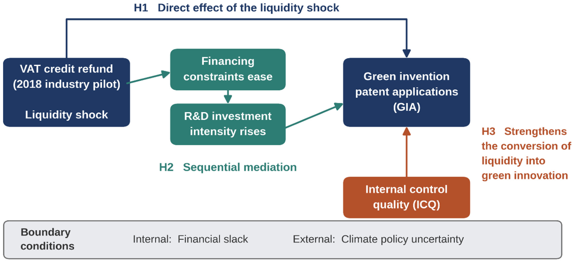
This review yields three claims: one establishing that the policy affects green innovation at all, one specifying the channel, and one identifying the structural governance condition on which the channel depends. Section 4.5 additionally examines whether the baseline effect is conditioned by the internal and external environment in which a firm is embedded; we treat this as a corollary of the mechanism established in H1 and H2 rather than as an independent hypothesis. Figure 1 summarizes the conceptual framework.

2.3.1. Baseline Effect

Our point of departure is the financing-constraints theory of investment: because external funds carry an information-asymmetry premium over internal funds [23,26], an exogenous increase in internal cash should raise investment in activities otherwise rationed by the availability of internal funds. Green innovation is a paradigm case. It is intangible and poorly collateralized, so it cannot easily be pledged to secure external finance [14]; it is uncertain and long-gestating, so its expected payoff is difficult for outside investors to verify ex ante [26]; and it generates environmental benefits the firm cannot fully capture, which depresses the private return relative to the social return and makes it an easy target for cuts when funds are scarce [5,6]. The VAT credit refund relaxes this constraint through a channel distinct from price: it converts a deferred, non-interest-bearing claim into immediate cash without changing the marginal cost of R&D, capital, or labor.

Hypothesis 1 (H1).

The VAT credit refund increases the green innovation output of firms in eligible industries relative to firms in ineligible industries.

2.3.2. Mechanism: A Sequential Financing-to-Innovation Chain

H1 is a reduced-form claim about the ultimate outcome; it is silent on how the refund gets there. The financing-constraints logic implies a specific, ordered channel rather than a direct jump from cash to patents. Because the refund is a predominantly liquidity-based injection that leaves relative prices unchanged, its most proximate consequence should be observed on the firm’s funding position itself: measured financing constraints should ease. Improved liquidity should then be deployed into the investment most proximate to green output, R&D. Under the pecking-order logic of [23], firms prefer to fund discretionary, hard-to-finance investment with internal funds before turning to costly external finance, so an exogenous easing of financing constraints should raise R&D investment intensity, the input into which green patents are eventually converted. Higher R&D intensity should in turn raise green innovative output.

These three links are not independent hypotheses to be tested in isolation; they describe a single proposed pathway. We state the mechanism as one compound hypothesis and test it with a sequential decomposition together with a Monte Carlo confidence interval for the compound indirect effect. Financing constraints, R&D investment, and innovation are plausibly jointly determined, and our estimates cannot establish the temporal ordering of a chain in which all three respond to the same shock. H2 is therefore a claim about statistical consistency with the proposed pathway rather than about sequential structural causality.

Hypothesis 2 (H2).

The effect of the VAT credit refund on green innovation is consistent with transmission through a sequential channel: the refund eases financing constraints, which raises R&D investment intensity, which in turn raises green innovation.

2.3.3. Moderation: The Structural Governance Filter

H1 and H2 describe a conversion of liquidity into innovation, but that conversion passes through the firm’s formal control environment. Whether a manager chooses to redirect a windfall toward long-horizon green investment is not the only determinant of the outcome: the control architecture governs how faithfully any intention is translated into monitored, well-executed investment. Because free cash flow is a particular locus of managerial discretion [18], robust internal controls narrow this discretion [33]. Internal controls impose structured capital-budgeting and project-approval processes, improve the reliability of the information managers and boards use to evaluate long-gestation, hard-to-verify projects, and raise the probability that a discretionary cash inflow is captured by, rather than diverted from, the firm’s stated investment priorities [39]. A well-controlled firm should therefore be better equipped to convert an approved R&D intention into monitored expenditure and, eventually, a filed patent application.

This is not a claim that stronger internal controls are unambiguously beneficial: the same structured approval processes that improve monitoring fidelity can add bureaucratic friction and narrow managerial flexibility [40]. H3 is conditional on the specific interaction we estimate between internal control quality and the conversion of this particular liquidity windfall into green R&D.

Hypothesis 3 (H3).

Internal control quality strengthens the positive effect of the VAT credit refund on green innovation.

2.3.4. Internal and External Boundary Conditions

Beyond this governance mechanism, the same liquidity logic implies that the size of the effect should depend on the firm’s capacity to redeploy the windfall and on whether redeployment is worth undertaking. A firm’s pre-treatment financial slack determines how much of a windfall it can direct toward new projects rather than balance-sheet repair [41]. Climate-policy uncertainty operates through a different channel: because green R&D is a long-gestation, largely irreversible commitment whose payoff depends on the future stringency and stability of environmental regulation, the real-options logic of investment under uncertainty [35] implies that a firm facing high uncertainty about the future direction of climate policy has an incentive to defer such commitments and preserve financial flexibility, even when internal liquidity is momentarily abundant [31,34].

3. Materials and Methods

3.1. Sample and Data

Our sample comprises Chinese A-share listed firms observed between 2014 and 2021, the window surrounding the 2018 pilot; the period ends in 2021 because the 2022 reform extended the refund to essentially all firms and removed the control group. Following standard practice, we exclude financial-sector firms, firms under special-treatment (ST/*ST) status, and observations with missing values on the core variables, and we drop singleton firm or year observations that contribute no within-firm or within-year variation to the two-way fixed-effects model. After this screening, we retain 25,259 firm-year observations on 4044 firms across 76 two-digit industries and 31 provinces, of which 35.0 percent are DID = 1 observations.

All continuous variables are winsorized at the 1st and 99th percentiles. This applies to the continuous control variables, the mechanism variables (SA, CashFlow, RDRatio), and the moderating and heterogeneity variables (ICQ, CPU, financial slack). Count-based outcome variables are not winsorized.

Firm financials, ownership, and governance variables, together with the treatment indicators built from the 2018 pilot industry catalogue, are drawn from the CSMAR database. Green invention-patent application counts are collected from the China National Intellectual Property Administration and classified following the World Intellectual Property Organization (WIPO) Green Inventory. Internal control quality scores come from the DIB internal control and risk management database, a widely used proxy in the Chinese accounting and finance literature for the design and operating effectiveness of a firm’s internal control system [33]; we standardize the raw index to mean zero and unit variance so that its interaction coefficient is interpretable per one-standard-deviation change. Provincial CPU comes from the news-based index of [36], which applies deep-learning text classification to more than 1.7 million articles from six major Chinese newspapers; the index has been used to measure CPU in China in prior work [42]. We obtain the series from the ISETS Energy Finance Network.

3.2. Variable Definitions

Table 1. Variable definitions. Definitions and construction of the dependent variable, key explanatory variables, control variables, mechanism variables, the moderation variable, and boundary-condition variables.

Variable	Symbol	Definition
Panel A: Dependent Variable
Green Innovation	GIA	Natural logarithm of one plus the count of green invention-patent applications.
Panel B: Key Explanatory Variables
Difference-in-Differences	DID	Interaction term Eligible × Post; equals 1 for pilot-industry firms in 2018 and later, and 0 otherwise. Identifies an intention-to-treat effect of industry eligibility.
Eligible Industry	Eligible	Dummy equal to 1 if the firm’s two-digit CSRC industry is one of the eighteen named in the June-2018 pilot (Cai-Shui (2018) No. 70), and 0 otherwise.
Post-Treatment Period	Post	Dummy equal to 1 in 2018 and every subsequent year, and 0 otherwise.
Panel C: Control Variables
Firm Size	Size	Natural logarithm of total assets.
Firm Age	Age	Natural logarithm of one plus firm age (years since listing).
Book Leverage	Lev	Total liabilities divided by total assets.
Return on Assets	ROA	Net profit divided by total assets.
Revenue Growth	Growth	Growth rate of operating revenue.
Ownership concentration	Top1	Shareholding percentage of the largest shareholder.
Panel D: Mechanism Variables
Financing Constraint	SA	SA = −0.737 × Size + 0.043 × Size2 − 0.040 × Age. Higher values indicate greater financing constraints.
Operating Cash Flow	CashFlow	Net operating cash flow scaled by total assets.
R&D Intensity	RDRatio	R&D expenditure scaled by operating revenue.
Panel E: Moderation Variable
Internal Control Quality	ICQ	Standardized DIB Internal Control Index score; higher values reflect stronger internal control design and implementation.
Panel F: Boundary-Condition Variables
Financial Slack	Slack	Indicator equal to 1 if the firm’s pre-treatment (2014–2017) average SA index is below the sample median.
Climate Policy Uncertainty	CPU	Provincial climate policy uncertainty index of [36], evaluated at the pre-treatment provincial average.

defines all variables.

The dependent variable is GIA, the natural logarithm of one plus the count of green invention-patent applications. Applications are dated at filing, so the measure records the moment a firm commits to a specific inventive project and bears the cost of documenting it, which is the decision the liquidity shock is hypothesized to move. Invention patents, which require substantive examination for novelty and inventive step, are our focus rather than utility models, which do not; Section 5.3 reports a triple difference between the two that isolates the innovation-quality margin.

The key explanatory variables are Eligible, an indicator equal to one for firms in one of the eighteen 2018-pilot industries; Post, equal to one in 2018 and every subsequent year; and their interaction, DID, the coefficient of interest throughout. Because eligibility is defined by industry classification while receipt of a refund additionally required an accumulated uncredited balance and a claim, DID identifies an intention-to-treat effect of industry eligibility. Take-up within eligible industries is a firm decision plausibly correlated with unobserved determinants of innovation, whereas industry membership is fixed within our panel, which makes eligibility the more credible source of variation.

The baseline control vector comprises firm size, age, leverage, return on assets, revenue growth, and the shareholding percentage of the largest shareholder. We report the baseline both with and without this vector as alternative specifications; controls measured contemporaneously with the outcome may themselves respond to the treatment, so their addition is not a robustness test.

Three mechanism variables operationalize H2: the SA financing-constraint index of [32], computed as SA = −0.737 × Size + 0.043 × Size² − 0.040 × Age, with higher values indicating greater constraints; operating cash flow scaled by total assets (CashFlow); and R&D expenditure scaled by operating revenue (RDRatio).

One moderation variable operationalizes H3: internal control quality (ICQ), the standardized DIB internal control index.

Two further variables operationalize the boundary-condition analysis in Section 4.5: the firm’s pre-treatment (2014–2017) average SA index, used to split the sample into higher- and lower-financial-slack subsamples, and the province-level CPU index, evaluated at its pre-treatment provincial average. Both splits are formed on pre-treatment values so that the splitting variable cannot itself be affected by the policy.

3.3. Empirical Specification

3.3.1. Baseline Difference-in-Differences

We estimate the effect of the refund on green invention-patent applications with a two-way fixed-effects DID model:

GIA_i,_t = β₀ + β₁·DID_i,_t + γ′X_i,_t + μ_i + λ_t + ε_i,_t

(1)

where DID_i,_t = Eligible_i × Post_t; X_i,_t is a compact vector of firm controls (Size, Age, Lev, ROA, Growth, and Top1); and μ_i and λ_t are firm and year fixed effects. The coefficient of interest is β₁.

Standard errors are clustered at the industry level (two-digit CSRC, 76 clusters), the level at which the pilot assigns eligibility: firms sharing an industry share their treatment assignment and any shock correlated with it. Section 5.4 confirms the result under a wild cluster bootstrap and under randomization inference over industry eligibility.

3.3.2. Chain-Mediation Specification

We test the sequential channel underlying H2 in stages. First, we regress each of the three mechanism variables, SA, CashFlow, and RDRatio, on DID, controls, and fixed effects; because SA is mechanically a function of Size and Age, we exclude those two from the control set in the SA regression only. We then estimate a chain of the form DID → SA → RDRatio → GIA: path a regresses SA on DID and controls; path b regresses RDRatio on SA, DID, and the full control vector; and path c regresses GIA on RDRatio, DID, and the full control vector, so that the direct effect of DID net of the mediating path is recovered from path c. We compute the compound indirect effect as a × b × c and construct its confidence interval by Monte Carlo simulation [43] with 200,000 draws from the asymptotic sampling distributions of the path estimates.

A confidence interval that excludes zero establishes that the estimated product is inconsistent with a null indirect path, not that the causal ordering runs in the direction imposed. We read the result as statistically consistent with the proposed pathway rather than as identification of a sequential mechanism.

3.3.3. Moderation

We test the structural governance condition (H3) by augmenting Equation (1) with the moderator and its interaction with DID:

GIA_i,_t = β₀ + β₁ · DID_i,_t + β₂ · (DID × ICQ)_i,_t + β₃ · ICQ_i,_t + γ′X_i,_t + μ_i + λ_t + ε_i,_t

(2)

where ICQ is the standardized internal control index, so β₂ is the change in the DID coefficient per one-standard-deviation increase in internal control quality. A positive β₂ supports H3.

3.3.4. Boundary Conditions

We split the sample by pre-treatment financial slack, at the sample median of each firm’s 2014–2017 average SA index; because SA is decreasing in financial slack, the below-median subsample is labeled high financial slack. We apply the same pre-treatment-average logic to each firm’s provincial CPU index. For each split, we estimate Equation (1) separately on each subsample and report a Chow-type test in which every control variable, not only DID, is interacted with the subsample indicator, so that the reported p-value tests equality of the treatment slope across subsamples.

4. Results

4.1. Descriptive Statistics

Table 2. Summary statistics and correlations. Descriptive statistics (Panel A) and pairwise Pearson correlations (Panel B) for the main variables. All continuous variables are winsorized at the 1st and 99th percentiles; count-based outcome variables are not winsorized. *** and ** denote statistical significance at the 1% and 5% levels, respectively.

Panel A: Descriptive statistics
Name	Obs.	Mean	SD	Min	p25	p50	p75	Max
GIA	25,259	0.677	1.108	0.000	0.000	0.000	1.099	7.432
DID	25,259	0.350	0.477	0.000	0.000	0.000	1.000	1.000
SA	25,259	−3.857	0.247	−4.512	−4.020	−3.853	−3.694	−3.225
CashFlow	25,259	0.048	0.068	−0.155	0.010	0.047	0.088	0.239
RDRatio	25,259	0.043	0.048	0.000	0.008	0.034	0.054	0.271
ICQ	23,605	0.001	0.999	−4.329	−0.093	0.228	0.473	1.275
Size	25,259	22.262	1.297	19.954	21.331	22.078	22.993	26.273
Age	25,259	2.970	0.295	2.197	2.773	2.996	3.178	3.584
Lev	25,259	0.419	0.204	0.058	0.255	0.409	0.567	0.908
ROA	25,259	0.040	0.070	−0.253	0.014	0.040	0.074	0.218
Growth	25,259	0.166	0.379	−0.583	−0.023	0.107	0.270	2.037
Top1	25,259	0.336	0.146	0.085	0.222	0.313	0.431	0.737
CPU	25,259	0.483	0.196	0.208	0.390	0.465	0.536	1.543
Panel B: Correlation matrix
	(1)	(2)	(3)	(4)	(5)	(6)	(7)	(8)
GIA	1.000
DID	0.198 ***	1.000
Size	0.399 ***	−0.111 ***	1.000
Age	0.015 **	0.043 ***	0.191 ***	1.000
Lev	0.183 ***	−0.116 ***	0.508 ***	0.187 ***	1.000
ROA	0.007	0.022 ***	−0.019 ***	−0.123 ***	−0.394 ***	1.000
Growth	0.031 ***	0.004	0.043 ***	−0.063 ***	0.006	0.271 ***	1.000
Top1	0.023 ***	−0.135 ***	0.187 ***	−0.076 ***	0.034 ***	0.156 ***	−0.006	1.000

, Panel A reports summary statistics for the estimation sample. GIA is right-skewed with a substantial mass at zero, as is typical of patent data: the median firm-year records no green invention-patent application, while the maximum reaches 7.432 in logged terms, reflecting a small number of highly prolific patenting firms. Among the controls, mean firm size is 22.262, mean leverage is 0.419, mean return on assets is 0.040, mean revenue growth is 0.166, and the largest shareholder holds 33.6 percent of shares on average, all broadly typical of the Chinese A-share listed population over this period [44].

Because ICQ enters as a moderator in a specification with firm fixed effects, its within-firm variation matters for whether the interaction is identified. Its overall standard deviation of 0.999 decomposes into 0.765 within firms and 0.695 between firms, so internal control quality varies substantially over time within the same firm.

The highest correlation among the control variables is between Size and Lev (0.508), consistent with larger firms carrying more debt; all other pairwise correlations among controls are well under the 0.8 threshold conventionally used to flag multicollinearity concern, and variance inflation factors do not exceed 1.72 for any regressor (Appendix A 

Table A1. Variance inflation factors. Variance inflation factors for the baseline specification of Table 3, column 2.

Variable	VIF
DID	1.037
Size	1.496
Age	1.075
Lev	1.724
ROA	1.406
Growth	1.106
Top1	1.094

). DID correlates only modestly with each control, consistent with the industry-based assignment of treatment being largely orthogonal to firm-level financial characteristics.

4.2. Baseline Effect on Green Invention-Patent Applications

Table 3. Baseline regressions. Two-way fixed-effects estimates of the effect of the VAT credit refund policy (DID) on green invention-patent applications (GIA), without (column 1) and with (column 2) firm-level control variables. DID is the intention-to-treat interaction of industry eligibility with the post-2018 indicator. Firm and year fixed effects are included in both columns; t-statistics based on industry-clustered standard errors are reported in parentheses. *** denote statistical significance at the 1% level.

	(1) Without Controls	(2) with Controls
Variable	GIA	GIA
DID	0.172 *** (3.215)	0.157 *** (2.910)
Size		0.296 *** (7.697)
Age		−0.155 (−0.617)
Lev		−0.194 *** (−3.303)
ROA		−0.144 (−1.217)
Growth		−0.004 (−0.277)
Top1		0.123 (1.479)
Firm FE	Y	Y
Year FE	Y	Y
Observations	25,259	25,259
R-squared	0.787	0.793

presents the baseline DID estimates for GIA, without firm controls in column (1) and with the compact control vector in column (2). The coefficient on DID is 0.172 (t = 3.215) without controls and 0.157 (t = 2.910) with controls; both are significant at the 1 percent level. For the preferred specification in column (2), the standard error is 0.054, the exact p-value is 0.0048, and the 95 percent confidence interval is [0.049, 0.264]. Among the controls, firm size is a strong positive predictor of green-patent applications (0.296, t = 7.697) and leverage carries a negative and significant coefficient (−0.194, t = −3.303). Table 3 supports H1.

In economic terms, because GIA is the natural logarithm of one plus the application count, the percentage effect is exp(β) − 1 rather than the coefficient itself; this transformation is applied to every percentage effect reported in the paper. The column (2) estimate therefore implies that eligibility raises green invention-patent applications by 17.0 percent (95 percent CI 5.1 to 30.2 percent), or approximately 0.9 additional applications at the estimation-sample mean of 5.40 applications per firm-year. Benchmarked against price-based R&D tax incentives, this sits within the plausible range. Incentives targeted narrowly at small, financially constrained firms have produced far larger responses: exploiting a UK size-based eligibility threshold for R&D tax relief, [45] find that R&D spending roughly doubled and patenting rose by about 60 percent among newly eligible firms. Broader, less-targeted price-based instruments produce more modest effects: cross-country evidence surveyed by [7] implies that a 10 percent fall in the user cost of R&D raises the long-run level of R&D by under 10 percent. Our effect is smaller than the response of size-selected, constrained firms to a direct price subsidy, which is unsurprising given that the VAT credit refund does not select on firm size or ex ante constraint status and does not change the price of R&D at all.

4.2.1. Compliance and Treatment Intensity

Because DID is defined by industry eligibility rather than refund receipt, the estimate in Table 3 is an intention-to-treat effect. Of the 2490 firms in eligible industries, 44.6 percent are observed to receive a refund in the post-2018 period. Eligibility raises the refund actually received, scaled by assets (0.00060, t = 1.918), and the post-2018 mean refund intensity is 0.00872 among eligible firms, compared with 0.00478 among control firms.

Estimates under alternative treatment definitions are correspondingly larger: 0.180 (t = 5.646) when treatment is defined as eligibility combined with observed refund receipt, and 0.108 (t = 4.341) under a sustained-take-up definition requiring receipt in at least two years. A continuous-intensity specification, replacing the binary interaction with excess refund scaled by assets, yields 7.654 (t = 2.790). The ratio between the take-up and intention-to-treat estimates is approximately what imperfect compliance would imply, consistent with the intention-to-treat estimate being diluted by non-claiming eligible firms rather than measuring a different phenomenon. Full results are omitted to save space and are available from the corresponding author on request.

4.2.2. Dynamic Effects and the Parallel-Trends Assumption

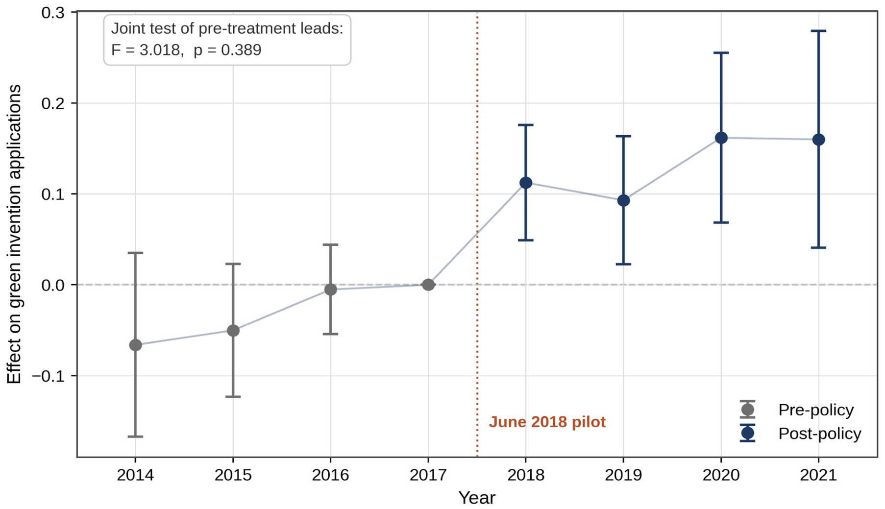
Figure 2 and Appendix A 

Table A2. Dynamic event-study coefficients. Coefficients on eligible-industry × year interactions with 2017 as the reference year, from the specification plotted in Figure 2. Firm and year fixed effects and the baseline control vector are included; standard errors are clustered at the industry level. The joint test of all pre-treatment leads gives F = 3.018, p = 0.389. *** and ** denote statistical significance at the 1% and 5% levels, respectively.

Year	Coefficient	Std. Error	t	95% CI
2014	−0.066	0.051	−1.304	[−0.167, 0.035]
2015	−0.050	0.037	−1.368	[−0.123, 0.023]
2016	−0.005	0.025	−0.210	[−0.054, 0.044]
2017	0 (reference)	—	—	—
2018	0.112 ***	0.032	3.524	[0.049, 0.176]
2019	0.093 **	0.035	2.627	[0.023, 0.164]
2020	0.162 ***	0.047	3.450	[0.068, 0.255]
2021	0.160 ***	0.060	2.673	[0.041, 0.279]

report the event-study specification, which replaces the single DID indicator with a full set of eligible-industry × year interactions. We use 2017 as the reference year because it is the last complete year before the June-2018 pilot; taking 2018 would place partially treated months in the reference period.

The three pre-treatment coefficients are small, individually insignificant, and shrink monotonically toward zero as treatment approaches: −0.066 in 2014, −0.050 in 2015 and −0.005 in 2016. A joint test fails to reject the null that all pre-treatment leads are zero (F = 3.018, p = 0.389). All four post-treatment coefficients are individually significant, rising from 0.112 (t = 3.524) in 2018 to 0.160 (t = 2.673) in 2021, and the effect is already present in the year of the policy. A firm receiving a refund in the second half of 2018 can prepare and file a patent application within months, so the 2018 coefficient is intelligible, though attenuated by the partial-year nature of treatment; Section 5.1 reports three alternative treatments for that year.

4.3. Mechanism Tests

Table 4. Mechanism analysis. Estimates of the policy’s effect on the three mechanism variables—financing constraints (SA), operating cash flow (CashFlow), and R&D investment intensity (RDRatio)—each regressed on DID and the baseline controls, with firm and year fixed effects. Size and Age are omitted from column (1) because SA is a deterministic function of both. t-statistics based on industry-clustered standard errors are reported in parentheses. *** and ** denote statistical significance at the 1% and 5% levels, respectively.

	(1)	(2)	(3)
Variable	SA	CashFlow	RDRatio
DID	−0.024 *** (−3.649)	0.006 ** (2.462)	0.003 ** (2.517)
Size		−0.007 *** (−3.664)	0.003 ** (2.315)
Age		−0.001 (−0.037)	−0.014 *** (−2.704)
Lev	−0.035 ** (−2.564)	0.006 (0.759)	−0.023 *** (−5.216)
ROA	−0.001 (−0.141)	0.232 *** (11.398)	−0.077 *** (−6.825)
Growth	−0.008 *** (−5.003)	−0.000 (−0.225)	−0.006 *** (−5.013)
Top1	0.070 *** (4.139)	−0.009 (−1.108)	0.001 (0.151)
Firm FE	Y	Y	Y
Year FE	Y	Y	Y
Observations	25,259	25,259	25,259
R-squared	0.975	0.492	0.881

reports the effects of the refund on the three mechanism variables. The refund significantly eases the SA index (−0.024, t = −3.649; because SA is increasing in financing constraints, a negative coefficient indicates looser constraints), raises operating cash flow (0.006, t = 2.462), and raises R&D investment intensity (0.003, t = 2.517). All three carry the sign the mechanism predicts.

Table 5. Chain mediation analysis. Panel A reports the three path regressions underlying the decomposition DID → SA → RDRatio → GIA, with firm and year fixed effects. Panel B summarizes the results, including the point estimate and 95 percent Monte Carlo confidence interval (200,000 draws) for the indirect effect. t-statistics based on industry-clustered standard errors are reported in parentheses. *** and ** denote statistical significance at the 1% and 5%, levels, respectively.

Panel A: Chain mediation path
	(1)	(2)	(3)
Variable	Path a: DID → SA	Path b: SA → RDRatio	Path c: RDRatio → GIA
DID	−0.024 *** (−3.649)	0.003 ** (2.261)	0.153 *** (2.833)
SA		−0.014 ** (−2.624)
RDRatio			1.316 *** (3.600)
Size		0.003 ** (2.249)	0.293 *** (7.624)
Age		−0.017 *** (−3.029)	−0.136 (−0.547)
Lev	−0.035 ** (−2.564)	−0.023 *** (−5.371)	−0.164 *** (−2.899)
ROA	−0.001 (−0.141)	−0.077 *** (−6.853)	−0.042 (−0.366)
Growth	−0.008 *** (−5.003)	−0.006 *** (−5.090)	0.004 (0.243)
Top1	0.070 *** (4.139)	0.001 (0.316)	0.122 (1.468)
Firm FE	Y	Y	Y
Year FE	Y	Y	Y
Observations	25,259	25,259	25,259
R-squared	0.975	0.881	0.794
Panel B: Chain mediation summary
Quantity	Estimate
a (DID to SA)	−0.02383
b (SA to RDRatio, controlling for DID)	−0.01390
c (RDRatio to GIA, controlling for DID)	1.31587
Indirect effect (a × b × c)	0.00044
95% Monte Carlo CI	[0.00007, 0.00103]—excludes zero
Direct effect (DID, controlling for RDRatio)	0.15285 (t = 2.833)
Total effect (Table 3, column 2)	0.15654 (t = 2.910)

reports the sequential decomposition DID → SA → RDRatio → GIA and its Monte Carlo confidence interval. Path a shows that the refund is associated with an easing of SA (−0.024, t = −3.649). Path b shows that, controlling for DID and the full control vector, looser financing constraints are associated with higher R&D intensity (SA coefficient −0.014, t = −2.624). Path c shows that higher R&D intensity is associated with higher GIA (1.316, t = 3.600), while a direct effect of DID remains alongside this indirect path (0.153, t = 2.833). The compound indirect effect is positive (a × b × c = 0.00044) and its 95 percent Monte Carlo interval excludes zero, [0.00007, 0.00103], supporting H2.

The decomposition is consistent with the proposed pathway in the sense that the estimated indirect product is inconsistent with a null. It cannot establish the temporal ordering of a chain in which financing constraints, R&D and innovation all respond to the same shock within the same year, and the mediated share of the total effect is modest, leaving room for complementary routes.

We anchor the chain on the SA index rather than on operating cash flow. A cash-flow-based chain exhibits a mechanically negative middle link because higher contemporaneous cash flow coincides with lower contemporaneous R&D intensity as a within-year scaling artifact. Operating cash flow is therefore retained as direct first-stage liquidity evidence in Table 4, and the SA-based chain serves as the primary decomposition.

4.4. The Moderating Role of Internal Control Quality

Table 6. Moderation analysis. Estimates of DID interacted with internal control quality (ICQ), without (column 1) and with (column 2) the baseline controls, with firm and year fixed effects. ICQ is standardized, so the interaction coefficient is the change in the DID coefficient per one-standard-deviation increase in internal control quality. t-statistics based on industry-clustered standard errors are reported in parentheses. *** and ** denote statistical significance at the 1% and 5% levels, respectively.

	(1) Without Controls	(2) With Controls
Variable	GIA	GIA
DID	0.177 *** (3.161)	0.161 *** (2.836)
ICQ	0.012 (1.590)	0.007 (1.156)
DID × ICQ	0.052 *** (3.833)	0.033 ** (2.481)
Size		0.296 *** (7.315)
Age		−0.176 (−0.639)
Lev		−0.168 *** (−2.702)
ROA		−0.268 ** (−2.151)
Growth		−0.003 (−0.178)
Top1		0.108 (1.248)
Firm FE	Y	Y
Year FE	Y	Y
Observations	23,215	23,215
R-squared	0.790	0.796

tests H3. The sample is 23,215 observations, reflecting data availability for the DIB internal control index.

The interaction DID × ICQ is positive and significant in both columns: 0.052 (t = 3.833) without controls and 0.033 (t = 2.481) with the control vector. Because ICQ is standardized, the column (2) coefficient indicates that a one-standard-deviation increase in internal control quality raises the DID coefficient by 0.033, roughly one-fifth of the unconditional baseline effect. Firms with stronger internal controls convert the liquidity shock into green invention-patent applications more effectively than firms with weaker controls, supporting H3. As noted in Section 2.3.3, this speaks to internal control’s role in this liquidity-to-innovation link specifically rather than to a general claim about internal control and innovation.

4.5. Boundary Conditions: Financial Slack and CPU

If the mechanism is liquidity filtered through governance, the size of the effect should depend on the firm’s capacity to redeploy the windfall and on whether redeployment is worth undertaking.

Table 7. Boundary conditions. Subsample estimates of the baseline specification split by pre-treatment financial slack (columns 1–2) and by the pre-treatment province-level climate policy uncertainty index (columns 3–4), with firm and year fixed effects. Both splits are formed on pre-treatment values. t-statistics based on industry-clustered standard errors are reported in parentheses. Chow-type tests of coefficient equality across each pair of subsamples are reported in the last two rows. ***, **, and * denote statistical significance at the 1%, 5%, and 10% levels, respectively.

	(1)	(2)	(3)	(4)
Variable	High Slack	Low Slack	High CPU	Low CPU
DID	0.222 *** (3.846)	0.074 (1.146)	0.086 (1.533)	0.225 *** (3.829)
Size	0.307 *** (7.155)	0.287 *** (5.917)	0.284 *** (6.186)	0.309 *** (7.017)
Age	−0.422 (−0.594)	−0.528 (−1.023)	0.007 (0.017)	−0.394 (−1.493)
Lev	−0.094 (−1.206)	−0.307 *** (−3.376)	−0.309 *** (−3.989)	−0.072 (−0.857)
ROA	−0.163 (−1.031)	−0.137 (−0.997)	−0.137 (−0.950)	−0.127 (−0.836)
Growth	−0.011 (−0.543)	0.009 (0.362)	0.032 ** (2.048)	−0.033 * (−1.672)
Top1	−0.065 (−0.407)	0.422 ** (2.471)	−0.122 (−0.795)	0.293 ** (2.036)
Firm FE	Y	Y	Y	Y
Year FE	Y	Y	Y	Y
Observations	12,017	11,473	11,734	11,756
R-squared	0.762	0.808	0.793	0.784
Chow-test	Slack split		CPU split
F-statistic	6.973 ***		4.689 **
p-value	0.008		0.030

reports both splits, each formed on pre-treatment values, with Chow-type tests of coefficient equality.

Columns 1 and 2 split on pre-treatment financial slack. Among firms with greater slack (below-median pre-treatment SA), the DID coefficient is 0.222 (t = 3.846); among firms with less slack, it is 0.074 and insignificant (t = 1.146). The Chow-type test rejects equality (F = 6.973, p = 0.008). This is the pattern the liquidity mechanism most directly predicts: firms with room on their balance sheet convert the refund into new green invention-patent applications, while more constrained firms show no discernible response, consistent with the refund being absorbed into more pressing balance-sheet needs. The pattern is consistent with, but does not uniquely identify, the liquidity mechanism; an omitted correlate of pre-treatment slack could generate a similar difference.

Columns 3 and 4 are split by pre-treatment provincial CPU. In provinces with above-median uncertainty, the DID coefficient is 0.086 and insignificant (t = 1.533); in below-median provinces, it is 0.225 and significant at the 1 percent level (t = 3.829). The Chow-type test rejects equality (F = 4.689, p = 0.030). Where the future direction of climate policy is more uncertain, the liquidity shock does not translate into green invention-patent applications.

Where the Refund Goes Under High CPU

The real-options account implies that firms facing high policy uncertainty defer irreversible green commitments and preserve flexibility, which would be observable as higher cash holdings or lower capital expenditure.

Table 8. Deployment of the refund under high and low CPU. Estimates of DID on four outcomes, separately for provinces above and below the pre-treatment median of the CPU index, with firm and year fixed effects and the baseline control vector. t-statistics based on industry-clustered standard errors are reported in parentheses. ***, **, and * denote statistical significance at the 1%, 5%, and 10% levels, respectively.

Outcome	High CPU	Low CPU
Cash holdings/assets	−0.0045 (−0.806)	−0.0111 ** (−2.499)
Capital expenditure/assets	−0.0013 (−0.864)	−0.0012 (−0.615)
R&D intensity	0.0028 * (1.749)	0.0029 *** (2.989)
Green invention applications	0.0864 (1.533)	0.2254 *** (3.829)

examines both margins directly.

In high-CPU provinces, the refund has no significant effect on cash holdings (−0.0045, t = −0.806) or on capital expenditure (−0.0013, t = −0.864); R&D intensity rises only marginally (0.0028, t = 1.749), and green invention applications do not rise at all. In low-CPU provinces, by contrast, cash holdings fall significantly (−0.0111, t = −2.499), R&D intensity rises at the 1 percent level, and green invention applications rise by 0.225 (t = 3.829)—the profile of a firm actively deploying the windfall.

The evidence therefore identifies an absent conversion under high uncertainty rather than an alternative use of the cash. The real-options logic remains the interpretation most consistent with the pattern, given the irreversibility of green R&D, but the data do not distinguish it from gradual absorption into working capital or debt service.

5. Identification and Robustness

This section addresses the principal threats to the design: contamination of the control group by the 2019 policy expansion and the partially treated 2018 year (Section 5.1), time-varying industry and regional shocks (Section 5.2), estimator choice and the innovation-quality margin (Section 5.3), and placebo evidence, inference and sample composition (Section 5.4).

Table 9. Robustness checks. Each row re-estimates the baseline specification of Table 3, column 2, under one alternative. All specifications include firm and year fixed effects and the baseline control vector; t-statistics based on industry-clustered standard errors are reported in parentheses. Panel A varies the composition of the control group and the coding of the partially treated 2018 year; rows labelled “clean-control sample” are estimated after the control firms drawn in by the 2019 expansion have been dropped, so their observation counts are nested within the 9853 observations of the first row of the panel rather than within the full 25,259-observation panel. The panel is unbalanced and grows over time: the 2014–2018 window contains 14,152 of the 25,259 baseline observations, of which 14,044 are retained once firms observed only once inside the window are absorbed by the firm fixed effects. Panel B augments the fixed-effects structure. Panel C applies alternative estimators, with treatment cohorts assigned as described in Section 5.3. Panel D reports placebo and sample-composition checks. ***, **, and * denote statistical significance at the 1%, 5%, and 10% levels, respectively.

Specification	DID	Observations
Baseline (Table 3, column 2)	0.157 *** (2.910)	25,259
Panel A: Control-group composition and policy timing
Drop control firms drawn in by the 2019 expansion	0.252 *** (5.085)	9853
Censor contaminated control-years from contamination onward	0.248 *** (4.977)	12,032
Retain only never-contaminated controls	0.142 ** (2.494)	13,479
Clean policy window, 2014–2018 only	0.137 *** (3.169)	14,044
Clean policy window, 2014–2018, clean-control sample	0.219 *** (5.001)	6144
Drop 2018 as a transition year	0.163 *** (2.778)	21,890
Drop 2018 as a transition year, clean-control sample	0.263 *** (4.788)	8541
Post-period begins in 2019	0.127 ** (2.559)	25,259
Panel B: Fixed-effects structure
+ sector × year fixed effects	0.194 *** (3.366)	25,253
+ province × year fixed effects	0.153 *** (2.944)	25,259
+ sector × year and province × year fixed effects	0.191 *** (3.398)	25,253
+ sector-specific linear time trends	0.173 *** (3.592)	25,259
+ provincial environmental-regulation intensity	0.154 *** (2.849)	24,919
Panel C: Alternative estimators
Sun and Abraham, interaction-weighted	0.131 *** (3.547)	25,259
Callaway and Sant’Anna, never-treated comparison	0.123 *** (8.881)	25,259
Gardner two-stage	0.140 *** (3.026)	22,354
Triple difference: invention versus utility-model applications	0.140 *** (3.349)	50,518
Generalized (continuous-intensity) DID	7.654 *** (2.790)	25,259
Panel D: Placebo tests and sample composition
In-time placebo: pseudo-policy in 2015	0.048 (1.303)	10,342
In-time placebo: pseudo-policy in 2016	0.056 * (1.816)	10,342
In-time placebo: pseudo-policy in 2017	0.041 (1.364)	10,342
Exclude the 2020 pandemic year	0.145 *** (2.778)	21,073
Propensity-score-matched sample	0.186 *** (3.223)	19,844

collects all four sets of results in a single paneled format; the DID coefficient is stable across each one.

5.1. Control-Group Composition and Policy Timing

The 2019 reform extended an incremental-refund mechanism to taxpayers outside the 2018 pilot industries, so the control group is not wholly unexposed after 2019, and the later-year contrast understates the difference between exposed and unexposed firms. We identify, firm by firm, which control-group firms became eligible under the 2019 expansion and in which year: 1773 control firm-years become eligible from 2019, 764 from 2020, and 763 from 2021, while 7006 control firm-years are never contaminated.

Panel A of Table 9 reports the estimate under four remedies. Dropping every contaminated control firm raises the coefficient to 0.252 (t = 5.085); censoring their post-contamination observations gives 0.248 (t = 4.977); retaining only never-contaminated controls gives 0.142 (t = 2.494). Restricting the sample to 2014–2018, a window that closes before the expansion and within which no control firm can therefore be contaminated, gives 0.137 (t = 3.169) on the full panel and 0.219 (t = 5.001) when the clean-control restriction is imposed within that window as well. The direction is the one the contamination logic predicts: if part of the control group receives a smaller dose of the same treatment, the estimated difference is attenuated, so removing those firms raises it. The baseline is therefore conservative.

Panel A also addresses the 2018 transition year. The pilot took effect in June 2018, so that year is only partially treated. Dropping 2018 entirely yields 0.163 (t = 2.778) on the full panel and 0.263 (t = 4.788) when the clean-control restriction is imposed as well, and beginning the post-period in 2019 yields 0.127 (t = 2.559). When 2018 is given its own coefficient alongside a post-2019 indicator, that coefficient is itself positive and significant (0.138, t = 3.063), consistent with firms filing applications within months of receiving a refund in the second half of the year. Coding 2018 as post is conservative, since it averages a partially treated year into the post period.

5.2. Time-Varying Industry and Regional Shocks

The pilot industries may have experienced different innovation trends or concurrent support programs around 2018 regardless of the refund, and firm and year fixed effects do not absorb such differential trends. Panel B of Table 9 reports the specifications that address this directly. Sector-by-year fixed effects, which absorb any technological or policy trend common to a broad sector in a given year, give 0.194 (t = 3.366). Province-by-year fixed effects, which absorb any regional industrial or environmental policy that changed in a given year, give 0.153 (t = 2.944). With both included, identification rests only on the comparison between eligible and ineligible two-digit industries within the same broad sector and the same year, and the coefficient is 0.191 (t = 3.398). Sector-specific linear time trends give 0.173 (t = 3.592), and adding a direct control for provincial environmental-regulation intensity gives 0.154 (t = 2.849). The estimate rises rather than falls under these specifications, which is difficult to reconcile with a differential-sector-trend account.

5.3. Alternative Estimators and the Innovation-Quality Margin

Two-way fixed-effects estimators can be biased when treatment timing is staggered and effects are heterogeneous. The 2018 pilot has a single treatment date, so with a clean never-treated control group, two-way fixed effects, the [19] interaction-weighted estimator and the [20] estimator coincide by construction. Staggered adoption enters this setting only through the 2019 expansion, which draws part of the control group into treatment at later dates. We therefore assign each firm a treatment cohort—2018 for pilot industries, the year of contamination for control firms drawn in by the expansion, and never-treated otherwise—so that the heterogeneity-robust estimators speak to timing heterogeneity and control-group contamination simultaneously.

Panel C of Table 9 reports the results. The Sun and Abraham estimator gives 0.131 (t = 3.547), Callaway and Sant’Anna 0.123 (t = 8.881), and the Gardner two-stage [21] estimator 0.140 (t = 3.026). The group-time estimates underlying the Callaway and Sant’Anna figure are informative in their own right: the 2018 pilot cohort shows effects of 0.124, 0.100, 0.172 and 0.166 across 2018 to 2021, while the later contamination cohorts are indistinguishable from zero, consistent with the 2019 expansion delivering a much smaller incremental refund. A generalized specification replacing the binary interaction with continuous refund intensity gives 7.654 (t = 2.790).

Panel C also reports a triple difference on the innovation-quality margin. A liquidity windfall could raise filing volume without raising inventive substance, so we stack green invention applications against green utility-model applications within the same firm-year and interact the treatment with the invention indicator. Invention patents require substantive examination for novelty and inventive step; utility models do not, and are the standard low-quality margin in the Chinese patent literature. The triple-difference coefficient is 0.140 (t = 3.349), confirming that the response is concentrated on the substantively examined margin rather than reflecting a general increase in filing activity.

5.4. Placebo Tests, Inference, and Sample Composition

Panel D of Table 9 reports in-time placebos assigning pseudo-policies to 2015, 2016 and 2017 and estimated on the pre-treatment period only, so that no genuine treatment can contribute. None is significant at the 5 percent level. Panel D also excludes the 2020 pandemic year, which leaves the result intact (0.145, t = 2.778), and reports a propensity-score-matched DID in which treated firms are matched 1:1 without replacement on pre-treatment averages of the six baseline controls [46]; the effect strengthens to 0.186 (t = 3.223), indicating that the baseline is not an artifact of observable differences between treated firms and the full control pool.

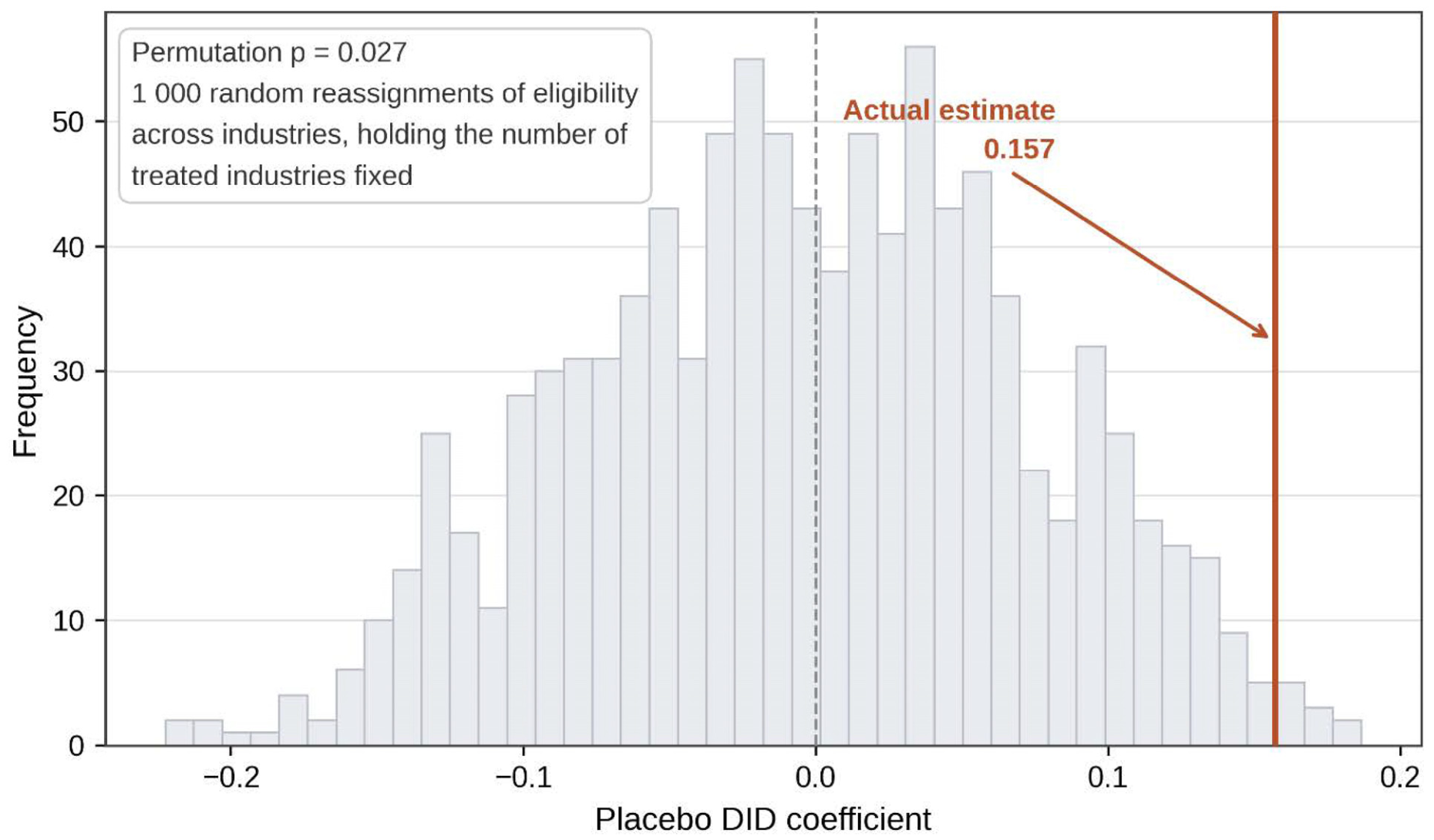
Figure 3 reports a randomization-inference test that reassigns industry eligibility across two-digit industries 1000 times, holding the number of treated industries fixed, and asks how often a placebo assignment produces an effect as large as the one we estimate. The actual estimate lies at the 97.6th percentile of that distribution (p = 0.027). A wild cluster bootstrap with the null imposed and Rademacher weights [47], 1999 replications clustered by industry, gives p = 0.009. An F-test for redundant fixed effects rejects the adequacy of pooled OLS, F(4050, 21,201) = 14.38, and a Hausman test rejects the consistency of random effects, χ²(7) = 21.63, p = 0.003, supporting the two-way fixed-effects specification.

Estimates by pilot sub-sector, which show the effect present in both advanced manufacturing and modern services, and further checks on alternative outcome transformations are omitted to save space and are available from the corresponding author on request.

6. Discussion and Conclusion

6.1. Summary of Findings

Using a two-way fixed-effects difference-in-differences design around China’s 2018 industry-targeted VAT credit refund pilot, we find an intention-to-treat effect of 0.172 without controls and 0.157 with a compact control vector, both significant at the 1 percent level (H1). The effect implies a 17.0 percent increase in green invention-patent applications. It survives removal of the control firms drawn in by the 2019 expansion, the addition of sector-by-year and province-by-year fixed effects, three heterogeneity-robust estimators, a propensity-score-matched sample, and randomization inference.

The mechanism evidence is consistent with the proposed pathway: the refund eases the SA financing-constraint index and raises R&D intensity, and the Monte Carlo-bounded indirect effect of the financing-to-R&D chain excludes zero (H2). This is a decomposition consistent with the hypothesized chain rather than identification of a sequential mechanism, since all three variables respond to the same shock within the same year.

The policy’s translation into innovation is conditioned by the firm’s structural governance and its external policy environment. Internal control quality significantly strengthens the conversion (H3). The effect concentrates among firms with greater pre-treatment financial slack and is absent in provinces with high CPU, where the refund raises neither cash holdings nor capital expenditure—an absent conversion rather than an identifiable alternative use.

6.2. Theoretical Implications

This study extends the tax-and-innovation literature beyond price-based instruments to a predominantly liquidity-based one, and in doing so exposes a gap in the theory that motivates most of that literature. Financing-constraints theory predicts that releasing a cash constraint raises investment in activities rationed by internal funds, but because cash is fungible, it cannot predict that the released funds reach any particular use. Our results locate the missing filter in two places: the firm’s structural control architecture, which determines whether an investment intention becomes monitored expenditure, and the credibility of the external policy environment, which determines whether an irreversible commitment is worth making at all. Fiscal liquidity is therefore better understood as a complement to governance quality and regulatory predictability than as a substitute for either, and models of policy transmission should treat the firm as an active filter rather than a passive conduit.

Why the effect concentrates where it does follows from the same logic. Green R&D is intangible, poorly collateralized and long-gestating, and it generates environmental benefits the firm cannot fully capture, all of which push it toward the back of the financing pecking order [23] whenever internal funds are the marginal source of finance. Ordinary capital expenditure, being tangible and verifiable ex ante, can draw on external debt even when cash is scarce. A liquidity injection that leaves relative prices unchanged should therefore be redirected disproportionately toward the investments most starved of internal funds, which is the pattern the baseline, mechanism and financial-slack results jointly document. Institutional quality complements the instrument rather than substituting for it because a liquidity injection lowers the financing hurdle for green R&D without raising the expected private return to holding a green patent or resolving uncertainty about the regulation the resulting technology will face. The same refund produces a 25.2 percent increase in green invention applications where climate policy is predictable and no measurable increase where it is not.

A methodological point also generalizes beyond this setting. When a policy’s proposed mechanism variable is itself a plausible mediator, including it as a control in the headline regression introduces bias rather than guarding against it. Excluding the SA index from the baseline control set while retaining it as the object of the mechanism test follows from this reasoning, as does forming every subsample split on pre-treatment rather than contemporaneous values.

Policy Implications

For governments designing environmental fiscal policy, the most immediate lesson is that liquidity-based instruments can complement price-based incentives at the higher-quality tier of green innovation. The triple-difference evidence shows the response concentrating in substantively examined invention applications rather than in unexamined utility models, so the refund is not simply purchasing filing volume. That said, because the effect concentrates in firms with greater financial slack and stronger internal controls, untargeted refunds may deliver limited environmental returns where those conditions bind, and pairing liquidity support with governance-aware targeting could raise the environmental return on a given fiscal outlay. The absence of any response where CPU is high carries a further implication: liquidity alone is not sufficient when the future direction of environmental regulation is unclear, so credible and well-communicated climate roadmaps are a necessary companion to fiscal support rather than an unrelated policy track.

These lessons are not specific to China. Uncredited input-VAT balances arise mechanically in any credit-invoice VAT system whenever firms make large, front-loaded purchases of capital goods or research inputs, and slow or restricted refunding is a well-documented feature of VAT administration across many emerging and developing economies. Accelerating VAT refunds can be implemented quickly, requires no new rates or credits, and reaches firms that price-based incentives systematically miss, among them young, loss-making, or capital-intensive firms with little taxable income against which to claim a deduction. Because refunded cash remains fungible, however, the environmental return is not automatic, and jurisdictions with weaker internal-control and disclosure regimes should expect a smaller green dividend from the same outlay.

Our sample covers listed firms, so these conclusions apply directly only to them, and the likely direction of external validity is not neutral. The effect concentrates among firms with greater financial slack, and unlisted small and medium enterprises are typically more constrained, so the marginal value of a refund may well be higher there; yet those same firms typically operate weaker internal control architecture, which our results identify as the structural condition for conversion. Since the two considerations pull in opposite directions, we would suggest extending refunds to unlisted firms with simplified claim procedures, given that administrative complexity deters small firms disproportionately and fewer than half of even listed eligible firms claimed, while calibrating expectations of the environmental return to the weaker control environment rather than extrapolating from listed-firm estimates. Evaluation using tax-administration microdata covering unlisted firms would resolve the question directly.

Because the mechanism we document runs from public fiscal design through corporate financing to green technological output, the findings speak to two Sustainable Development Goals in particular. Targets 9.4 and 9.5 call for upgrading industry toward clean technologies and enhancing technological capabilities, and our mechanism evidence shows the refund raising R&D intensity, while the baseline shows that input translates into green invention-patent applications. The boundary-condition results add a design lesson for this goal: liquidity relief upgrades industrial R&D capability most reliably where the firm has both the headroom and the control architecture to convert cash into a monitored research program. Target 13.2 calls for integrating climate measures into national planning, and our CPU result is in effect an empirical statement about what happens when that integration is incomplete. Because we measure invention rather than deployment, the contribution is upstream: the policy expands the stock of low-carbon technology available for later diffusion rather than reducing emissions directly.

6.3. Limitations and Conclusion

Several limitations temper these conclusions. Refund take-up within eligible industries was not exogenous, so defining treatment as industry eligibility yields an intention-to-treat effect diluted by non-claiming eligible firms; administrative refund records would sharpen identification. Financing constraints, R&D investment and innovation are plausibly jointly determined, so the decomposition is consistent with the proposed chain without establishing its temporal ordering. Patent applications measure inventive commitment rather than emissions reduced, and counts do not measure technological significance: the triple difference against utility models establishes that the response is on the examined margin, but cannot distinguish a marginal invention from a significant one, and citation-weighted counts, patent family size and originality indices would allow that distinction. Spillovers are a further limitation, since treated and control firms compete in input and technology markets and the direction of any spillover is not identified in our design. Finally, the CPU measure is a provincial aggregate merged to firms by registered province and year, which may mask city-level heterogeneity, and our attribution of the effect to a predominantly liquidity-based channel rests on the refund’s institutional design rather than on an instrument that mechanically rules out improved borrowing capacity or altered lender expectations.

Improving firms’ cash position through the tax system can promote high-quality green innovation, but conditionally, and on more dimensions than financing constraints alone. The VAT credit refund raises green invention-patent applications by 17.0 percent through a channel consistent with financing relief and R&D expansion, and the result is stable across every specification, estimator and placebo we test. Its efficacy hinges on conditions we can specify: it is stronger where internal controls are robust and financial slack is ample, and it is essentially absent where CPU is high. For governments turning to fiscal liquidity to pursue environmental goals, the instrument works, but selectively. Internal governance and external policy predictability jointly determine how much green innovation a given refund ultimately buys, and fiscal liquidity is, based on this evidence, a complement to institutional quality rather than a substitute for it.

References

1. Aghion, P.; Boneva, L.; Breckenfelder, J.; Laeven, L.A.; Olovsson, C.; Popov, A.A.; Rancoita, E. Financial Markets and Green Innovation. SSRN J. 2022. [Google Scholar] [CrossRef] [Scilit]
2. Ockwell, D.G.; Byrne, R. Sustainable Energy for All: Innovation, Technology and Pro-Poor Green Transformations; Pathways to Sustainability; Routledge, Taylor & Francis Group, Earthscan, from Routledge: London, UK; New York, NY, USA, 2017; ISBN 978-1-138-65692-5. [Google Scholar]
3. Zhao, S.; Li, W. Supply Chain ESG Spillovers and Firm Green Innovation: Evidence from China. Technol. Anal. Strateg. Manag. 2026, 1–19. [Google Scholar] [CrossRef] [Scilit]
4. Feng, Z.; Wijethilake, C. The Impact of Green Innovation and Green Finance on Corporate ESG Performance. Bus. Strat. Environ. 2026, bse.71050. [Google Scholar] [CrossRef] [Scilit]
5. Acemoglu, D.; Aghion, P.; Bursztyn, L.; Hemous, D. The Environment and Directed Technical Change. Am. Econ. Rev. 2012, 102, 131–166. [Google Scholar] [CrossRef] [Scilit] [PubMed]
6. Jaffe, A.B.; Newell, R.G.; Stavins, R.N. A Tale of Two Market Failures: Technology and Environmental Policy. Ecol. Econ. 2005, 54, 164–174. [Google Scholar] [CrossRef] [Scilit]
7. Bloom, N.; Griffith, R.; Van Reenen, J. Do R&D Tax Credits Work? Evidence from a Panel of Countries 1979–1997. J. Public Econ. 2002, 85, 1–31. [Google Scholar] [CrossRef] [Scilit]
8. Rao, N. Do Tax Credits Stimulate R&D Spending? The Effect of the R&D Tax Credit in Its First Decade. J. Public Econ. 2016, 140, 1–12. [Google Scholar] [CrossRef] [Scilit]
9. Zwick, E.; Mahon, J. Tax Policy and Heterogeneous Investment Behavior. Am. Econ. Rev. 2017, 107, 217–248. [Google Scholar] [CrossRef] [Scilit]
10. Liu, L.; Cao, L.; Cao, Y.; Lu, M.; Shan, Y. VAT Credit Refunds and Firm Productivity: Evidence from China’s VAT Reform. Int. Rev. Financ. Anal. 2024, 93, 103171. [Google Scholar] [CrossRef] [Scilit]
11. Yang, X.; Dong, X.; Zeng, Y. Rains after the Drought: The Impact of VAT Credit Refund on Corporate R&D Expenditures in China. Appl. Econ. 2025, 57, 6804–6819. [Google Scholar] [CrossRef] [Scilit]
12. Li, M.; Liu, C.; Yu, Z. Liquidity Shocks, Capital Allocation, and Corporate Environmental Rating: Evidence from Tax Refunds. Emerg. Mark. Financ. Trade 2026, 1–19. [Google Scholar] [CrossRef] [Scilit]
13. Brown, J.R.; Fazzari, S.M.; Petersen, B.C. Financing Innovation and Growth: Cash Flow, External Equity, and the 1990s R&D Boom. J. Financ. 2009, 64, 151–185. [Google Scholar] [CrossRef] [Scilit]
14. Hall, B.H.; Lerner, J. The Financing of R&D and Innovation. In Handbook of the Economics of Innovation; Elsevier: Amsterdam, The Netherlands, 2010; Volume 1, pp. 609–639. ISBN 978-0-444-51995-5. [Google Scholar]
15. Han, L.; Peng, Y.; Liu, F. The Effect of Tax Neutrality Reform on Cash Dividend Policy: Evidence from China’s Vat Credit Refund. Appl. Econ. 2025, 1–19. [Google Scholar] [CrossRef] [Scilit]
16. Xie, Y.; Qin, J.; Jin, Z.; Geng, M. VAT Neutrality and Corporate Cash Holdings —Based on the Research of Uncredited VAT Refund Policy. China Financ. Econ. Rev. 2023, 12, 49–71. [Google Scholar] [CrossRef] [Scilit]
17. DeAngelo, H.; Kahle, K.; Skinner, D.J. Agency Cost of Free Cash Flow, Capital Allocation, and Payouts. J. Financ. Econ. 2025, 172, 104117. [Google Scholar] [CrossRef] [Scilit]
18. Jensen, M.C. Agency Costs of Free Cash Flow, Corporate Finance, and Takeovers. Am. Econ. Rev. 1986, 76, 323–329. [Google Scholar]
19. Sun, L.; Abraham, S. Estimating Dynamic Treatment Effects in Event Studies with Heterogeneous Treatment Effects. J. Econom. 2021, 225, 175–199. [Google Scholar] [CrossRef] [Scilit]
20. Callaway, B.; Sant’Anna, P.H.C. Difference-in-Differences with Multiple Time Periods. J. Econom. 2021, 225, 200–230. [Google Scholar] [CrossRef] [Scilit]
21. Gardner, J. Two-Stage Differences in Differences. arXiv 2022, arXiv:2207.05943. [Google Scholar]
22. Fazzari, S.M.; Hubbard, R.G.; Petersen, B.C.; Blinder, A.S.; Poterba, J.M. Financing Constraints and Corporate Investment. Brook. Pap. Econ. Act. 1988, 1988, 141. [Google Scholar] [CrossRef] [Scilit]
23. Myers, S.C.; Majluf, N.S. Corporate Financing and Investment Decisions When Firms Have Information That Investors Do Not Have. J. Financ. Econ. 1984, 13, 187–221. [Google Scholar] [CrossRef] [Scilit]
24. Yue, T.; Tong, J.; Guo, Y.; Zhang, C. Short-Term Relief and Green Transformation: Evidence from the Unintended Environmental Governance Effects of China’s VAT Credit Refund Policy. Econ. Anal. Policy 2025, 86, 1725–1747. [Google Scholar] [CrossRef] [Scilit]
25. Hubbard, R.G. Capital-Market Imperfections and Investment. J. Econ. Lit. 1998, 36, 193–225. [Google Scholar]
26. Stiglitz, J.E.; Weiss, A. Credit Rationing in Markets with Imperfect Information. Am. Econ. Rev. 1981, 71, 393–410. [Google Scholar]
27. Li, J.; Ge, L.; Zeng, L. Tax Incentive and Corporate Hiring Decisions: Evidence from China’s VAT Credit Refund Policy. Manag. Decis. Econ. 2024, 45, 414–427. [Google Scholar] [CrossRef] [Scilit]
28. Zhao, Z.; Yue, Y.; Wang, W. Unintended Consequences of Tax Incentives on Firms’ Human Capital Composition: Evidence from China. China Econ. Rev. 2024, 84, 102138. [Google Scholar] [CrossRef] [Scilit]
29. Zhu, L.; Zhou, T.; Wen, Y. Tax Incentive and Stock Price Crash Risk: Evidence from VAT Credit Refund Policy of China. Res. Int. Bus. Financ. 2025, 78, 102974. [Google Scholar] [CrossRef] [Scilit]
30. Mao, Q.; Wang, Y. VAT Credit Refund Policy and Outward Foreign Direct Investment: Firm-level Evidence from China. Contemp. Econ. Policy 2026, 44, 717–735. [Google Scholar] [CrossRef] [Scilit]
31. Bai, D.; Du, L.; Xu, Y.; Abbas, S. Climate Policy Uncertainty and Corporate Green Innovation: Evidence from Chinese A-Share Listed Industrial Corporations. Energy Econ. 2023, 127, 107020. [Google Scholar] [CrossRef] [Scilit]
32. Hadlock, C.J.; Pierce, J.R. New Evidence on Measuring Financial Constraints: Moving Beyond the KZ Index. Rev. Financ. Stud. 2010, 23, 1909–1940. [Google Scholar] [CrossRef] [Scilit]
33. Chen, H.; Dong, W.; Han, H.; Zhou, N. A Comprehensive and Quantitative Internal Control Index: Construction, Validation, and Impact. Rev. Quant. Financ. Account. 2017, 49, 337–377. [Google Scholar] [CrossRef] [Scilit]
34. Bloom, N. The Impact of Uncertainty Shocks. Econometrica 2009, 77, 623–685. [Google Scholar] [CrossRef] [Scilit]
35. Dixit, R.K.; Pindyck, R.S. Investment Under Uncertainty; Princeton University Press: Princeton, NJ, USA, 1994; ISBN 978-1-4008-3017-6. [Google Scholar]
36. Ma, Y.-R.; Liu, Z.; Ma, D.; Zhai, P.; Guo, K.; Zhang, D.; Ji, Q. A News-Based Climate Policy Uncertainty Index for China. Sci. Data 2023, 10, 881. [Google Scholar] [CrossRef] [Scilit] [PubMed]
37. Wang, M.; Wurgler, J.; Zhang, H. Policy Uncertainty Reduces Green Innovation. J. Financ. Econ. 2026, 175, 104189. [Google Scholar] [CrossRef] [Scilit]
38. Blanchard, O.J.; Lopez-de-Silanes, F.; Shleifer, A. What Do Firms Do with Cash Windfalls? J. Financ. Econ. 1994, 36, 337–360. [Google Scholar] [CrossRef] [Scilit]
39. Qi, B.; Li, L.; Zhou, Q.; Sun, J. Does Internal Control over Financial Reporting Really Alleviate Agency Conflicts? Account. Financ. 2017, 57, 1101–1125. [Google Scholar] [CrossRef] [Scilit]
40. Ahmad, S.; Akbar, S.; Halari, A.; Shah, S.Z. Organizational Non-Compliance with Principles-Based Governance Provisions and Corporate Risk-Taking. Int. Rev. Financ. Anal. 2021, 78, 101884. [Google Scholar] [CrossRef] [Scilit]
41. Denis, D.J.; Sibilkov, V. Financial Constraints, Investment, and the Value of Cash Holdings. Rev. Financ. Stud. 2010, 23, 247–269. [Google Scholar] [CrossRef] [Scilit]
42. Cheng, Z.; Wu, Y. The Impact of Climate Policy Uncertainty on Corporate ESG Greenwashing. J. Environ. Manag. 2025, 394, 127353. [Google Scholar] [CrossRef] [Scilit] [PubMed]
43. Preacher, K.J.; Selig, J.P. Advantages of Monte Carlo Confidence Intervals for Indirect Effects. Commun. Methods Meas. 2012, 6, 77–98. [Google Scholar] [CrossRef] [Scilit]
44. Qian, B.; Tan, Y.; Power, G.; Mandal, A. Economic Policy Uncertainty, Information Production, and Transparency. Int. Rev. Financ. Anal. 2025, 103, 104203. [Google Scholar] [CrossRef] [Scilit]
45. Dechezleprêtre, A.; Einiö, E.; Martin, R.; Nguyen, K.-T.; Van Reenen, J. Do Tax Incentives Increase Firm Innovation? An RD Design for R&D, Patents, and Spillovers. Am. Econ. J. Econ. Policy 2023, 15, 486–521. [Google Scholar] [CrossRef] [Scilit]
46. Caliendo, M.; Kopeinig, S. Some Practical Guidance for the Implementation of Propensity Score Matching. J. Econ. Surv. 2008, 22, 31–72. [Google Scholar] [CrossRef] [Scilit]
47. Cameron, A.C.; Gelbach, J.B.; Miller, D.L. Bootstrap-Based Improvements for Inference with Clustered Errors. Rev. Econ. Stat. 2008, 90, 414–427. [Google Scholar] [CrossRef] [Scilit]
Figure 1. Conceptual framework. The VAT credit refund improves firm liquidity, easing financing constraints and raising R&D investment intensity, which in turn raises green invention-patent applications (H1, H2). Internal control quality conditions this conversion (H3). Pre-treatment financial slack and provincial CPU further condition the magnitude of the response.
Sustainability 18 08409 g001
Figure 2. Event-study estimates and pre-trend analysis. Estimated year-specific treatment effects from the event-study specification, using 2017 as the omitted reference year. Error bars denote 95 percent confidence intervals from industry-clustered standard errors. The horizontal dashed line indicates a zero treatment effect, and the dotted vertical line marks the June-2018 pilot. Firm and year fixed effects and the baseline control vector are included.
Sustainability 18 08409 g002
Figure 3. Randomization inference. Distribution of the DID coefficient when industry eligibility is randomly reassigned across two-digit industries, holding the number of treated industries fixed. The vertical solid line indicates the actual DID coefficient estimate, while the vertical dashed line marks the null value of zero.
Sustainability 18 08409 g003