Author Contributions
Conceptualization, A.H. and A.M.K.; methodology, A.H., A.M.K. and M.J.A.; software, A.M.K.; validation, M.J.A. and D.T.; formal analysis, A.H. and A.M.K.; investigation, F.T.A.-O. and A.O.S.A.; data curation, A.M.K. and F.T.A.-O.; writing—original draft, A.H. and A.M.K.; writing—review and editing, M.J.A., D.T., F.T.A.-O. and A.O.S.A.; visualisation, A.M.K.; supervision, A.H.; project administration, A.H.; funding acquisition, A.H. All authors have read and agreed to the published version of the manuscript.
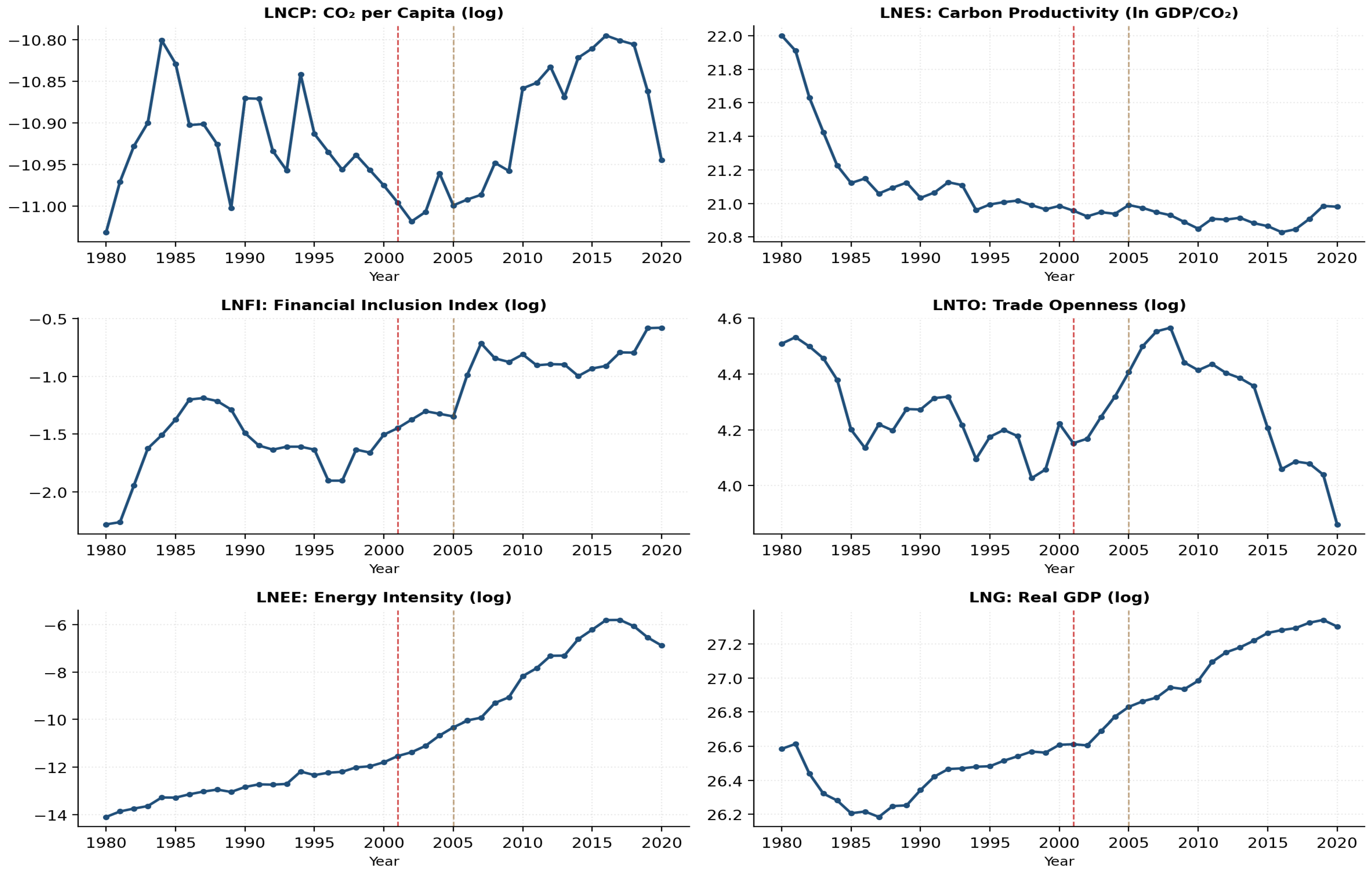
Figure 1.
Time-series plots of LNCP, LNES, LNFI, LNTO, LNEE, and LNG, 1980–2020. Vertical lines mark the 2001 Chow-test break date (red dashed) and the 2005 WTO accession (gold dashed). The structural shift around 2001–2005 is evident in LNFI (a clear step-up after 2005), LNEE (acceleration of the long-run trend), and LNTO (a regime change).
Figure 1.
Time-series plots of LNCP, LNES, LNFI, LNTO, LNEE, and LNG, 1980–2020. Vertical lines mark the 2001 Chow-test break date (red dashed) and the 2005 WTO accession (gold dashed). The structural shift around 2001–2005 is evident in LNFI (a clear step-up after 2005), LNEE (acceleration of the long-run trend), and LNTO (a regime change).
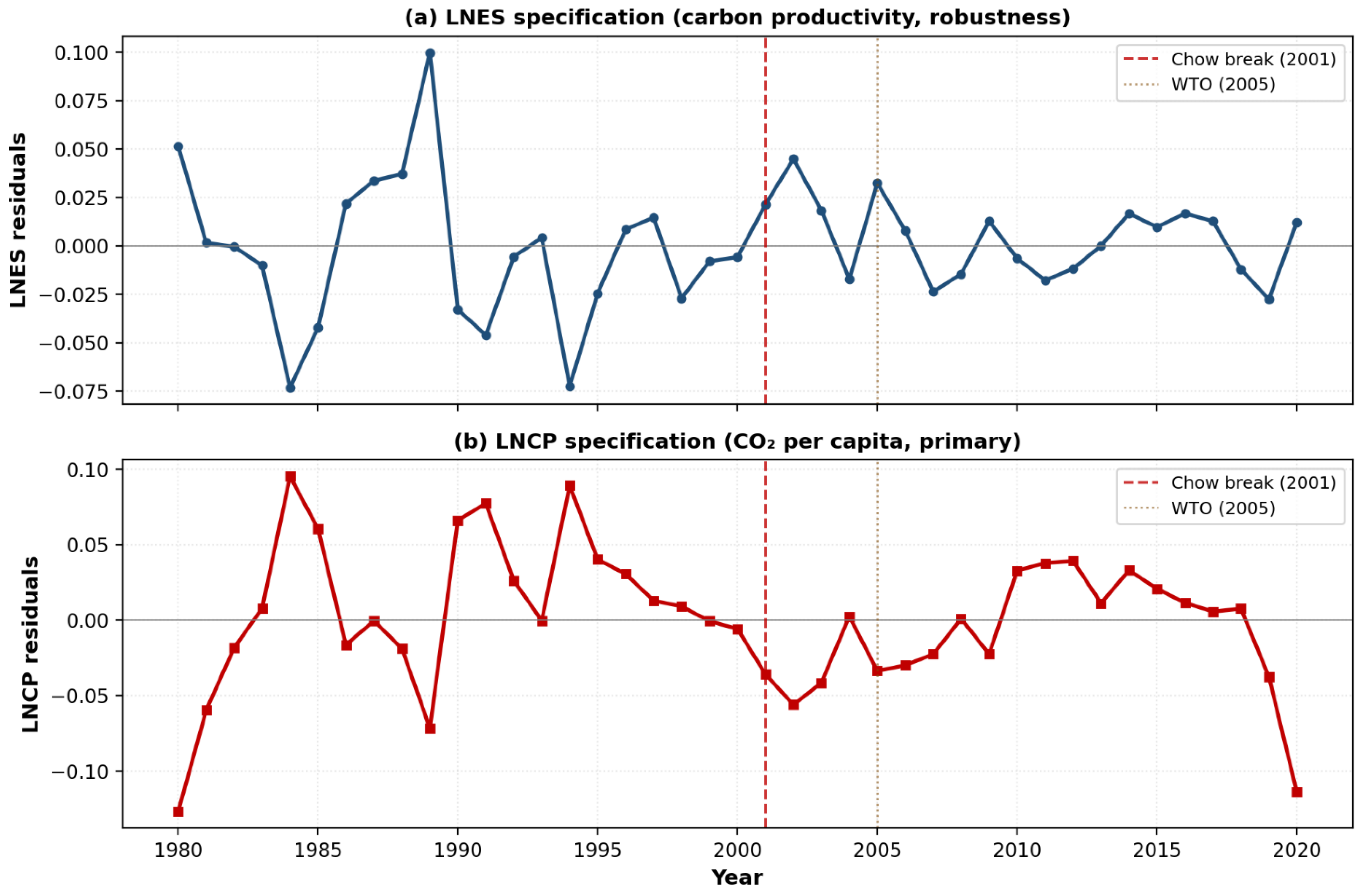
Figure 2.
Cointegrating residuals from the LNES specification (panel (
a)) and the primary LNCP specification (panel (
b)). The LNCP residuals show much greater pre-2001 volatility and stabilise after the 2001 break, consistent with the Chow and Bai–Perron sup-F evidence in
Table 8. Red dashed line: 2001 Chow-test primary break. Gold dotted line: 2005 WTO accession (policy robustness).
Figure 2.
Cointegrating residuals from the LNES specification (panel (
a)) and the primary LNCP specification (panel (
b)). The LNCP residuals show much greater pre-2001 volatility and stabilise after the 2001 break, consistent with the Chow and Bai–Perron sup-F evidence in
Table 8. Red dashed line: 2001 Chow-test primary break. Gold dotted line: 2005 WTO accession (policy robustness).
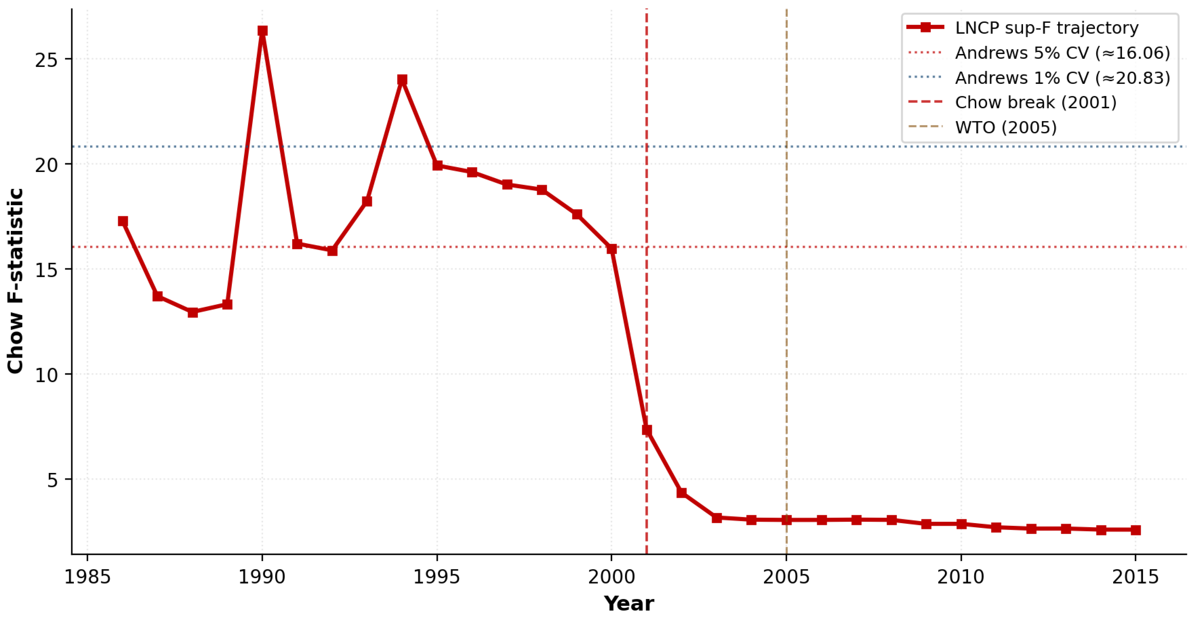
Figure 3.
Bai–Perron sup-F trajectory: Chow F-statistic computed at each candidate break year over the trimmed sample range. The LNCP trajectory exceeds the 5% Andrews critical value (16.06) for multiple early-1990s candidates and attains its highest value in 1990 (sup-F = 26.37). After 2001, the F-statistic collapses below the critical value, confirming structural stability post-2001.
Figure 3.
Bai–Perron sup-F trajectory: Chow F-statistic computed at each candidate break year over the trimmed sample range. The LNCP trajectory exceeds the 5% Andrews critical value (16.06) for multiple early-1990s candidates and attains its highest value in 1990 (sup-F = 26.37). After 2001, the F-statistic collapses below the critical value, confirming structural stability post-2001.
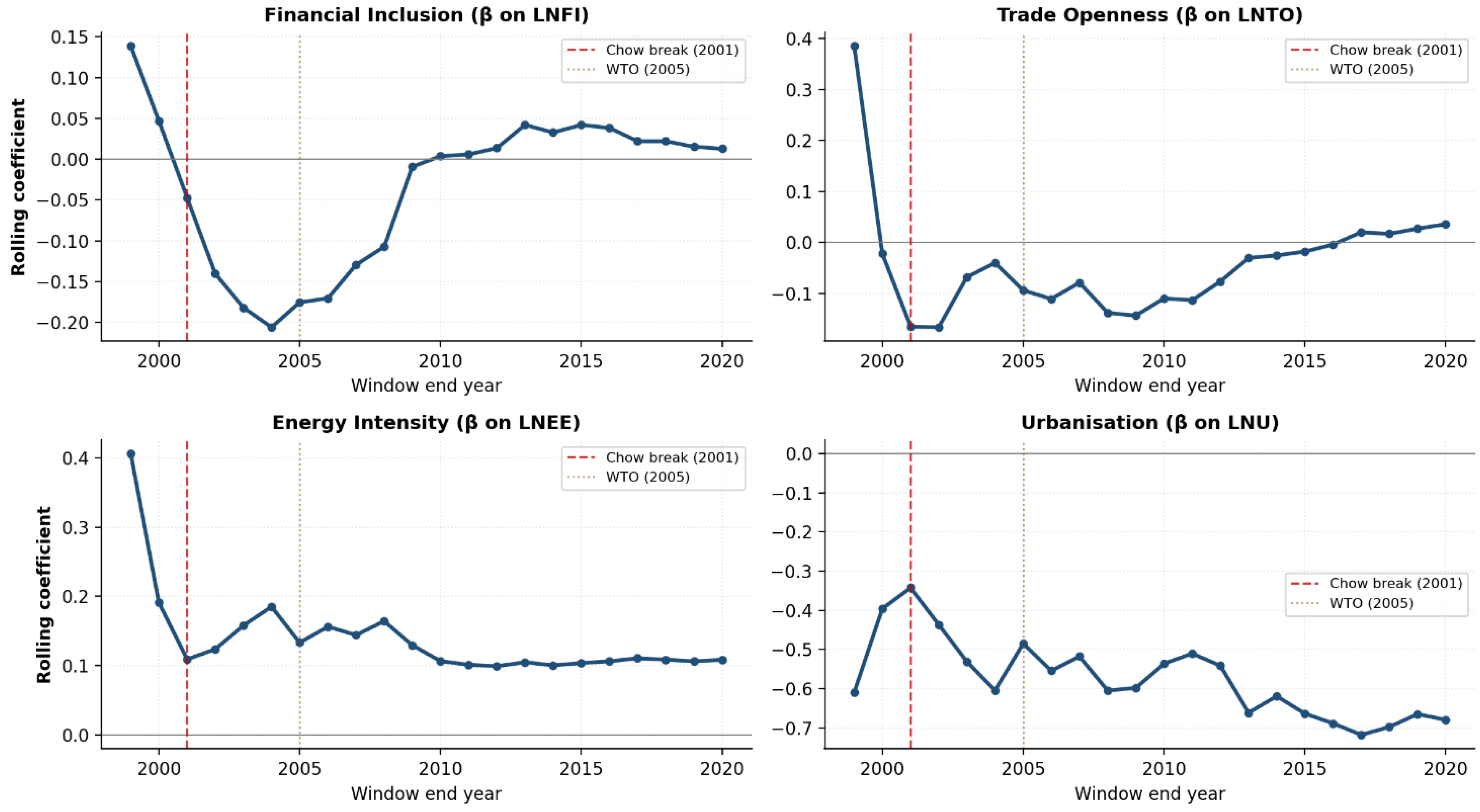
Figure 4.
Rolling-window OLS coefficients (20-year window) for the primary LNCP specification. Each panel shows how the coefficient on the corresponding driver evolves as the estimation window slides through the sample. The financial-inclusion coefficient stabilises near zero after the 2001 break; energy intensity converges to a stable positive coefficient (≈0.11) post-2001; trade openness rises through the post-WTO period; urbanisation becomes more strongly negative. Red dashed line: 2001 Chow-test primary break. Gold dotted line: 2005 WTO accession.
Figure 4.
Rolling-window OLS coefficients (20-year window) for the primary LNCP specification. Each panel shows how the coefficient on the corresponding driver evolves as the estimation window slides through the sample. The financial-inclusion coefficient stabilises near zero after the 2001 break; energy intensity converges to a stable positive coefficient (≈0.11) post-2001; trade openness rises through the post-WTO period; urbanisation becomes more strongly negative. Red dashed line: 2001 Chow-test primary break. Gold dotted line: 2005 WTO accession.
Figure 5.
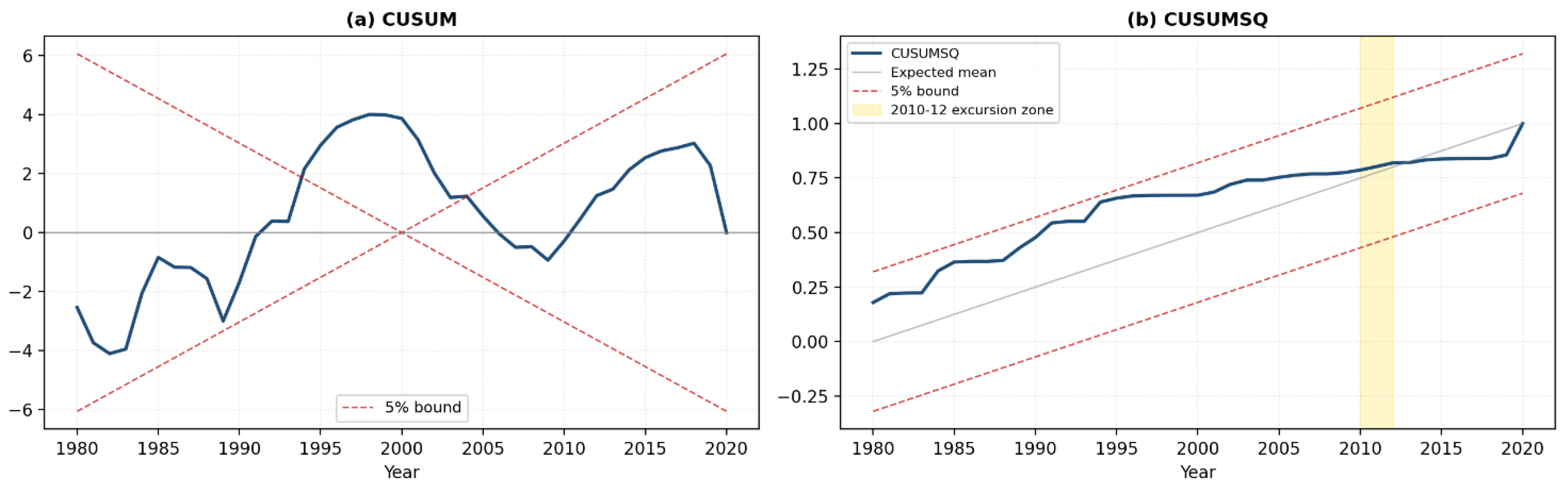
(a) CUSUM plot of recursive residuals (primary LNCP ARDL specification): the statistic remains within the 5% significance bounds throughout the effective sample period. (b) CUSUMSQ plot: the statistic tracks the expected mean line but briefly approaches the upper bound around 2010–2012 (shaded region), coinciding with the post-2009 oil-price recovery, the Arab Spring (from December 2010), and the 2011 Saudi domestic stimulus package. In both panels, the blue line denotes the test statistic (CUSUM in panel (a), CUSUMSQ in panel (b)), the grey line denotes the expected mean, and the red dashed lines denote the 5% significance bounds.
Figure 5.
(a) CUSUM plot of recursive residuals (primary LNCP ARDL specification): the statistic remains within the 5% significance bounds throughout the effective sample period. (b) CUSUMSQ plot: the statistic tracks the expected mean line but briefly approaches the upper bound around 2010–2012 (shaded region), coinciding with the post-2009 oil-price recovery, the Arab Spring (from December 2010), and the 2011 Saudi domestic stimulus package. In both panels, the blue line denotes the test statistic (CUSUM in panel (a), CUSUMSQ in panel (b)), the grey line denotes the expected mean, and the red dashed lines denote the 5% significance bounds.
Table 1.
Variable definitions and data sources.
Table 1.
Variable definitions and data sources.
| Variable | Symbol | Definition | Source | Expected Sign |
|---|
| CO2 per capita | LNCP | ln of total CO2 emissions/population (primary dependent variable) | WDI | Dependent |
| Carbon productivity | LNES | ln of real GDP/CO2 emissions (robustness) | WDI | Alt. dependent |
| Financial inclusion | LNFI | ln of Financial Institutions Access Index | IMF FAS | ±(regime-dependent) |
| Trade openness | LNTO | ln of (exports + imports)/GDP | WDI | ± |
| Energy intensity | LNEE | ln of energy use per unit of real GDP (lower = higher efficiency) | WDI | +on LNCP (higher intensity → higher emissions) |
| Urbanisation | LNU | ln of urban population share (% of total) | WDI | ± |
| Economic growth (LNES spec. only) | LNG | ln of real GDP (constant USD); not used in primary LNCP specification | WDI | +/−(EKC; LNES only) |
Table 2.
Descriptive statistics and Jarque–Bera normality tests (1980–2020; n = 41).
Table 2.
Descriptive statistics and Jarque–Bera normality tests (1980–2020; n = 41).
| Variable | Mean | Std. Dev. | Min | Max | Skewness | Kurtosis | JB p-Value |
|---|
| LNCP | −10.914 | 0.069 | −11.031 | −10.795 | 0.210 | −1.148 | 0.278 |
| LNES | 21.058 | 0.255 | 20.829 | 22.001 | 2.579 | 6.787 | <0.001 |
| LNFI | −1.302 | 0.435 | −2.283 | −0.578 | −0.304 | −0.493 | 0.562 |
| LNTO | 4.272 | 0.169 | 3.861 | 4.565 | −0.088 | −0.589 | 0.671 |
| LNEE | −10.674 | 2.689 | −14.103 | −5.794 | 0.622 | −1.087 | 0.104 |
| LNU | 16.330 | 0.567 | 15.198 | 17.096 | −0.367 | −0.995 | 0.268 |
| LNG | 26.717 | 0.367 | 26.185 | 27.342 | 0.362 | −1.147 | 0.211 |
Table 3.
Pearson correlation matrix and variance inflation factors.
Table 3.
Pearson correlation matrix and variance inflation factors.
| | LNCP | LNES | LNFI | LNTO | LNEE | LNU | LNG |
|---|
| LNCP | 1.000 | −0.305 | 0.383 | −0.218 | 0.479 | 0.254 | 0.333 |
| LNES | −0.305 | 1.000 | −0.698 | 0.396 | −0.611 | −0.791 | −0.429 |
| LNFI | 0.383 | −0.698 | 1.000 | −0.146 | 0.819 | 0.795 | 0.687 |
| LNTO | −0.218 | 0.396 | −0.146 | 1.000 | −0.191 | −0.244 | −0.081 |
| LNEE | 0.479 | −0.611 | 0.819 | −0.191 | 1.000 | 0.925 | 0.957 |
| LNU | 0.254 | −0.791 | 0.795 | −0.244 | 0.925 | 1.000 | 0.879 |
| LNG | 0.333 | −0.429 | 0.687 | −0.081 | 0.957 | 0.879 | 1.000 |
| VIF (LNES spec.) | — | — | 5.30 | 1.38 | 38.28 | 7.58 | 23.09 |
| VIF (LNCP spec.) | — | — | 3.41 | 1.07 | 8.18 | 7.86 | — |
Table 4.
Unit root tests: ADF, Phillips–Perron, and Zivot–Andrews (one endogenous break, Model C).
Table 4.
Unit root tests: ADF, Phillips–Perron, and Zivot–Andrews (one endogenous break, Model C).
| Variable | ADF (Level) | ADF (Δ) | PP (Level) | PP (Δ) | Z–A t-Stat (Level) | Z–A Break Year | Order |
|---|
| LNCP | −2.163 | −3.479 *** | −2.184 | −3.523 *** | −4.190 | 2010 | I(1) |
| LNES | −1.791 | −5.066 *** | −1.853 | −5.183 *** | −7.580 *** | 2015 | I(0) w/break |
| LNFI | −1.667 | −4.523 *** | −1.781 | −4.498 *** | −4.567 | 2000 | I(1) |
| LNTO | −1.627 | −4.184 *** | −1.210 | −4.252 *** | −3.168 | 2005 | I(1) |
| LNEE | −1.283 | −3.264 ** | −0.210 | −3.880 *** | −3.238 | 1995 | I(1) |
| LNU | −1.787 | −3.142 ** | −1.622 | −3.087 ** | −3.577 | 2015 | I(1) |
| LNG | −0.067 | −3.639 *** | 0.262 | −3.660 *** | −7.233 *** | 2011 | I(0) w/break |
Table 5.
ARDL bounds test for cointegration.
Table 5.
ARDL bounds test for cointegration.
| Specification | F-Statistic | t-Statistic (ECT) | 5% Bounds (k as Shown) |
|---|
| LNCP (primary, k = 4) | 4.050 | −4.820 | F: 2.86/3.49; t: −2.86/−3.99 |
| LNES (robustness, k = 5) | 4.500 | −5.600 | F: 2.62/3.79; t: −2.86/−4.19 |
Table 6.
ARDL long-run and short-run estimates (primary specification: dependent variable LNCP).
Table 6.
ARDL long-run and short-run estimates (primary specification: dependent variable LNCP).
| Variable | Coefficient | Std. Error | p-Value |
|---|
| Long run | | | |
| LNFI | 0.013 | 0.030 | 0.665 |
| LNTO | 0.022 | 0.024 | 0.358 |
| LNEE | 0.092 *** | 0.010 | 0.000 |
| LNU | −0.412 *** | 0.108 | 0.001 |
| Short run | | | |
| ΔLNFI | 0.008 | 0.024 | 0.731 |
| ΔLNTO | −0.094 * | 0.049 | 0.064 |
| ΔLNTO (−1) | 0.123 *** | 0.038 | 0.003 |
| ΔLNEE | 0.103 *** | 0.014 | 0.000 |
| ΔLNU | −0.831 *** | 0.241 | 0.002 |
| ECT (−1) | −0.610 *** | 0.116 | 0.000 |
| R2 | 0.872 | — | — |
| Adjusted R2 | 0.823 | — | — |
| F-statistic | 17.8 *** | — | 0.000 |
| Durbin–Watson | 2.04 | — | — |
Table 7.
Robustness check using FMOLS, DOLS, and CCR (primary specification, dep. variable: LNCP).
Table 7.
Robustness check using FMOLS, DOLS, and CCR (primary specification, dep. variable: LNCP).
| Variable | FMOLS Coef. | FMOLS P | DOLS Coef. | DOLS P | CCR Coef. | CCR P |
|---|
| LNFI | 0.018 | 0.490 | 0.012 | 0.701 | 0.020 | 0.451 |
| LNTO | 0.027 | 0.241 | 0.031 | 0.213 | 0.028 | 0.228 |
| LNEE | 0.093 *** | 0.000 | 0.078 *** | 0.002 | 0.094 *** | 0.000 |
| LNU | −0.418 *** | 0.000 | −0.402 *** | 0.000 | −0.420 *** | 0.000 |
| Constant | −4.110 | 0.001 | −3.890 | 0.002 | −4.130 | 0.001 |
Table 8.
Structural break test battery (primary specification, LNCP).
Table 8.
Structural break test battery (primary specification, LNCP).
| Test | Statistic | Break Year | Conclusion |
|---|
| Bai–Perron sup-F | F = 26.37 | 1990 | Significantly above 1% Andrews CV (≈20.8); confirms a major break in the early 1990s |
| Chow in 1986 (oil-price collapse) | F = 17.29 *** | 1986 | Significant at 1% |
| Chow in 1995 | F = 19.92 *** | 1995 | Significant at 1% |
| Chow at 2001 (close to Z–A breaks for LNFI/LNTO) | F = 7.36 *** | 2001 | Significant at 1%; primary break date for sub-sample re-estimation |
| Chow in 2005 (WTO accession) | F = 3.04 ** | 2005 | Significant at 5% (policy robustness check) |
| Chow in 2010 | F = 2.85 ** | 2010 | Significant at 5%; coincides with CUSUMSQ excursion (Section 4.7) |
Table 9.
Sub-sample re-estimation around the 2001 (primary) and 2005 (policy robustness) break dates.
Table 9.
Sub-sample re-estimation around the 2001 (primary) and 2005 (policy robustness) break dates.
| Variable | LNCP Pre-2001 (n = 21) | LNCP Post-2001 (n = 20) | LNCP Pre-WTO 2005 (n = 25) | LNCP Post-WTO 2005 (n = 16) |
|---|
| LNFI | 0.088 (p = 0.249) | 0.013 (p = 0.665) | 0.047 (p = 0.474) | 0.033 *** (p = 0.007) |
| LNTO | 0.050 (p = 0.893) | 0.036 (p = 0.018) ** | −0.197 (p = 0.188) | 0.054 (p = 0.004) * |
| LNEE | 0.224 (p = 0.313) | 0.108 (p < 0.001) * | 0.021 (p = 0.783) | 0.111 (p < 0.001) * |
| LNU | −0.415 (p = 0.159) | −0.680 (p < 0.001) * | −0.148 (p = 0.427) | −0.679 (p < 0.001) * |
| Constant | −1.529 (p = 0.814) | 1.302 (p = 0.470) | −7.398 (p = 0.088) | 1.234 (p = 0.251) |
| R2 | 0.389 | 0.985 | 0.292 | 0.996 |
| Adjusted R2 | 0.236 | 0.981 | 0.150 | 0.994 |
Table 10.
GDP-augmented post-2001 LNCP specification (n = 20). OLS standard errors are heteroscedasticity-robust (HC3); ridge coefficients use leave-one-out cross-validation (optimal penalty α = 0.001 on standardised data). R2 = 0.985. ** and *** denote significance at the 5% and 1% levels. The insignificant LNG coefficient and the stability of the other coefficients indicate that omitting GDP does not materially bias the estimates.
Table 10.
GDP-augmented post-2001 LNCP specification (n = 20). OLS standard errors are heteroscedasticity-robust (HC3); ridge coefficients use leave-one-out cross-validation (optimal penalty α = 0.001 on standardised data). R2 = 0.985. ** and *** denote significance at the 5% and 1% levels. The insignificant LNG coefficient and the stability of the other coefficients indicate that omitting GDP does not materially bias the estimates.
| Variable | OLS Coef. | OLS p-Value | Ridge Coef. |
|---|
| LNFI | 0.013 | 0.695 | 0.012 |
| LNTO | 0.036 | 0.025 ** | 0.036 |
| LNEE | 0.108 | <0.001 *** | 0.108 |
| LNU | −0.692 | <0.001 *** | −0.688 |
| LNG | 0.015 | 0.859 | 0.015 |
| Constant | 1.083 | 0.711 | — |
Table 11.
Break-date sensitivity: post-break long-run LNCP regression (LNFI, LNTO, LNEE, LNU) re-estimated at five candidate start years. Standard errors are heteroscedasticity-robust (HC3). ** and *** denote significance at the 5% and 1% levels. Energy intensity and urbanisation are significant at the 1% level for every candidate break; the substantive conclusions do not depend on the discretionary choice of 2001.
Table 11.
Break-date sensitivity: post-break long-run LNCP regression (LNFI, LNTO, LNEE, LNU) re-estimated at five candidate start years. Standard errors are heteroscedasticity-robust (HC3). ** and *** denote significance at the 5% and 1% levels. Energy intensity and urbanisation are significant at the 1% level for every candidate break; the substantive conclusions do not depend on the discretionary choice of 2001.
| Post-Break Start | n | R2 | LNFI | LNTO | LNEE | LNU |
|---|
| 1990 | 31 | 0.929 | −0.034 | 0.017 | 0.090 *** | −0.471 *** |
| 1995 | 26 | 0.979 | 0.013 | 0.026 | 0.104 *** | −0.645 *** |
| 2001 (primary) | 20 | 0.985 | 0.013 | 0.036 ** | 0.108 *** | −0.680 *** |
| 2005 (WTO) | 16 | 0.996 | 0.033 *** | 0.054 *** | 0.111 *** | −0.679 *** |
| 2010 | 11 | 0.993 | 0.005 | 0.004 | 0.115 *** | −0.774 *** |
Table 12.
Diagnostic and stability tests (primary LNCP ARDL specification).
Table 12.
Diagnostic and stability tests (primary LNCP ARDL specification).
| Diagnostic Test | Test Statistic | p-Value | Inference |
|---|
| Breusch–Godfrey LM (lags = 2) | 0.310 | 0.736 | No serial correlation |
| Breusch–Pagan–Godfrey | 2.140 | 0.084 | No significant heteroscedasticity |
| Jarque–Bera | 1.280 | 0.528 | Approximately normal |
| Ramsey RESET (squared fitted) | 1.620 | 0.214 | Correct functional form |
| CUSUM | Figure 5a | — | Within 5% bounds |
| CUSUMSQ | Figure 5b | — | Brief 2010–2012 excursion (see Section 4.7) |
Table 13.
Granger and Toda–Yamamoto causality tests.
Table 13.
Granger and Toda–Yamamoto causality tests.
| Null Hypothesis | Granger F (Lag 1) | Granger p | Toda–Yamamoto F | T–Y p |
|---|
| LNFI does not cause LNCP | 0.188 | 0.668 | 2.077 | 0.159 |
| LNCP does not cause LNFI | 0.345 | 0.561 | 0.044 | 0.836 |
| LNEE does not cause LNCP | 0.084 | 0.774 | 0.923 | 0.343 |
| LNCP does not cause LNEE | 6.338 ** | 0.017 | 0.000 | 0.993 |
| LNTO does not cause LNCP | 0.084 | 0.773 | 0.800 | 0.377 |
| LNCP does not cause LNTO | 0.031 | 0.862 | 0.806 | 0.376 |
| LNG does not cause LNCP | 2.982 * | 0.093 | 0.455 | 0.505 |
| LNCP does not cause LNG | 0.623 | 0.436 | 3.841 * | 0.058 |
| LNU does not cause LNCP | 1.749 | 0.195 | 8.166 *** | 0.007 |
| LNCP does not cause LNU | 0.310 | 0.581 | 0.112 | 0.740 |



 ,
,