Household Electricity Affordability Under Rising Costs in Vietnam: A Service–Capacity Gap Approach

Abstract

This study develops a Service–Capacity Gap (SCG) approach to examine household electricity affordability under rising costs in Vietnam. SCG compares each household’s electricity service-cost position with its core consumption-capacity position. Using 46,375 household-year observations from VHLSS 2012–2020, the study identifies four affordability positions: service-cost pressure (SCP: 36.60%), low service-cost non-pressure (LNP: 24.46%), capacity-supported service-cost (CSS: 20.73%), and low service-cost but capacity-constrained households (LCC: 18.21%). Benchmark comparisons show that high-burden and LIHC-type diagnostics align mainly with SCP, while low-use indicators split between LNP and LCC. LNP records only 2.22% LIHC-type risk despite 49.15% falling below the low-use threshold, whereas CSS exhibits no LIHC-type risk despite relatively high electricity costs. Socioeconomic profiles further show that LCC is more capacity-constrained than LNP, and CSS has stronger capacity than SCP. Under a 30% electricity-cost shock, new exposure reaches 28.99% for CSS and 19.03% for LNP. The main diagnostic value of SCG is that it resolves two ambiguities that conventional indicators tend to conflate: low service-cost can mean either non-pressure or hidden capacity constraint, while high service-cost can mean either affordability pressure or capacity-supported service use. Policy should use SCG to target low-use households with weak capacity (LCC), avoid automatic subsidies for low-use non-pressure households (LNP), and monitor near-boundary households exposed to rising costs.

1. Introduction

When household electricity access has reached a very high level, the welfare problem no longer lies only in whether households are connected to electricity. It lies in whether they can sustain electricity services without weakening their capacity to finance food, housing, education, and other core needs. This shift is consistent with the distinction between nominal connection and broader energy access [1], and with the SDG 7 focus on affordable, reliable, sustainable, and modern energy services rather than connection alone [2]. In this post-access setting, electricity affordability cannot be read only from bill size or expenditure share. Low electricity spending may reflect efficiency or genuinely low demand, but it may also reflect self-restriction. The key measurement problem is therefore to distinguish low spending that indicates affordability security from low spending that conceals restricted service under weak household capacity.

Existing measures capture important parts of this problem, but not the full service–capacity relationship. The burden-ratio and fuel-poverty tradition identifies visible pressure by comparing energy payments with household resources, as exemplified by the fuel-poverty approach [3] and the low-income-high-cost framework [4]. Later indicator studies refine this logic through alternative burden thresholds and indicator families. Evidence shows that energy-poverty indicators can identify different households depending on whether they emphasize expenditure, income, deprivation, or low resources [5,6]. These measures are useful for detecting high-payment pressure, but they are less informative when hardship appears as low electricity expenditure or when high expenditure is supported by stronger household capacity.

Low-use, minimum-use, and energy-service approaches address this limitation from a different angle. Energy-service approaches treat energy as an input into household functions and services [7,8], while benchmark-based approaches compare observed energy use with an equity-relevant standard to reveal hidden deprivation [9]. Hidden energy poverty has been linked to self-restriction in household energy use [10], while affordability ratios may overlook underconsumption of electricity and water services among lower-income households [11]. These approaches are complementary to burden measures, but they can still give conflicting signals. High bills may reflect hardship or capacity-supported service use, whereas low bills may reflect either low need or constrained consumption. What remains missing is a diagnostic framework that reads electricity service-cost position and household consumption capacity on the same comparative scale and separates these ambiguous low-cost and high-cost cases into policy-interpretable positions.

This gap is particularly relevant for Vietnam. Electricity access is now nearly universal, but household electricity use, appliance ownership, and electricity payments remain uneven across income groups and locations. Evidence from Vietnam shows that reductions in electricity poverty can coexist with rising energy-cost poverty [12], while objective improvements in electricity conditions do not necessarily translate into higher subjective satisfaction [13]. These findings reinforce the need to distinguish observed electricity conditions from welfare interpretation. Recent VHLSS-based evidence also shows that electricity-consumption differences across income groups have persisted and widened in the upper part of the distribution by 2020 [14,15]. After access expansion, the question is which households face a mismatch between electricity service cost and consumption capacity, which households are close to that boundary, and which households may become vulnerable when electricity costs rise. Vietnam provides a post-access setting in which the added value of a service–capacity diagnostic can be assessed empirically rather than only proposed conceptually.

This study develops a Service–Capacity Gap (SCG) approach to address that problem. SCG compares two relative household positions within each survey year: electricity service-cost position and core consumption-capacity position. A positive SCG indicates service–capacity pressure, while a non-positive SCG indicates capacity support. Using VHLSS 2012–2020 data, the study constructs the two positions, classifies households into SCG-based affordability positions, validates the capacity-buffer interpretation, benchmarks the positions against conventional diagnostics, examines their socioeconomic profiles, and applies rising-cost stress tests to identify new exposure.

The paper contributes in three ways. First, it adds a relative service–capacity diagnostic to burden-ratio and low-use approaches. Second, it shows the added diagnostic value of SCG by resolving two ambiguities that conventional indicators tend to conflate: low service-cost can mean either non-pressure or hidden capacity constraint, while high service-cost can mean either affordability pressure or capacity-supported service use. Third, it applies this diagnostic framework to Vietnam to identify the household profiles, spatial distribution, and rising-cost exposure of these affordability positions. In doing so, the study reframes household electricity affordability as a mismatch between service-cost position and consumption-capacity support, rather than as a bill problem alone.

2. Method

2.1. Service–Capacity Affordability Framework

Electricity-affordability research has established that household energy costs matter not only as payments, but also as claims on limited household resources. In post-access settings where physical electricity connection is already widespread, the key question is whether households can sustain adequate electricity services without excessive pressure on their economic capacity. Existing studies have examined this issue through several diagnostic approaches. Burden-ratio indicators define affordability pressure as electricity or energy expenditure exceeding a given share of household income or consumption capacity, following the expenditure-threshold tradition [3,16]. Low-income-high-cost approaches combine relatively high energy costs with low residual economic capacity after those costs are met [4]. Minimum-income-standard approaches follow a related residual-income logic by asking whether households can afford required energy while still maintaining basic non-energy consumption [16].

Low-use and minimum-use approaches identify households whose electricity consumption falls below a normative or distributional benchmark, while hidden-energy-poverty and energy-equity studies interpret low observed use as possible self-restriction rather than automatic affordability security [9,10]. Energy-service and capability-based approaches shift the focus from expenditure alone to the household functions enabled by energy, such as lighting, cooling, cooking, information access, and appliance use [7,8]. Taken together, these approaches clarify different dimensions of affordability, but they leave one measurement ambiguity unresolved: high electricity payments may indicate either hardship or capacity-supported service use, whereas low electricity payments may indicate either low need or constrained consumption. This ambiguity becomes more important under rising electricity costs, because cost increases may either create visible payment pressure or force households to suppress electricity services in order to protect essential consumption.

This study addresses this measurement ambiguity through the Service–Capacity Gap (SCG), which compares a household’s electricity service-cost position with its core consumption-capacity position. The service-cost side reflects electricity use, grid access, and appliance/service conditions, while the capacity side reflects the household’s ability to support these costs through core consumption. Formally, for household $i$ in survey year $t$, the SCG is defined as:

$${\mathrm{SCG}}_{it}=S_{it}^z-C_{it}^z.$$

(1)

where $S_{it}^z$ is the standardized electricity service-cost position and $C_{it}^z$ is the standardized consumption-capacity position. A positive SCG indicates service–capacity pressure, whereas a non-positive SCG indicates capacity support. SCG is therefore a bivariate positional diagnostic of relative mismatch, not a measure of absolute welfare adequacy. Operationally, the SCG procedure has three steps. First, the electricity side is converted into a relative service-cost position, so that households can be compared within the same survey year according to their revealed electricity-service requirements. Second, the capacity side is converted into a relative core consumption-capacity position, so that the service-cost position is evaluated against the household’s ability to sustain non-electricity core consumption. Third, the difference between these two standardized positions is used to identify whether the household’s electricity service-cost position lies above or below its capacity position. A positive gap therefore means that the household’s electricity service-cost position is high relative to its capacity, whereas a non-positive gap means that capacity is sufficient to support that position. This interpretation is consistent with utility-oriented energy-poverty studies, which treat energy affordability as a relationship between energy-service conditions and household welfare or resource constraints, although SCG remains a diagnostic classification rather than a structural utility model [17,18]. The signs of $S_{it}^z$ and ${\mathrm{SCG}}_{it}$ classify households into four diagnostic positions: low service-cost non-pressure (LNP), low service-cost but capacity-constrained (LCC), service-cost pressure (SCP), and capacity-supported service-cost (CSS). These positions separate hidden pressure from visible pressure and capacity-supported service use from high-cost hardship.

Table 1. Electricity-affordability measurement approaches.

Approach	Rule	Benchmark	Studies
Burden-ratio/fuel poverty	${\mathit{BR}}_i^Y={\displaystyle \frac{B_i}{Y_i}}$$; {\mathit{BR}}_i^C={\displaystyle \frac{B_i}{X_i^{core}}}$	$\mathrm{Median} {\mathit{BR}}_i^Y$$; \mathrm{median} {\mathit{BR}}_i^C$; 10% burden rule	[3,4,5,6,16,19,20]
Relative high-burden threshold	${\mathit{BR}}_i>P{75}_t$	${\mathit{BR}}_i^Y>P{75}_t$; ${\mathit{BR}}_i^C>P{75}_t$	[5,6,21,22]
Low-income-high-cost logic	${\mathit{LC}}_i=1$$; {\mathit{HB}}_i=1$	LIHC-type proxy	[4,16]
Hidden energy poverty/underconsumption	$E_i<E_i^{\ast }$$\mathrm{or} \mathrm{low} E_i$	$q_i^{pc}<P{25}_t$	[10,11,23,24]
Minimum-use benchmark	$q_i<q_i^{\ast }$	$q_i^{\mathrm{I}\mathrm{E}\mathrm{A}}={250}_{rural}, {500}_{urban}$	[1,2,25]
Energy equity gap	${\mathit{EEG}}_i=E_i^{\ast }-E_i$	Low-use and minimum-use diagnostics	[9]
Energy-service/capability view	$E_i\to s_i\to F_i$	Basis for service-cost interpretation	[7,8,26,27]
Electricity demand heterogeneity	$B_i,q_i=f\left(A_i,H_i,Z_i,R_i\right)$	Basis for constructing $S_i$	[14,15,28,29,30]
Service–Capacity Gap	${\mathit{SCG}}_i=S_i^z-C_i^z$	LNP/LCC/SCP/CSS	This study

Notes: $B_i$ = electricity bill; $Y_i$ = income; $X_i^{core}$ = core consumption; ${\mathit{BR}}_i$ = electricity burden; ${\mathit{LC}}_i$ = low-capacity status; ${\mathit{HB}}_i$ = high-burden status; $E_i$ = electricity/energy use; $E_i^{\ast }$ = adequacy or equity benchmark; $q_i$ = annual electricity consumption; $q_i^{pc}$ = per capita electricity consumption; $q_i^{\ast }$ = IEA minimum-use benchmark: 250 kWh/year for rural households and 500 kWh/year for urban households; $A_i$, $H_i$, $Z_i$, and $R_i$ denote appliance/service conditions, household characteristics, economic conditions, and location; $S_i^z$ and $C_i^z$ denote standardized electricity service-cost and consumption-capacity positions. $P{75}_t$ and $P{25}_t$ are year-specific percentile thresholds.

below summarizes these electricity-affordability measurement approaches.

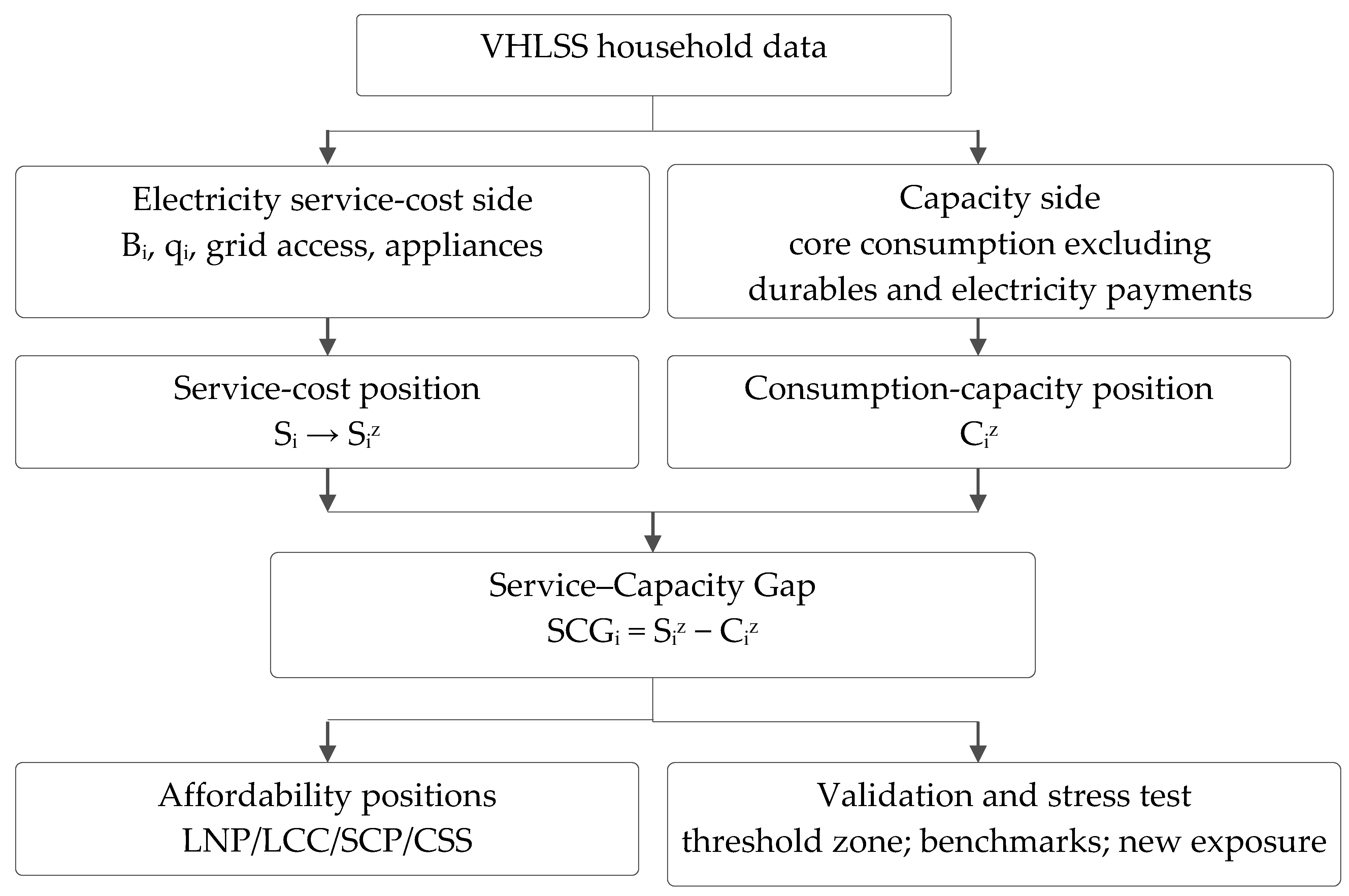
Table 1 shows the analytical payoff of the SCG framework. Existing diagnostics usually capture one side of the affordability problem: high burden, low capacity, low use, or a gap from an external benchmark. SCG instead compares electricity service-cost position with core consumption-capacity position. This comparison opens four diagnostic positions. LCC makes hidden pressure visible when low service-cost still exceeds weak capacity. SCP captures visible service-cost pressure. CSS separates high service-cost from hardship when capacity support is strong. LNP identifies low service-cost non-pressure while avoiding the assumption that low spending is automatically secure. This four-position structure provides the basis for the benchmarking and stress-testing that follow. Figure 1 below summarizes the research flow from household survey data to SCG construction, affordability-position classification, validation, and stress testing.

2.2. Constructing Service–Capacity Gap and Affordability Positions

The first step constructs the electricity service-cost position. Because household surveys do not directly observe electricity-service adequacy, the service-cost side is inferred from electricity consumption, grid access, and appliance/service conditions. This construction is consistent with household electricity-demand research and with recent work linking electricity demand, appliance ownership, and energy-poverty measurement [28,30].

The service-cost equation is specified as:

$$\mathrm{l}\mathrm{n}\left(B_{it}+1\right)={\alpha }_0+{\alpha }_1\mathrm{l}\mathrm{n}\left({\mathrm{kWh}}_{it}+1\right)+{\alpha }_2{\mathrm{Access}}_{it}+{\alpha }_3{\mathrm{Appliance}}_{it}+{\delta }_r+{\lambda }_t+{\epsilon }_{it}.$$

(2)

where ${\mathrm{Access}}_{it}$ denotes grid electricity access, ${\mathrm{Appliance}}_{it}$ captures basic electricity-service conditions, ${\delta }_r$ denotes region fixed effects, and ${\lambda }_t$ denotes year fixed effects. The specification in Equation (2) is used as a reduced-form construction equation for the service-cost position, rather than as a causal electricity-demand model. The selected variables are intended to summarize observed electricity-service intensity and conditions. Electricity use captures the physical intensity of service use; grid access captures basic connection status; appliance quantity captures observed household electricity-service conditions; and region and year fixed effects absorb broad spatial and temporal differences in electricity conditions, tariff environments, and survey-year contexts. Since electricity bills and kWh use are closely related, the construction emphasizes kWh use and service-condition variables in order to reduce the influence of price and billing noise embedded in raw electricity payments.

The fitted value from Equation (2) is defined as the household’s electricity service-cost position:

$$S_{it}=\widehat{\mathrm{l}\mathrm{n}\left(B_{it}+1\right)}$$

(3)

$S_{it}$ captures the revealed electricity service-cost position associated with electricity use, access, and appliance conditions. It is a reduced-form service-cost measure, not the electricity bill. These variables affect the affordability assessment through the service-cost side of SCG: higher electricity use, grid access, and appliance conditions raise the revealed service-cost position, but whether this becomes affordability pressure depends on the household’s consumption-capacity position.

The baseline standardized service-cost position is calculated within each survey year:

$$S_{it}^z={\displaystyle \frac{S_{it}-{\overline{S}}_t}{\sigma \left(S_t\right)}}$$

(4)

where ${\overline{S}}_t$ and $\sigma \left(S_t\right)$ are the year-specific mean and standard deviation of $S_{it}$. A higher $S_{it}^z$ means that household $i$ occupies a higher electricity service-cost position relative to other households in the same survey year.

The capacity side is measured by annual household core consumption excluding durable-goods purchases and electricity payments, converted to a per capita basis. This measure is used as a consumption-capacity benchmark rather than as a complete welfare aggregate. Excluding electricity payments avoids mechanical overlap with the service-cost side, while excluding durable-goods purchases reduces the influence of infrequent large expenditures. Let $C_{it}^{core}$ denote per capita core consumption. The log-transformed capacity measure is:

$$c_{it}=\mathrm{l}\mathrm{n}\left(C_{it}^{core}+1\right)$$

(5)

The standardized core consumption-capacity position is then calculated within each survey year as:

$$C_{it}^z={\displaystyle \frac{c_{it}-{\overline{c}}_t}{\sigma \left(c_t\right)}}$$

(6)

where ${\overline{c}}_t$ and $\sigma \left(c_t\right)$ are the year-specific mean and standard deviation of $c_{it}$ among households observed in year $t$. A higher $C_{it}^z$ indicates a higher relative core consumption-capacity position within the same survey year. To check whether the results depend on the baseline normalization rule, the study applies alternative scaling choices, including pooled z-score standardization and percentile-rank normalization. This follows the indicator-construction principle that normalized indicators should be tested for sensitivity to scaling and aggregation choices [31].

The affordability classification then follows a two-dimensional rule based on service-cost position and SCG. The sign of the standardized service-cost position separates below- and above-average electricity service-cost positions, while the sign of SCG separates households with and without positive service–capacity pressure. The four affordability positions are defined as:

$${\mathrm{Position}}_{it}=\left\{\begin{array}{ll}\mathrm{LNP},& S_{it}^z<0, {\mathrm{SCG}}_{it}\le 0,\\ \mathrm{LCC},& S_{it}^z<0, {\mathrm{SCG}}_{it}>0,\\ \mathrm{SCP},& S_{it}^z\ge 0, {\mathrm{SCG}}_{it}>0,\\ \mathrm{CSS},& S_{it}^z\ge 0, {\mathrm{SCG}}_{it}\le 0.\end{array}\right.$$

(7)

where LNP denotes low service-cost and no pressure, LCC denotes low service-cost but capacity-constrained, SCP denotes service-cost pressure, and CSS denotes capacity-supported service-cost. These positions separate two issues that a single burden ratio may conflate: whether the household has a low or high service-cost position, and whether that position exceeds its relative capacity. The economic logic is that low electricity service cost has different meanings depending on household capacity. For LNP households, capacity is sufficient, so low service cost is more likely to reflect low electricity needs, efficient use, or ordinary consumption choice. For LCC households, capacity is weak, so low service cost may instead reveal a hidden constraint: households may keep electricity spending low because core consumption must be protected first. The same logic applies to high service cost. It indicates pressure in SCP because service cost exceeds capacity support, but it indicates supported service use in CSS because capacity is strong enough to absorb the cost.

The SCG positions are further assessed by testing whether the service-cost–capacity relationship changes across a central threshold zone rather than around a single fixed cutoff. It is not used to classify affordability positions, which are already determined by the joint signs of $S_{it}^z$ and ${\mathrm{SCG}}_{it}$. Instead, the threshold analysis asks whether the capacity–service-cost relationship changes slope as household capacity increases. This validation is needed because the SCG interpretation assumes that stronger household capacity can act as a buffer against service-cost pressure. If this capacity-buffer logic is empirically meaningful, the marginal association between capacity and service-cost position should weaken after households reach a stronger capacity range. A segmented specification is therefore used because it directly estimates the slope before and after a candidate capacity threshold. This follows the logic of threshold and segmented-regression approaches, where slope changes indicate that an empirical relationship differs across ranges of a conditioning variable [32,33].

The main threshold test is estimated in the standardized service-cost–capacity space:

$$S_{it}^z=\alpha +{\beta }_1{C}_{it}^z+{\beta }_2{H}_{it}\left(\kappa \right)+{\lambda }_t+{\delta }_r+{\epsilon }_{it}.$$

(8)

where $H_{it}\left(\kappa \right)=\max \left(C_{it}^z-\kappa ,0\right)$ is the post-threshold capacity term and $\kappa$ denotes the candidate capacity threshold. The coefficient ${\beta }_1$ gives the pre-threshold slope, while ${\beta }_2$ captures the change in slope above $\kappa$. A negative ${\beta }_2$ indicates marginal deceleration, meaning that the association between capacity and service-cost position weakens after the threshold.

To examine whether the standardized threshold is only a normalization artifact, the study also estimates an original-scale threshold check. This check uses the unstandardized service-cost position $S_{it}$ and annual per capita core consumption $C_{it}^{core}$. Because household consumption is measured in nominal terms and changes across survey years, the original-scale threshold is searched by year-specific percentiles of annual per capita core consumption. The original-scale model is specified as:

$$S_{it}=\alpha +{\theta }_1{d}_{it}\left(q\right)+{\theta }_2\max \left\{d_{it}\left(q\right),0\right\}+{\lambda }_t+{\delta }_r+{\epsilon }_{it}.$$

(9)

where $d_{it}\left(q\right)=\mathrm{l}\mathrm{n}\left(C_{it}^{core}+1\right)-{\kappa }_{tq}$ is the year-specific log core-consumption threshold at percentile (q). Candidate thresholds are searched using the same percentile logic in both models. Equation (8) uses percentiles of $C_{it}^z$, while Equation (9) uses the corresponding year-specific percentiles of $C_{it}^{core}$. This paired design links the standardized SCG-space threshold to observed service-cost and core-consumption conditions, so that the capacity-buffer interpretation remains grounded in household economic conditions. Each candidate is evaluated by AIC, BIC, cross-validation RMSE, and bootstrap selection frequency. The consistency between the standardized and original-scale thresholds supports the empirical validity of the SCG boundary as a capacity-buffer point. The selected percentile is therefore read as part of a capacity-buffer zone, not as a fixed welfare cutoff. Similar patterns in the standardized and original-scale checks indicate that the zone is not driven by normalization alone.

2.3. Stress-Testing SCG Under Rising Electricity Costs

After constructing the SCG, the study examines whether rising electricity costs move households across the service-capacity boundary. The exercise is designed as an ex ante stress test rather than a causal estimate of electricity-price reform. Its purpose is to identify households that are not under service–capacity pressure at baseline but become exposed when electricity costs rise. This follows microsimulation and price-shock analysis that evaluates distributional exposure before policy compensation or full behavioral adjustment is modeled [34,35,36].

The empirical results report two electricity-cost shock levels, $s\in \left\{0.20,0.30\right\}$, interpreted as stress-test levels rather than observed one-time tariff-adjustment magnitudes, under two behavioral assumptions. The first is a no-response scenario, where electricity use is held fixed $\left(ϵ=0\right)$. The second is a modest behavioral-response scenario, where electricity use adjusts with a constant elasticity $\left(ϵ=-0.2\right)$. This elasticity is used as a modest response assumption, not as a Vietnam-specific estimate [36]. For household $i$ in year $t$, shocked electricity use and payment are defined as:

$$q_{it}^{s,ϵ}=q_{it}{\left(1+s\right)}^{ϵ}=>B_{it}^{s,ϵ}=B_{it}{\left(1+s\right)}^{1+ϵ}.$$

(10)

When $ϵ=0$, electricity use is fixed, and the electricity bill increases mechanically by $1+s$. When $ϵ=-0.2$, the simulated increase in electricity payment is smaller because households reduce electricity use in response to the cost increase.

The shocked service-cost position is recomputed using the same construction logic as the baseline service-cost measure:

$$S_{it}^{s,ϵ}=\widehat{\mathrm{l}\mathrm{n}\left(B_{it}^{s,ϵ}+1\right)}.$$

(11)

To identify boundary crossing, the shocked service-cost position is standardized against the baseline year-specific distribution:

$$S_{it}^{z,s,ϵ}={\displaystyle \frac{S_{it}^{s,ϵ}-{\bar{S}}_t}{\sigma \left(S_t\right)}}.$$

(12)

Core consumption capacity is held fixed, so the post-shock gap is:

$${\mathrm{SCG}}_{it}^{s,ϵ}=S_{it}^{z,s,ϵ}-C_{it}^z.$$

(13)

New exposure is defined as a transition from a non-positive baseline SCG to a positive post-shock SCG:

$$N{E}_{it}^{s,ϵ}=1\left({\mathrm{SCG}}_{it}\le 0, {\mathrm{SCG}}_{it}^{s,ϵ}>0\right).$$

(14)

where $N{E}_{it}^{s,ϵ}$ denotes new exposure under shock level $s$ and the elasticity assumption $ϵ$. A household is newly exposed if it is not under service–capacity pressure at baseline but crosses into positive SCG after the electricity-cost shock. Exposure rates are reported by baseline affordability position, capacity quintile, and urban-rural status. This design separates mechanical cost exposure $\left(ϵ=0\right)$ from exposure after modest demand adjustment $\left(ϵ=-0.2\right)$, consistent with the two scenarios reported in the results.

3. Data

3.1. Data Source and Analytical Sample

This study uses household-level data from the Vietnam Household Living Standards Survey (VHLSS) for 2012, 2014, 2016, 2018, and 2020 [37,38,39,40,41]. The raw variables were drawn from several household questionnaire sections for each survey wave. Household roster and demographic information were taken mainly from Section 01_1B, education-related controls from Section 02_1B, income-source information from Section 04_1B, consumption and core-consumption items from Section 05_1B, and electricity, housing-utility, and appliance information from Section 07_1B. These section-level files were linked, recoded, and harmonized across survey years to construct a pooled household-year dataset. After excluding observations with missing information on electricity use or household consumption, the final analytical sample contains 46,375 household-year observations. The resulting dataset combines electricity use, payment conditions, appliance ownership, consumption capacity, income structure, demographic characteristics, and location, providing the empirical basis for constructing the Service–Capacity Gap, affordability positions, and rising-cost exposure.

3.2. Electricity Use, Access, and Burden Pattern

The 2012–2020 VHLSS dataset contains 46,375 household-year observations linking electricity payments, kWh use, grid access, appliance ownership, consumption, income, demographics, and location. This structure allows the SCG to connect the electricity service-cost side with household consumption capacity, although the survey does not directly observe service adequacy, thermal comfort, appliance efficiency, or coping behavior.

Table 2. Household Electricity Use, Access, and Burden Patterns in Vietnam, 2012–2020.

Metric	2012	2014	2016	2018	2020	Change 2012–2020 (%)
N (households)	9095	9369	9385	9150	9376	3.1
Grid access (%)	100	98	98.7	99.1	99.4	−0.6
kWh	1020	1200	1500	1668	1848	81.2
Electricity bill (1000 VND)	1300	1800	2400	3000	3600	176.9
Basic electric appliance quantity	4	4	5	5	7	75
Cooling appliance (%)	88.1	90.7	84.9	94.2	95.8	8.7
High-load appliance (%)	87.2	88.8	94.4	94.3	95.5	9.6
Electricity expenditure share by total consumption quintile
– Q1	2.51	2.77	3.28	4.09	4.58	82.8
– Q2	2.31	2.88	3.59	3.98	4.25	84.3
– Q3	2.43	3.03	3.56	3.87	4.15	71
– Q4	2.47	3.01	3.39	3.52	3.85	55.6
– Q5	2.34	2.69	2.93	2.92	3.35	43.1

Notes: Electricity expenditure shares use total household consumption quintiles. Monetary values are annual household totals.

summarizes the main electricity access, use, payment, appliance, and burden patterns, while

Table A1. Household Socio-demographic Conditions by Survey Year, 2012–2020.

Variables	2012	2014	2016	2018	2020
Observations	9095	9369	9385	9150	9376
Urban households (%)	29.6	29.7	30.1	30	32.9
Mean household size	3.88	3.83	3.81	3.73	3.69
Mean dependency ratio	0.6	0.5	0.64	0.66	0.68
Mean head age	50	50	51.7	52.3	51
Female head (%)	25.2	-	25.1	25.4	26.2
Median total household consumption	54,693	61,910	68,104	77,756	88,194
Median per capita core consumption	13,663	15,696	17,345	19,735	23,152
Median per capita income	19,844	23,657	28,222	36,100	41,920

in Appendix A reports additional socio-demographic characteristics.

Table 2 shows a clear post-access electricity transition. Grid access was already nearly universal throughout 2012–2020, while household electricity use and appliance ownership continued to expand. Median annual electricity use increased from 1020 to 1848 kWh, and the median number of basic electric appliances rose from 4 to 7. Cooling and high-load appliance ownership also remained high and increased over time. These patterns suggest that the relevant affordability issue is no longer only whether households are connected to electricity, but whether they can sustain increasingly electricity-dependent household services.

The cost side increased more sharply than electricity use. Median annual electricity bills rose from 1300 to 3600 thousand VND, compared with a smaller increase in kWh. Electricity expenditure shares also rose across all consumption quintiles, but the increase was stronger among lower-consumption households. The Q1 burden increased from 2.51% to 4.58%, while the Q5 burden increased from 2.34% to 3.35%, widening the Q1–Q5 gap from 0.17 to 1.23 percentage points. This increase was not distributionally neutral. Lower-consumption households experienced a larger rise in the relative weight of electricity payments. This is why payment pressure needs to be interpreted together with household consumption capacity.

4. Results

4.1. Service–Capacity Position Construction

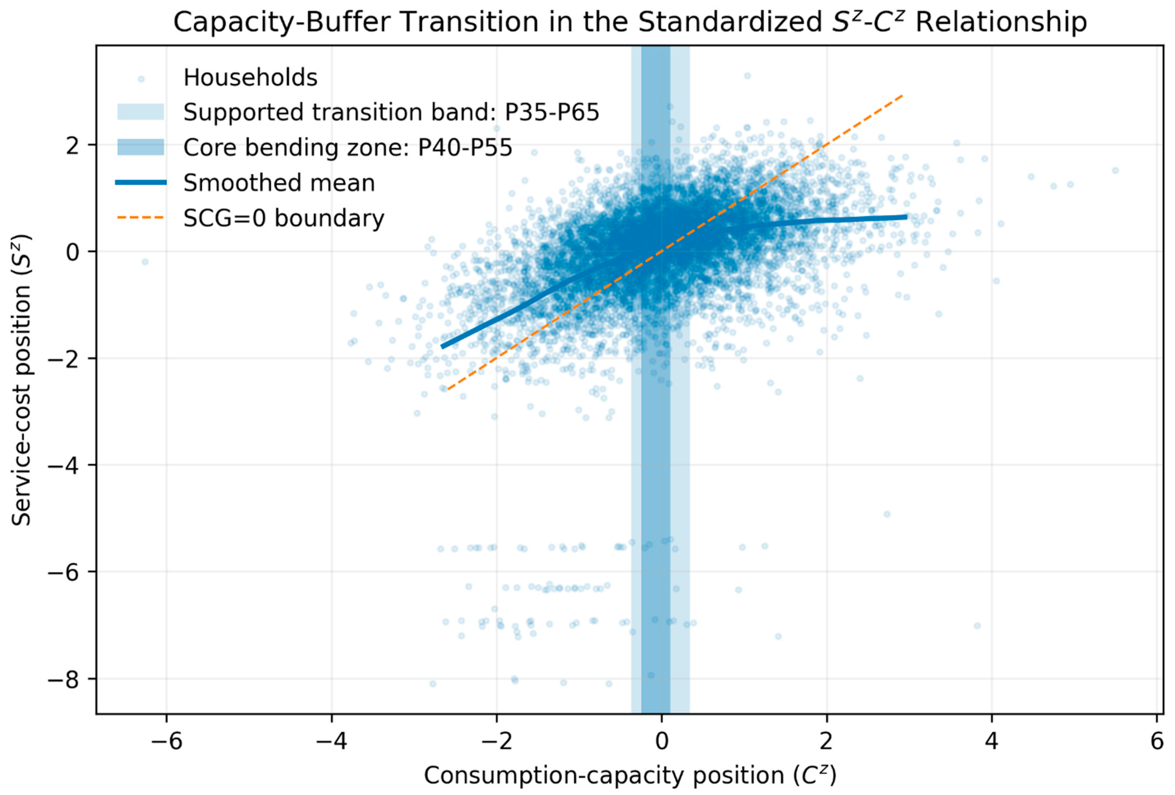
The electricity service-cost position, $S_{it}$, is obtained from the fitted service-cost model in Equation (3) and standardized as $S_{it}^z$ following Equation (4). The core consumption-capacity position, $C_{it}^z$, is constructed from per capita core consumption following Equations (5) and (6). The Service–Capacity Gap then compares these two positions as ${\mathrm{SCG}}_{it}=S_{it}^z-C_{it}^z$, as defined in Equation (1). A positive SCG indicates service–capacity pressure, whereas a non-positive SCG indicates capacity support. The threshold-zone analysis tests whether the standardized $S_{it}^z \mathrm{a}\mathrm{n}\mathrm{d} C_{it}^z$ relationship contains a meaningful slope change. A lower post-threshold slope in Equation (8) means that additional capacity is less strongly associated with a higher service-cost position. To check whether this pattern depends on standardization, Equation (9) repeats the test on the original scale, using S_it and annual per capita core consumption.

Table 3. Construction of Electricity Service-Cost Position.

Variable	Coefficient
ln(kWh + 1)	0.918 ***
	(0.007)
Grid electricity access	0.811 ***
	(0.048)
Basic electric appliance quantity	0.024 ***
	(0.001)
Year FE	Yes
Region FE	Yes
Observations	46,375
R-squared	0.924

Notes: Basic electric appliance quantity is a count-based proxy for appliance/service conditions, constructed from VHLSS-recorded electricity-related assets such as phones, televisions, refrigerators, air conditioners, fans, water heaters, and electric cooking appliances. Robust standard errors are reported in parentheses; *** p < 0.01. VIF: ln(kWh + 1) = 2.10; grid access = 1.61; appliance quantity = 1.41.

reports the construction of $S_{it}$;

Table 4. Within-Year Service-Capacity Positions.

Metric	n	Median Sz	Median Cz	Median SCG	Positive SCG (%)	Median kWh	Median Electricity Bill	Median Core Consumption	Median Income
Overall	46,375	0.134	−0.011	0.102	54.81	408	660	17,698	28,804
Quintile by Cz
– Q1	9276	−0.558	−1.242	0.8	82.91	171	240	8245	12,122
– Q2	9275	−0.032	−0.497	0.464	75.57	318	500	13,092	21,410
– Q3	9274	0.19	−0.011	0.199	63.05	425	680	17,507	28,525
– Q4	9275	0.357	0.483	−0.131	40.14	533	880	23,458	37,588
– Q4	9275	0.545	1.249	−0.786	12.38	750	1300	37,971	56,200
By year
– 2012	9095	0.073	−0.022	0.074	53.29	288	360	13,663	19,844
– 2014	9369	0.157	0.003	0.114	55.99	344	510	15,696	23,657
– 2016	9385	0.17	−0.017	0.106	55	420	672	17,345	28,222
– 2018	9150	0.145	−0.013	0.107	55.37	480	840	19,735	36,100
– 2020	9376	0.099	−0.007	0.108	54.36	560	1068	23,152	41,920

Notes: Original-scale variables are annual per capita measures. Core consumption excludes durables and electricity payments. Monetary values are nominal thousand VND; electricity use is kWh per capita.

examines the service–capacity gradient;

Table 5. Marginal Capacity Threshold-Zone Diagnostics.

Item	Estimate 1 (Standardized)	Estimate 2 (Original-Scale)
Outcome	Sz	Sit
Capacity variable	Cz	$ln{C}_{it}^{core}$
Supported transition band	P35–P65	P35–P65
Core bending zone	P40–P55	P40–P55
Bootstrap mass in P35–P65 (%)	90.0	80.0
Pre-threshold slope in core zone	0.609–0.679	1.145–1.278
Change in slope above threshold in core zone	−0.471 to −0.458	−0.893 to −0.867
Post-threshold slope in core zone	0.151–0.208	0.278–0.385
Marginal slope reduction in core zone (%)	69.3–75.1	69.9–75.8
Minimum AIC within transition band	−14,027.0	−4815.7
Minimum BIC within transition band	−13,922.1	−4710.7
CV RMSE around core zone	≈0.886	≈0.988
Year fixed effects	Yes	Yes
Region fixed effects	Yes	Yes
Observations	46,375	46,375

Notes: S^z and C^z are standardized within each survey year. Original-scale uses unstandardized S_it and log annual per capita core consumption. Zone ranges use bootstrap concentration, slope deceleration, and model fit. See Table A2 and Table A3 in Appendix A.

reports both standardized and original-scale threshold-zone diagnostics;

Table 6. 2012-Baseline Service-Capacity Positions.

Year	n	Mean Sz|2012	Mean Cz|2012	Mean SCGBase2012	Positive SCGBase2012 (%)	Corr. with Baseline SCG	Median Electricity Bill Change (%)	Median Core Consumption Change (%)
Baseline 2012	9095	0	0	0	53.29	1	0	0
2014	9369	0.209	0.216	−0.007	58.12	0.956	41.7	14.9
2016	9385	0.534	0.41	0.124	61.7	0.979	86.7	27
2018	9150	0.792	0.629	0.163	62.23	0.987	133.3	44.4
2020	9376	1.077	0.901	0.175	61.58	0.998	196.6	69.4

Notes: The 2012-baseline positions use the 2012 mean and standard deviation, z_it²⁰¹² = (x_it − μ₂₀₁₂)/σ₂₀₁₂. The two original-scale columns report percentage changes in median annual per capita values relative to 2012.

provides a 2012-baseline check; and Figure 2 visualizes the standardized service-cost–capacity relationship.

Table 3 reports the fitted service-cost construction. The coefficient on ln(kWh + 1) is large and positive, at 0.918, while grid access and basic appliance ownership are also positively associated with the fitted position. These estimates anchor $S_{it}$ in observed electricity use and service conditions. Compared with the electricity bill alone, $S_{it}$ is preferable because it combines payment with kWh use, access, and appliance conditions, thereby representing the household’s revealed service-cost position. The high R² of 0.924 is expected in this construction step and indicates that the measure summarizes electricity service-cost conditions well.

Table 4 shows that higher household capacity is associated with higher electricity use and payment, but lower service–capacity pressure. Across C^z quintiles, median kWh increases from 171 in Q1 to 750 in Q5, and median electricity bill rises from 240 to 1300 thousand VND. This is consistent with the expectation that households with stronger consumption capacity can sustain more electricity-service use. However, the positive-SCG share moves in the opposite direction, falling sharply from 82.91% in Q1 to 12.38% in Q5. The year profile gives the same measurement message from another angle: median kWh and electricity bills rise steadily from 2012 to 2020, while the positive-SCG share remains relatively stable, around 53–56%. These patterns show why electricity affordability cannot be inferred from use or payment levels alone. Low kWh or a low bill may still coexist with weak capacity and positive SCG, while higher use or a higher bill may be supported by stronger capacity. Table 4 establishes the empirical logic of the service–capacity comparison: affordability pressure depends on the relationship between service-cost position and capacity position, not on either side alone.

The diagnostics support a zone-based interpretation of the marginal capacity threshold in Table 5. Bootstrap selections are concentrated within the broader P35–P65 transition band, accounting for 90.0% of selections in the standardized model and 80.0% in the original-scale model, while the strongest bending occurs around P40–P55. In this core zone, the standardized specification shows a marginal slope reduction of 69.3–75.1%, and the original-scale specification gives a similar reduction of 69.9–75.8%. The S^z and C^z relationship therefore changes materially as consumption capacity increases: after the central bending zone, additional capacity is less strongly associated with higher service-cost position, implying a stronger capacity buffer and lower relative pressure. The similarity between the standardized and original-scale results also suggests that the construction remains anchored in real electricity and consumption conditions, rather than being a normalization artifact. Full candidate-level results in

Table A2. Full Threshold Search: Standardized S^z and C^z.

Candidate Threshold	κ	β1	β2	β1 + β2	Slope Reduction (%)	AIC	BIC	CV RMSE	Bootstrap (%)
P30	−0.497	0.739	−0.496	0.243	67.1	−13,947	−13,842	0.888	0
P35	−0.369	0.707	−0.482	0.226	68.1	−13,987	−13,882	0.887	30
P40	−0.246	0.679	−0.471	0.208	69.3	−14,012	−13,907	0.886	10
P45	−0.127	0.654	−0.464	0.19	70.9	−14,025	−13,920	0.886	10
P50	−0.011	0.631	−0.459	0.172	72.8	−14,027	−13,922	0.886	10
P55	0.107	0.609	−0.458	0.151	75.1	−14,022	−13,918	0.886	10
P60	0.224	0.589	−0.459	0.13	77.9	−14,009	−13,904	0.886	0
P65	0.348	0.57	−0.464	0.106	81.4	−13,987	−13,882	0.886	20
P70	0.483	0.551	−0.472	0.078	85.8	−13,951	−13,846	0.886	0
P75	0.625	0.532	−0.484	0.048	91	−13,904	−13,799	0.887	10
P80	0.791	0.512	−0.502	0.01	98	−13,833	−13,728	0.887	0
P85	0.985	0.492	−0.528	−0.036	107.3	−13,736	−13,631	0.888	0
P90	1.249	0.468	−0.569	−0.101	121.6	−13,588	−13,483	0.89	0

and

Table A3. Full Threshold Search: Original-scale S_it and C^core.

Candidate Threshold	κtq	θ1	θ2	θ1 + θ2	Slope Reduction (%)	AIC	BIC	CV RMSE	Bootstrap (%)
P30	κt,30	1.391	−0.941	0.45	67.6	−4735	−4630	0.989	10
P35	κt,35	1.331	−0.913	0.419	68.6	−4769	−4664	0.989	20
P40	κt,40	1.278	−0.893	0.385	69.9	−4796	−4691	0.988	10
P45	κt,45	1.231	−0.882	0.35	71.6	−4816	−4711	0.988	10
P50	κt,50	1.187	−0.873	0.314	73.5	−4816	−4711	0.988	10
P55	κt,55	1.145	−0.867	0.278	75.8	−4803	−4698	0.988	10
P60	κt,60	1.107	−0.869	0.238	78.5	−4788	−4683	0.988	0
P65	κt,65	1.071	−0.879	0.192	82.1	−4766	−4661	0.988	20
P70	κt,70	1.034	−0.894	0.14	86.5	−4730	−4625	0.988	10
P75	κt,75	0.998	−0.917	0.081	91.9	−4684	−4579	0.989	0
P80	κt,80	0.961	−0.952	0.009	99	−4615	−4510	0.989	0
P85	κt,85	0.923	−1.001	−0.078	108.5	−4520	−4415	0.99	0
P90	κt,90	0.877	−1.077	−0.2	122.8	−4366	−4261	0.992	0

in Appendix A confirm that adjacent central thresholds produce similar diagnostics.

Figure 2 visualizes the same bending around the shaded central range, especially near the SCG boundary. The threshold-zone evidence therefore supports the SCG-based classification as a structured service-cost–capacity relationship, not an arbitrary split of standardized scores. The 45-degree line represents S^z = C^z: households above the line have positive SCG, while households below the line have capacity support. The dispersion around this boundary shows that S^z and C^z move together but not proportionally, reinforcing that affordability pressure depends on the distance between the two positions rather than on either position alone.

Table 6 shows that the SCG pattern remains broadly stable when the time reference is fixed to the 2012 distribution. The correlation with the baseline SCG remains high, from 0.956 in 2014 to 0.998 in 2020, indicating that the anchored version preserves the main ordering of households. However, the fixed-baseline check also shows why it is less suitable as the main classification measure. Mean S^z|2012 rises from 0.000 to 1.077, while mean C^z|2012 rises from 0.000 to 0.901. Median electricity bills increase by 196.6%, compared with a 69.4% increase in median core consumption. The anchored version mixes household position with the broader time shift in electricity costs and consumption capacity. Table 4 is more appropriate for the main SCG classification because it compares S^z and C^z within the same survey year, using that year’s updated electricity and consumption distributions.

4.2. Household Profiles of Affordability Positions

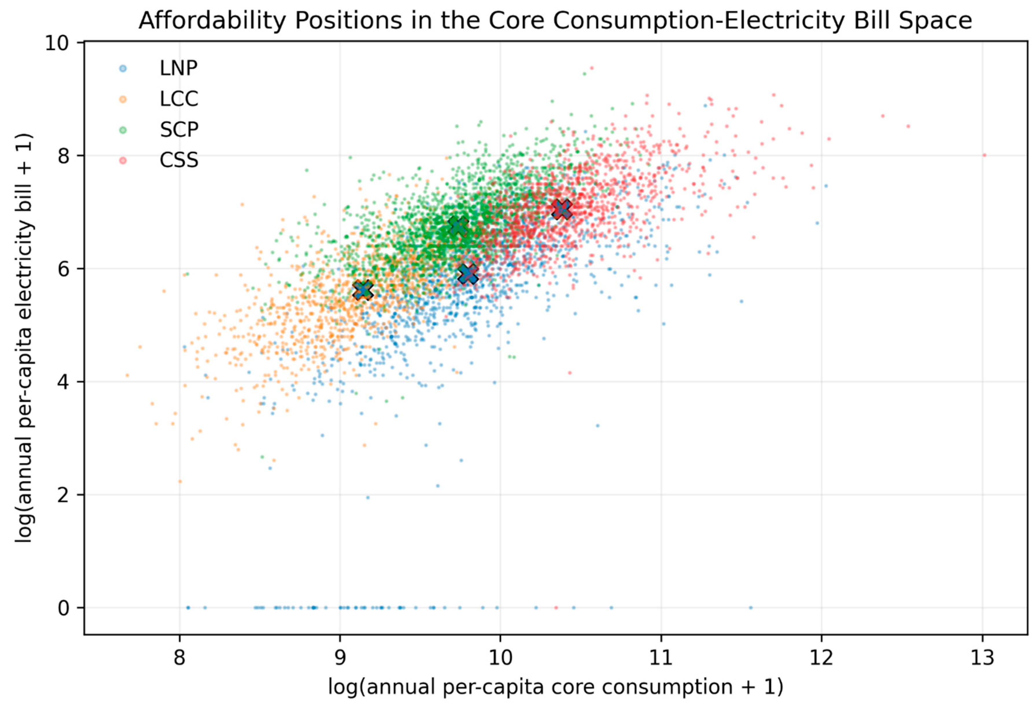
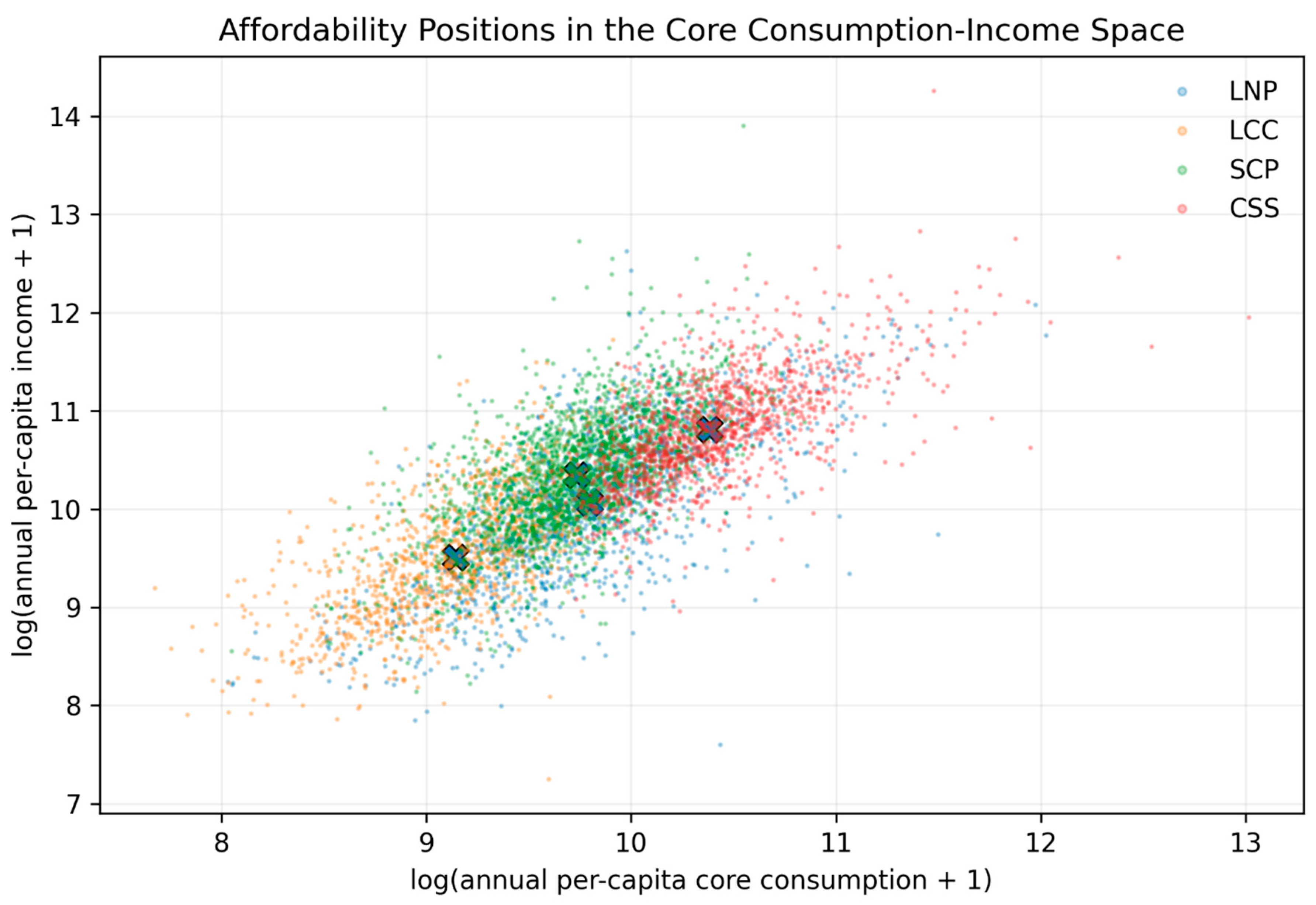
After constructing and validating the SCG boundary, this subsection examines what the four affordability positions mean empirically. Following the two-dimensional rule in Equation (7), (S^z) separates low and high service-cost positions, while SCG separates service–capacity pressure from capacity support to classify LNP, LCC, SCP, and CSS. The analysis links these SCG-based affordability positions to household profiles and to their spatial–temporal distribution. It asks whether LNP, LCC, SCP, and CSS are associated with different electricity-service conditions, income structures, and demographic pressures. Because the SCG position variable is unordered with four categories, the profile analysis uses a multinomial logit model. The estimation includes cooling and high-load appliance indicators, income-source intensities, household demographic controls, and region and year fixed effects.

Table 7. Affordability Positions.

	LNP	LCC	SCP	CSS
Position	Low service-cost non-pressure	Low service-cost but capacity-constrained	Service-cost pressure	Capacity-supported service-cost
Rule	Sᶻ < 0, SCG ≤ 0	Sᶻ < 0, SCG > 0	Sᶻ ≥ 0, SCG > 0	Sᶻ ≥ 0, SCG ≤ 0
n	11,342	8443	16,975	9615
Share (%)	24.46	18.21	36.6	20.73
Median Sz	−0.637	−0.416	0.533	0.436
Median Cz	0.028	−1.061	−0.08	1.003
Median SCG	−0.695	0.508	0.633	−0.462
Median kWh	234	187	540	660
Median electricity bill	367	275	850	1150
Median core consumption	17,966	9344	16,902	32,285
Median income	23,556	13,490	31,223	49,667

Notes: Values are pc thousand VND; kWh is pc annual use.

summarizes the four positions and their original-scale profiles.

Table 8. Affordability Position Distribution by Year and Region.

Group	n	LNP (%)	LCC (%)	SCP (%)	CSS (%)
Survey year
– 2012	9095	28.99	17.94	35.35	17.71
– 2014	9369	20.57	20.11	35.88	23.44
– 2016	9385	21.98	18.03	36.97	23.02
– 2018	9150	23.73	18.17	37.19	20.91
– 2020	9376	27.13	16.77	37.6	18.5
Urban-rural status
– Rural	32,238	27.88	23.3	34.63	14.19
– Urban	14,137	16.65	6.58	41.1	35.67
Region
– Red River Delta	9849	15.59	9.45	50.1	24.87
– Northern midlands and mountains	8043	32.45	27.27	26.68	13.6
– North Central and Central Coast	10,220	26.58	21.93	31.96	19.54
– Central Highlands	3232	27.51	28.37	24.04	20.08
– Southeast	5600	17.18	5.18	45.5	32.14
– Mekong River Delta	9431	27.89	19.84	35.03	17.24

describes the distribution of LNP, LCC, SCP, and CSS over time and across regions.

Table 9. Average Marginal Effects for SCG Affordability Positions.

Variable	LNP	LCC	SCP	CSS
Cooling appliance	−0.152 *** (0.007)	−0.108 *** (0.006)	0.156 *** (0.012)	0.104 *** (0.011)
High-load appliance	−0.263 *** (0.009)	−0.174 *** (0.007)	0.247 *** (0.020)	0.190 *** (0.022)
Wage-income intensity (IHS pc, z)	−0.014 *** (0.002)	−0.026 *** (0.002)	−0.000 (0.002)	0.041*** (0.002)
Farm-income intensity (IHS pc, z)	0.006 *** (0.002)	−0.004 ** (0.002)	0.002 (0.002)	−0.004 * (0.002)
Nonfarm-business income intensity (IHS pc, z)	−0.028 *** (0.002)	−0.059 *** (0.002)	0.042 *** (0.002)	0.046 *** (0.002)
Other-income intensity (IHS pc, z)	−0.009 *** (0.002)	−0.021 *** (0.002)	−0.006 *** (0.002)	0.036 *** (0.002)
Urban	−0.042 *** (0.005)	−0.119 *** (0.005)	0.035 *** (0.005)	0.126 *** (0.004)
Household size (z)	−0.151 *** (0.002)	0.036 *** (0.002)	0.167 *** (0.002)	−0.053 *** (0.002)
Dependency ratio (z)	−0.006 *** (0.002)	0.024 *** (0.002)	0.013 *** (0.002)	−0.031 *** (0.002)
Head completed grade (z)	−0.002 (0.002)	−0.003 ** (0.002)	−0.009 *** (0.002)	0.014 *** (0.002)
Head age (z)	−0.015 *** (0.002)	0.004 ** (0.002)	0.023 *** (0.002)	−0.012 *** (0.002)
Female head	0.025 *** (0.005)	0.014 *** (0.005)	−0.025 *** (0.005)	−0.014 *** (0.005)
Year FE	Yes	Yes	Yes	Yes
Region FE	Yes	Yes	Yes	Yes
Observations	46,375	46,375	46,375	46,375

Notes: Average marginal effects are from a multinomial logit model with LNP, LCC, SCP, and CSS as unordered outcomes. MNL coefficients are in Table A4 in Appendix A. SEs are in parentheses. IHS = inverse hyperbolic sine; pc = per capita; z = standardized. *** p < 0.01, ** p < 0.05, * p < 0.10.

reports average marginal effects from the multinomial-logit model in

Table A4. Multinomial Logit Coefficients for Affordability Positions.

Variable	LNP vs. LCC	SCP vs. LCC	CSS vs. LCC
Cooling appliance	−0.082 * (0.047)	1.488 *** (0.066)	1.532 *** (0.085)
High-load appliance	−0.204 *** (0.049)	2.413 *** (0.098)	2.612 *** (0.159)
Wage-income intensity (IHS pc, z)	0.108 *** (0.018)	0.216 *** (0.017)	0.443 *** (0.020)
Farm-income intensity (IHS pc, z)	0.055 *** (0.020)	0.028 (0.019)	0.006 (0.021)
Nonfarm-business income intensity (IHS pc, z)	0.231 *** (0.021)	0.604 *** (0.019)	0.726 *** (0.021)
Other-income intensity (IHS pc, z)	0.101 *** (0.017)	0.149 *** (0.016)	0.372 *** (0.019)
Urban	0.561 *** (0.048)	1.048 *** (0.045)	1.641 *** (0.047)
Household size (z)	−1.017 *** (0.022)	0.452 *** (0.018)	−0.437 *** (0.022)
Dependency ratio (z)	−0.192 *** (0.017)	−0.129 *** (0.015)	−0.351 *** (0.019)
Head completed grade (z)	0.018 (0.014)	−0.001 (0.016)	0.104 *** (0.017)
Head age (z)	−0.108 *** (0.016)	0.058 *** (0.016)	−0.087 *** (0.019)
Female head	0.040 (0.042)	−0.215 *** (0.043)	−0.203 *** (0.047)
Year FE	Yes	Yes	Yes
Region FE	Yes	Yes	Yes
Observations	46,375	46,375	46,375

Notes: Coefficients are multinomial logit estimates $Pr\left({\mathrm{P}\mathrm{o}\mathrm{s}\mathrm{i}\mathrm{t}\mathrm{i}\mathrm{o}\mathrm{n}}_{it}=m\mid Z_{it}\right)={\displaystyle \frac{\mathrm{e}\mathrm{x}\mathrm{p}\left({\eta }_{itm}\right)}{\sum _{j\in M}\mathrm{e}\mathrm{x}\mathrm{p}\left({\eta }_{itj}\right)}}$ with ${\eta }_{itLCC}$ normalized to zero and, for m ≠ LCC, ${\eta }_{itm}$ = ${\rho }_{0m}$ + ${\rho }_{1m}{\mathrm{C}\mathrm{o}\mathrm{o}\mathrm{l}\mathrm{i}\mathrm{n}\mathrm{g}}_{it}$ + ${\rho }_{2m}{\mathrm{H}\mathrm{i}\mathrm{g}\mathrm{h}\mathrm{L}\mathrm{o}\mathrm{a}\mathrm{d}}_{it}$ + ${\varphi }_m^{\prime {\mathrm{I}\mathrm{n}\mathrm{c}\mathrm{o}\mathrm{m}\mathrm{e}\mathrm{S}\mathrm{o}\mathrm{u}\mathrm{r}\mathrm{c}\mathrm{e}\mathrm{s}}_{it}}$ + $X_{it}^{\prime {\rho }_m}$ + ${\delta }_{rm}$ + ${\lambda }_{tm}$. Standard errors are in parentheses. IHS = inverse hyperbolic sine; pc = per capita; z = standardized. *** p < 0.01, * p < 0.10.

in Appendix A. Figure 3 and Figure 4 then locate them in core consumption–electricity bill and core consumption–income spaces.

Table 7 shows that the four SCG positions are not a simple ranking by electricity use, electricity bills, income, or core consumption. The key distinction is whether a given service-cost position is supported by household consumption capacity. Positive-SCG households account for 54.81% of the sample, including LCC and SCP, while non-positive-SCG households account for 45.19%, including LNP and CSS. The original-scale profiles confirm that low electricity use does not always mean affordability security, and high electricity use does not always mean hardship. The main empirical value of the SCG classification is therefore to separate service-cost position from capacity support, preventing both low-use and high-use households from being misclassified when capacity is ignored.

LCC is the clearest hidden capacity-constrained group. It has low electricity use and a low median electricity bill, at 187 kWh and 275 thousand VND, but it also has the weakest capacity profile, with median (C^z = −1.061), core consumption of 9344 thousand VND, and income of 13,490 thousand VND. Its positive median SCG of 0.508 shows that even a low service-cost position can exceed household capacity. This is the type of hidden affordability pressure that a burden-ratio or bill-size indicator may understate.

SCP represents visible service-cost pressure. It has above-average service cost, with a median (S^z = 0.533), higher electricity use of 540 kWh, and a median electricity bill of 850 thousand VND. However, its capacity position remains weak relative to service cost, with a median (C^z = −0.080), producing the highest median SCG of 0.633. SCP therefore corresponds most closely to the conventional idea of affordability stress: higher electricity payments are not sufficiently backed by household consumption capacity.

CSS shows the opposite case of capacity-supported high service cost. It has the highest electricity use and electricity bill, at 660 kWh and 1150 thousand VND, but also the strongest capacity profile, with median (C^z = 1.003), core consumption of 32,285 thousand VND, and income of 49,667 thousand VND. Its negative median SCG of −0.462 indicates that high service cost is supported by household capacity rather than automatically translating into pressure.

LNP is substantively important because it prevents low electricity use from being automatically interpreted as hidden deprivation. Like LCC, LNP has a low service-cost profile, but its capacity conditions are clearly stronger: median (C^z = 0.028), core consumption of 17,966 thousand VND, and income of 23,556 thousand VND. Its negative median SCG of −0.695 indicates low service cost without observed capacity pressure. The contribution of SCG is not only to identify hidden pressure in LCC, but also to separate LNP from constrained low-use households that conventional low-use or benchmark-based indicators may otherwise group together.

Table 8 shows that the four-position structure is relatively stable over time but strongly differentiated by location. SCP remains the largest position in every survey year, rising slightly from 35.35% in 2012 to 37.60% in 2020, while LCC stays within a narrow range of 16.77–20.11%. This suggests that positive service–capacity pressure is not driven by a single survey wave. The spatial pattern is clearer: rural households are more concentrated in LNP and LCC, at 27.88% and 23.30%, while urban households are concentrated in SCP and CSS, at 41.10% and 35.67%. Regional differences reinforce this contrast. Northern midlands and mountains and Central Highlands have the highest LCC shares, at 27.27% and 28.37%, indicating stronger hidden capacity constraints, whereas the Red River Delta and Southeast have much lower LCC shares but higher SCP and CSS shares. The Red River Delta has the highest SCP share, at 50.10%, while the Southeast has the highest CSS share, at 32.14%. Thus, more developed or urbanized areas do not simply move into affordability security. Instead, they shift toward higher service-cost positions, which are capacity-supported for some households but remain a pressure for others.

Figure 3 and Figure 4 make the original-scale separation between the four positions more visible. LCC is located in the low-capacity and low-bill area, showing that its low electricity use occurs under weak consumption capacity. SCP moves upward toward higher electricity bills, but its core consumption and income do not rise enough to provide clear capacity support. CSS occupies the high-capacity side: its electricity bills are higher, but they are matched by stronger core consumption and income. LNP is the most visually ambiguous group. From the electricity side, it looks like a low-use and low-bill group, which could be mistaken for constrained low service use. From the capacity side, however, it is not as weak as LCC: its core consumption is much higher and closer to the middle of the distribution. This explains why LNP needs the SCG rule to be identified correctly. It is not defined by low electricity use alone, but by low service cost combined with non-positive service–capacity pressure.

Table 9 shows that appliance-related electricity demand is the strongest separator between low and high service-cost positions, and this pattern remains stable in the one-vs-rest LPM estimates reported in

Table A5. One-vs-Rest Linear Probability Estimates for Affordability Positions.

Variable	LNP	LCC	SCP	CSS
Cooling appliance	−0.119 *** (0.007)	−0.104 *** (0.007)	0.146 *** (0.008)	0.076 *** (0.007)
High-load appliance	−0.169 *** (0.008)	−0.125 *** (0.007)	0.210 *** (0.009)	0.084 *** (0.008)
Wage-income intensity (IHS pc, z)	−0.018 *** (0.002)	−0.028 *** (0.002)	0.005 ** (0.002)	0.040 *** (0.002)
Farm-income intensity (IHS pc, z)	0.003 (0.002)	−0.001 (0.002)	0.001 (0.003)	−0.003 (0.002)
Nonfarm-business income intensity (IHS pc, z)	−0.035 *** (0.002)	−0.056 *** (0.002)	0.045 *** (0.002)	0.046 *** (0.002)
Other-income intensity (IHS pc, z)	−0.004 * (0.002)	−0.025 *** (0.002)	−0.005 ** (0.002)	0.034 *** (0.002)
Urban	−0.066 *** (0.005)	−0.100 *** (0.004)	0.012 ** (0.005)	0.154 *** (0.005)
Household size (z)	−0.137 *** (0.002)	0.032 *** (0.002)	0.159 *** (0.002)	−0.053 *** (0.002)
Dependency ratio (z)	−0.014 *** (0.002)	0.027 *** (0.002)	0.012 *** (0.002)	−0.024 *** (0.002)
Head completed grade (z)	−0.002 (0.002)	−0.004 ** (0.002)	−0.007 *** (0.002)	0.012 *** (0.002)
Head age (z)	−0.001 (0.002)	−0.004 ** (0.002)	0.022 *** (0.002)	−0.017 *** (0.002)
Female head	0.042 *** (0.005)	0.004 (0.005)	−0.020 *** (0.005)	−0.026 *** (0.005)
Year FE	Yes	Yes	Yes	Yes
Region FE	Yes	Yes	Yes	Yes
Observations	46,375	46,375	46,375	46,375

Notes: Standard errors are in parentheses. IHS = inverse hyperbolic sine; pc = per capita; z = standardized. *** p < 0.01, ** p < 0.05, * p < 0.10.

in Appendix A. Cooling and high-load appliances reduce the probability of LNP and LCC, but increase the probability of SCP and CSS. The effect of high-load appliances is particularly large: it reduces the probability of LNP by 26.3 percentage points and LCC by 17.4 percentage points, while increasing SCP by 24.7 percentage points and CSS by 19.0 percentage points. The signs and magnitudes separate high-service-cost positions from low-service-cost positions: SCP and CSS are associated with higher electricity-service requirements, whereas LNP and LCC are closer to lower observed service-cost conditions.

The remaining covariates clarify the household profiles behind these positions. LCC is associated with weak capacity support: wage, nonfarm-business, and other-income intensities reduce its probability by 2.6, 5.9, and 2.1 percentage points, while household size and dependency ratio increase it by 3.6 and 2.4 percentage points. SCP is the load-pressure profile: high-load appliances and household size increase its probability by 24.7 and 16.7 percentage points, indicating that electricity-service needs and household scale jointly raise visible pressure. CSS is the capacity-supported profile: urban residence raises its probability by 12.6 percentage points, while wage, nonfarm-business, and other-income intensities increase it by 4.1, 4.6, and 3.6 percentage points. By contrast, household size and dependency ratio reduce it. LNP is the lower-load non-pressure profile: high-load appliances and household size reduce its probability by 26.3 and 15.1 percentage points, while female headship increases it slightly by 2.5 percentage points. Overall, the SCG positions correspond to distinct household conditions of load demand, income support, and demographic pressure.

4.3. Benchmark Validation and Socioeconomic Meaning

The added diagnostic value of SCG lies in its ability to separate two pairs that conventional indicators often conflate: LNP versus LCC on the low service-cost side, and SCP versus CSS on the high service-cost side.

Table 10. Two-Way Benchmarking between Conventional Electricity-Affordability Diagnostics and SCG Positions.

Established Diagnostic Group	Sample Share (%)	LNP	LCC	SCP	CSS
Panel A. Conventional diagnostic groups mapped onto SCG positions
Classic 10% burden by core consumption	3.97	1.90	9.17	81.06	7.87
Classic 10% burden by income	1.21	13.75	18.04	50.89	17.32
High consumption-burden, BurdenC > P75t	25.00	4.81	10.21	70.35	14.63
High income-burden, BurdenY > P75t	25.00	12.64	13.59	53.95	19.81
Low-service-use, kWhpc < P25t	24.93	48.23	46.41	4.59	0.78
Below IEA minimum access benchmark	6.51	80.82	19.18	0.00	0.00
LIHC-type proxy: high burden and low capacity	13.09	4.15	19.51	76.34	0.00
Panel B. SCG positions benchmarked against conventional diagnostics
SCG position share (%)		24.46	18.21	36.6	20.73
Classic 10% burden by core consumption		0.31	2	8.8	1.51
Classic 10% burden by income		0.68	1.2	1.68	1.01
High consumption-burden, BurdenC > P75t		4.92	14.02	48.05	17.64
High income-burden, BurdenY > P75t		12.92	18.67	36.85	23.89
Low-service-use, kWhpc < P25t		49.15	63.53	3.12	0.94
Below IEA minimum access benchmark		21.5	6.86	0	0
LIHC-type proxy: high burden and low capacity		2.22	14.02	27.3	0

Notes: Panel A maps conventionally identified households into SCG positions. Panel B reports the share within each SCG position meeting each conventional diagnostic. P75_t/P25_t are year-specific thresholds. LIHC combines high burden (Burden^C > P75_t) with low capacity (C_z < 0).

benchmarks these four positions against the conventional diagnostics summarized in Table 1. Panel A starts from each conventional diagnostic and shows how flagged households are distributed across LNP, LCC, SCP, and CSS. Panel B starts from each SCG position and reports the share within that position also flagged by each conventional diagnostic.

Table 11. Socioeconomic Profiles of SCG Positions and Conventional Diagnostic Groups.

Group	Median Income pc	Median Core Cons. pc	Bottom Income Q1 (%)	Rural (%)	HH Size	Dependency Ratio	Low Head Education (%)
All households	28,804	17,698	20.00	69.52	3.79	0.66	32.12
Low-service and hidden-constraint profiles
SCG: LNP	23,556	17,966	26.37	79.25	2.86	0.52	42.51
SCG: LCC	13,490	9344	54.86	88.98	4.14	0.85	49.82
kWhpc < P25t	14,373	10,810	51.80	87.95	4.31	0.81	50.42
Below IEA benchmark	10,796	9720	61.03	73.56	3.11	0.70	61.41
High-burden and pressure profiles
SCG: SCP	31,223	16,902	8.84	65.77	4.47	0.75	25.42
SCG: CSS	49,667	32,285	1.58	47.56	3.37	0.49	15.96
BurdenC > P75t	33,708	17,265	11.89	59.80	3.50	0.66	25.05
BurdenY > P75t	22,842	18,391	28.71	63.14	3.35	0.67	30.39
LIHC-type proxy	24,385	12,460	21.38	75.11	3.75	0.76	33.00

Notes: Values are pc thousand VND; low education = Grade ≤ 5.

then examines whether these diagnostic differences correspond to socioeconomic differences in income, core consumption, rural status, household size, dependency, and education.

Table 10 shows the main benchmarking result: SCG agrees with conventional diagnostics when their signals are clear, but adds diagnostic value by resolving two ambiguities that conventional indicators tend to conflate. Low service cost can mean either non-pressure (LNP) or hidden capacity constraint (LCC), while high service cost can mean either affordability pressure (SCP) or capacity-supported service use (CSS). For example, 81.06% of households with a classic 10% burden by core consumption and 76.34% of LIHC-type households fall into SCP, confirming that conventional high-burden diagnostics align closely with visible service-cost pressure. In contrast, low-use diagnostics do not map into a single affordability condition. Among households below the low-service-use threshold, 48.23% are LNP and 46.41% are LCC. Households below the IEA minimum benchmark are also divided between LNP and LCC. Low electricity use may reflect ordinary low demand without affordability pressure, but it may also reflect constrained use caused by weak household capacity. Panel B confirms the same distinction from the SCG side: LNP has a high low-use share but very low LIHC-type risk, whereas LCC combines low service use with stronger capacity constraint. CSS provides the opposite case: it includes some high-burden households but no LIHC-type risk, showing that high service cost does not necessarily imply affordability hardship when capacity support is strong.

Table 11 further shows why this separation has socioeconomic meaning. LCC resembles the low-use benchmark groups more closely than LNP: its median income is 13,490 thousand VND, close to the kWh_pc < P25_t group at 14,373 thousand VND, while LNP is much higher at 23,556 thousand VND. LCC also has a much larger bottom-income-quintile share than LNP, at 54.86% versus 26.37%. Thus, SCG separates low service-cost households with hidden capacity constraints from low service-cost households without the same socioeconomic disadvantage. On the high-cost side, SCP is closer to conventional high-burden and LIHC-type profiles, while CSS has much stronger capacity: median core consumption is 16,902 thousand VND for SCP but 32,285 thousand VND for CSS. This distinction prevents high electricity cost from being read automatically as hardship. Together with the profile estimates in Table 9, these socioeconomic contrasts show that SCG does not only re-label conventional indicators. It separates low-use and high-cost households into groups with different capacity and policy meanings.

4.4. New Exposure Under Rising Electricity Costs

This subsection applies the rising-cost stress test to identify households close to the service–capacity boundary. Following Equations (10)–(14), electricity bills are shocked under 20% and 30% cost increases, the post-shock service-cost position is recalculated, and new exposure is defined as a transition from SCG ≤ 0 at baseline to SCG^s > 0 after the shock.

Table 12. New Exposure by Baseline SCG Position and Cost Shock.

Group	n	Baseline Positive SCG (%)	New Exposure 20% ϵ = 0 (%)	New Exposure 20%, ϵ = −0.2 (%)	New Exposure 30%, ϵ = 0 (%)	New Exposure 30%, ϵ = −0.2 (%)
Affordability position
– LNP	11,342	0	13.3	10.5	19.03	15.09
– CSS	9615	0	20.92	16.9	28.99	23.86
Capacity quintile
– Q1	9276	82.91	3.87	3.12	5.43	4.37
– Q2	9275	75.57	6.18	5.05	8.23	6.89
– Q3	9274	63.05	9.24	7.38	12.73	10.32
– Q4	9275	40.14	12.28	9.91	17.62	14.25
– Q5	9275	12.38	6.38	4.92	9.3	7.36
Urban-rural
– Rural	32,238	57.93	7.39	5.85	10.41	8.4
– Urban	14,137	47.68	8.05	6.59	11.24	9.18

Notes: New exposure is defined as a transition from SCG ≤ 0 at baseline to SCG > 0 after the electricity-cost shock. The no-response and behavioral-response scenarios use ϵ = 0 and ϵ = −0.2, respectively.

reports this transition under two assumptions: a no-response case (ϵ = 0) and a behavioral-response case (ϵ = −0.2).

Table 12 shows that new exposure is concentrated among households that are not under pressure at baseline but have limited distance from the SCG boundary. Among affordability positions, CSS has higher transition risk than LNP: under the 30% no-response scenario, 28.99% of CSS households become newly exposed, compared with 19.03% of LNP households. With behavioral response, these rates fall to 23.86% and 15.09%, but the ranking remains the same. Across capacity quintiles, Q1 has the highest baseline positive SCG share, at 82.91%, but low new exposure because many households are already under pressure. New exposure is highest in Q4, reaching 17.62% under the 30% no-response scenario and 14.25% with behavioral response. Rising electricity costs therefore create transition risk not only among the poorest households, but also among moderate-capacity households that were initially supported but close to the SCG boundary. Thus, rural households carry more existing SCG pressure, whereas urban households show slightly greater boundary-crossing risk under rising electricity costs.

4.5. Measurement Robustness

Measurement robustness is examined to assess whether the main classification in Equation (7) remains stable under alternative measurement choices. This is important because SCG is a constructed diagnostic indicator: it compares standardized service-cost and capacity positions, so the four-position structure should not be driven by one normalization rule, one capacity benchmark, one cutoff rule, or one service-cost specification. The robustness checks cover four dimensions. First, alternative normalization rules compare the baseline within-year z-score with pooled z-score and percentile-rank normalization. Second, alternative capacity benchmarks replace core consumption with total consumption and income. Third, alternative classification cutoffs test whether the four positions depend too strongly on the baseline (S^z ≥ 0) and (SCG > 0) rules. Fourth, an alternative service-side proxy replaces the baseline service-cost position with a reduced-form service-utility measure. The results are summarized in

Table 13. Robustness of Affordability Position Classification.

Specification	Corr. with Baseline Sz	Corr. with Baseline SCG	LNP (%)	LCC (%)	SCP (%)	CSS (%)
Normalization Sit
– Baseline within-year z-score	1.0	1	24.46	18.21	36.6	20.73
– Pooled z-score	0.946	0.991	23.64	19.12	35.82	21.43
– Percentile-rank normalization	0.836	0.826	32.2	17.79	34.21	15.79
Capacity benchmark Cit
– Total consumption capacity	N.A.	0.966	24	18.67	36.62	20.71
– Income capacity	N.A.	0.733	23.98	18.68	35.48	21.84
Classificatory affordability position
– Year-median high S, SCG > 0	N.A.	1	27.6	22.38	32.43	17.59
– Sz ≥ 0, SCG > yearly P60	N.A.	1	30.28	12.38	27.62	29.72
Service-side sensitivity Sit ⟶ Uit
– Reduced-form service-utility proxy U	0.455	0.58	36.34	16.08	34.88	12.69

Notes: N.A. indicates that the comparison is not applicable. The reduced-form service-utility proxy is defined as $\widehat{U_{it}}\equiv \widehat{E}\left(\widehat{S_{it}} |X_{it}^{\prime }, {\delta }_r, {\lambda }_t\right)$. The (U)-based specification replaces the baseline service-cost side with this predicted service-utility proxy.

.

Table 13 shows that the main SCG classification remains stable under alternative measurement choices. Changing the normalization rule has limited effects. The pooled z-score specification remains very close to the baseline, with correlations of 0.946 for S^z and 0.991 for SCG, and only small changes in the four position shares. Percentile-rank normalization produces a larger increase in LNP and a lower CSS share, but the core structure remains: SCP is still the largest position, and LCC remains close to the baseline level. The classification is also robust to alternative capacity benchmarks. Replacing core consumption with total consumption gives an SCG correlation of 0.966 and almost unchanged group shares, while income capacity gives a lower but still meaningful SCG correlation of 0.733. This suggests that the baseline results are not driven by one specific capacity measure.

The sensitivity checks based on alternative cutoffs and the reduced-form service-utility proxy show where the classification is more flexible but still interpretable. Stricter or median-based classification rules change the shares of LNP, LCC, SCP, and CSS, as expected, but they do not remove the central distinction between low service-cost positions and positive service–capacity pressure. The reduced-form service-utility proxy produces the largest shift, with LNP rising to 36.34% and CSS falling to 12.69%, because this specification replaces the observed service-cost side with a household-structure-based proxy. Even under this more restrictive service-side construction, LCC and SCP together still account for about half of the sample. Taken together, the robustness checks support the measurement credibility of SCG. Exact group shares vary with scaling, thresholds, and service-side assumptions, but the four-position structure remains sufficiently stable to indicate a persistent service–capacity mismatch.

5. Discussion

The results place household electricity affordability in a post-access setting. Once connection is nearly universal, the central issue is no longer access alone but whether electricity-service costs are supported by household capacity. Conventional measures remain useful in this setting, but they capture only part of the problem. Burden-ratio and fuel-poverty approaches identify visible payment pressure, whereas low-use and benchmark-based measures are designed to detect possible under-service and hidden deprivation [3,4,9]. The difficulty arises when these signals diverge. The benchmarking results show that SCG agrees with conventional diagnostics when their signals are clear, but adds value where those signals are ambiguous. High-burden and LIHC-type diagnostics align mainly with SCP, while low-use diagnostics split between LNP and LCC. SCG therefore adds a capacity-based reading to conventional diagnostics and is closer to the SDG7 concern with affordable and reliable electricity services under rising costs.

The main conceptual contribution is that SCG changes the object of classification from electricity use or bill size alone to the relationship between service-cost position and consumption-capacity support. The benchmarking and socioeconomic profiles show that this relationship separates low-cost and high-cost households into positions with different welfare meanings. This distinction is clearest on the low service-cost side. LNP and LCC may look similar through electricity use, but LNP has negative SCG, while LCC has positive SCG and weaker core consumption. The socioeconomic profiles reinforce this interpretation: LCC is closer to low-use benchmark groups, whereas LNP has a distinct and less constrained profile. On the high service-cost side, SCP and CSS separate visible pressure from supported higher service use. Similarly, SCP is closer to conventional high-burden and LIHC-type profiles, while CSS is separated by higher income and consumption capacity. In this sense, SCG extends hidden energy-poverty arguments by adding a capacity condition to low-use interpretation, rather than treating all low use as either deprivation or security [9,23]. It also remains consistent with energy-service approaches that interpret electricity as an input into the household functions and services it enables [7]. The unresolved ambiguity is mainly around LNP, because low observed service cost can still conceal restrictions when comfort, housing quality, appliance efficiency, or coping behavior are not observed.

The measurement evidence supports treating SCG as a relative diagnostic rather than a mechanical z-score classification. Since SCG depends on standardized service-cost and capacity positions, scaling and cutoff choices are legitimate concerns for a constructed indicator [31]. The threshold-zone results address this concern by showing that the capacity–service-cost relationship bends within a central transition band, with marginal slope reductions of roughly 69–76% in both standardized and original-scale specifications. This supports a capacity-buffer interpretation, but not a precise welfare cutoff, consistent with threshold and segmented-regression logic [32,33]. Robustness checks further show that the main structure remains close to the baseline when normalization and capacity benchmarks are changed. SCG is therefore best read as a stable relative measure of service–capacity mismatch, not as a direct measure of absolute service adequacy or experienced welfare. This interpretation is important for the benchmarking exercise: SCG does not replace external welfare outcomes, but it organizes established affordability signals into positions with clearer capacity and policy meanings.

The profile estimates and socioeconomic comparisons suggest that LCC should be treated as a low-service but capacity-constrained group, while SCP should be treated as a high-service-cost pressure group. Conversely, LNP should not be classified as vulnerable solely because of low electricity use, and CSS should not be classified as hardship solely because of high electricity costs. CSS and LNP are not under pressure at baseline, but they differ in exposure to rising costs. Under a 30% electricity-cost shock, new exposure is higher for CSS than for LNP, and this ranking remains when behavioral adjustment is allowed. This indicates that rising costs can erode capacity support even among households that appear secure in the baseline classification. This is consistent with distributional energy-price shock studies showing uneven household exposure before compensation or adjustment is fully captured [35,36].

In Vietnam, this distinction is relevant to an electricity-reform context in which household protection, distributional effects, subsidy design, and perceptions of reasonable electricity bills are closely linked to both affordability and provision-cost concerns [42,43,44,45]. SCG adds to this policy context by showing that affordability targeting should not rely only on poverty status, bill size, or low electricity use. In policy terms, LCC calls for targeted affordability support and basic-service protection, SCP for temporary bill relief, tariff smoothing, or efficiency support, LNP for screening rather than automatic low-use subsidies, and CSS for monitoring under rising-cost exposure.

This can be translated into a practical eligibility rule that prioritizes LCC households for support while excluding LNP households from automatic low-use targeting. A household should be treated as an LCC priority case when the following conditions are met:

−

The household is in a low-use position. In the 2020 data, the year-specific P25 of per capita electricity use is about 342 kWh per person per year, or roughly 28–29 kWh per person per month. Households below this threshold, or below the minimum-use benchmark, should be screened for LCC risk.

−

Low electricity use is accompanied by weak capacity. The preferred rule is positive SCG. Where full SCG calculation is not available, per capita core consumption below the P35–P40 range of the current year’s distribution can be used as a practical proxy. In the 2020 data, this corresponds approximately to 19–20 million VND per person per year, or about 1.6–1.7 million VND per person per month. Households below this range should be treated as likely hidden-constraint cases.

−

Priority should be increased for rural households, households with large size or high dependency ratios, and households located in the Central Highlands and the Northern midlands and mountains.

−

Low-use households with non-positive SCG, or with per capita core consumption above the current-year P40 threshold, should be screened as LNP and excluded from automatic low-use subsidy targeting. In the 2020 data, this P40 threshold is about 20 million VND per person per year.

6. Conclusions

This study developed a Service–Capacity Gap (SCG) approach to examine household electricity affordability under rising costs in Vietnam. The core argument is that affordability should not be assessed only from electricity bills, electricity use, or income position, but from whether a household’s electricity service-cost position is supported by its core consumption capacity. Using VHLSS 2012–2020 data, the study documents a post-access cost transition: median annual electricity use rose from 1020 to 1848 kWh, while median annual electricity bills increased from 1300 to 3600 thousand VND. This divergence shows why rising electricity payments need to be interpreted through household capacity rather than electricity use alone.

The main finding is that SCG adds diagnostic value by resolving two ambiguities that conventional indicators tend to conflate. Low service-cost can mean either low service-cost non-pressure (LNP) or hidden capacity constraint (LCC), while high service-cost can mean either service-cost pressure (SCP) or capacity-supported service-cost (CSS). The four positions are substantial in size: SCP is the largest group at 36.60%, followed by LNP at 24.46%, CSS at 20.73%, and LCC at 18.21%. Benchmark comparisons show that SCG is consistent with conventional diagnostics where their signals are clear, but it adds information where those signals are ambiguous. Low-use indicators split between LNP and LCC, while high-burden and LIHC-type diagnostics align more closely with SCP. Socioeconomic profiles further show that these are not only different labels: LCC is much more capacity-constrained than LNP, and CSS has much stronger capacity than SCP.

The policy implication is to combine current-pressure targeting with boundary monitoring. LCC and SCP require priority because they already show positive SCG, but they represent different problems: hidden low-service-cost constraint in LCC and visible service-cost pressure in SCP. By contrast, LNP should not be classified as vulnerable solely because of low electricity use, and CSS should not be treated as hardship solely because of high electricity costs. Rising costs can nevertheless move non-pressure households across the SCG boundary. Under a 30% cost shock, new exposure reaches 28.99% for CSS and 19.03% for LNP in the no-response case, with the same ranking under behavioral adjustment. For Vietnam, this means that affordability policy should not rely only on poverty status, bill size, or low electricity use, but should also monitor households near the service–capacity boundary.

A key limitation is that SCG is a relative diagnostic, not a direct measure of absolute service adequacy or experienced welfare. The main unresolved issue concerns unobserved service conditions, including thermal comfort, dwelling quality, appliance efficiency, tariff exposure, and coping behavior. This matters especially for interpreting LNP, where low service cost may still conceal restrictions that are not observed in the survey. The stress test also captures ex ante boundary crossing rather than causal behavioral responses to electricity-price changes. Future work can extend the framework by combining household surveys with weather, housing quality, electricity pricing structures, subjective bill-stress indicators, and panel or quasi-experimental evidence, as well as by applying SCG to other household energy services and country contexts.

References

1. Bhatia, M.; Angelou, N. Beyond Connections: Energy Access Redefined; World Bank: Washington, DC, USA, 2015. [Google Scholar]
2. IEA; IRENA; UNSD; World Bank; WHO. Tracking SDG 7: The Energy Progress Report 2024; World Bank: Washington, DC, USA, 2024. [Google Scholar]
3. Boardman, B. Fuel Poverty: From Cold Homes to Affordable Warmth; Belhaven Press: London, UK, 1991. [Google Scholar]
4. Hills, J. Getting the Measure of Fuel Poverty: Final Report of the Fuel Poverty Review; Centre for Analysis of Social Exclusion, London School of Economics and Political Science: London, UK, 2012. [Google Scholar]
5. Thomson, H.; Bouzarovski, S.; Snell, C. Rethinking the measurement of energy poverty in Europe: A critical analysis of indicators and data. Indoor Built Environ. 2017, 26, 879–901. [Google Scholar] [CrossRef] [PubMed]
6. Faiella, I.; Lavecchia, L. Energy poverty indicators. In Urban Fuel Poverty, 1st ed.; Fabbri, K., Ed.; Elsevier Academic Press: Cambridge, MA, USA, 2019; pp. 127–141. [Google Scholar]
7. Day, R.; Walker, G.; Simcock, N. Conceptualising energy use and energy poverty using a capabilities framework. Energy Policy 2016, 93, 255–264. [Google Scholar] [CrossRef]
8. Fell, M.J. Energy services: A conceptual review. Energy Res. Soc. Sci. 2017, 27, 129–140. [Google Scholar] [CrossRef]
9. Cong, S.; Nock, D.; Qiu, Y.L.; Xing, B. Unveiling hidden energy poverty using the energy equity gap. Nat. Commun. 2022, 13, 2456. [Google Scholar] [CrossRef] [PubMed]
10. Eisfeld, K.; Seebauer, S. The energy austerity pitfall: Linking hidden energy poverty with self-restriction in household use in Austria. Energy Res. Soc. Sci. 2022, 84, 102427. [Google Scholar] [CrossRef]
11. Teotónio, C.; Martins, R.; Antunes, M.; Quintal, C. Unveiling underconsumption of water and electricity services at the bottom of the income distribution. Util. Policy 2023, 82, 101572. [Google Scholar] [CrossRef]
12. Nguyen, T.T.; Nguyen, T.T.; Hoang, V.N.; Wilson, C.; Managi, S. Energy transition, poverty and inequality in Vietnam. Energy Policy 2019, 132, 536–548. [Google Scholar] [CrossRef]
13. Ha-Duong, M.; Nguyen, H.-S. Subjective satisfaction and objective electricity poverty reduction in Vietnam, 2008–2018. Fulbright Rev. Econ. Policy 2021, 1, 43–60. [Google Scholar] [CrossRef]
14. Son, H.; Yoon, S. Reducing energy poverty: Characteristics of household electricity use in Vietnam. Energy Sustain. Dev. 2020, 59, 62–70. [Google Scholar] [CrossRef]
15. Vo, D.H. Socio-demographic determinants of electricity consumption across Vietnamese households. PLoS ONE 2025, 20, e0320758. [Google Scholar] [CrossRef] [PubMed]
16. Moore, R. Definitions of fuel poverty: Implications for policy. Energy Policy 2012, 49, 19–26. [Google Scholar] [CrossRef]
17. Rodriguez-Alvarez, A.; Orea, L.; Jamasb, T. Fuel poverty and well-being: A consumer theory and stochastic frontier approach. Energy Policy 2019, 131, 22–32. [Google Scholar] [CrossRef]
18. Nguyen, L.T.; Ratnasiri, S.; Wagner, L. Does income affect climbing the energy ladder? A new utility-based approach for measuring energy poverty. Energy J. 2023, 44, 123–146. [Google Scholar] [CrossRef]
19. Schuessler, R. Energy Poverty Indicators: Conceptual Issues. Part I: The Ten-Percent-Rule and Double Median/Mean Indicators; ZEW-Leibniz Centre for European Economic Research: Mannheim, Germany, 2014. [Google Scholar]
20. Thema, J.; Vondung, F. Expenditure-based indicators of energy poverty: An analysis of income and expenditure elasticities. Energies 2021, 14, 8. [Google Scholar] [CrossRef]
21. Scheier, E.; Kittner, N. A measurement strategy to address disparities across household energy burdens. Nat. Commun. 2022, 13, 288. [Google Scholar] [CrossRef] [PubMed]
22. Antunes, M.; Teotónio, C.; Quintal, C.; Martins, R. Energy affordability across and within 26 European countries: Insights into the prevalence and depth of problems using microeconomic data. Energy Econ. 2023, 127, 107044. [Google Scholar] [CrossRef]
23. Betto, F.; Garengo, P.; Lorenzoni, A. A new measure of Italian hidden energy poverty. Energy Policy 2020, 138, 111237. [Google Scholar] [CrossRef]
24. Barrella, R.; Romero, J.C.; Linares, J.I.; Arenas, E.M.; Asín, M.; Centeno, E. The dark side of energy poverty: Who is underconsuming in Spain and why? Energy Res. Soc. Sci. 2022, 86, 102428. [Google Scholar] [CrossRef]
25. IEA. Defining Energy Access: 2020 Methodology; International Energy Agency: Paris, France, 2020. [Google Scholar]
26. Pachauri, S.; Spreng, D. Measuring and monitoring energy poverty. Energy Policy 2011, 39, 7497–7504. [Google Scholar] [CrossRef]
27. Nussbaumer, P.; Bazilian, M.; Modi, V. Measuring energy poverty: Focusing on what matters. Renew. Sustain. Energy Rev. 2012, 16, 231–243. [Google Scholar] [CrossRef]
28. Reiss, P.C.; White, M.W. Household electricity demand, revisited. Rev. Econ. Stud. 2005, 72, 853–883. [Google Scholar] [CrossRef]
29. Tewathia, N. Determinants of the household electricity consumption: A case study of Delhi. Int. J. Energy Econ. Policy 2014, 4, 337–348. [Google Scholar]
30. Poblete-Cazenave, M.; Pachauri, S. A model of energy poverty and access: Estimating household electricity demand and appliance ownership. Energy Econ. 2021, 98, 105266. [Google Scholar] [CrossRef]
31. Nardo, M.; Saisana, M.; Saltelli, A.; Tarantola, S.; Hoffman, A.; Giovannini, E. Handbook on Constructing Composite Indicators: Methodology and User Guide; OECD Publishing: Paris, France, 2008. [Google Scholar]
32. Hansen, B.E. Threshold effects in non-dynamic panels: Estimation, testing, and inference. J. Econom. 1999, 93, 345–368. [Google Scholar] [CrossRef]
33. Muggeo, V.M.R. Estimating regression models with unknown break-points. Stat. Med. 2003, 22, 3055–3071. [Google Scholar] [CrossRef] [PubMed]
34. Bourguignon, F.; Spadaro, A. Microsimulation as a tool for evaluating redistribution policies. J. Econ. Inequal. 2006, 4, 77–106. [Google Scholar] [CrossRef]
35. Menyhért, B. The Effect of Rising Energy and Consumer Prices on Household Finances, Poverty and Social Exclusion in the EU; Publications Office of the European Union: Luxembourg, 2022. [Google Scholar]
36. Bardazzi, R.; Gastaldi, F.; Iafrate, F.; Pansini, R.V.; Pazienza, M.G.; Pollastri, C. Inflation and distributional impacts: Have mitigation policies been successful for vulnerable and energy poor households? Energy Policy 2024, 188, 114082. [Google Scholar] [CrossRef]
37. General Statistics Office of Vietnam. Vietnam Household Living Standards Survey Microdata 2012; General Statistics Office of Vietnam: Hanoi, Vietnam, 2012.
38. General Statistics Office of Vietnam. Vietnam Household Living Standards Survey Microdata 2014; General Statistics Office of Vietnam: Hanoi, Vietnam, 2014.
39. General Statistics Office of Vietnam. Vietnam Household Living Standards Survey Microdata 2016; General Statistics Office of Vietnam: Hanoi, Vietnam, 2016.
40. General Statistics Office of Vietnam. Vietnam Household Living Standards Survey Microdata 2018; General Statistics Office of Vietnam: Hanoi, Vietnam, 2018.
41. General Statistics Office of Vietnam. Vietnam Household Living Standards Survey Microdata 2020; General Statistics Office of Vietnam: Hanoi, Vietnam, 2020.
42. Do, L.; Le, T.-H. On the welfare effect of retail electricity subsidy in Vietnam. J. Econ. Dev. 2023, 25, 286–301. [Google Scholar] [CrossRef]
43. Nguyen, C.V.; Nguyen, V.D.; Nguyen, H.L.T.; Tran, T.C. Beyond electricity: The welfare effects of a residential electricity cash transfer in Vietnam. Econ. Anal. Policy 2025, 88, 109–131. [Google Scholar] [CrossRef]
44. Man, P.N.; Thuy, T.D. Balancing affordability and sustainability: Evidence on public perceptions of reasonable electricity bills in Ho Chi Minh City, Vietnam. Energy Policy 2025, 198, 114453. [Google Scholar] [CrossRef]
45. World Bank. Vietnam—Power Sector Reform Development Policy Loan Project; World Bank: Washington, DC, USA, 2010. [Google Scholar]
Figure 1. Workflow of the Service–Capacity Gap Approach.
Sustainability 18 06806 g001
Figure 2. Capacity-Buffer Transition in the Standardized Sz-Cz Relationship.
Sustainability 18 06806 g002
Figure 3. Affordability Positions in the Core Consumption-Electricity Bill Space. The × symbols denote household-year observations.
Sustainability 18 06806 g003
Figure 4. Affordability Positions in the Core Consumption-Income Space. The × symbols denote household-year observations.
Sustainability 18 06806 g004