When Energy Efficiency Backfires: Behavioral Rebound Effects Offset Carbon Savings in Mercantile Buildings

Abstract

Raising indoor temperature setpoints is widely promoted as a practical way to reduce cooling-related energy demand in commercial buildings, yet its net carbon impact becomes uncertain once behavioral rebound effects are considered. This study develops an integrated carbon-accounting framework to evaluate the climate implications of summer indoor temperature increases of 1–3 °C in U.S. mercantile buildings. The framework combines operational energy savings from reduced cooling demand with consumption-driven emissions arising from longer customer dwell times and increased consumer spending under improved thermal comfort conditions. Carbon outcomes are quantified using sector-level electricity data and the USEEIO emission factor for retail trade. The results reveal a clear imbalance: operational carbon savings range from 0.21 to 0.64 Mt CO₂, whereas consumption-driven emissions range from 3.37 to 21.90 Mt CO₂, yielding a consistently positive net carbon impact of 3.16–21.26 Mt CO₂ across all scenarios. A break-even analysis indicates that only 1.30–3.89 billion USD in additional spending is sufficient to offset the operational savings. The findings remained robust across alternative behavioral and carbon-accounting specifications; a 10,000-iteration Monte Carlo analysis produced positive net carbon impacts in every simulation (median 8.54 Mt CO₂; P(NCI > 0) = 1.00). Overall, the results suggest that temperature-based efficiency measures may overstate their climate benefits when behavioral responses are ignored, highlighting the importance of incorporating rebound effects into building energy assessments and commercial climate policy.

1. Introduction

Concerns over climate change and rising carbon emissions have intensified the need for effective energy reduction strategies across sectors [1]. The built environment carries a large share of this burden, since buildings account for a substantial portion of global energy consumption and associated emissions [2]. Inside buildings, heating, ventilation, and air conditioning (HVAC) systems remain one of the heaviest electricity users, particularly in commercial and mercantile contexts [3].

Global electricity demand is projected to climb sharply over the coming decades. Across major energy transition scenarios, including CPS, STEPS, and NZE, demand is expected to rise by roughly 40% by 2035 [4]. At the same time, investments in generation and clean energy have substantially outpaced those in grid infrastructure, and that imbalance is increasingly hard to ignore [5]. Recent data echo the trend: global electricity demand grew 4.3% in 2024, faster than the previous year [5]. Mercantile buildings such as retail stores, shopping centers, and malls sit at the intensive end of this consumption, given their extended operating hours, high occupant density, and continuous indoor climate control [6,7]. Improving their energy performance has therefore moved to the top of decarbonization agendas [8]. In this regard, indoor temperature management has emerged as a practical and cost-effective strategy for reducing cooling loads, particularly during summer periods when electricity consumption peaks.

Thermal comfort standards generally recommend maintaining indoor temperatures within a relatively narrow range to balance occupant comfort and energy efficiency. ASHRAE [9] suggests an indoor temperature band of 20–25 °C, while CIBSE Guide A identifies indoor temperatures around 23 °C as representative comfort conditions for occupied buildings [10]. Earlier studies also indicate that thermal neutrality under light activity occurs around 23 °C, with acceptable conditions extending from 20 °C to 26 °C [11]. While these static standards provide useful design references, adaptive thermal comfort research demonstrates that preferred indoor temperatures shift with prevailing outdoor conditions, particularly during warm seasons [12,13]. Field evidence also shows that occupants in hot summer climates may accept and prefer indoor temperatures at the upper end or slightly above this conventional band. For example, a field study conducted in a shopping mall under summer conditions reported the highest perceived indoor air quality satisfaction at an operative temperature around 26–27 °C, while the average outdoor temperature was 32.4 °C [14]. This finding suggests that relatively higher indoor temperature setpoints may remain acceptable in retail environments under hot outdoor conditions.

In retail environments, thermal comfort is also part of the customer experience, not just an energy-related design issue. Yoo et al. [15] found that extreme outdoor temperatures pushed retail sales and transaction numbers higher in brick-and-mortar stores, lending support to the thermal comfort hypothesis that consumers seek climate-controlled indoor environments during heatwaves. From an energy perspective, simulation studies have consistently demonstrated that higher cooling setpoint temperatures lead to reduced energy consumption. For example, increasing the cooling setpoint from 22.5 °C to 25.5 °C has been associated with considerable annual energy savings [16]. Collectively, these findings indicate that modest increases in temperature setpoints can lower cooling energy requirements while maintaining acceptable levels of thermal comfort in retail environments.

Despite this potential, most existing frameworks evaluate temperature interventions through an engineering lens, treating direct energy savings as the whole story while sidelining the behavioral and economic responses that show up in the real world. In mercantile environments, indoor temperature is both a physical parameter and a critical environmental cue that shapes the customer experience. Prior research links thermal conditions to dwell time, defined as the duration customers spend within a retail environment, which is in turn closely tied to purchasing behavior and revenue generation [17,18]. Even modest improvements in perceived comfort can extend occupancy, and empirical studies report elasticity values between 0.6 and 1.3 connecting dwell time to consumer spending [17,19]. A 1 °C rise in indoor temperature, for instance, has been associated with roughly a 5 min increase in dwell time from a 30 min baseline [20]. Empirical studies suggest that occupants tend to remain longer in a space when indoor air temperatures reach approximately the mid-20 °C range. Xue et al. [21] reported that staying length increased from approximately 15–20 min at around 23 °C to approximately 20–25 min at around 25 °C. Although this evidence is limited to temperatures up to 25 °C, thermal comfort in retail environments may differ from that in conventional office settings because occupants are typically engaged in light walking and browsing activities rather than remaining sedentary. The higher metabolic rates associated with these activities can shift the perceived thermal optimum toward slightly warmer conditions [22]. Combined with the adaptive comfort preference of approximately 26 °C under typical summer outdoor conditions, this suggests that moderate setpoint increases in mercantile environments remain within acceptable comfort bounds for active occupants.

Based on the 2024 American Time Use Survey, individuals who engaged in consumer goods purchases spent an average of 0.85 h, corresponding to approximately 50 min, on this activity [23]. Because shopping in retail environments typically involves sustained indoor exposure, this duration provides a reasonable basis for considering thermal comfort as a relevant factor in consumer behavior. A 1 °C increase in indoor setpoint temperature toward the adaptive comfort optimum may therefore influence comfort-related responses, which may subsequently affect dwell time and purchasing behavior. If extended dwell times encourage greater consumer spending, the purchased goods may be associated with embodied carbon emissions that are not captured within the building’s direct energy footprint. This introduces a consumption-driven source of indirect emissions, highlighting a potential limitation of conventional energy evaluations that focus exclusively on operational energy use.

This dynamic fits the broader rebound effect concept, where improvements in energy efficiency reduce the implicit cost of a service and end up encouraging additional consumption [24,25,26]. While the rebound effect is a well-established concept in energy economics, less attention has been paid to its potential occurrence in commercial buildings, where thermal comfort may affect customer behavior and purchasing patterns. That makes the rebound-effect framework a useful lens for interpreting the indirect carbon consequences of temperature-based efficiency measures. Research shows that environmental factors like temperature and air quality in built environments shape physiological responses, cognitive perceptions, and overall spatial evaluation [27,28]. In mercantile settings specifically, indoor thermal conditions act as a key stimulus shaping consumers’ physiological responses, thermal perceptions, emotional states, and behavioral reactions. Nevertheless, building-level carbon assessments rarely account for emissions associated with consumption responses. This omission may lead to an incomplete evaluation of temperature-based energy efficiency strategies, potentially understating their full environmental impact.

To address this critical gap, the present study develops an integrated framework that combines operational energy savings with behavior-induced consumption emissions to evaluate the net carbon impact of increasing indoor temperature setpoints in U.S. mercantile buildings. Using sector-level electricity consumption data [29], empirical elasticity estimates, and the USEEIO v1.3 emission factor for retail trade provided by the EPA [30], the study quantifies how temperature-induced changes in dwell time and consumer spending translate into overall carbon outcomes. By explicitly modeling both direct and indirect pathways, the study evaluates whether increases in indoor temperature setpoints result in genuine carbon reductions or are offset by behavioral rebound effects.

Accordingly, this study addresses the following research questions:

• RQ1: Do indoor temperature setpoint increases in U.S. mercantile buildings produce net carbon reductions when both operational energy savings and behavior-driven consumption emissions are considered?
• RQ2: To what extent do behaviorally mediated consumption emissions offset operational carbon savings from reduced cooling demand?
• RQ3: Which parameter, temperature increase or behavioral elasticity, plays a stronger role in shaping net carbon outcomes?

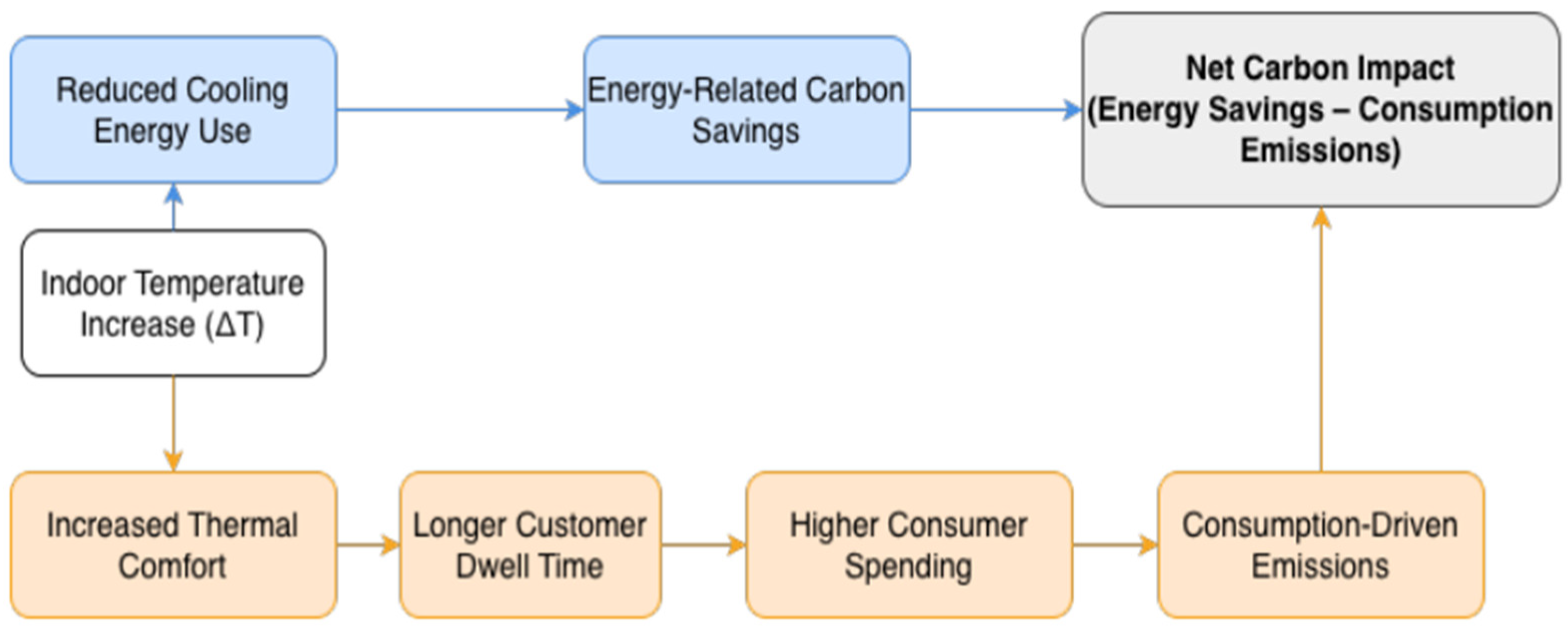
To address these questions, the study develops a dual-pathway carbon accounting framework that integrates operational energy savings with behavior-driven consumption emissions, as illustrated in Figure 1. The following section reviews the theoretical foundations of energy efficiency, thermal comfort, and rebound effects that support this framework.

The framework shows the two pathways through which indoor temperature adjustments may influence carbon outcomes in mercantile buildings. The upper pathway represents the direct operational mechanism, where higher temperature setpoints reduce cooling energy use and generate energy-related carbon savings. The lower pathway captures the indirect behavioral mechanism, where improved thermal comfort may extend customer dwell time, increase spending, and lead to consumption-driven emissions. The overall net carbon impact is determined by the balance between these two opposing effects.

2. Literature Review

2.1. Energy Consumption in Mercantile Buildings

Large commercial spaces, such as mercantile establishments, are highly energy-intensive due to their continuous climate control requirements, high customer traffic, extended operating hours, and large floor areas [6,7]. These characteristics position HVAC systems as a dominant driver of electricity consumption, particularly during summer months when cooling demand peaks. Residential buildings represent a major contributor to energy-sector emissions, accounting for approximately 12.5% of total emissions, primarily due to electricity consumption and fossil fuel use for household activities [31]. As a result, energy policies have traditionally focused on the residential sector, where significant energy-saving potential exists. However, the implementation of energy efficiency measures is often more feasible in non-residential buildings, where operational conditions and centralized management structures provide greater opportunities for intervention [32].

Previous research indicates that a 1 °C increase in the cooling setpoint may reduce total building energy consumption by approximately 1.1%, a relationship that can be cautiously extended to mercantile environments such as shopping malls [33]. Consistent with these findings, other studies report that a 1 °C increase in the cooling setpoint may result in approximately a 6% reduction in cooling energy demand, corresponding to about a 1% decrease in total building energy consumption [34]. While these studies collectively establish a basis for projecting operational carbon savings associated with setpoint increases, they do not account for the behavioral adjustments that may arise in response to altered indoor thermal conditions.

Despite this evidence, most existing frameworks still focus on direct energy savings and rarely incorporate the behavioral and economic responses that may accompany thermal adjustments. Although prior optimization frameworks have effectively prioritized retrofit decisions in commercial buildings by jointly considering investment cost, energy savings, and carbon reductions [35], engineering-based operational analyses typically fail to capture behavioral and consumption-driven sources of emissions. This gap is particularly important in mercantile environments, where customer behavior can directly affect both spending patterns and their related environmental impacts.

2.2. Temperature and Its Effects on Human Behavior

Thermal comfort is closely linked to the human body’s ability to maintain a stable internal temperature despite changes in the surrounding environment. The human thermoregulation system works to keep core body temperature near 37 °C through physiological and behavioral adaptation mechanisms, including changes in metabolic rate, clothing insulation, and interaction with the environment [36,37]. Accordingly, thermal comfort is not determined only by environmental conditions, but also by individuals’ adaptive capacity. ASHRAE defines thermal comfort as a psychological state reflecting satisfaction with the surrounding thermal environment [38]. Since conventional indoor setpoints in commercial buildings are often maintained around 23 °C, while occupants under typical summer conditions in the United States, where daytime outdoor temperatures are around 30 °C, may prefer indoor temperatures closer to 26 °C, moderate setpoint increases may move conditions toward, rather than away from, occupant comfort preferences [9,10,39].

Temperature also influences human perception, cognition, and behavior. Previous research distinguishes between thermal sensation and thermal satisfaction, showing that comfort depends partly on the ability to adapt to environmental conditions [40]. Thermal comfort assessment has therefore expanded from purely environmental variables to broader frameworks that include personal factors such as activity level and clothing insulation, as reflected in indices such as PMV, PET, UTCI, and COMFA [41]. Beyond physiological comfort, temperature can shape psychological and economic responses. For example, physical sensations of coldness have been shown to influence attitudes toward emotionally cold advertisements, while ambient temperature in commercial settings has been linked to perceptions of quality, bidding behavior, and negotiation strategies [42,43,44,45].

In mercantile environments, these behavioral effects are particularly important because indoor conditions can influence how long consumers remain in a store. Prior studies indicate that environmental conditions affect dwell time, which is closely linked to purchasing behavior and revenue generation [17,18]. Improved indoor comfort may encourage longer stays and higher spending, thereby creating a pathway from thermal conditions to consumption-related emissions. Evidence further suggests that even small changes in dwell time can produce notable changes in expenditure, with elasticity estimates typically ranging from 0.6 to 1.3 [17,19]. From a broader perspective, these findings imply that the carbon implications of indoor temperature adjustments extend beyond building operations to include behaviorally mediated consumption effects.

2.3. Jevons Paradox and Behavioral Rebound Effects

In general, energy efficiency improvements and related policy interventions are expected to reduce overall energy consumption [46]. However, behavioral and economic responses can reduce, offset, or even reverse the expected savings over time [26]. This mechanism is commonly described as the rebound effect or Jevons paradox, where efficiency improvements lower the effective cost of an energy service and may encourage additional consumption [47]. Prior studies distinguish between direct rebound, where efficiency gains increase the use of the same energy service, and indirect rebound, where cost savings or behavioral responses increase the consumption of other goods and services with embodied emissions [48,49,50]. Although this may seem counterintuitive, it is now widely recognized that efficiency improvements do not always translate into proportional reductions in total energy use, especially when broader economic feedbacks are considered [24,50,51]. A commonly cited example is aviation, where improvements in fuel efficiency can contribute to lower ticket prices and, in turn, higher demand for air travel [25]. More broadly, rebound effects may also emerge when behavioral responses increase consumption in other domains, generating additional embodied emissions through supply chains [48,49,52].

In mercantile settings, temperature control creates a similar trade-off. Increasing indoor temperature setpoints may reduce cooling-related energy demand, but it may also alter customer experience, dwell time, and spending behavior. If improved thermal comfort leads to greater economic activity, the resulting consumption-driven emissions may offset the operational carbon savings. This creates a plausible behavioral rebound pathway that should be considered when evaluating temperature-based energy efficiency measures in retail environments.

3. Methodology and Analytical Framework

This study develops a quantitative carbon accounting framework to evaluate the net climate impact of increasing indoor temperature setpoints in U.S. mercantile buildings. The framework integrates two analytically distinct emission pathways: (i) operational energy savings resulting from reduced cooling demand and (ii) indirect consumption-driven emissions arising from behaviorally mediated increases in customer spending. The summer season (June–August) is used as the analytical boundary because cooling loads dominate electricity use during this period, while heating demand is negligible.

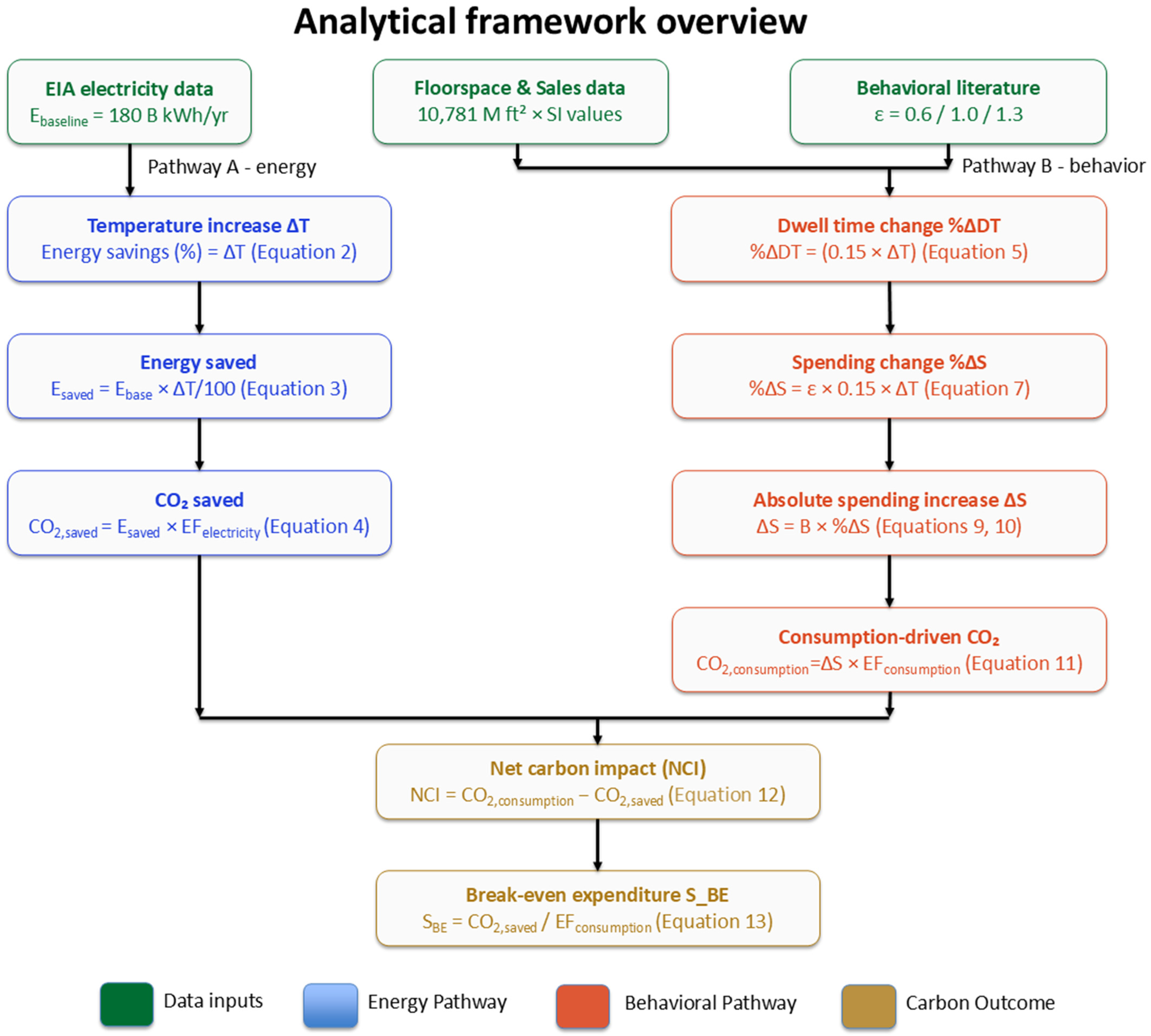
As illustrated in Figure 2, the first pathway quantifies operational energy savings by translating baseline electricity consumption into carbon reductions using a sector-level emission factor (Equations (2)–(4)). The second pathway captures behavioral responses to improved thermal comfort by linking temperature-induced increases in dwell time to changes in consumer spending through an elasticity-based approach and then converting the resulting expenditure into emissions using the EPA USEEIO retail trade emission factor (Equations (5)–(11)). These pathways are combined in a net carbon impact calculation (Equation (12)), which determines whether operational savings are sufficient to offset consumption-driven emissions. A complementary break-even analysis (Equation (13)) identifies the minimum increase in consumer expenditure required to negate operational carbon savings.

All analyses are conducted across discrete scenarios of temperature increase (1–3 °C) and behavioral elasticity (ε = 0.6, 1.0, 1.3), with an additional sensitivity analysis performed over the full continuous parameter space to assess the robustness of the results.

The framework estimates the net carbon impact of indoor temperature setpoint increases through two pathways. The left branch, Pathway A, represents operational energy savings by tracing baseline electricity consumption to carbon reductions using a sector-level emission factor. The right branch, Pathway B, captures the behavioral rebound pathway by linking temperature-induced increases in dwell time to changes in consumer spending through an elasticity parameter (ε = 0.6, 1.0, 1.3) and converting the resulting expenditure into consumption-driven emissions using the EPA USEEIO v1.3 retail-sector emission factor, used here as a mercantile retail proxy. The two pathways converge in the net carbon impact calculation (Equation (12)) and the complementary break-even expenditure threshold (Equation (13)). Numbers in brackets refer to the corresponding equations presented in Section 3.

3.1. Baseline Energy Consumption

The latest CBECS consumption table provides the most recent mercantile-specific electricity consumption estimate [29]. To better reflect recent electricity demand, this value was updated using the change in U.S. commercial sector electricity sales between 2018 and 2024, as reported by EIA [53]. Commercial electricity sales increased from 1,381,755 thousand MWh in 2018 to 1,450,941 thousand MWh in 2024, corresponding to an adjustment factor of 1.05. Accordingly, baseline annual mercantile electricity consumption was updated from 180 billion kWh/year to approximately 189 billion kWh/year. Based on the U.S. EIA’s monthly commercial-sector electricity sales data [53], June–August accounted for approximately 28.1% of annual commercial-sector electricity sales in 2024. A seasonal electricity adjustment factor of 0.281 was therefore applied to convert annual mercantile electricity consumption into a summer-period estimate. Using the updated annual estimate of 189 billion kWh/year, electricity consumption for the June–August cooling season was estimated at 53.1 billion kWh. This value was used as the baseline electricity consumption for the summer-only energy savings analysis. The baseline summer season electricity consumption for the U.S. mercantile building sector was defined as follows:

$${\mathrm{E}}_{\mathrm{b}\mathrm{a}\mathrm{s}\mathrm{e}\mathrm{l}\mathrm{i}\mathrm{n}\mathrm{e}}=53.1 \mathrm{b}\mathrm{i}\mathrm{l}\mathrm{l}\mathrm{i}\mathrm{o}\mathrm{n} \mathrm{k}\mathrm{W}\mathrm{h}$$

(1)

This value represents total electricity consumption across all mercantile building types primarily engaged in retail activities, including both mall and non-mall formats.

3.2. Energy Savings from Temperature Setpoint Increases

Drawing on empirical evidence indicating that each 1 °C increase in the cooling setpoint reduces total building energy consumption by approximately 1–1.1% [33,34], this study adopts a conservative and uniform savings rate of 1% per degree Celsius. For a temperature increase of ΔT (°C), the fractional energy savings can be expressed as:

$$\Delta \mathrm{E}\left(\%\right)=\mathrm{s}\times \Delta \mathrm{T} (\mathrm{s}=1\% \mathrm{per} °\mathrm{C})$$

(2)

The absolute energy saved is then calculated as:

$${\mathrm{E}}_{\mathrm{s}\mathrm{a}\mathrm{v}\mathrm{e}\mathrm{d}}={\mathrm{E}}_{\mathrm{b}\mathrm{a}\mathrm{s}\mathrm{e}\mathrm{l}\mathrm{i}\mathrm{n}\mathrm{e}}\times \left(\Delta \mathrm{T}/100\right)$$

(3)

Carbon savings associated with reduced electricity consumption were estimated by applying an electricity emission factor, EF_electricity, expressed in kg CO₂-eq per kWh:

$${\mathrm{C}\mathrm{O}}_{2,\mathrm{s}\mathrm{a}\mathrm{v}\mathrm{e}\mathrm{d}}={\mathrm{E}}_{\mathrm{s}\mathrm{a}\mathrm{v}\mathrm{e}\mathrm{d}}\times \mathrm{E}{\mathrm{F}}_{\mathrm{e}\mathrm{l}\mathrm{e}\mathrm{c}\mathrm{t}\mathrm{r}\mathrm{i}\mathrm{c}\mathrm{i}\mathrm{t}\mathrm{y}}$$

(4)

The electricity emission factor was set to 0.4 kg CO₂/kWh. This value is consistent with the EPA [54] national average delivered electricity emission rate, which accounts for transmission and distribution losses and is approximately 0.394 kg CO₂/kWh. The value was rounded to 0.4 kg CO₂/kWh for scenario-based calculations.

An operational (delivered-electricity) emission factor is used here, whereas consumption-driven emissions are estimated using a life-cycle factor spanning the supply chain (Section 3.5). This difference reflects a consequential perspective that traces the marginal downstream emissions induced by an operational decision rather than a single attributional inventory, consistent with the indirect-rebound literature [48,49,52]. The robustness of this boundary choice is examined in Section 4.6.5.

Thermal comfort at the adopted 26 °C cooling setpoint was verified for active mercantile occupants using the CBE Thermal Comfort Tool [55]. Unlike sedentary office environments (~1.2 met), mercantile settings involve light walking activity (~1.6 met) [11]. Although a higher metabolic rate generally lowers the thermal neutral temperature, with recent evidence suggesting a reduction of approximately 0.3 °C for every 0.1 met increase in activity level [22], walking also raises the relative air speed and dynamically reduces the effective clothing insulation to 0.42 clo, partially offsetting the additional metabolic heat production. For 1.6 met, 0.42 clo, and a relative air speed of approximately 0.38 m/s (resulting from light walking at a still-air value of 0.2 m/s), the predicted mean vote remained close to neutrality across 40–60% relative humidity (PMV = 0.02 at 40% RH and 0.16 at 60% RH; PPD = 5.0–5.5%; SET = 25.5–26.4 °C), well within the ±0.5 PMV acceptability limit.

3.3. Behavioral Model: Dwell Time and Spending Response

A baseline indoor temperature of 23 °C was adopted as a representative comfort-based indoor condition, consistent with thermal comfort guidance and prior evidence indicating thermal neutrality around 23 °C [9,10,11]. The behavioral component of the framework is grounded in the relationship between thermal comfort and customer dwell time. Based on prior evidence suggesting that indoor thermal conditions may influence customer staying behavior, this study adopts a conservative 15% increase in dwell time per 1 °C increase in indoor setpoint temperature toward the adaptive comfort optimum under summer conditions [20]. The relative change in dwell time for a temperature increase of ΔT is modeled as follows:

$$\%\Delta \mathrm{D}\mathrm{T}=0.15\times \Delta \mathrm{T}$$

(5)

where 0.15 represents the conservative relative increase in staying time associated with each 1 °C temperature increase. This value is further supported by independent field evidence from Xue et al. [21], who observed that average staying length increased from approximately 17.5 min at around 23 °C to approximately 22.5 min at around 25 °C, corresponding to a sensitivity of roughly 14% per °C. Together, these studies support the use of a 15% per °C estimate as a plausible central scenario value for the behavioral model.

To translate changes in dwell time into consumer spending behavior, a spending–dwell time elasticity parameter, ε, is introduced. This parameter is defined as the proportional change in expenditure associated with a proportional change in time spent in-store. The resulting change in consumer spending is expressed as follows:

$$\%\Delta \mathrm{S}=\mathsf{\epsilon }\times \%\Delta \mathrm{D}\mathrm{T}$$

(6)

Substituting Equation (5) into Equation (6) yields the unified behavioral spending response function:

$$\%\Delta \mathrm{S}=\mathsf{\epsilon }\times 0.15\times \Delta \mathrm{T}$$

(7)

Three elasticity scenarios were considered to reflect uncertainty in the strength of the relationship between additional dwell time and consumer expenditure. A lower-response scenario (ε = 0.6) was adopted from the estimate reported by Wu et al. [17], whereas a higher-response scenario (ε = 1.3) was based on evidence summarized by ICSC, citing a study by MIT showing that a 1% increase in dwell time corresponded to an approximately 1.3% increase in sales [19]. The intermediate case (ε = 1.0) was introduced as a unit-elasticity benchmark representing proportional changes in spending and dwell time. Accordingly, the three values span conservative, moderate, and high behavioral responses rather than representing precise estimates for specific retail formats. This discrete scenario analysis is complemented by the Monte Carlo framework (Section 3.8), which continuously samples elasticity values over the range ε = 0.6–1.3.

3.4. Estimation of Baseline Mercantile Sector Expenditure

Total sector-level expenditure was estimated using a floorspace-weighted sales intensity approach. Following the CBECS classification [29]: the total U.S. mercantile building stock was disaggregated into two primary subcategories: non-mall retail (A₁ = 482.45 million m²) and enclosed and strip malls (A₂ = 519.14 million m²), yielding a total floor area of 1001.59 million m², or 10,781 million ft². Category-specific sales intensity (SI) values were assigned based on prevailing retail format characteristics and U.S. Census Bureau [56] estimates. Non-mall retail was represented by a department store proxy (SI₁ = 458 USD/m²), while mall-based retail was approximated using general merchandise sales intensity (SI₂ = 1305 USD/m²).

The baseline total sector expenditure (B) was then computed as follows:

$$\mathrm{B}=\mathrm{A}1\times \mathrm{S}\mathrm{I}1+\mathrm{A}2\times \mathrm{S}\mathrm{I}2$$

(8)

This calculation yielded an estimated annual baseline expenditure of approximately 898.4 billion USD/year for the U.S. mercantile building stock. Because monthly expenditure data are not reported separately for CBECS-defined mercantile buildings, a mercantile-like retail proxy was constructed using U.S. Census Bureau [57] monthly retail trade categories most closely aligned with mercantile retail environments. Not seasonally adjusted monthly sales values were used to preserve seasonal variation. The summer expenditure adjustment factor was calculated as the ratio of June–August sales to annual sales across the selected retail categories. In 2024, the selected mercantile categories accounted for USD 553.8 billion in sales during the June–August period, compared with total annual sales of USD 2179.6 billion, resulting in a summer expenditure adjustment factor of 0.254. Applying this factor to the annual baseline expenditure estimate of 898.4 billion USD/year resulted in a summer-period baseline expenditure of approximately 228.3 billion USD. This value was used as the baseline expenditure for estimating behavior-induced spending increases during the summer cooling season.

Category-level differentiation is applied only on the expenditure side, where format-specific sales-intensity data are available (Section 3.4). By contrast, energy consumption is represented by a sector-level baseline that already aggregates both non-mall retail and enclosed/strip-mall formats [29]. Likewise, operational savings rates and behavioral parameters are modeled uniformly, as reliable format-specific estimates are not currently available at comparable resolution. Moreover, any category-specific differences would affect both the operational-savings and consumption pathways, suggesting that their omission is unlikely to alter the qualitative comparison between the two. Accordingly, the present analysis should be interpreted as a sector-level assessment rather than a comparison among retail subcategories. Sensitivity and Monte Carlo analyses (Section 3.8 and Section 4.6) further indicate that the principal conclusions are robust to wide variations in these parameters.

3.5. Consumption-Driven Emissions

The absolute increase in consumer expenditure driven by behavioral responses to temperature change is given by:

$$\Delta \mathrm{S}=\mathrm{B}\times \%\Delta \mathrm{S}$$

(9)

Substituting Equations (7) and (8) into Equation (9):

$$\Delta \mathrm{S}=\mathrm{B}\times \mathsf{\epsilon }\times 0.15\times \Delta \mathrm{T}$$

(10)

Consumption-driven CO₂ emissions were estimated by applying the EPA USEEIO v1.3 emission factor for retail trade (EF_consumption = 0.164 kg CO₂-eq per USD) [30].

$${\mathrm{C}\mathrm{O}}_{2,\mathrm{c}\mathrm{o}\mathrm{n}\mathrm{s}\mathrm{u}\mathrm{m}\mathrm{p}\mathrm{t}\mathrm{i}\mathrm{o}\mathrm{n}}=\Delta \mathrm{S}\times \mathrm{E}{\mathrm{F}}_{\mathrm{c}\mathrm{o}\mathrm{n}\mathrm{s}\mathrm{u}\mathrm{m}\mathrm{p}\mathrm{t}\mathrm{i}\mathrm{o}\mathrm{n}}$$

(11)

3.6. Net Carbon Impact and Break-Even Analysis

The net carbon impact (NCI) associated with a given temperature increase scenario was calculated as the difference between consumption-driven emissions and operational carbon savings:

$$\mathrm{N}\mathrm{C}\mathrm{I}=\mathrm{C}{\mathrm{O}}_{2,\mathrm{c}\mathrm{o}\mathrm{n}\mathrm{s}\mathrm{u}\mathrm{m}\mathrm{p}\mathrm{t}\mathrm{i}\mathrm{o}\mathrm{n}}-\mathrm{C}{\mathrm{O}}_{2,\mathrm{s}\mathrm{a}\mathrm{v}\mathrm{e}\mathrm{d}}$$

(12)

A positive NCI indicates that behavioral rebound emissions outweigh direct operational savings, resulting in an overall increase in carbon emissions. In contrast, an NCI value of zero or lower indicates carbon neutrality or a net reduction in emissions. To identify the minimum level of additional spending required to offset operational carbon savings, the break-even expenditure, ${\mathrm{S}}_{\mathrm{B}\mathrm{E}}$, was obtained by setting Equation (12) equal to zero and solving for $\Delta \mathrm{S}$:

$${\mathrm{S}}_{\mathrm{B}\mathrm{E}}=\mathrm{C}{\mathrm{O}}_{2,\mathrm{s}\mathrm{a}\mathrm{v}\mathrm{e}\mathrm{d}}/\mathrm{E}{\mathrm{F}}_{\mathrm{c}\mathrm{o}\mathrm{n}\mathrm{s}\mathrm{u}\mathrm{m}\mathrm{p}\mathrm{t}\mathrm{i}\mathrm{o}\mathrm{n}}$$

(13)

Expressed in billion USD, this threshold represents the minimum additional consumer spending needed to fully offset the carbon benefits associated with a given temperature setpoint increase, regardless of the assumed elasticity scenario.

3.7. Sensitivity Analysis

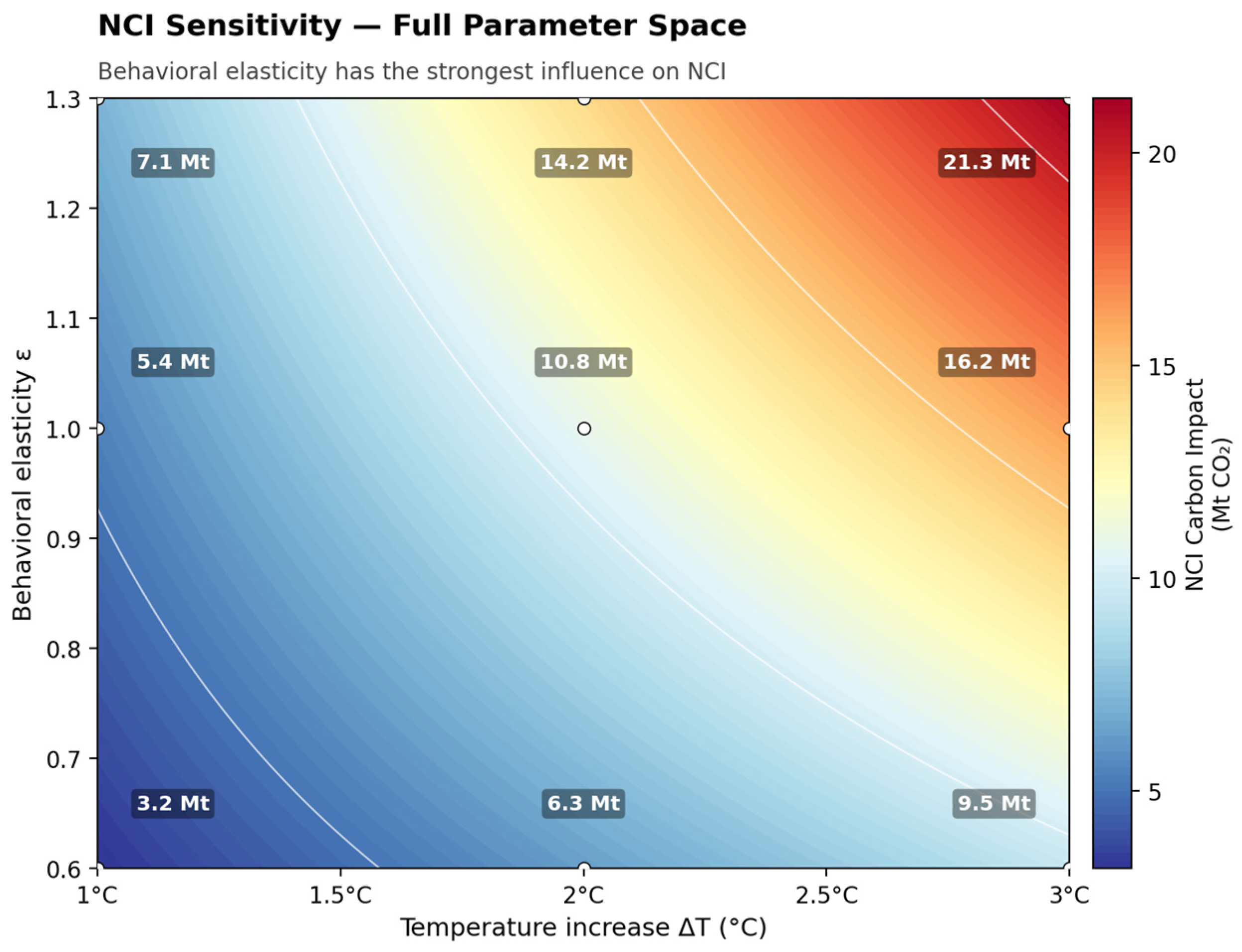
The sensitivity analysis was implemented as a deterministic two-dimensional grid evaluation. The net carbon impact (Equations (3)–(12)) was computed at each point of a regular grid over the two principal scenario variables, temperature increase (ΔT ∈ [1, 3] °C) and behavioral elasticity (ε ∈ [0.6, 1.3]), while the remaining parameters were fixed at their central values (s = 1% per °C, d = 15% per °C, EF_electricity = 0.40 kg CO₂/kWh, and EF_consumption = 0.164 kg CO₂/USD). These two variables were selected because they constitute the primary scenario dimensions of the study and directly represent the operational intervention (temperature increase) and the behavioral response mechanism (spending elasticity). The resulting analysis generated a continuous response surface describing how net carbon impact varies across the principal scenario space and enabled identification of any carbon-neutral or net-reduction region within the modeled range. The resulting response surface is presented in Figure 3.

Unlike the Monte Carlo analysis presented in Section 3.8, which propagates uncertainty simultaneously across six parameters, the deterministic sensitivity analysis was not intended as a comprehensive uncertainty assessment. Rather, its purpose was to isolate and visualize the influence of the two principal scenario variables while holding all other assumptions constant. Accordingly, Section 3.7 provides parameter-level insight into the structure of the rebound mechanism, whereas Section 3.8 evaluates the robustness of the findings under simultaneous uncertainty in behavioral, climatic, structural, and emissions-related parameters across the broader model.

3.8. Monte Carlo Uncertainty Analysis

To further evaluate the robustness of the deterministic sensitivity results, a Monte Carlo uncertainty analysis with 10,000 iterations was conducted in R using a fixed random seed for reproducibility. Whereas the deterministic sensitivity analysis in Section 3.7 focused on the isolated effects of the two principal scenario variables, temperature increase (ΔT) and behavioral elasticity (ε), the Monte Carlo framework propagated uncertainty simultaneously across all uncertain model parameters. The objective was to determine whether the dominance of consumption-driven emissions remained under joint parameter uncertainty rather than under individual parameter variations alone.

In each iteration, six uncertain input parameters (ΔT, ε, s, d, EF_electricity, and EF_consumption) were randomly and independently sampled from predefined ranges based on the scenario analysis and the relevant literature. Uniform distributions were used for all uncertain parameters; in the absence of empirical information regarding their underlying probability distributions, uniform distributions provide a conservative and transparent representation of uncertainty [58]. Temperature increase (ΔT) was sampled between 1 and 3 °C, and behavioral elasticity (ε) between 0.6 and 1.3. The dwell-time response parameter (d) was varied between 10% and 20% per °C to reflect uncertainty around the central estimate of 15% per °C. The electricity emission factor (EF_electricity) was sampled between 0.35 and 0.45 kg CO₂/kWh, whereas the consumption emission factor (EF_consumption) was sampled between 0.13 and 0.20 kg CO₂/USD. Baseline summer electricity consumption and baseline summer expenditure were held constant at 53.1 billion kWh and 228.3 billion USD, respectively.

Special attention was given to the energy-savings coefficient (s), since cooling-energy savings can vary substantially across climate zones, humidity conditions, HVAC performance, building-envelope quality, infiltration rates, and operational characteristics [59]. To capture this variability, the energy-savings coefficient was sampled between 0.9% and 5.5% per °C (0.009–0.055). This range was derived from climate-specific cooling-setpoint simulations reported by Ghahramani et al. [59] and was conservatively translated from HVAC-level savings to whole-building electricity impacts, recognizing that HVAC systems account for approximately 43% of commercial-building electricity consumption [59]. The selected range encompasses the deterministic value of 1% per °C while allowing for both lower and substantially higher savings under different climatic and building conditions. These parameters and their sampling ranges are summarized in

Table 1. Input parameters and distributions used in the Monte Carlo uncertainty analysis.

Parameter	Symbol	Distribution	Range/Value	Unit
Baseline summer electricity consumption	Ebase	Fixed	53.1 × 109	kWh
Baseline summer expenditure	Bbase	Fixed	228.3 × 109	USD
Temperature increase	ΔT	Uniform	1–3	°C
Behavioral elasticity	ε	Uniform	0.6–1.3	Dimensionless
Energy savings rate	s	Uniform	0.009–0.055	per °C
Dwell-time response	d	Uniform	0.10–0.20	per °C
Electricity emission factor	EFelectricity	Uniform	0.35–0.45	kg CO2/kWh
Consumption emission factor	EFconsumption	Uniform	0.13–0.20	kg CO2/USD
Number of simulations	n	Fixed	10,000	Iterations

.

For each simulation, operational carbon savings, consumption-driven emissions, the consumption-to-savings ratio, break-even expenditure, and net carbon impact were recalculated using the framework described in Section 3.2, Section 3.3, Section 3.4, Section 3.5 and Section 3.6. Results were summarized using the mean, median, minimum and maximum values, 95% uncertainty intervals, and the probability of a positive net carbon impact. This probability was defined as the proportion of simulations in which consumption-driven emissions exceeded operational carbon savings and was used as an indicator of the robustness of the rebound-dominance finding under simultaneous parameter uncertainty. The results of the Monte Carlo analysis are presented in Section 4.6.6.

3.9. Robustness Analysis Under Behavioral Heterogeneity

To further evaluate the robustness of the sign of the net carbon impact, two complementary threshold conditions were derived by setting Equation (12) equal to zero. These thresholds are not intended as empirical estimates, but rather as robustness bounds indicating how much the behavioral response would have to weaken before operational carbon savings exceed consumption-driven emissions.

First, solving Equation (12) for the combined behavioral response yields the critical behavioral product:

$${\left(\mathrm{\epsilon }\times \mathrm{d}\right)}_{\mathrm{c}\mathrm{r}\mathrm{i}\mathrm{t}}={\displaystyle \frac{{\mathrm{E}}_{\mathrm{b}\mathrm{a}\mathrm{s}\mathrm{e}\mathrm{l}\mathrm{i}\mathrm{n}\mathrm{e}}\times \mathrm{s}\times \mathrm{E}{\mathrm{F}}_{\mathrm{e}\mathrm{l}\mathrm{e}\mathrm{c}\mathrm{t}\mathrm{r}\mathrm{i}\mathrm{c}\mathrm{i}\mathrm{t}\mathrm{y}}}{\mathrm{B}\times \mathrm{E}{\mathrm{F}}_{\mathrm{c}\mathrm{o}\mathrm{n}\mathrm{s}\mathrm{u}\mathrm{m}\mathrm{p}\mathrm{t}\mathrm{i}\mathrm{o}\mathrm{n}}}}$$

(14)

where d denotes the proportional increase in dwell time per °C and ε represents the spending elasticity with respect to dwell time. Values above this threshold imply that consumption-driven emissions exceed operational carbon savings, resulting in a positive net carbon impact.

Second, to account for behavioral heterogeneity and the possibility that only a fraction of the modeled spending response is effectively active, an active participation share φ ∈ [0, 1] was introduced. The parameter φ represents the effective portion of the modeled spending response that remains behaviorally active after accounting for heterogeneity, spending displacement, and segment-specific differences in consumer reactions. Solving Equation (12) for the critical participation share yields:

$${\mathrm{\phi }}^{*}={\displaystyle \frac{\mathrm{C}{\mathrm{O}}_{2,\mathrm{s}\mathrm{a}\mathrm{v}\mathrm{e}\mathrm{d}}}{\mathrm{C}{\mathrm{O}}_{2,\mathrm{c}\mathrm{o}\mathrm{n}\mathrm{s}\mathrm{u}\mathrm{m}\mathrm{p}\mathrm{t}\mathrm{i}\mathrm{o}\mathrm{n}}}}={\displaystyle \frac{{\mathrm{E}}_{\mathrm{b}\mathrm{a}\mathrm{s}\mathrm{e}\mathrm{l}\mathrm{i}\mathrm{n}\mathrm{e}}\times \mathrm{s}\times \mathrm{E}{\mathrm{F}}_{\mathrm{e}\mathrm{l}\mathrm{e}\mathrm{c}\mathrm{t}\mathrm{r}\mathrm{i}\mathrm{c}\mathrm{i}\mathrm{t}\mathrm{y}}}{\mathrm{B}\times \mathsf{\epsilon }\times \mathrm{d}\times \mathrm{E}{\mathrm{F}}_{\mathrm{c}\mathrm{o}\mathrm{n}\mathrm{s}\mathrm{u}\mathrm{m}\mathrm{p}\mathrm{t}\mathrm{i}\mathrm{o}\mathrm{n}}}}$$

(15)

Whenever the active share φ exceeds the critical value φ*, consumption-driven emissions outweigh operational carbon savings. Values below φ* imply that operational carbon savings exceed consumption-driven emissions.

Together, these threshold conditions quantify how far the behavioral pathway would need to weaken for the net carbon impact to become neutral or negative. They therefore provide robustness bounds rather than empirical estimates and complement the uncertainty analysis described in Section 3.8. Their numerical implications are presented in Section 4.6.1 and Section 4.6.2.

3.10. Non-Linear Comfort Specification

To relax the assumption of a uniformly positive linear dwell-time response, the comfort-driven dwell-time function was alternatively specified as an inverted-U (parabolic) curve, consistent with the established finding that thermal comfort is maximized at an optimal temperature and declines on either side of it. This relationship corresponds to the inverse of the U-shaped Predicted Percentage Dissatisfied (PPD) curve in Fanger’s thermal comfort model [38,60].

The relative dwell-time gain was modeled as a quadratic function peaking at the comfort optimum (T* = 26 °C), corresponding to ΔT* = 3 °C above the 23 °C baseline and reflecting the thermally neutral condition verified for active mercantile occupants in Section 3.2:

$$\%\Delta \mathrm{D}\mathrm{T}\left(\Delta \mathrm{T}\right)=\%\Delta \mathrm{D}{\mathrm{T}}_{\mathrm{m}\mathrm{a}\mathrm{x}}\left[1-{\left({\displaystyle \frac{\Delta \mathrm{T}-\Delta {\mathrm{T}}^{*}}{\Delta {\mathrm{T}}^{*}}}\right)}^2\right]$$

(16)

where %ΔDT_max was calibrated so that the initial slope around the 23 °C baseline reproduces the central estimate of 15% per °C used in the linear specification, yielding %ΔDT_max = 22.5%. This formulation preserves comparability with the linear model near the baseline while allowing marginal dwell-time gains to diminish progressively as conditions approach the comfort optimum and to decline beyond it. By construction, the function yields zero dwell-time gain at the 23 °C baseline and reaches its maximum at the comfort optimum of 26 °C.

Within the policy-relevant range considered in this study (ΔT ≤ 3 °C), the specification captures the concave, diminishing-returns portion of the inverted-U relationship. Net carbon impact was then recomputed using Equations (6)–(12), with the dwell-time response from Equation (16) replacing the linear term. The resulting estimates were compared with those obtained under the baseline linear specification to evaluate the sensitivity of the findings to nonlinear thermal-comfort dynamics. Results are presented in Section 4.6.3.

3.11. Diminishing-Returns Spending Specification

To account for diminishing marginal returns to additional time spent in-store, consumer spending was alternatively modeled using a saturating response function:

$$\%\Delta \mathrm{S}={\displaystyle \frac{\mathsf{\epsilon }}{\mathrm{k}}}\left(1-{\mathrm{e}}^{-\mathrm{k}\Delta \mathrm{D}\mathrm{T}}\right)$$

(17)

where k governs the rate of saturation and %ΔDT is the relative change in dwell time defined in Equation (5). This specification was chosen because it preserves the baseline spending elasticity while allowing marginal spending gains to diminish progressively as dwell time increases. At the baseline condition, it reduces to the linear elasticity form (Equation (6)), while introducing progressively smaller incremental spending responses at higher dwell times. This concave behavior is consistent with the law of diminishing marginal returns and with evidence from environmental psychology indicating that behavioral responses to retail environments are nonlinear, in which store-induced pleasure and arousal are associated with longer dwell times and greater unplanned spending [61,62,63]. The parameter k determines how rapidly saturation occurs. Following the principle of parsimony, k was set to 1, yielding a moderate rate of diminishing returns while preserving comparability with the baseline linear specification. Net carbon impact was then recomputed using Equations (9)–(12), with the spending response from Equation (17) replacing the linear term. Results are presented in Section 4.6.4.

4. Results

This section presents the net carbon impact of increasing indoor temperature setpoints across all simulated scenarios, separating the results into operational carbon savings and consumption-driven emissions. The results directly address the central research question of the study: whether operational energy savings in U.S. mercantile buildings lead to net carbon benefits or are offset by consumption-driven emissions associated with behavioral rebound effects. The analysis begins with scenario-level results (Section 4.1 and Section 4.2), extends to the full parameter space (Section 4.3), examines the relative contributions of the two emissions pathways (Section 4.4), presents the complete results matrix (Section 4.5), and concludes with a series of robustness analyses designed to test the sensitivity of the findings to alternative assumptions and model specifications (Section 4.6).

4.1. Comparative Analysis of Energy Savings and Consumption-Driven Emissions

Indoor temperature adjustments shape carbon outcomes through two channels that work in opposite directions. The first is the direct drop in cooling energy use that comes with a higher setpoint. The second is harder to see in conventional accounting: when thermal conditions improve, customers tend to linger and spend more, and that extra economic activity carries its own embodied emissions. Whether a temperature intervention actually delivers a net carbon benefit depends on how these two channels balance out.

The numbers in our scenarios make the imbalance hard to miss. Operational savings stay in a narrow band of 0.21–0.64 Mt CO₂, while consumption-driven emissions land somewhere between 3.37 and 21.90 Mt CO₂. Even at the conservative end of behavioral response, the consumption side is more than ten times the operational side. Figure 3 maps the resulting net carbon impact (NCI) across the full parameter space defined by ΔT and ε. Behavioral elasticity does most of the work in driving NCI; temperature pushes the result up too, but its effect is more proportional and less steep. The contours steepen visibly as elasticity rises, which is another way of saying that what customers do with the space matters more than how warm we let it get.

Within the modeled range, no setpoint we tested gets close to carbon neutrality. That alone makes the case for bringing behavioral responses into how indoor temperature strategies are evaluated.

4.2. Break-Even Dynamics, Behavioral Risk, and Long-Term Carbon Debt

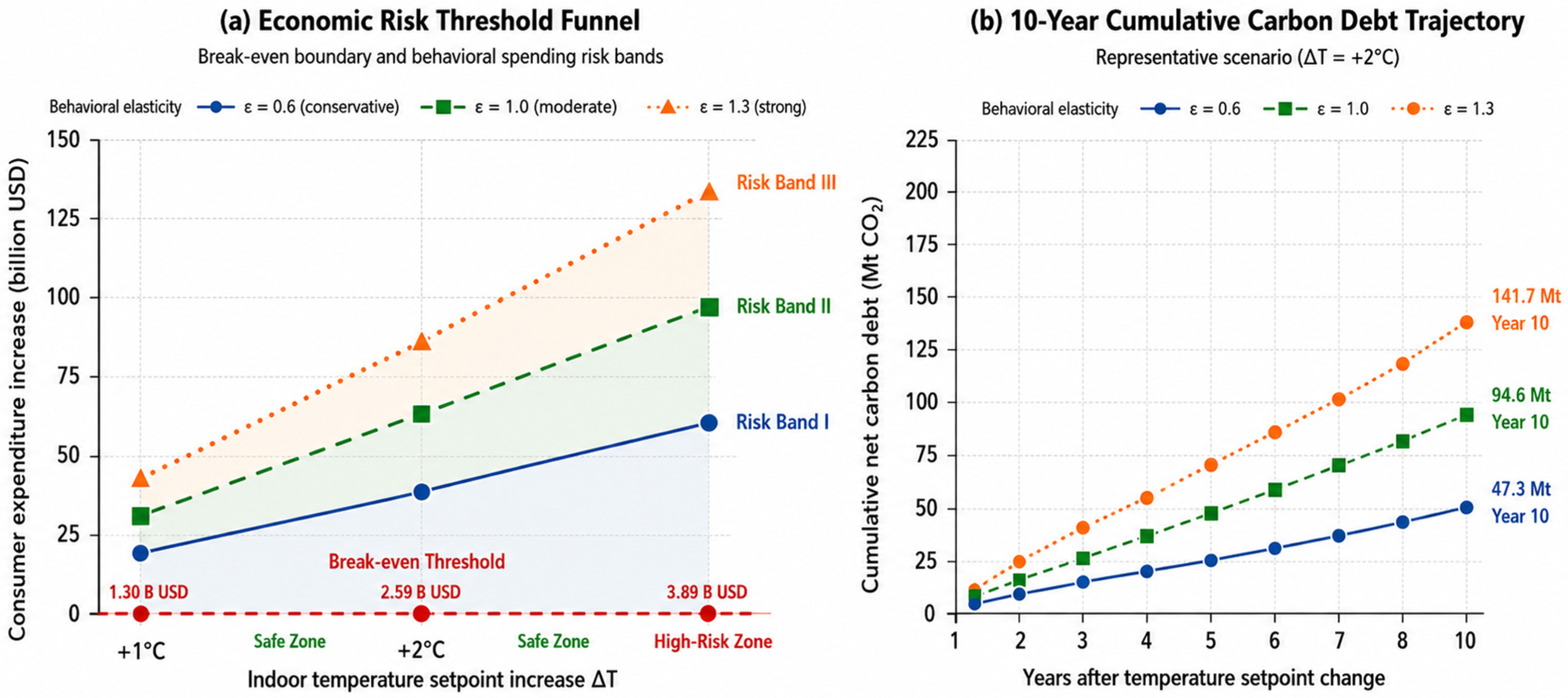
Indoor temperature adjustments shape carbon outcomes through a mix of operational, behavioral, and temporal mechanisms. A higher setpoint cuts cooling electricity demand, but the spending changes that follow can produce extra emissions that eat into those operational gains. To test how robust this trade-off is, Figure 4 looks at two related angles: the economic carbon risk that comes with temperature adjustments, and how carbon debt builds up over a ten-year window.

Figure 4a looks at the economic carbon risk side of indoor temperature adjustments. The break-even boundary marks the minimum spending level at which energy savings get fully offset, and adjacent risk bands group behavioral spending into low, moderate, and high-risk regions. Break-even rises from 1.30 billion USD at 1 °C to 3.89 billion USD at 3 °C roughly 0.57–1.70% of the summer-period baseline expenditure. Behavior-induced spending increases, by comparison, run between 20.54 and 133.53 billion USD, putting every elasticity scenario well past the break-even line.

Figure 4b tracks cumulative carbon debt over ten years for the representative ΔT = 2 °C scenario. Carbon debt stays positive throughout, climbing steadily under every elasticity assumption. By year ten, it reaches roughly 63.1 Mt CO₂ under conservative elasticity, 108.1 Mt CO₂ under moderate, and 141.7 Mt CO₂ under strong. Even on the conservative end, operational energy savings cannot keep pace with the long-term emissions that consumption growth brings with it.

Beyond their effects on short-term carbon outcomes, the results indicate that behavioral rebound effects can accumulate into substantial long-term emissions burdens. As a result, assessments of temperature-based energy efficiency measures that consider only operational energy savings may provide an incomplete account of their overall carbon consequences.

4.3. Sensitivity Analysis of Net Carbon Impact

While earlier sections focused on discrete scenario outcomes, this section opens the analysis up to the full parameter space—looking for underlying patterns, dominant mechanisms, and policy-relevant thresholds.

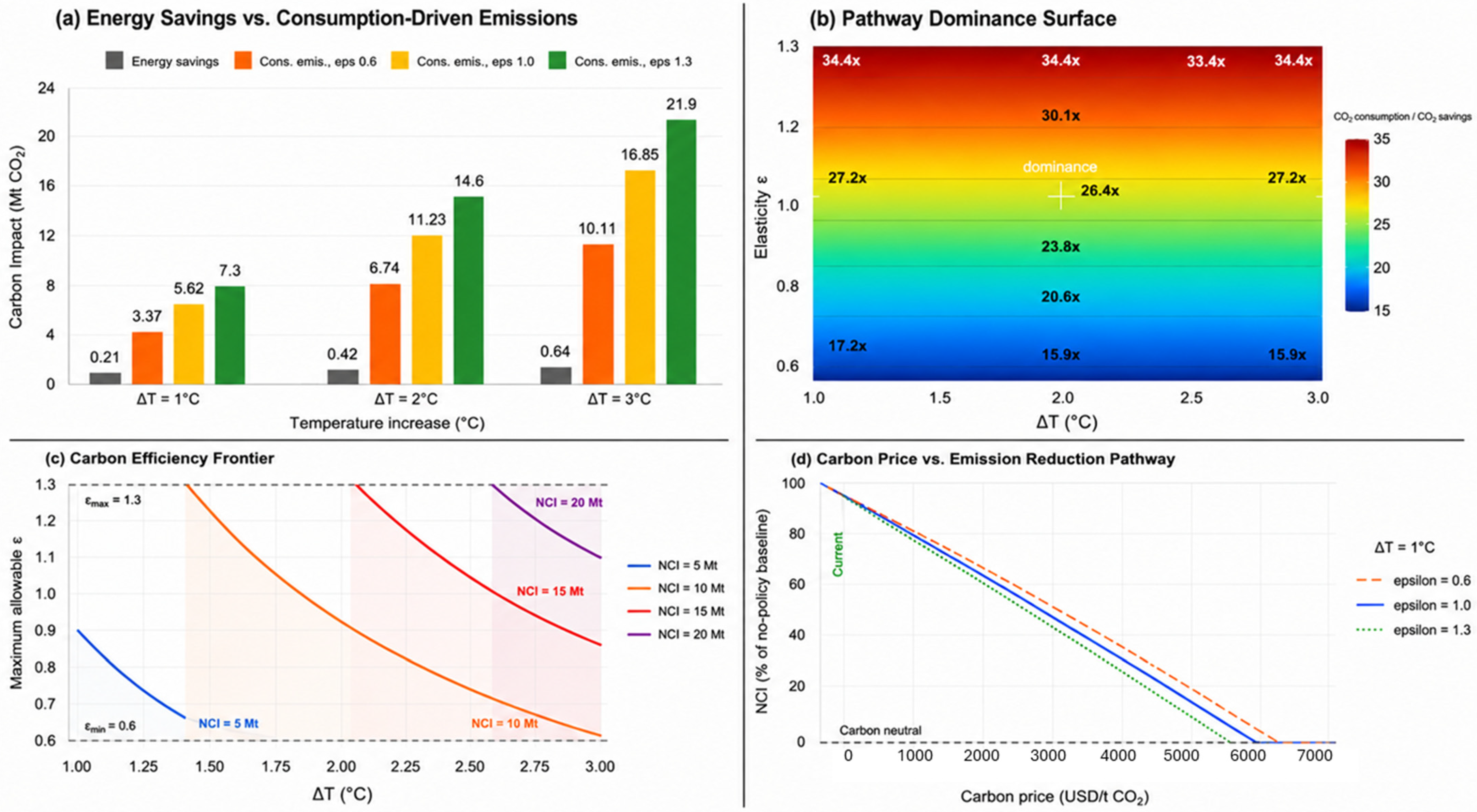
A sensitivity analysis was run across joint variations in temperature increase (ΔT = 1–3 °C) and behavioral elasticity (ε = 0.6–1.3). Results appear in Figure 5, which gives a multi-panel view: discrete outcomes, continuous system dynamics, constraint boundaries, and policy implications.

Figure 5a puts operational energy savings side by side with consumption-driven emissions across the representative scenarios. Energy savings stay small in every case, between 0.21 and 0.64 Mt CO₂, while consumption-driven emissions run from 3.37 to 21.90 Mt CO₂. The net carbon impact comes out positive throughout, with consumption-related emissions outpacing the savings from reduced cooling demand.

Figure 5b extends the picture into a continuous framework with a dominance surface defined by the ratio of consumption-driven emissions to energy savings. Across the entire parameter space, that ratio stays well above one, from roughly 15.9× to 34.4×. No combination of ΔT and ε within the modeled range produces a net emissions reduction. The smooth gradient tells us behavioral elasticity is the strongest hand on the wheel.

Figure 5c presents the carbon efficiency frontier, defined as the maximum elasticity value that maintains NCI below selected threshold levels. The results show that the allowable elasticity decreases as temperature increases, indicating that progressively stronger control of behavioral responses would be required to satisfy more stringent emissions targets. These findings suggest that the effectiveness of temperature-based efficiency measures is inherently constrained when the emissions consequences of behavioral responses are not taken into account.

Figure 5d takes a policy angle by tying net carbon impact to carbon pricing. Achieving carbon neutrality would call for carbon prices in the range of several thousand USD per ton of CO₂ orders of magnitude above where current or realistically anticipated policy lands. Conventional carbon pricing on its own is not going to offset the consumption-driven emissions seen here.

Across the four panels, net carbon impact stays positive throughout the modeled conditions, with behavioral elasticity as the dominant driver. Energy efficiency measures evaluated in isolation are not enough to deliver net emission reductions without explicitly accounting for what happens on the consumption side.

4.4. Carbon Impact Decomposition

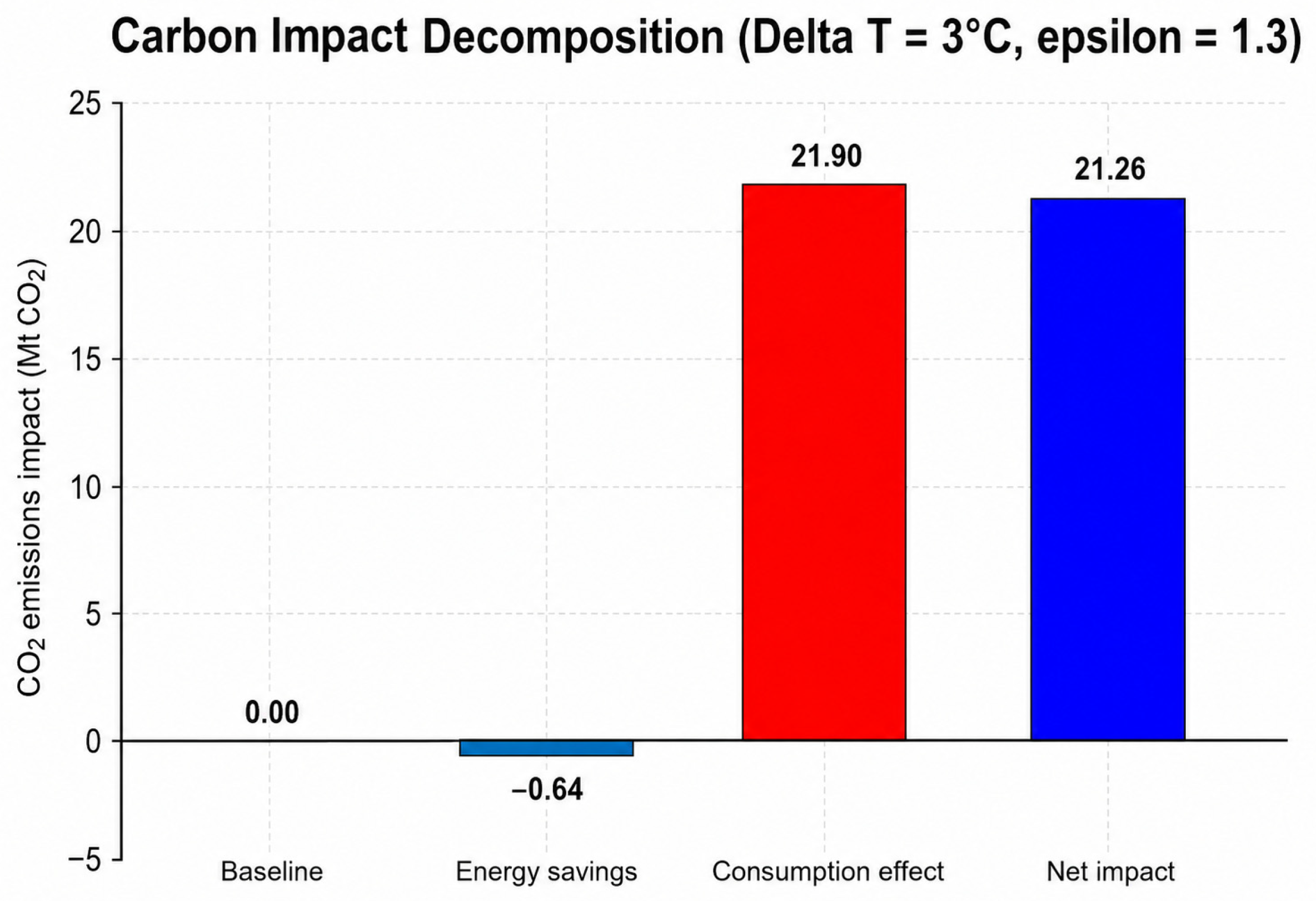
To better illustrate the structural imbalance between operational savings and consumption-driven emissions, a decomposition analysis was conducted for the most extreme scenario considered in this study (ΔT = 3 °C, ε = 1.3), representing the upper bounds of both temperature-induced energy savings and behavioral response within the analyzed parameter range. As Figure 6 shows, energy-related carbon savings reached roughly 0.64 Mt CO₂, while consumption-driven emissions under the same conditions hit 21.90 Mt CO₂, leaving a net carbon impact of about 21.26 Mt CO₂.

The behavioral consumption pathway substantially outweighs the operational energy savings pathway. Even under the maximum temperature adjustment scenario, the reduction in cooling-related emissions stays small next to the additional emissions from increased consumer spending.

Accordingly, the decomposition analysis suggests that net carbon outcomes are dominated by consumption-related effects, while operational energy savings play a comparatively minor mitigating role within the scope of the present analysis.

4.5. Scenario Comparison: Expanded Results Summary

Table 2. Scenario results matrix. The table reports temperature increase (°C), behavioral elasticity (ε), operational energy savings (Mt CO₂), consumption-driven emissions (Mt CO₂), net carbon impact (NCI, Mt CO₂), the consumption-to-savings ratio, and break-even expenditure (billion USD).

Temperature Increase (°C)	Elasticity (ε)	Energy Savings (Mt CO2)	Consumption-Driven Emissions (Mt CO2)	Net Carbon Impact (Mt CO2)	Relative Impact (×Energy Savings)	Break-Even Expenditure (Billion USD)
1	0.6	0.21	3.37	3.16	15.9×	1.30
1	1.0	0.21	5.62	5.40	26.4×	1.30
1	1.3	0.21	7.30	7.09	34.4×	1.30
2	0.6	0.42	6.74	6.31	15.9×	2.59
2	1.0	0.42	11.23	10.81	26.4×	2.59
2	1.3	0.42	14.60	14.17	34.4×	2.59
3	0.6	0.64	10.11	9.47	15.9×	3.89
3	1.0	0.64	16.85	16.21	26.4×	3.89
3	1.3	0.64	21.90	21.26	34.4×	3.89

summarizes the complete results matrix for all nine combinations of temperature increase (1–3 °C) and behavioral elasticity (ε = 0.6, 1.0, 1.3). The table reports operational energy savings, consumption-driven emissions, net carbon impact (NCI), the consumption-to-savings ratio, and the break-even expenditure required to offset operational carbon savings.

The scenario results show that energy savings remain modest throughout the modeled range, varying from 0.21 to 0.64 Mt CO₂. In contrast, consumption-driven emissions range from 3.37 to 21.90 Mt CO₂, resulting in consistently positive net carbon impacts across all scenarios. NCI ranges from 3.16 Mt CO₂ under the most conservative scenario (ΔT = 1 °C, ε = 0.6) to 21.26 Mt CO₂ under the strongest behavioral response scenario (ΔT = 3 °C, ε = 1.3).

The consumption to savings ratio remains well above one in all cases, ranging from 15.9× to 34.4×. Because both behavior-induced spending increases and break-even expenditure scale proportionally with temperature, this ratio remains constant across temperature levels for each elasticity assumption. Break-even expenditure increases linearly with temperature, from 1.30 billion USD at 1 °C to 3.89 billion USD at 3 °C.

Across the range of temperature adjustments and behavioral elasticities evaluated in this study, operational carbon savings were consistently outweighed by consumption-driven emissions. As a result, no scenario within the modeled parameter space yielded a net reduction in carbon emissions under the assumptions adopted in the analysis.

4.6. Robustness Analyses

To assess the robustness of the central finding, a series of complementary robustness analyses was conducted. These analyses examined the sensitivity of the results to behavioral heterogeneity (Section 4.6.1 and Section 4.6.2), nonlinear comfort responses (Section 4.6.3), nonlinear spending responses (Section 4.6.4), accounting-boundary assumptions (Section 4.6.5), and joint parameter uncertainty through the Monte Carlo analysis described in Section 3.8. Together, these analyses evaluate whether the positive net carbon impact persists under alternative behavioral specifications, broader uncertainty ranges, and more comparable carbon-accounting boundaries.

4.6.1. Parameter Sign-Reversal Threshold Analysis

The threshold conditions derived in Section 3.9 were evaluated at the baseline parameter values to quantify how far the behavioral response would need to weaken before the net carbon impact changes sign. Because both operational savings and consumption-driven emissions scale linearly with temperature increase, ΔT cancels from the sign condition, leaving the outcome dependent only on the strength of the behavioral response and the active share of induced spending.

Evaluating the critical behavioral product (Equation (14)) at the baseline values yields a threshold of approximately 0.0057 per °C. The modeled behavioral product ranges from 0.090 to 0.195 per °C, indicating that the modeled values exceed the sign-reversal threshold by a factor of approximately 16 to 34. Equivalently, holding the dwell-time response constant at 15% per °C, the spending elasticity would have to fall below approximately 0.04, compared with the conservative lower-bound value of 0.6. Alternatively, holding the elasticity at 0.6, the dwell-time response would have to fall below approximately 0.95% per °C, compared with the baseline value of 15% per °C.

These results indicate that the sign of the net carbon impact would reverse only if the comfort–dwell-time–spending pathway were substantially weaker than assumed in the baseline analysis. In practical terms, the behavioral response would need to be reduced by approximately one order of magnitude relative to the conservative values adopted in this study before operational carbon savings exceed consumption-driven emissions.

4.6.2. Partial Participation Threshold Analysis

Evaluating the critical participation share (Equation (15)) yields values of 2.9% to 6.3% across the elasticity scenarios. Equivalently, more than 94–97% of the modeled spending response would have to be displaced or behaviorally inactive for operational carbon savings to exceed consumption-driven emissions. These results indicate that the net carbon impact remains positive even when only a small fraction of the modeled spending response is active. Consequently, pronounced heterogeneity across store formats or shopping trips does not alter the aggregate sign, provided the rebound channel remains active in more than a few percent of transactions.

Table 3. Robustness of the net carbon impact sign. For each criterion, the modeled (central) value is compared with the critical value at which net carbon impact equals zero (NCI = 0). The safety margin is defined as the factor by which the modeled value exceeds the critical value and is numerically equivalent to the consumption-to-savings ratio (R) reported in Table 2.

Robustness Criterion	Symbol	Modeled Value	Critical Value (NCI = 0)	Safety Margin
Behavioral product (elasticity × dwell-time response)	ε $\times$ d	0.090–0.195 per °C	≈0.0057 per °C	15.9–34.4×
Spending elasticity (holding d = 15% per °C constant)	ε	0.6–1.3	≈0.04	15.9–34.4×
Dwell-time response (holding ε = 0.6 constant)	d	15% per °C	≈0.95% per °C	15.9×
Active/responsive share of induced spending	φ	1.0 (assumed)	0.029–0.063	15.9–34.4×

summarizes both threshold conditions.

Combined with the Monte Carlo analysis (Section 3.8), in which the net carbon impact remained positive across all 10,000 iterations, these thresholds indicate that the dominance of consumption-driven emissions is a structural feature of the system rather than an artifact of any single parameter choice.

4.6.3. Non-Linear Comfort Specification

Replacing the linear dwell-time response with the parabolic specification of Equation (16) leaves the central conclusion unchanged. Because the inverted-U curve gradually flattens as conditions approach the 26 °C comfort optimum, it yields smaller comfort-induced spending responses than those implied by linear extrapolation. As a result, consumption-driven emissions decrease by approximately 17% for a 1 °C increase and by as much as 50% for a 3 °C increase (

Table 4. Comparison of the linear and parabolic (inverted-U) comfort specifications. Results are shown for the moderate elasticity scenario (ε = 1.0). The parabolic specification reduces the modeled dwell-time response as temperatures approach the comfort optimum, resulting in lower consumption-driven emissions while preserving a positive net carbon impact. All nine elasticity–temperature combinations (ε = 0.6–1.3; ΔT = 1–3 °C) produced positive net carbon impacts.

Temperature Increase	Linear Dwell Time Gain	Parabolic Dwell Time Gain	NCI Linear	NCI Parabolic	Consumption to Savings Ratio
1 °C	15.0%	12.5%	5.40 Mt CO2	4.47 Mt CO2	22.0×
2 °C	30.0%	20.0%	10.81 Mt CO2	7.06 Mt CO2	17.6×
3 °C	45.0%	22.5%	16.21 Mt CO2	7.79 Mt CO2	13.2×

).

Nevertheless, the net carbon impact remains positive across all nine scenarios, ranging from 2.60 to 10.31 Mt CO₂, while consumption-driven emissions continue to exceed operational carbon savings by a factor of approximately 8 to 29. These findings indicate that the assumption of a linear comfort response does not drive the qualitative result. The nonlinear specification reduces the magnitude of the rebound effect but does not alter its direction within the modeled 1–3 °C range. Accordingly, the positive net carbon impact appears robust to plausible nonlinear thermal-comfort dynamics.

4.6.4. Diminishing-Returns Spending Specification

Replacing the linear spending function with the diminishing-returns specification of Equation (17) reduces the estimated consumption-driven emissions by approximately 7% to 20% relative to the baseline model, with the reduction increasing at larger temperature increments as the saturation effect strengthens (

Table 5. Comparison of the linear and diminishing-returns (saturating) spending specifications. Results are shown for the moderate elasticity scenario (ε = 1.0). The saturating specification reduces the modeled spending response as dwell time increases, lowering consumption-driven emissions while preserving a positive net carbon impact. All nine elasticity–temperature combinations (ε = 0.6–1.3; ΔT = 1–3 °C) produced positive net carbon impacts.

Temperature Increase	NCI Linear	NCI Saturating	Reduction in Consumption Driven Emissions	Consumption to Savings Ratio, Saturating
1 °C	5.40 Mt CO2	5.00 Mt CO2	7.1%	24.6×
2 °C	10.81 Mt CO2	9.28 Mt CO2	13.6%	22.8×
3 °C	16.21 Mt CO2	12.93 Mt CO2	19.5%	21.3×

). Across all nine elasticity–temperature scenarios (ε = 0.6–1.3; ΔT = 1–3 °C), the net carbon impact nevertheless remains positive, ranging from 2.92 to 17.00 Mt CO₂, while consumption-driven emissions continue to exceed operational carbon savings by a factor of approximately 13 to 32.

Introducing diminishing marginal returns therefore reduces the magnitude of the rebound effect but does not alter its direction. These results indicate that the central finding remains robust to plausible nonlinearities in the dwell-time–spending relationship.

4.6.5. Boundary-Consistent (Life-Cycle) Accounting Check

A potential concern is that the dominance of consumption-driven emissions may partly reflect the use of different accounting boundaries for the two pathways. Operational carbon savings were estimated using a delivered-electricity emission factor, whereas consumption-driven emissions were estimated using a life-cycle, supply-chain-wide factor. To evaluate the sensitivity of the results to this difference, the operational savings pathway was recomputed using a life-cycle electricity emission factor of 0.50 kg CO₂e/kWh, approximately 25% higher than the operational factor (0.40 kg CO₂/kWh). This value was adopted as a deliberately savings-favorable upper bound rather than a precise grid estimate, accounting for upstream fuel-cycle and infrastructure emissions [64,65].

Under this boundary-consistent specification, operational carbon savings increase from 0.21–0.64 Mt CO₂ to 0.27–0.80 Mt CO₂, while consumption-driven emissions remain unchanged at 3.37–21.90 Mt CO₂. Nevertheless, the net carbon impact remains positive across all nine scenarios, ranging from approximately 3.10 to 21.10 Mt CO₂. The consumption-to-savings ratio declines from 15.9–34.4× to approximately 13–28× but remains well above unity.

These results indicate that harmonizing the accounting boundaries reduces the magnitude of the difference between the two pathways but does not alter the sign of the net carbon impact. The central finding therefore remains robust to the choice of operational or life-cycle accounting boundaries.

4.6.6. Monte Carlo Uncertainty Analysis

To evaluate the combined effects of uncertainty across all model parameters, the Monte Carlo framework described in Section 3.8 was applied using 10,000 random simulations. Unlike the preceding robustness checks, which varied individual assumptions or model specifications, the Monte Carlo analysis propagated uncertainty simultaneously across temperature increase, behavioral elasticity, dwell-time response, energy-savings coefficient, and both emission factors.

The net carbon impact remained positive in every simulation. The probability of a positive net carbon impact was therefore P(NCI > 0) = 1.00, with no carbon-neutral or net-negative outcomes observed among the 10,000 iterations. The median net carbon impact was 8.54 Mt CO₂, with a 95% uncertainty interval of 2.99–20.15 Mt CO₂. The median consumption-to-savings ratio was 7.8×, with a 95% uncertainty interval of 3.0–28.8× and a minimum observed ratio of 1.6×.

These results indicate that a positive net carbon impact persists even under simultaneous variation in all uncertain model parameters across their predefined ranges. The central finding therefore appears robust not only to individual assumptions but also to their combined uncertainty.

4.6.7. Summary of Robustness Checks

The preceding analyses subjected the central finding to a range of alternative behavioral specifications, accounting assumptions, and uncertainty analyses.

Table 6. Summary of robustness checks applied to the central finding (positive net carbon impact, NCI).

Assumption Questioned	Alternative Specification	Rationale	Quantitative Outcome
Linear comfort response	Inverted-U (parabolic) comfort function calibrated for active mercantile occupants (Section 4.6.3)	Thermal comfort is maximized near an optimum temperature and exhibits nonlinear behavior	NCI remained positive in all nine scenarios (2.60–10.31 Mt CO2); consumption-to-savings ratio ≈ 8–29×
Linear spending response	Saturating (diminishing-returns) spending function (Section 4.6.4)	Diminishing marginal returns to additional dwell time	NCI remained positive in all nine scenarios (2.92–17.00 Mt CO2); consumption-to-savings ratio ≈ 13–32×
Joint parameter uncertainty and heterogeneity	Monte Carlo uncertainty analysis with expanded savings range (Section 3.8; Section 4.6.6)	Consumer responses, emission factors, and energy savings vary across individuals, climates, and building characteristics	P(NCI > 0) = 1.00 across 10,000 iterations; median consumption-to-savings ratio = 7.8× (95% interval: 3.0–28.8×); minimum ratio = 1.6×
Carbon-accounting boundary	Life-cycle electricity factor (0.50 kg CO2e/kWh) (Section 4.6.5)	Harmonized life-cycle accounting boundaries	NCI remained positive in all nine scenarios (3.10–21.10 Mt CO2); consumption-to-savings ratio ≈ 13–28×
Sign-reversal threshold	Analytical break-even condition (Section 4.6.1 and Section 4.6.2)	Quantifies how far parameters must move to reverse the result	Reversal requires ε · d to be approximately 16–34× smaller than the modeled values, or more than 94–97% of induced spending to be displaced

summarizes the principal robustness checks and their outcomes. Across all cases, the net carbon impact remained positive, indicating that the central finding is robust to nonlinear behavioral responses, behavioral heterogeneity, climate and building variability, accounting-boundary choices, and simultaneous parameter uncertainty.

5. Discussion

This study developed a quantitative carbon-accounting framework to evaluate whether raising indoor temperature setpoints in U.S. mercantile buildings produces net carbon benefits once operational savings are considered alongside consumption-driven emissions arising from behavioral rebound effects. Across all modeled scenarios, consumption-driven emissions substantially exceeded operational carbon savings. While operational savings ranged from 0.21 to 0.64 Mt CO₂, the consumption-driven counterpart ranged from 3.37 to 21.90 Mt CO₂. The Monte Carlo uncertainty analysis confirmed the robustness of this result, with positive net carbon impacts across all 10,000 simulations (Section 4.6.6). Taken together, these findings suggest that the carbon benefits of temperature-based efficiency measures may be substantially reduced or even reversed when behavioral consumption responses are incorporated into the assessment. In the mercantile context modeled here, operational savings were outweighed in every scenario, suggesting that the observed outcome reflects a structural property of the modeled relationships rather than a marginal effect driven by a particular set of assumptions.

The dominance of consumption-driven emissions over operational savings tracks with the broader rebound effect literature, which has long shown that behavioral and economic responses can erode or even cancel the expected benefits of energy efficiency improvements [26,66,67]. Much of this literature focuses on direct rebound, where efficiency gains increase the use of the same energy service. However, indirect rebound can also occur when cost savings or behavioral responses increase the consumption of other goods and services with embodied emissions [48,49]. What this study adds is the mercantile-building angle: thermal-comfort-related behavioral responses can open up a consumption-driven emissions pathway. It also lines up with broader behavioral rebound mechanisms, where efficiency oriented or pro environmental actions sometimes come bundled with increased consumption in other domains [52].

A central practical concern for any setpoint-based energy strategy is whether the proposed temperature remains acceptable to occupants, since comfort conditions in retail settings are themselves linked to customer behavior and sales outcomes [15]. The present results suggest that this concern is less pronounced in mercantile settings than in the office environments on which conventional setpoints are based. Because retail occupants are engaged in light walking activity rather than sedentary work, the same 26 °C setpoint that approaches the upper comfort limit in offices (PMV = +0.27 at 1.2 met) leaves retail occupants closer to thermal neutrality (PMV = +0.09 at 50% RH, with 0.42 clo and a 0.38 m/s relative air speed), consistent with field evidence that occupant satisfaction in shopping environments peaks near 26–27 °C under summer conditions [14]. These findings indicate that the energy savings modeled here can be achieved without pushing occupants outside the accepted comfort range. The constraint identified in this study is therefore not occupant comfort but the consumption rebound induced by the behavioral responses that these comfort gains set in motion. These estimates assume interior-zone conditions in which mean radiant temperature approximates air temperature; in perimeter zones subject to significant solar gains, operative temperature may exceed air temperature and shift PMV toward warmer sensations. Therefore, localized comfort management may still be required in areas adjacent to highly glazed façades.

The break-even analysis highlights the structural asymmetry between the two emission pathways. The additional spending required to offset operational carbon savings ranged from just 1.30 to 3.89 billion USD across the 1–3 °C setpoint scenarios, while modeled behavior-induced expenditure increases reached 20.54 to 133.53 billion USD. The substantial disparity between the two pathways suggests that only a modest level of rebound-induced consumption is required to counterbalance operational carbon savings. Such a finding aligns with the broader rebound-effect literature, which has documented similar dynamics in residential energy and household consumption settings [48,49]. The mechanism is also straightforward: the carbon intensity per dollar of consumption is high enough that relatively modest spending increases can exceed the marginal carbon savings from avoided electricity use in mercantile cooling.

Beyond these scenario-level imbalances, the analysis indicates that behavioral rebound emissions accumulate substantially over time. For the representative 2 °C scenario, the cumulative net carbon impact over a ten-year horizon reached approximately 63.1 Mt CO₂ under the conservative elasticity assumption, 108.1 Mt CO₂ under the moderate assumption, and 141.7 Mt CO₂ under the strong assumption (Figure 4b). These trajectories assume a constant annual net carbon impact compounded over the horizon and therefore do not incorporate discounting, ongoing grid decarbonization, or gradual habituation to the warmer setpoint; they are intended to illustrate how a persistent annual imbalance accumulates rather than to provide a precise ten-year forecast. Because operational savings remain small in every year while consumption-driven emissions recur and accumulate, the gap between the two pathways widens rather than narrows over time. This temporal accumulation suggests that the carbon consequences of behaviorally mediated rebound are not a one-off accounting artifact but a persistent burden, reinforcing the conclusion that temperature-based efficiency measures evaluated on operational grounds alone may understate their long-term climate cost.

Sensitivity and Monte Carlo analyses pointed to a further notable pattern: behavioral parameters, not thermal or technical ones, drive most of the variation in net carbon impact. Variations in behavioral elasticity generated larger changes in emissions outcomes than comparable variations in temperature increases or energy-saving rates. This finding is consistent with previous rebound-effect research, which has shown that behavioral assumptions frequently represent a dominant source of uncertainty in emissions estimates [50,51]. It therefore highlights the importance of empirically grounded behavioral parameters, particularly dwell-time response and spending elasticity, when evaluating the carbon implications of building operation strategies.

Importantly, the central finding was robust to multiple alternative behavioral specifications and uncertainty analyses, as summarized in Table 6 (Section 4.6.7). Replacing the linear comfort assumption with an inverted-U (parabolic) response reduced the magnitude of consumption-driven emissions, particularly at higher temperature increases, but left the net carbon impact positive across all scenarios. This result is consistent with established thermal-comfort theory, which predicts that comfort peaks near an optimum temperature rather than increasing indefinitely with warming [9,60]. Similarly, introducing diminishing marginal returns into the dwell-time–spending relationship weakened the behavioral rebound channel without reversing its sign. Even when additional time spent in-store generated progressively smaller increases in expenditure, the emissions associated with the resulting consumption continued to exceed the operational carbon savings achieved through the setpoint increase. This finding is consistent with environmental-psychology research showing that pleasant retail environments are associated with longer dwell times and greater unplanned spending, while behavioral responses to environmental stimuli often exhibit nonlinear patterns [61,62,63].

The threshold analyses further demonstrated that the behavioral response would have to be more than an order of magnitude weaker than the conservative values adopted here before operational carbon savings could dominate consumption-driven emissions. Likewise, the participation analysis showed that more than 94–97% of the modeled spending response would have to be behaviorally inactive or displaced for the sign of the net carbon impact to reverse.

The Monte Carlo uncertainty analysis simultaneously propagated uncertainty across behavioral parameters, emission factors, and climate- and building-related variation in energy savings. Following recommendations for uncertainty analysis under limited distributional information [58], all uncertain parameters were represented by uniform distributions and evaluated over 10,000 simulations. Even under the expanded energy-savings range derived from climate-zone-resolved setpoint energy studies [59], the net carbon impact remained positive in every simulation (P(NCI > 0) = 1.00), with a median value of 8.54 Mt CO₂ and a 95% uncertainty interval of 2.99–20.15 Mt CO₂. The median consumption-to-savings ratio was 7.8× and never fell below 1.6×.

Across all of these checks, the positive net carbon impact remained independent of any particular behavioral specification, parameter choice, climatic assumption, or accounting boundary. Instead, it emerged consistently across a wide range of plausible behavioral, climatic, structural, and accounting conditions. Consequently, the present findings should be interpreted as directional and order-of-magnitude evidence that behaviorally mediated consumption responses may substantially offset, or even outweigh, the operational carbon savings associated with temperature-based energy-efficiency measures in mercantile buildings.

A conceptual clarification is warranted regarding the accounting boundary adopted here. The embodied carbon of a purchased good is, in attributional terms, properly assigned to household final demand or to the manufacturer’s supply chain rather than to the building in which the purchase occurs. The present framework does not reassign these emissions to the building’s operational inventory. Instead, it adopts a consequential perspective, estimating the marginal change in consumption-related emissions that is behaviorally induced by a setpoint increase, regardless of which actor ultimately reports those emissions. This logic is consistent with the indirect rebound literature, which attributes the embodied emissions of additional goods and services to the efficiency intervention that prompted the demand rather than to the building or device itself [48,49,52].

The distinction is therefore between an inventory-based boundary, which allocates emissions to avoid double counting, and a decision-based boundary, which evaluates the full downstream consequences of an intervention. Although this approach necessarily combines operational electricity emissions on the savings side with embodied supply-chain emissions on the consumption side, the resulting boundary asymmetry does not drive the findings. As shown in Section 4.6.5, recomputing operational savings using a comparable life-cycle boundary [64,65] leaves the net carbon impact positive across all scenarios and the consumption-to-savings ratio well above unity.

The attribution also depends on the extent to which the induced spending is genuinely additional rather than displaced from other venues. However, the participation-threshold analysis (Section 4.6.2) showed that more than 94–97% of the modeled spending response would have to be displaced for the sign of the net carbon impact to reverse. The framework should therefore be interpreted not as reallocating supply-chain emissions to building operators, but as evaluating whether an operational efficiency measure remains climate-beneficial once its behaviorally mediated consequences are taken into account.

The present study does not imply that individual retailers should internalize the full carbon consequences of consumer spending decisions. Rather, the results highlight a divergence between private incentives and social outcomes. From the retailer’s perspective, improving thermal comfort may be economically rational because it can increase customer dwell time and sales. However, from a societal perspective, the resulting increase in consumption may generate additional emissions that are not reflected in market prices.

In economic terms, this divergence is consistent with a negative externality and a broader public-good problem: the carbon cost of comfort-induced consumption is borne by society, whereas the benefits of mitigation are widely shared [68,69]. The question of why a profit-motivated setpoint decision should account for downstream consumption emissions therefore has a straightforward answer—under prevailing institutional arrangements, it generally does not. The absence of such incentives is precisely the market failure that the present analysis makes visible. This divergence may also have a horizontal dimension. To the extent that retailers compete for comfort-sensitive customers, a firm that unilaterally adopts a less profitable temperature strategy may face competitive disadvantages, giving the problem some characteristics of a collective-action dilemma in which individually rational decisions need not aggregate to socially preferable outcomes [70,71].

These findings connect directly to the original insight of the Jevons paradox, whereby efficiency improvements may be partially or fully offset by induced demand [72,73], and to more recent evidence showing that economy-wide rebound effects can substantially erode the expected benefits of efficiency measures [50]. In the present case, the mechanism operates indirectly: rather than increasing consumption of the same resource, improved thermal comfort shifts the emissions pathway toward the embodied carbon associated with additional retail consumption.

The results further suggest that this divergence is unlikely to be corrected through existing market signals alone. As shown in Figure 5d, offsetting the induced emissions through carbon pricing would require prices substantially above those prevailing in most current policy regimes. Aligning private incentives with social outcomes may therefore require mechanisms capable of internalizing downstream emissions, including consumption-based carbon accounting, embodied-carbon disclosure, and broader demand-side policy measures [74,75,76]. The design and evaluation of such instruments, including their incentive compatibility and welfare implications, lies beyond the scope of the present study, but the findings indicate that operational efficiency improvements alone may be insufficient to deliver socially optimal climate outcomes.

On the policy and practice side, these results suggest that temperature setpoint adjustments should not be treated as standalone decarbonization strategies in mercantile settings. The measures themselves do reduce cooling demand and operational costs, but the overall climate benefit can shrink or even reverse once consumption-related emissions are included within the assessment boundary. This is consistent with broader calls for consumption-based carbon accounting in building and urban policy frameworks, since operational-only accounting can systematically misclassify intervention impacts when behavioral pathways are non-trivial [77,78]. Effective mitigation in retail environments may therefore require pairing efficiency measures with strategies that also address consumption-driven emissions. The framework developed in this study may also be transferable to other commercial building types where occupancy, comfort, and consumption activity are closely linked.

This study has several limitations. First, the assumption of a uniform 1% per °C energy savings rate, while supported by empirical evidence [33,34], simplifies HVAC system behavior, which may vary by building type, climate zone, occupancy pattern, and system efficiency. Second, the use of a sector-average consumption emission factor does not capture variation in carbon intensity across retail product categories [30,77,78]. Third, the analysis is limited to the June–August cooling season; extending the framework to shoulder seasons and heating periods would provide a more complete year-round assessment. Finally, the behavioral assumptions are scenario-based and should be refined as more empirical evidence becomes available on the relationship between indoor temperature, dwell time, and spending behavior in retail environments.

A further limitation concerns the aggregation of retail building types. Energy savings and behavioral responses were modeled at the sector level rather than separately for enclosed malls, strip malls, and other retail formats, and a sector-average consumption emission factor was applied that does not capture variation in carbon intensity across retail product categories [30,77,78]. Although CBECS documents differences in energy intensity across these categories, comparable format-specific estimates of setpoint-related energy savings and comfort-induced behavioral responses are not currently available. Consequently, the present analysis implicitly assumes that the modeled relationships apply across retail formats on average. Future research could refine these estimates by incorporating format-specific energy and behavioral parameters as more granular data become available.

A further set of limitations concerns the functional form and homogeneity of the comfort and behavioral assumptions. The relationships linking outdoor conditions to indoor thermal comfort, and comfort to dwell time and spending, are modeled as linear first-order approximations. This treatment is defensible within the narrow 1–3 °C band examined here, where local linearization around the 23 °C baseline is reasonable, but it does not capture the non-linear, non-monotonic nature of thermal comfort over wider ranges. Adaptive comfort responses are characteristically inverted-U shaped [12,13]: beyond an optimal setpoint, further increases would be expected to reduce rather than extend dwell time and spending. The monotonic positive responses assumed here therefore hold only within the modeled range and should not be extrapolated to larger setpoint changes. In addition, comfort preferences and consumption responses vary across cultural and climatic contexts, as documented by large-scale international thermal comfort field data [79]; because the present analysis is parameterized entirely on U.S. data, its quantitative estimates are specific to that setting, and transferring the framework to other regions would require locally calibrated comfort and behavioral parameters. The framework is modular in this respect, and format- and segment-specific dwell-time, elasticity, and emission-intensity parameters can be incorporated as more disaggregated empirical data become available [80]; we identify such format-resolved analysis as a priority for future work.

Despite these limitations, the study provides a robust scenario-based framework for evaluating the indirect carbon consequences of temperature-based energy efficiency measures. By combining deterministic scenarios, sensitivity analysis, and Monte Carlo uncertainty quantification, the analysis shows that operational energy savings from temperature setpoint increases are consistently outweighed by consumption-driven rebound emissions under the modeled assumptions. These findings highlight the need to incorporate behavioral and consumption-based pathways into the evaluation of commercial building decarbonization strategies.

6. Conclusions

We analyzed setpoints in U.S. mercantile buildings, weighing operational energy savings against consumption-driven emissions tied to behavioral rebound. The pattern that emerged from every scenario points one way: carbon reductions from lower cooling demand are outweighed by emissions linked to higher consumer spending.

Across the full range of temperature increases (1–3 °C) and behavioral elasticity values (ε = 0.6–1.3), net carbon impact stayed positive. Operational energy savings grew with higher setpoints but never moved past 0.21 to 0.64 Mt CO₂. Consumption-driven emissions covered a much wider range of 3.37 to 21.90 Mt CO₂, leaving net carbon impacts of 3.16 to 21.26 Mt CO₂. The break-even analysis sharpened the point: an extra 1.30 to 3.89 billion USD in consumer spending is enough to fully offset the operational savings.

Behavioral response turned out to be the main lever behind these outcomes. Shifts in elasticity moved emissions more than comparable shifts in temperature did, and the pattern held across discrete scenarios, continuous sensitivity analysis, and carbon efficiency frontiers. It also held under a 10,000-iteration Monte Carlo analysis, in which the net carbon impact remained positive in every simulation (P(NCI > 0) = 1.00), and under alternative model specifications, including a parabolic comfort response, a saturating spending function, and a life-cycle accounting boundary. Consumption-driven emissions, under the modeled assumptions, drive the overall carbon balance.

For policy, the implication runs in one direction: temperature setpoint adjustments shouldn’t be treated as standalone decarbonization measures in retail settings. They reduce cooling demand and operational costs, yes, but the net climate benefit can shrink or even flip once consumer behavior enters the assessment boundary. Real mitigation in these environments will likely require pairing operational efficiency measures with strategies that take consumption-side emissions seriously. This divergence between private incentives and social outcomes has the character of a market failure: because the carbon cost of comfort-induced consumption is not borne by the actors who generate it, operational efficiency alone cannot correct it, and mechanisms capable of internalizing downstream emissions, such as consumption-based carbon accounting or embodied-carbon disclosure, may be required.

More broadly, the results indicate that evaluating efficiency interventions solely within a building’s operational boundary may provide an incomplete assessment of their climate implications. Excluding behavioral responses from the analytical framework risks overstating the environmental benefits of efficiency measures, particularly in commercial environments where thermal comfort, customer presence, and spending behavior are closely interconnected. These estimates are best read as directional, order-of-magnitude evidence rather than precise predictions, given the scenario-based nature of the behavioral inputs; refining those inputs with format- and region-specific data is a priority for future work.

References

1. Erdoğdu, A.; Dayi, F.; Yanik, A.; Yildiz, F.; Ganji, F. Innovative Solutions for Combating Climate Change: Advancing Sustainable Energy and Consumption Practices for a Greener Future. Sustainability 2025, 17, 2697. [Google Scholar] [CrossRef] [Scilit]
2. Pérez-Lombard, L.; Ortiz, J.; Pout, C. A review on buildings energy consumption information. Energy Build. 2008, 40, 394–398. [Google Scholar] [CrossRef] [Scilit]
3. Che, W.W.; Tso, C.Y.; Sun, L.; Ip, D.Y.K.; Lee, H.; Chao, C.Y.H.; Lau, A.K.H. Energy consumption, indoor thermal comfort and air quality in a commercial office with retrofitted heat, ventilation and air conditioning (HVAC) system. Energy Build. 2019, 201, 202–215. [Google Scholar] [CrossRef] [Scilit]
4. IEA. In a Volatile World, Energy Security Takes Centre Stage; IEA: Paris, France, 2025. [Google Scholar]
5. IEA. Global Energy Review; IEA: Paris, France, 2025. [Google Scholar]
6. Acha, S.; Du, Y.; Shah, N. Enhancing energy efficiency in supermarket refrigeration systems through a robust energy performance indicator. Int. J. Refrig. 2016, 64, 40–50. [Google Scholar] [CrossRef] [Scilit]
7. Ferreira, A.; Pinheiro, M.D.; de Brito, J.; Mateus, R. Relating carbon and energy intensity of best-performing retailers with policy, strategy and building practice. Energy Effic. 2020, 13, 597–619. [Google Scholar] [CrossRef] [Scilit]
8. Dong, B.; Gorbounov, M.; Yuan, S.; Wu, T.; Srivastav, A.; Bailey, T. Integrated energy performance modeling for a retail store building. Build. Simul. 2013, 6, 283–295. [Google Scholar] [CrossRef] [Scilit]
9. ASHRAE Standard 55; Thermal Environmental Conditions for Human Occupancy. ASHRAE: Atlanta, GA, USA, 2020.
10. CIBSE. Guide A: Environmental Design; CIBSE: London, UK, 2021. [Google Scholar]
11. Olesen, B.W. Thermal Comfort; Bruel & Kjær: Copenhagen, Denmark, 1982. [Google Scholar]
12. Lamsal, P.; Bajracharya, S.B.; Rijal, H.B. A Review on Adaptive Thermal Comfort of Office Building for Energy-Saving Building Design. Energies 2023, 16, 1524. [Google Scholar] [CrossRef] [Scilit]
13. Yao, R.; Li, B.; Liu, J. A theoretical adaptive model of thermal comfort—Adaptive Predicted Mean Vote (aPMV). Build. Environ. 2009, 44, 2089–2096. [Google Scholar] [CrossRef] [Scilit]
14. Xu, W.; He, Q.; Hua, C.; Zhao, Y. Determining Indoor Parameters for Thermal Comfort and Energy Saving in Shopping Malls in Summer: A Field Study in China. Sustainability 2025, 17, 4876. [Google Scholar] [CrossRef] [Scilit]
15. Yoo, J.; Eom, J.; Zhou, Y. Thermal comfort and retail sales: A big data analysis of extreme temperature’s impact on brick-and-mortar stores. J. Retail. Consum. Serv. 2024, 77, 103699. [Google Scholar] [CrossRef] [Scilit]
16. Ghahramani, A.; Dutta, K.; Yang, Z.; Ozcelik, G.; Becerik-Gerber, B. Quantifying the influence of temperature setpoints, building and system features on energy consumption. In Proceedings of the Winter Simulation Conference, Washington, DC, USA, 11–14 December 2016. [Google Scholar] [CrossRef] [Scilit]
17. Wu, Y.; Morlotti, C.; Mantin, B. Shopping or dining? On passenger dwell time and non-aeronautical revenues. J. Air Transp. Manag. 2024, 118, 102620. [Google Scholar] [CrossRef] [Scilit]
18. Rancati, G.; Ghosh, K.; Barraza, J.; Zak, P.J. The contagion of neurologic Immersion predicts retail purchases. Front. Neurosci. 2025, 19, 1533784. [Google Scholar] [CrossRef] [Scilit] [PubMed]
19. ICSC. Driving Foot Traffic with Art Experiences; ICSC: New York, NY, USA, 2021. [Google Scholar]
20. Zhao, Y.; Ziki, C.Z. Chill-Out This Summer Causal Evaluation Using Random Control Trial and Difference-in-Difference Analysis; Report; HKU Business School, University of Hong Kong: Hong Kong, China, 2025. [Google Scholar]
21. Xue, J.; Liu, W.; Liu, K. Influence of thermal environment on attendance and adaptive behaviors in outdoor spaces: A study in a cold-climate university campus. Int. J. Environ. Res. Public Health 2021, 18, 6139. [Google Scholar] [CrossRef] [Scilit] [PubMed]
22. Yang, Y.; Yu, J.; Lin, B.; Wang, Z.; Zhou, F. Effects of metabolic rate on the human thermal responses: A large cross-sectional field survey. Build. Environ. 2025, 270, 112515. [Google Scholar] [CrossRef] [Scilit]
23. U.S. Bureau of Labor Statistics. American Time Use Survey; U.S. Bureau of Labor Statistics: Washington, DC, USA, 2025.
24. Binswanger, M. Technological progress and sustainable development: What about the rebound effect? Ecol. Econ. 2001, 36, 119–132. [Google Scholar] [CrossRef] [Scilit]
25. Herring, H. Energy efficiency—A critical view. Energy 2006, 31, 10–20. [Google Scholar] [CrossRef] [Scilit]
26. Sorrell, S. Renewable and Sustainable Energy Demand: A Review of Issues, Challenges, and Approaches. Renew. Sustain. Energy Rev. 2015, 47, 74–82. [Google Scholar]
27. Behera, R.K.; Bala, P.K.; Tata, S.V.; Rana, N.P. Retail atmospherics effect on store performance and personalised shopper behaviour: A cognitive computing approach. Int. J. Emerg. Mark. 2021, 18, 948–1977. [Google Scholar] [CrossRef] [Scilit]
28. Li, H.; Dong, L.; Cheng, X.; Luo, Y.; He, B. A Review of the Impact of Thermal Environment in Commercial Spaces on Consumer Shopping Behavior. In Lecture Notes in Civil Engineering; Springer: Berlin/Heidelberg, Germany, 2025. [Google Scholar] [CrossRef] [Scilit]
29. EIA. Commercial Buildings Energy Consumption Survey; EIA: Paris, France, 2022.
30. U.S. Environmental Protection Agency. Supply Chain Greenhouse Gas Emission Factors v1.3 by NAICS-6. EPA Office of Research and Development; U.S. Environmental Protection Agency: Washington, DC, USA, 2023.
31. Climatewatch. Historical GHG Emissions; World Resources Institute: Washington, DC, USA, 2025. [Google Scholar]
32. Soares Geraldi, M.; Melo, A.P.; Lamberts, R.; Borgstein, E.; Yukizaki, A.Y.G.; Maia, A.C.B.; Soares, J.B.; dos Santos, A., Jr. Assessment of the energy consumption in non-residential building sector in Brazil. Energy Build. 2022, 273, 112371. [Google Scholar] [CrossRef] [Scilit]
33. Khalilnejad, A.; French, R.H.; Abramson, A.R. Evaluation of cooling setpoint setback savings in commercial buildings using electricity and exterior temperature time series data. Energy 2021, 233, 121117. [Google Scholar] [CrossRef] [Scilit]
34. Saidur, R. Energy consumption, energy savings, and emission analysis in Malaysian office buildings. Energy Policy 2009, 37, 4104–4113. [Google Scholar] [CrossRef] [Scilit]
35. Camlibel, M.E. An Integrated Optimization Model Towards Energy Efficiency for Existing Buildings—A Case Study for Boğaziçi University Kilyos Campus. Ph.D. Thesis, Boğaziçi University, Istanbul, Türkiye, 2011. [Google Scholar]
36. Van Hoof, J.; Mazej, M.; Hensen, J.L.M. Thermal comfort: Research and practice. Front. Biosci. 2010, 15, 765–788. [Google Scholar] [CrossRef] [Scilit] [PubMed]
37. Baker, N.; Standeven, M. A behavioural approach to thermal comfort assessment. Int. J. Sol. Energy 1997, 19, 21–35. [Google Scholar] [CrossRef] [Scilit]
38. ASHRAE Standard 55-2013; Thermal Environmental Conditions for Human Occupancy. American Society of Heating, Refrigerating and Air-Conditioning Engineers. ASHRAE: Peachtree Corners, GA, USA, 2013.
39. NOAA. National Climate Report; NOAA: Chicago, IL, USA, 2025.
40. Nikolopoulou, M.; Baker, N.; Steemers, K. Thermal comfort in outdoor urban spaces: Understanding the Human parameter. Sol. Energy 2001, 70, 227–235. [Google Scholar] [CrossRef] [Scilit]
41. Elnabawi, M.H.; Hamza, N. Behavioural perspectives of outdoor thermal comfort in urban areas: A critical review. Atmosphere 2020, 11, 51. [Google Scholar] [CrossRef] [Scilit]
42. Bruno, P.; Melnyk, V.; Völckner, F. Temperature and emotions: Effects of physical temperature on responses to emotional advertising. Int. J. Res. Mark. 2017, 34, 302–320. [Google Scholar] [CrossRef] [Scilit]
43. Hadi, R.; Block, L. Warm hearts and cool heads: Uncomfortable temperature influences reliance on affect in decision-making. J. Assoc. Consum. Res. 2019, 4, 102–114. [Google Scholar] [CrossRef] [Scilit] [PubMed]
44. Sinha, J.; Bagchi, R. Role of Ambient Temperature in Influencing Willingness to Pay in Auctions and Negotiations. J. Mark. 2019, 83, 121–138. [Google Scholar] [CrossRef] [Scilit]
45. Fischer, S.; Naegeli, K.; Cardone, D.; Filippini, C.; Merla, A.; Hanusch, K.-U.; Ehlert, U. Emerging effects of temperature on human cognition, affect, and behaviour. Biol. Psychol. 2024, 189, 108791. [Google Scholar] [CrossRef] [Scilit] [PubMed]
46. Geller, H.; Harrington, P.; Rosenfeld, A.H.; Tanishima, S.; Unander, F. Polices for increasing energy efficiency: Thirty years of experience in OECD countries. Energy Policy 2006, 34, 556–573. [Google Scholar] [CrossRef] [Scilit]
47. Shove, E. What is wrong with energy efficiency? Build. Res. Inf. 2018, 46, 779–789. [Google Scholar] [CrossRef] [Scilit]
48. Thomas, B.A.; Azevedo, I.L. Estimating direct and indirect rebound effects for U.S. households with input-output analysis. Part 2: Simulation. Ecol. Econ. 2013, 86, 188–198. [Google Scholar] [CrossRef] [Scilit]
49. Chitnis, M.; Sorrell, S.; Druckman, A.; Firth, S.K.; Jackson, T. Who rebounds most? Estimating direct and indirect rebound effects for different UK socioeconomic groups. Ecol. Econ. 2014, 106, 12–32. [Google Scholar] [CrossRef] [Scilit]
50. Brockway, P.E.; Sorrell, S.; Semieniuk, G.; Heun, M.K.; Court, V. Energy efficiency and economy-wide rebound effects: A review of the evidence and its implications. Renew. Sustain. Energy Rev. 2021, 141, 110781. [Google Scholar] [CrossRef] [Scilit]
51. Stern, D.I. How large is the economy-wide rebound effect? Energy Policy 2020, 147, 111870. [Google Scholar] [CrossRef] [Scilit]
52. Barkemeyer, R.; Young, C.W.; Chintakayala, P.K.; Owen, A. Eco-labels, conspicuous conservation and moral licensing: An indirect behavioural rebound effect. Ecol. Econ. 2023, 204, 107649. [Google Scholar] [CrossRef] [Scilit]
53. U.S. EIA. Short-Term Energy Outlook Short-Term Energy Outlook; EIA: Paris, France, 2025.
54. EPA. Greenhouse Gas Equivalencies Calculator: Calculations and References; EPA: Washington, DC, USA, 2024.
55. Tartarini, F.; Schiavon, S.; Cheung, T.; Hoyt, T. CBE Thermal Comfort Tool: Online tool for thermal comfort calculations and visualizations. SoftwareX 2020, 12, 100563. [Google Scholar] [CrossRef] [Scilit]
56. U.S. Census Bureau. Annual Retail Trade Survey; U.S. Census Bureau: Suitland, MD, USA, 2022.
57. U.S. Census Bureau. Retail Sales: Retail Trade; U.S. Census Bureau: Suitland, MD, USA, 2025.
58. Morgan, M.G.; Henrion, M. Uncertainty: A Guide to Dealing with Uncertainty in Quantitative Risk and Policy Analysis; Cambridge University Press: Cambridge, UK, 1990. [Google Scholar]
59. Ghahramani, A.; Zhang, K.; Dutta, K.; Yang, Z.; Becerik-Gerber, B. Energy savings from temperature setpoints and deadband: Quantifying the influence of building and system properties on savings. Appl. Energy 2016, 165, 930–942. [Google Scholar] [CrossRef] [Scilit]
60. Fanger, P.O. Thermal Comfort. Analysis and Applications in Environmental Engineering; Danish Technical Press: Copenhagen, Denmark, 1970; Volume 45. [Google Scholar]
61. Mehrabian, A.; Russell, J.A. An Approach to Environmental Psychology; The MIT Press: Cambridge, MA, USA, 1980. [Google Scholar]
62. Donovan, R.J.; Rossiter, J.R.; Marcoolyn, G.; Nesdale, A. Store atmosphere and purchasing behavior. J. Retail. 1994, 70, 283–294. [Google Scholar] [CrossRef] [Scilit]
63. Donovan, R.J.; Rossiter, J.R. Store Atmosphere: An Environmental Psychology Approach. J. Retail. 1982, 58, 34–57. [Google Scholar]
64. National Renewable Energy Laboratory (NREL). Life Cycle Greenhouse Gas Emissions from Electricity Generation: Update; NREL: Golden, CO, USA, 2021.
65. Intergovernmental Panel on Climate Change. Technology-specific Cost and Performance Parameters. In Climate Change 2014: Mitigation of Climate Change; Cambridge University Press: Cambridge, UK, 2015. [Google Scholar] [CrossRef] [Scilit]
66. Gillingham, K.; Rapson, D.; Wagner, G. The rebound effect and energy efficiency policy. Rev. Environ. Econ. Policy 2016, 10, 68–88. [Google Scholar] [CrossRef] [Scilit]
67. Greening, L.A.; Greene, D.L.; Difiglio, C. Energy efficiency and consumption—the rebound effect—A survey. Energy Policy 2000, 28, 389–401. [Google Scholar] [CrossRef] [Scilit]
68. Piqou, A.C. The Economics of Welfare; Macmillan: London, UK, 2017. [Google Scholar] [CrossRef] [Scilit]
69. Stern, N. The Economics of Climate Change: The Stern Review; Cambridge University Press: Cambridge, UK, 2007; Volume 9780521877251. [Google Scholar] [CrossRef] [Scilit]
70. Hardin, G. The tragedy of the commons. Science 1968, 162, 1243–1248. [Google Scholar] [CrossRef] [Scilit] [PubMed]
71. Olson, M. The Logic of Collective Action [1965]. In Contemporary Sociological Theory; Harvard University Press: Cambridge, MA, USA, 2007; Volume 2. [Google Scholar]
72. Jevons, W. The coal question: An inquiry concerning the progress of the nation, and the probable exhaustion of our coal-mines. In British Politics and the Environment in the Long Nineteenth Century; Routledge: Oxfordshire, UK, 2023. [Google Scholar] [CrossRef] [Scilit]
73. Sorrell, S. The Rebound Effect: An Assessment of the Evidence for Economy-Wide Energy Savings from Improved Energy Efficiency; UK Energy Research Centre: London, UK, 2007; Volume 42. [Google Scholar]
74. Vivanco, D.F.; Freire-González, J.; Kemp, R.; Van Der Voet, E. The remarkable environmental rebound effect of electric cars: A microeconomic approach. Environ. Sci. Technol. 2014, 48, 12063–12072. [Google Scholar] [CrossRef] [Scilit] [PubMed]
75. Creutzig, F.; Niamir, L.; Bai, X.; Callaghan, M.; Cullen, J.; Díaz-José, J.; Figueroa, M.; Grubler, A.; Lamb, W.F.; Leip, A.; et al. Demand-side solutions to climate change mitigation consistent with high levels of well-being. Nat. Clim. Change 2022, 12, 36–46. [Google Scholar] [CrossRef] [Scilit]
76. IPCC. AR6 Synthesis Report: Climate Change 2023; Longer Report; IPCC: Geneva, Switzerland, 2023. [Google Scholar]
77. Hertwich, E.G.; Peters, G.P. Carbon footprint of nations: A global, trade-linked analysis. Environ. Sci. Technol. 2009, 43, 6414–6420. [Google Scholar] [CrossRef] [Scilit] [PubMed]
78. Heinonen, J.; Ottelin, J.; Ala-Mantila, S.; Wiedmann, T.; Clarke, J.; Junnila, S. Spatial consumption-based carbon footprint assessments—A review of recent developments in the field. J. Clean. Prod. 2020, 256, 120335. [Google Scholar] [CrossRef] [Scilit]
79. Ličina, V.F.; Cheung, T.; Zhang, H.; de Dear, R.; Parkinson, T.; Arens, E.; Chun, C.; Schiavon, S.; Luo, M.; Brager, G.; et al. Development of the ASHRAE Global Thermal Comfort Database II. Build. Environ. 2018, 142, 502–512. [Google Scholar] [CrossRef] [Scilit]
80. Fox, E.J.; Montgomery, A.L.; Lodish, L.M. Consumer shopping and spending across retail formats. J. Bus. 2004, 77, S25–S60. [Google Scholar] [CrossRef] [Scilit]
Figure 1. Conceptual framework illustrating the direct and indirect carbon pathways associated with indoor temperature increases in mercantile buildings.
Sustainability 18 06784 g001
Figure 2. Quantitative framework for assessing the net carbon impact of indoor temperature setpoint increases in U.S. mercantile buildings.
Sustainability 18 06784 g002
Figure 3. Net carbon impact (NCI, Mt CO2) across the full parameter space defined by temperature increase (ΔT = 1–3 °C) and behavioral elasticity (ε = 0.6–1.3). White markers indicate the nine discrete scenarios; contour lines mark iso-NCI levels at 5, 10, 15, and 20 Mt CO2.
Sustainability 18 06784 g003
Figure 4. Economic carbon risk thresholds and ten-year cumulative carbon debt trajectories across temperature and behavioral elasticity scenarios.
Sustainability 18 06784 g004
Figure 5. Sensitivity analysis of net carbon impact across the temperature–elasticity parameter space. (a) Scenario-level comparison of energy savings vs. consumption-driven emissions. (b) Dominance surface (ratio of consumption emissions to savings). (c) Carbon efficiency frontier showing maximum allowable elasticity at selected NCI thresholds. (d) Required carbon price to achieve carbon neutrality.
Sustainability 18 06784 g005
Figure 6. Waterfall decomposition of carbon impact for the representative scenario (ΔT = 3 °C, ε = 1.3), illustrating baseline emissions, energy savings, consumption effects, and net impact (Mt CO2).
Sustainability 18 06784 g006