Climate-Driven Safety Degradation: A Scenario-Based Probabilistic Model Linking Weather, Operational Safety States, and Cost in Sustainable Baltic Ferry Transport

Abstract

Ensuring the sustainability and resilience of maritime transport systems under increasing climate variability is a growing challenge for ferry operations. Operational safety and economic performance are increasingly influenced by short-term weather variability, particularly in semi-enclosed seas such as the Baltic Sea. While existing studies often represent weather impacts through direct cost adjustments or disruption indicators, such approaches obscure the mechanisms through which meteorological conditions affect operational outcomes. In this context, the evolution of operational safety states can be interpreted as a proxy for system resilience, enabling a structured assessment of sustainability under dynamic environmental conditions. This study proposes a novel probabilistic framework that conceptualizes weather impacts as a process of climate-driven degradation of operational safety rather than as an exogenous cost factor. Ferry operations are modeled as a semi-Markov process with a hierarchical structure of safety states defined by nested subsets. Adverse weather conditions reduce expected lifetimes in higher safety states, increasing exposure to degraded operational regimes associated with increased cumulative costs. Costs are assigned conditionally to operational states, while safety subsets determine duration of exposure to different cost regimes, making safety dynamics the primary transmission mechanism linking weather variability to economic performance. Application to a Baltic Sea ferry route shows that moderate and severe weather conditions substantially shorten the duration of high-safety states and systematically increase expected operational costs, revealing a nonlinear relationship between climate variability, safety degradation, and cost escalation. The proposed approach provides a transparent methodological framework for assessing climate resilience and analyzing interactions between weather variability, safety degradation, and operational costs. The results should be interpreted as scenario-based outputs derived from expert-informed parameters rather than empirical forecasts, and empirical calibration would be required for practical applications. By interpreting safety-state dynamics as a proxy for operational resilience, the model supports sustainability-oriented assessment and future risk-informed planning in maritime transport systems.

1. Introduction

Maritime transport constitutes a fundamental component of global supply networks, with its reliability and efficiency strongly conditioned by the surrounding environmental context. In recent years, the sector has increasingly been exposed to the consequences of heightened weather variability, a phenomenon particularly evident in Northern European regions such as the Baltic Sea. More frequent storms, changing wave dynamics, and stronger wind patterns exert direct pressure on navigational safety, vessel performance, and the economic stability of maritime operations. These evolving climatic conditions challenge conventional deterministic planning methods and underscore the necessity of advanced analytical approaches capable of capturing and quantifying financial risks linked to meteorological uncertainty.

To illustrate these challenges in an operational setting, a representative Ro-Pax ferry operating on the regular Gdynia–Karlskrona route is considered as a case study. The Baltic Sea region, and in particular this ferry corridor, is characterized by highly dynamic and spatially heterogeneous meteorological conditions that directly influence maritime operations [1,2,3,4,5]. Frequent occurrences of rapidly changing wind fields, low-pressure systems, reduced visibility due to fog formation, and seasonal ice conditions in the northern Baltic Sea contribute to significant operational uncertainty.

Previous studies have highlighted that ferry operations in the Baltic Sea are particularly sensitive to short-term meteorological variability, which can lead to deviations from planned routes, increased voyage duration, and the need for adaptive decision-making strategies in real time [6]. In this context, the Gdynia–Karlskrona route represents a relevant case study due to its exposure to open-sea conditions and frequent interaction with transient atmospheric systems crossing the southern Baltic basin [3]. By incorporating this route into the case study, the analytical framework is demonstrated under realistic and operationally challenging conditions, reflecting the combined influence of meteorological volatility and operational constraints typical for Baltic Sea ferry transport. This allows for a more robust evaluation of its applicability in environments characterized by high uncertainty and dynamic risk profiles.

Recent studies increasingly emphasize the role of climate variability and environmental uncertainty in shaping the performance, resilience, and sustainability of maritime transport systems [7,8,9,10,11,12,13,14,15,16,17,18]. In this context, operational resilience and risk-informed decision-making have emerged as key components of sustainable shipping, particularly in regions exposed to significant meteorological variability such as the Baltic Sea. Climate-induced operational disruptions may affect not only navigational safety and transport reliability but also fuel consumption, emissions, voyage efficiency, schedule stability, and the overall economic performance of maritime operations, as increasingly reported in recent resilience- and disruption-oriented maritime studies [10,17,19,20,21]. As a result, increasing attention has been devoted to the development of analytical frameworks supporting climate adaptation and resilience-oriented management in maritime transport systems.

At the same time, existing studies frequently analyse environmental, safety, and economic dimensions separately, limiting the ability to capture their coupled interactions under dynamically changing weather conditions. In particular, relatively limited attention has been devoted to integrated probabilistic approaches capable of simultaneously representing weather variability, operational safety degradation, and associated cost formation processes within a unified modelling structure. This limitation becomes especially relevant in the context of sustainable ferry transport, where operational continuity and adaptive capacity are increasingly influenced by short-term meteorological disturbances.

Against this background, the present study develops and applies an integrated probabilistic framework to evaluate the effects of short-term weather variability on the operational costs of ferry services in the Baltic Sea. Unlike many existing studies that model weather as an exogenous factor inflating costs through fixed coefficients, this research adopts a different perspective. It assumes that adverse weather conditions primarily affect costs by prolonging the time vessels operate in degraded safety states. In such states, operational expenses are inherently elevated due to increased restrictions, reduced performance, and additional safety measures, rather than being directly amplified through arbitrary cost multipliers.

Importantly, this study aims not to estimate weather-related cost escalations empirically but rather to propose and demonstrate a transparent modeling framework that explains how such increases may arise through safety degradation mechanisms. The framework prioritizes explanatory transparency and causal structure over numerical prediction, providing a basis for understanding the pathways linking meteorological conditions to economic performance. The primary objectives of this study are to (1) develop an integrated modeling framework that combines a semi-Markov process for weather hazard dynamics with a state-dependent cost model structured around nested subsets of safety states; (2) demonstrate the applicability of the proposed framework through a real-world case study of the Gdynia–Karlskrona ferry route; and (3) explore the relative sensitivity of operational costs to weather-induced safety degradation by examining how alternative weather scenarios modify safety state expected lifetime and redistribute operational exposure across safety regimes.

Through these objectives, the study provides a methodological foundation for future risk-informed decision-support applications in climate-resilient maritime transport planning. The model is parameterized using expert-informed values, which allows us to preserve interpretability and control over the analyzed relationships. Empirical calibration and validation against operational data constitute a natural direction for future research.

This manuscript is structured as follows. Section 2 provides a literature review examining existing approaches to maritime safety, cost modeling, and weather impact assessment. Section 3 presents the Materials and Methods, beginning with the theoretical foundation of the three-layer conceptual model in Section 3.1, and Section 3.2 details the mathematical formulation of the semi-Markov operational process, while Section 3.3 introduces the core safety subset cost model, covering conditional instantaneous costs, baseline cost calculation, and the mechanism for integrating weather variability through modified expected lifetime. Section 4 presents the case study, describing the study area and vessel subsystem characteristics. Section 5 reports the results, including baseline safety subset costs, costs under specific weather hazard scenarios, and expected costs under probabilistic weather variability. Section 6 provides a comprehensive discussion of the model’s mechanics, practical implications, advantages, and limitations. Finally, Section 7 offers conclusions and outlines directions for future research.

The novelty of this study lies in modeling weather impacts on maritime operational costs exclusively through safety state expected lifetime within a nested safety-subset framework rather than through direct cost multipliers or binary disruption assumptions.

While previous semi-Markov and maritime reliability models focused primarily on safety-state representation and accident-related consequences, the present framework extends this perspective by explicitly incorporating weather-induced safety degradation as a mechanism driving operational-cost accumulation.

By explicitly linking short-term climate variability to safety degradation and economic performance, the proposed framework contributes to the assessment of climate resilience and adaptive capacity in sustainable maritime transport systems. It also provides a methodological basis for future risk-informed decision-support applications under increasing meteorological uncertainty. The contribution is therefore primarily methodological, demonstrating how weather-induced safety degradation may translate into operational-cost changes within a transparent probabilistic framework.

From a broader perspective, the proposed framework can be interpreted within the context of sustainable maritime transport. In particular, the persistence of operational safety states under varying environmental conditions reflects the system’s ability to maintain stable and efficient performance, which is closely related to the concept of operational resilience. As climate variability increasingly affects maritime operations, understanding the indirect pathways through which weather conditions influence system performance and cost structures becomes essential for supporting risk-informed and sustainability-oriented decision-making.

2. Literature Review

The impact of climatic and weather conditions on the operational safety of maritime transport is one of the key areas of contemporary research on sustainable and resilient transport systems. Climate change, expressed inter alia by an increasing frequency and intensity of extreme events such as strong winds, high sea states, or icing, generates significant threats to navigational safety, particularly in passenger and ferry transport. Simultaneously, growing economic pressure on maritime operators has led to safety issues being increasingly analyzed not only from a technical and operational perspective, but also in terms of costs and decision-making processes.

Existing studies have focused primarily on the analysis of maritime accidents, navigational risk assessment, and the influence of weather conditions on ship operational reliability. A substantial body of the literature addresses risk modeling using probabilistic methods, including stochastic models and Bayesian networks, which allow uncertainty and environmental variability to be explicitly taken into account. In parallel, a growing research stream investigates the economic consequences of disruptions in maritime transport, encompassing the costs of accidents, delays, downtime, and operational decisions made under adverse weather conditions.

Despite the increasing number of publications addressing the relationship between weather and navigational safety, the literature reveals a significant research gap concerning integrated approaches that combine weather conditions, operational safety states, and their cost consequences within a single probabilistic modeling framework. In particular, studies directly addressing ferry transport and specific sea areas, such as the Baltic Sea characterized by high meteorological variability, pronounced seasonality, and intensive passenger traffic, remain limited.

To systematically identify the structure and directions of research in this field, a bibliometric analysis was conducted based on data retrieved from the Web of Science Core Collection (WoS) database. The analysis was performed on 31 December 2025 using two sets of search criteria:

• Criterion 1—“(mari* transpor* OR sea transpor* OR shipping) AND (weather) AND (safety) AND (cost OR economic impact) AND (model*)”;
• Criterion 2—“(mari* transpor* OR sea transpor* OR shipping) AND (weather) AND (safety) AND (cost OR economic impact)”.

Universal search terms “mari*”, “transpor*” and “model*” were applied to increase the number of results and to capture a broader range of relevant literature, including terms such as “maritime” and “marine” or “transport” and “transportation” as well as “model”, “modeling and “modelling” respectively.

As expected, the first, more restrictive criterion, simultaneously addressing maritime transport, weather conditions, safety, cost aspects, and modeling, resulted in 49 records. The second, broader criterion, which did not explicitly include modeling, increased the number of publications to 107. In contrast, the application of criterion 1 with the additional keyword “Baltic” yielded no results, indicating that studies explicitly combining weather, safety, and economic aspects of maritime transport are predominantly conducted at a general and global level, without regional specificity. This finding supports the relevance of research focused on ferry transport in the Baltic Sea and highlights the need to develop methods that quantitatively link weather conditions with the degradation of operational safety and the associated costs.

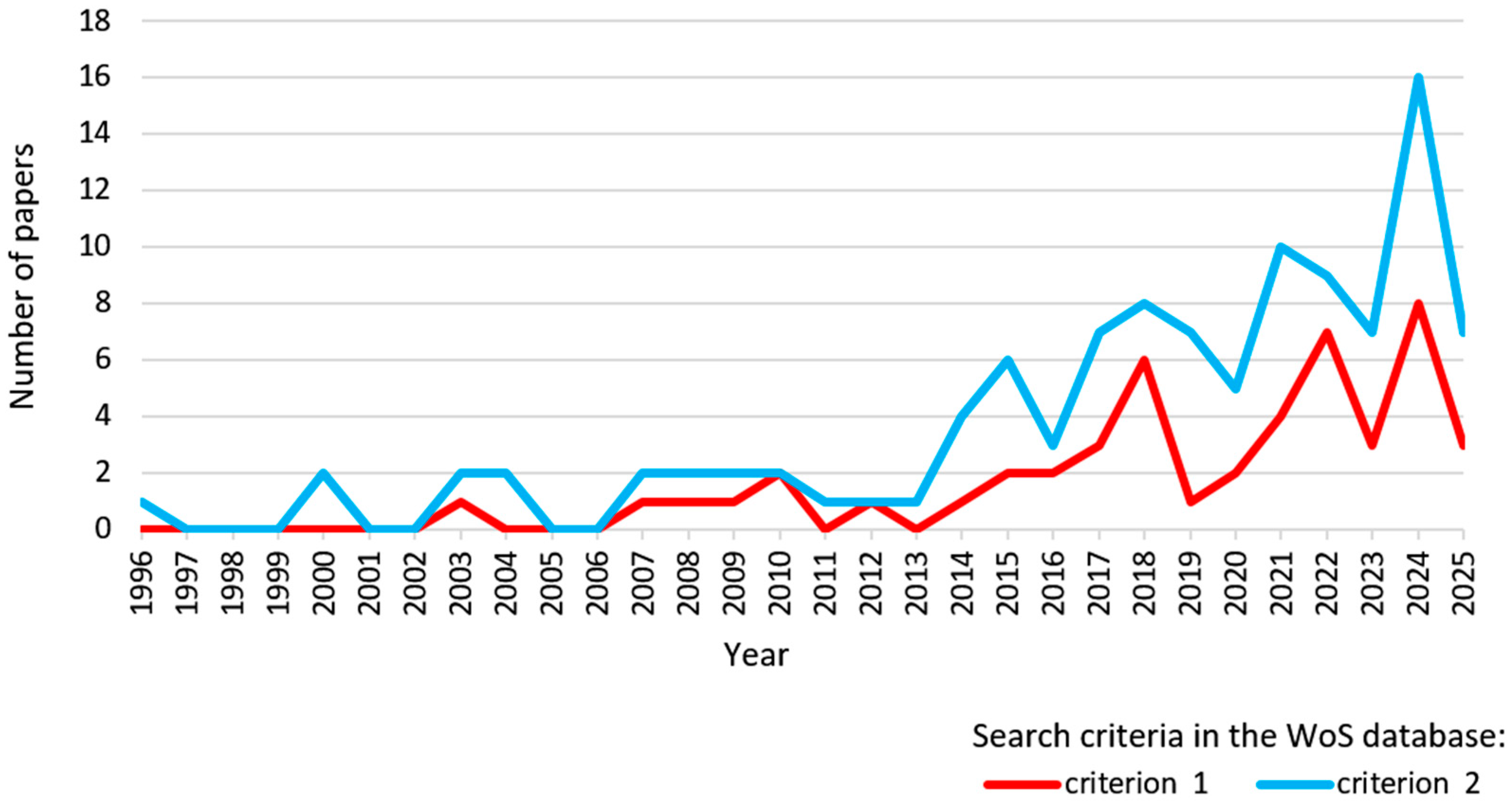
Among the analyzed studies, the earliest paper was published in 2003 for criterion 1 and 1996 for criterion 2, whereas the most recent papers for both criteria were published in 2025. The peak in publication activity occurred in 2024, with 8 and 16 articles for criterion 1 and 2, respectively. The majority of the studies originated from China and the United States, contributing 23 and 16 papers under criterion 1, and 13 and 11 under criterion 2, respectively (Figure 1).

An examination of the thematic distribution of articles identified under criterion 1, encompassing maritime transport, weather conditions, safety, economic aspects, and modeling, based on the WoS subject category classification, highlights the highly interdisciplinary character of this field of research. The largest number of publications (31) was assigned to Engineering. Other prominent fields include Oceanography (23), Environmental Sciences and Ecology (13), and Computer Science (12), highlighting the integration of engineering-oriented safety analysis with environmental processes and advanced computational methods. A similar distribution was observed for criterion 2, with Engineering (31), Oceanography (12), Environmental Sciences and Ecology (6), and Computer Science (6) being the most frequently represented categories. In both cases, relatively few publications were classified under Business Economics (4 and 2, respectively), which confirms that economic aspects are usually treated as secondary outcomes of technical or operational analyses rather than as primary objects of modeling. Single publications were also assigned to research areas such as Operations Research and Management Science, Transportation, Geography, and Mathematics, further illustrating the methodological diversity of the field and the absence of a dominant, unified framework for integrating safety, weather, and cost consideration.

The next stage of the bibliometric study aimed to determine the dominant thematic areas, underexplored topics, and potential future research directions related to operational safety and cost efficiency in maritime transport. For this purpose, a bibliometric methodology was applied based on term co-occurrence analysis and visual representation of the results using the VOSviewer software (version 1.6.20), with bibliographic records retrieved from the WoS database.

VOSviewer is a commonly used tool for bibliometric investigations, allowing the examination of relationships between key concepts and their organization into thematic groupings through network-based visualizations. In such visualizations, individual clusters are distinguished by different colors, enabling the identification of structural patterns and the relative intensity of linkages within the research domain. Keyword co-occurrence maps were generated from the selected publications, where each node represents a specific term and the connecting lines indicate how frequently pairs of terms appear together in the literature. The relative importance of each term is reflected by the size of its node, with larger nodes corresponding to more frequently occurring keywords. In addition to the network analysis, a temporal perspective was introduced through an overlay visualization, in which node colors represent the average year of publication associated with each keyword. This made it possible to trace the evolution of research themes over time and to distinguish established topics from those that are gaining increasing attention, thereby providing insight into both current research priorities and emerging trends.

However, it should be noted that the visualizations presented in this study are based exclusively on publications indexed in the WoS database and therefore do not include potentially relevant contributions available in other sources, such as Scopus or Google Scholar, particularly in the areas of maritime safety and cost studies. The results of the bibliometric analysis should therefore be interpreted in light of this database limitation. However, this does not affect the internal consistency of the analysis, as the study aims to identify trends within a well-defined and widely used bibliographic dataset. Furthermore, the adopted bibliometric approach is inherently quantitative and does not involve a detailed qualitative evaluation of individual studies. Nevertheless, the concept maps generated using VOSviewer offer a meaningful overview of prevailing research directions and shifts in thematic focus within the analyzed field.

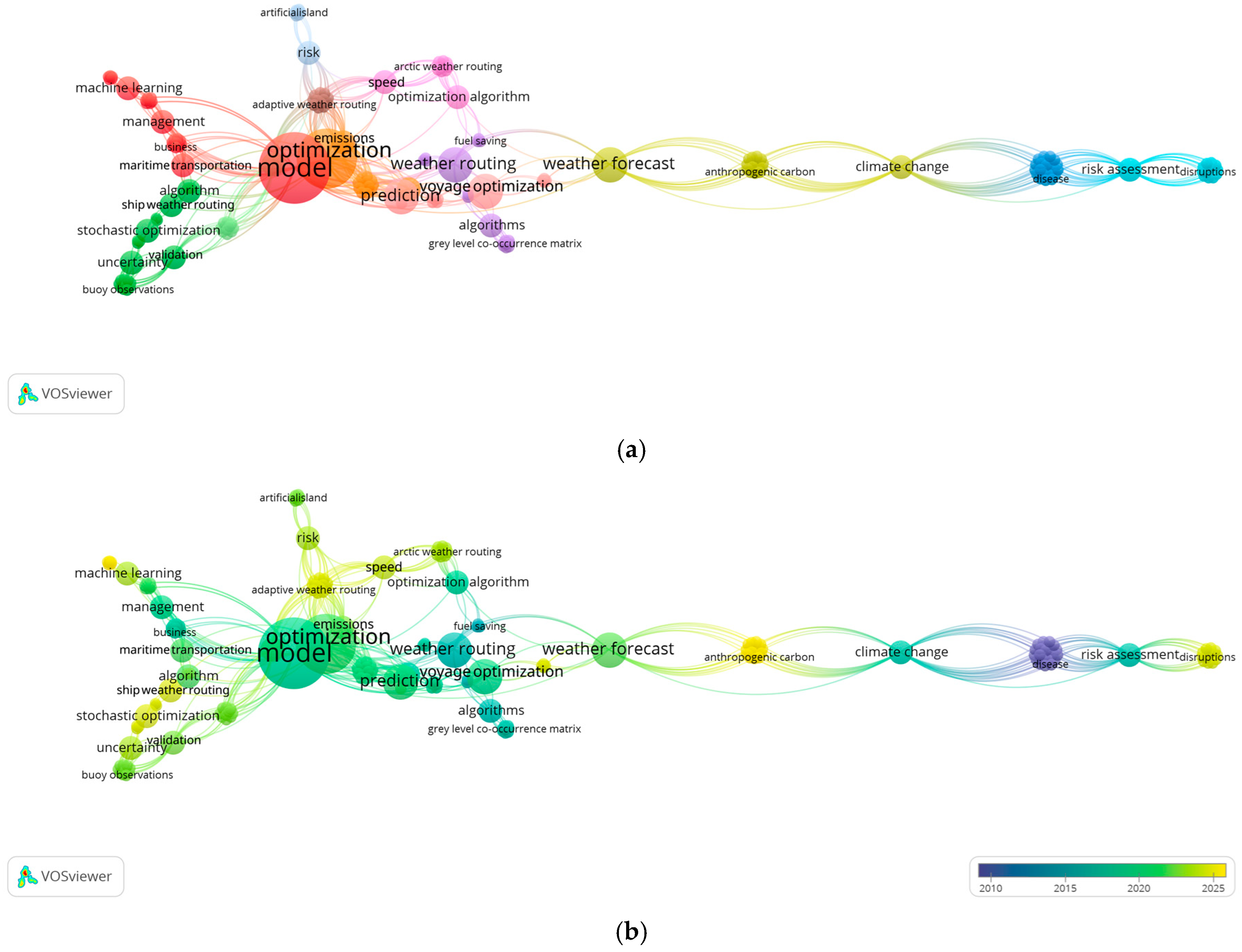
The network visualization (Figure 2a) of keyword co-occurrence for the more restrictive search criterion (criterion 1) reveals a clearly focused yet highly differentiated thematic structure, characteristic of an interdisciplinary research area that integrates modeling, safety, weather, and economic aspects of maritime transport. The central node of the network is the term “model”, which exhibits the highest number of links with other keywords. Its prominent position indicates that the dominant share of the analyzed literature is centered on the formal modeling of decision-making and operational processes, which form the basis for risk assessment, forecasting, and optimization under variable weather conditions. Strong links between the node “model” and terms such as “prediction”, “algorithm”, “optimization algorithm”, and “stochastic optimization” confirm the key role of quantitative and probabilistic methods [21,22,23,24,25,26,27,28,29,30,31,32,33,34,35,36].

On the left side of the visualization, a modeling and optimization cluster (red and green) is visible, centered around terms: “algorithm”, “stochastic optimization”, “uncertainty”, and “machine learning” [29,30,35,37,38,39]. This cluster represents a research stream focused on addressing weather-related uncertainty through advanced computational methods. While it reflects growing interest in these approaches, their relatively peripheral position suggests that they are still mainly used as supporting tools rather than as core components of integrated safety–cost modeling frameworks [40,41,42,43].

A clearly distinguishable cluster related to routing and operational efficiency (purple, brown, orange, and pink) includes the terms “weather routing”, “adaptive weather routing”, “optimization algorithm”, “fuel saving”, and “emissions”. This research stream is primarily concerned with minimizing operational and environmental costs, with safety often treated indirectly as a constraint within route optimization processes [22,23,24,25,26,44,45,46,47,48,49,50,51]. Strong connections between “weather routing” and “prediction” as well as “weather forecast” highlight the importance of meteorological forecasts as key decision-support inputs, however, the absence of direct references to operational safety states suggests a fragmented approach [30,34,52,53,54,55,56,57,58]. The terms “risk” and “risk assessment” form smaller, more isolated clusters related to risk and safety (blue), indicating that while risk evaluation is present in the literature, it is rarely directly integrated with cost analysis or comprehensive decision-support models [59,60]. Safety is more frequently addressed as an element of risk analysis than as a dynamic, weather-dependent operational state [61,62,63,64,65,66]. On the right side of the visualization, an elongated climate-related cluster (olive) includes the terms “weather forecast”, “anthropogenic carbon”, and “climate change”. Its structure suggests weak and indirect linkages between climate-related research and safety or cost modeling. Climate change is therefore mainly analyzed in the context of emissions and long-term environmental trends rather than as a direct factor contributing to the degradation of operational safety [67,68,69,70,71].

The overlay visualization (Figure 2b) illustrates the temporal evolution of research interests in the area of modeling the impact of weather conditions on safety and costs in maritime transport. The earliest studies (dark blue and turquoise nodes) focus on topics such as “weather routing”, “algorithms”, and “prediction”. This indicates that the initial stage of research development was dominated by computational techniques and forecasting approaches, in which weather conditions were primarily treated as inputs to optimization algorithms, without explicit consideration of operational safety or cost consequences. In subsequent years, a shift in research focus towards optimization and operational efficiency can be observed, as reflected by nodes such as “fuel saving”, “emissions”, and “optimization algorithm”. Studies from this period primarily address the reduction of fuel consumption and emissions, often in the context of weather routing, while safety remains an indirect factor, typically treated as a constraint within optimization processes. The most recent studies (yellow nodes) include concepts such as “machine learning”, “stochastic optimization”, “uncertainty”, “risk”, and “adaptive weather routing”. This trend indicates growing interest in probabilistic and adaptive methods that enable dynamic responses to changing weather conditions and explicitly account for uncertainty in decision-making processes. At the same time, the appearance of risk-related terms suggests a gradual shift towards safety-oriented analyses, however, these approaches still lack a clear and systematic linkage to the economic consequences of hazardous events. The “climate change” theme, associated with terms such as “anthropogenic carbon” and “weather forecast”, appears relatively late and remains weakly integrated with mainstream safety modeling. This suggests that the impact of climate change on the operational safety of maritime transport is predominantly examined from an environmental and long-term perspective, rather than as a factor directly influencing day-to-day operational decisions and their associated costs. Notably, the term “model”, despite its central position in the network, exhibits a relatively neutral temporal coloration, indicating that modeling has remained a persistent element of research over time, while its integration with operational safety and cost analysis has evolved gradually and in a fragmented manner.

Considering the VOSviewer visualizations prepared for criterion 1, the results reveal a dispersed network structure and relatively weak linkages between clusters related to probabilistic modeling, safety, and cost analysis. There is a noticeable absence of studies that systematically and quantitatively integrate weather variability, the degradation of operational safety states, and the resulting economic consequences. Current developments in the literature point towards an increasing focus on accounting for weather-related uncertainty, adaptive decision-making models, and probabilistic risk assessment.

The limited number of retrieved records (49) and the lack of regional references, including the Baltic Sea, indicate that existing studies remain fragmented and do not adequately address the specific characteristics of local sea areas or ferry transport operations. In particular, no studies were identified that explicitly examine ferry transport under the distinctive environmental and operational conditions of the Baltic Sea.

These findings substantiate the need to develop a probabilistic model of economic consequences that directly links weather variability with the degradation of operational safety in maritime transport. Addressing this gap constitutes the main contribution of the present study and responds directly to the clearly identified research deficiency.

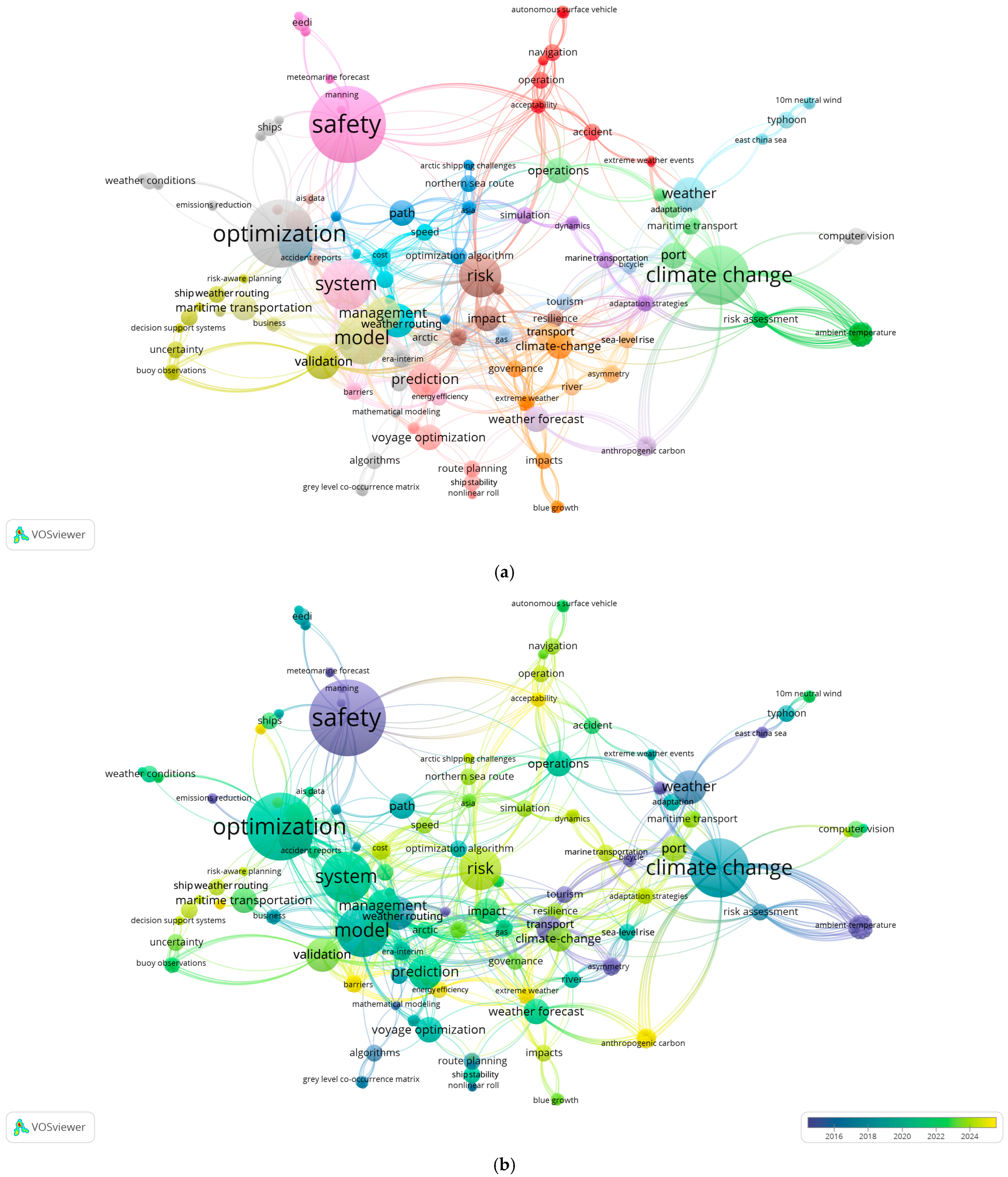
The network visualization (Figure 3a) for the search based on criterion 2 reveals a richer and more complex thematic structure than that observed for criterion 1. However, it should be noted that this criterion does not explicitly include modeling-related keywords. Increasing the number of records to 107 enabled the identification of a larger number of research clusters and stronger interconnections between weather, safety, and cost-related topics in maritime transport.

The network map reveals a strong fragmentation of research across the themes of safety, weather, optimization, and economic impact, alongside the absence of a single dominant research stream that fully integrates these dimensions. Central positions in the network are occupied by the concepts “optimization”, “model”, “system”, and “management”, which act as intermediary nodes linking weather-related, safety-related, and cost-related clusters. Their positioning indicates that system modeling and optimization constitute the primary analytical tools used in the literature; however, they serve more as methodological instruments than as a conceptual framework for integrating safety and economic considerations [21,23,27,34,44,47,72,73,74,75,76]. Strong links between “optimization”, “cost”, “fuel saving”, “speed”, “impact”, and “management” confirm that costs are most often interpreted in terms of operational efficiency, particularly fuel consumption and energy performance rather than as costs arising from safety degradation or undesirable events [77,78,79,80,81,82,83,84,85]. The safety cluster (pink), centered on the concept of “safety”, includes terms such as “manning”, “ships”, “meteomarine forecast”, and concepts related to operational acceptability (“acceptability”—red cluster) [86,87,88]. Its structure suggests that safety is analyzed mainly in organizational and crew-related contexts, in relation to weather hazard forecasting, and in terms of the acceptability of operational risk. However, the links between the safety cluster and economic nodes are weak and indirect, indicating that safety is rarely directly valued in economic terms. A distinct risk (brown) and accident (red) cluster, associated with the concepts “accident”, “risk”, and “operations”, connects both to safety and to weather-related issues [31,38,75,89,90,91,92,93,94]. This indicates that risk and accident analysis serves as a bridge between safety and operations, yet it still does not lead to a clear linkage with the economic costs of hazardous events, such as financial losses, operational downtime, or repair expenses.

A clearly identifiable but peripheral “climate change” cluster (green) encompasses concepts such as “risk assessment”, “ambient temperature”, “anthropogenic carbon”, “sea-level rise”, and “adaptation strategies” [95,96,97]. Its structure indicates that climate change is mainly examined from a macro-scale perspective, with a dominance of environmental and adaptation-related themes, and without direct linkage to the operational costs of individual voyages or to the degradation of day-to-day safety.

The map also reveals specialized thematic threads, such as “Northern Sea route”, “Arctic shipping challenges”, and “autonomous surface vehicle” [39,45,46,98,99,100]. Their presence, particularly in more recent temporal layers, points to growing interest in climatically sensitive regions and the development of new technologies and autonomous systems. Nevertheless, economic quantification of safety-related risks remains largely absent in these contexts. The lack of strong, direct connections between weather, safety, and cost clusters clearly indicates a research gap: the absence of probabilistic models that integrate weather variability, the degradation of operational safety states, and the resulting economic consequences. This gap justifies the need for further research, particularly with regard to ferry transport and region-specific conditions such as those of the Baltic Sea.

The overlay visualization (Figure 3b) for criterion 2 illustrates the temporal evolution of research on the impact of weather conditions on safety and costs in maritime transport, as well as the gradual expansion of the thematic scope of the analyzed field. The color differentiation of the nodes indicates a clear transition from technical and engineering-oriented issues toward more complex, systemic, and interdisciplinary approaches that incorporate managerial, climatic, and economic aspects.

The earliest layer of the literature (nodes in navy blue and purple shades) is represented by concepts such as “safety”, “manning”, “fuel saving”, “weather”, and “ambient temperature”. Research from this period focused primarily on technical aspects of ship safety, vessel stability and behavior under adverse weather conditions, and meteorological forecasting as a source of operational hazards. In this phase, safety was analyzed mainly from an engineering perspective, while links to costs were marginal or indirect, without explicit quantification of the economic consequences of hazards.

The subsequent stage of research development, marked by turquoise and green colors, includes concepts such as “model”, “system”, “management”, “optimization”, “prediction”, “voyage optimization”, “path”, and “speed”. Within this stream, weather begins to be systematically integrated into decision-making processes; mathematical and system-based models dominate route and speed planning; and costs are primarily associated with operational efficiency, fuel consumption, and energy efficiency (“fuel saving”, “impact”). Safety continues to function mainly as a constraint within optimization algorithms rather than as a dynamic operational state directly linked to costs.

An important element of the map is the cluster centered on the concepts “risk”, “accident”, “operations”, and “acceptability”, which connects safety issues with operational processes. This indicates a gradual incorporation of risk analysis into maritime transport research. However, even within this stream, risk is rarely expressed in terms of economic losses, and there remains a lack of coherent models linking the probability of hazardous events with their associated costs.

The most recent studies (yellow nodes) encompass concepts such as “risk assessment”, “adaptation strategies”, “ambient temperature”, “anthropogenic carbon”, “extreme weather”, “resilience”, and regional references (e.g., “Northern Sea route”, “Arctic shipping challenges”). This reflects growing interest in the impact of climate change on maritime transport, the development of adaptive and resilience-based approaches, and risk analysis at macro-operational and environmental scales.

At the same time, the climate change cluster remains relatively peripheral to the optimization and operational safety clusters, suggesting that climate is mainly analyzed from a long-term perspective rather than as a factor directly influencing day-to-day operational decisions and their associated costs. The central position of the concepts “optimization” and “model”, visible across all temporal layers, confirms the dominance of the optimization-oriented approach in the literature. Conversely, the dispersion and peripheral positioning of “safety”, “risk”, and “climate change” indicate that, despite advances in computational and system-based methods, safety, weather, and costs are still largely examined in isolation. There remains a lack of probabilistic models that integrate weather variability, degradation of safety states, and their measurable economic consequences. The results of the overlay visualization analysis confirm the existence of a research gap characterized by the absence of an integrated approach that combines weather, safety, and costs within a single, coherent probabilistic decision-making model, thereby justifying further research in this direction.

Compared to criterion 1, the network analysis for criterion 2 highlights the predominant role of optimization and weather routing in the literature, alongside a clear structural separation between safety-focused analyses and cost-oriented studies, and a marginal, largely indirect treatment of climate change impacts. The lack of strong links between clusters related to weather, safety, and costs confirms that existing studies rarely provide integrated modeling frameworks that probabilistically connect these elements. In particular, no explicit approaches were identified that describe the degradation of operational safety states as a function of weather conditions while simultaneously assigning measurable economic consequences. Consequently, the analysis based on criterion 2 using the WoS database further substantiates the need for the probabilistic cost model proposed in this manuscript, specifically dedicated to ferry transport operations under the environmental and operational conditions of the Baltic Sea.

From a methodological perspective, existing studies addressing maritime weather impacts typically focus on isolated aspects of the problem, including weather-routing optimization, navigational risk assessment, delay propagation, or direct cost estimation under adverse environmental conditions. Many of these approaches rely on simplified flat-state representations of operational conditions, where weather effects are incorporated either through deterministic thresholds or externally imposed cost adjustment factors. While such models provide valuable operational insights, they often do not capture the dynamic and hierarchical nature of operational safety degradation processes in maritime transport systems.

This limitation becomes particularly relevant in the context of sustainable maritime transport, where operational resilience, adaptive decision-making, and efficient risk mitigation increasingly depend on understanding the coupled relationships between environmental uncertainty, safety performance, and operational costs. In contrast to conventional flat-state approaches, the hierarchical semi-Markov framework proposed in this study represents operational safety through multiple interconnected degradation levels with duration-dependent transition dynamics. This enables a more realistic representation of progressive operational deterioration under changing weather conditions, together with its associated economic implications. Consequently, the proposed framework provides an integrated probabilistic approach linking weather variability, safety-state degradation, and operational cost formation in ferry transport systems operating under Baltic Sea conditions.

To clarify the methodological positioning of the proposed framework, a qualitative comparison of representative approaches identified in the literature is presented in

Table 1. Comparative positioning of representative modeling approaches in maritime weather–risk–cost analysis.

Approach Type	Weather Variability	Safety-State Modelling	Cost Implications	Probabilistic Framework	Hierarchical Degradation	Sustainability/Resilience Perspective
Weather-routing optimization	Explicitly addressed	Limited	Indirectly addressed	Partially addressed	Not explicitly considered	Limited
Maritime risk assessment models	Partially addressed	Explicitly addressed	Rarely addressed	Explicitly addressed	Not explicitly considered	Limited
Cost-of-delay approaches	Explicitly addressed	Not explicitly considered	Explicitly addressed	Limited	Not explicitly considered	Rarely addressed
Maritime resilience models	Partially addressed	Partially addressed	Partially addressed	Partially addressed	Not explicitly considered	Explicitly addressed
Proposed framework	Explicitly addressed	Explicitly addressed	Explicitly addressed	Explicitly addressed	Explicitly addressed	Explicitly addressed

.

As summarized in Table 1, existing approaches generally address operational, safety, economic, or resilience-related aspects separately, without fully integrating these dimensions within a unified probabilistic framework. In contrast, the approach proposed in this study combines short-term weather variability, hierarchical safety-state degradation, and operational cost dynamics within a semi-Markov modelling structure. This enables a more realistic assessment of climate-related operational risks and their economic implications in sustainable ferry transport systems operating under Baltic Sea conditions.

While semi-Markov models have been applied to maritime safety [101] and Bayesian networks to maritime risk assessment [62], no existing framework explicitly couples weather variability to safety-state expected lifetime and subsequently to operational costs within a nested safety-subset structure. This integration constitutes the primary novelty of the present study.

3. Materials and Methods

3.1. Theoretical Foundation: The Three-Layer Conceptual Model

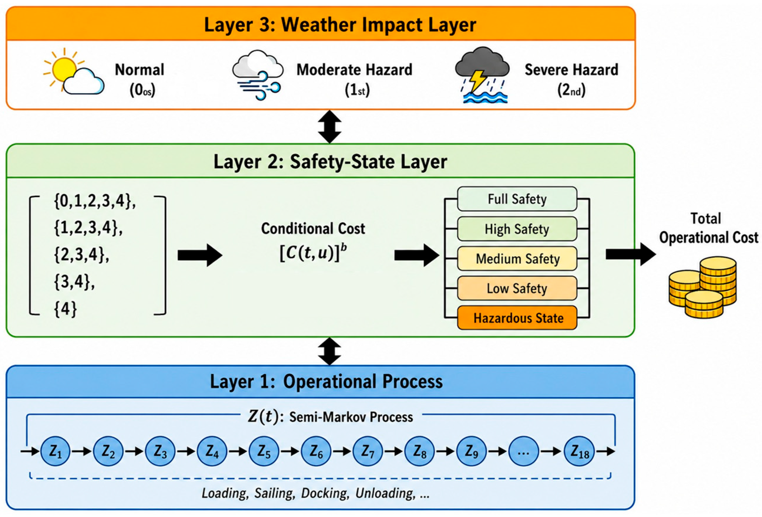
The methodological core of this study is a three-layer probabilistic framework designed to systematically integrate the ferry’s operational cycle, its hierarchical safety state profile, and external weather variability. This integrated structure explicitly models the causal pathway through which meteorological conditions influence operational expenditures by altering the system’s exposure to degraded safety conditions. A schematic representation of this framework is provided in Figure 4.

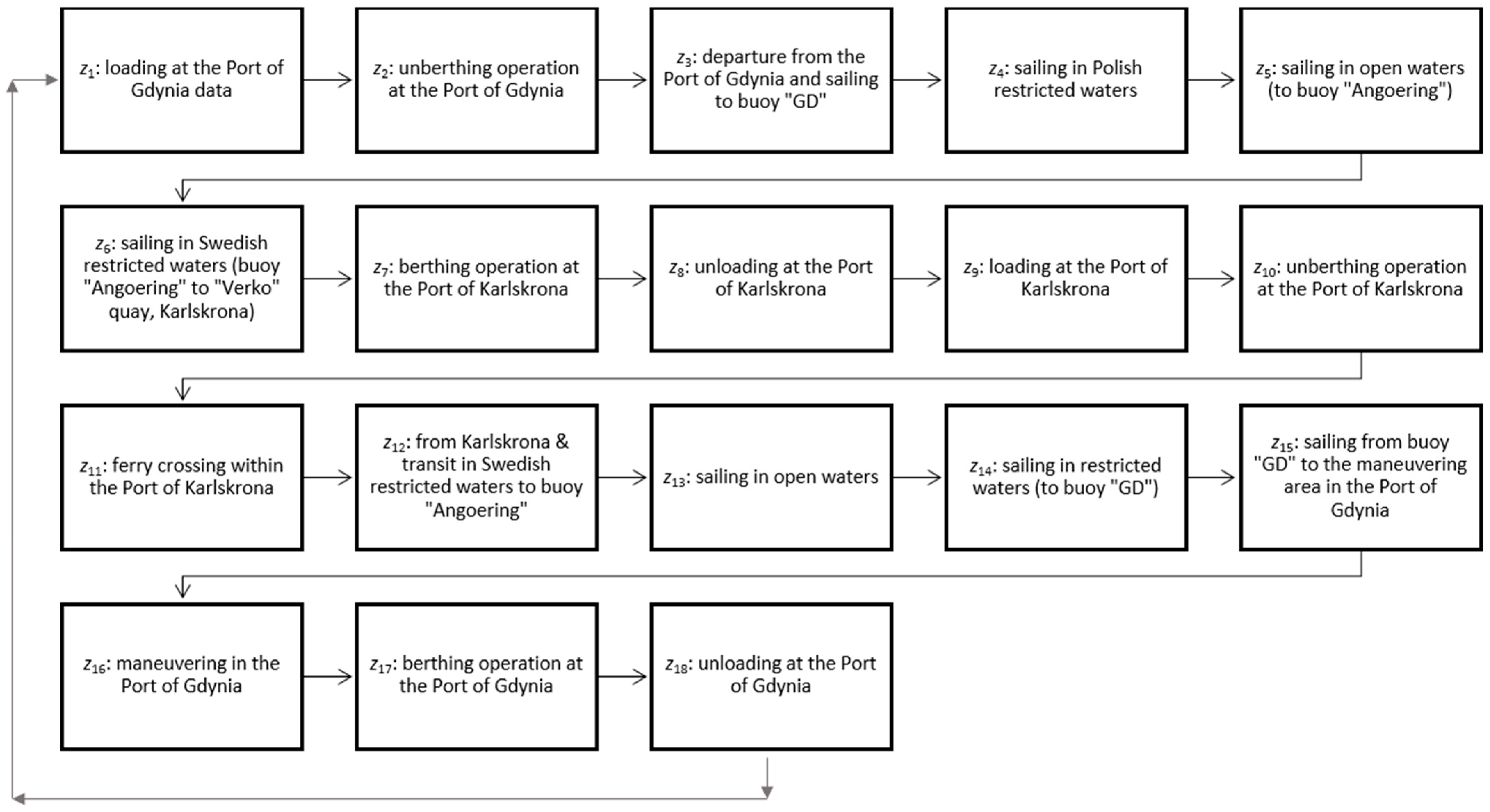
Layer 1: The Operational Process constitutes the foundational layer, representing the sequential cycle of the ferry’s activities. The vessel’s voyage is decomposed into a sequence of 18 discrete operational states, denoted $z_1, z_2,\dots , z_{18}$, corresponding to specific phases such as loading, port maneuvering, open-sea navigation, and unloading. The progression through these states is modeled as a semi-Markov process $Z\left(t\right)$, t ≥ 0. This stochastic formulation captures the quasi-deterministic, schedule-driven nature of the voyage while formally accounting for potential variability in state sojourn times. The semi-Markov approach is chosen for its capacity to model duration-dependent transitions, offering a more realistic representation for systems where the time spent in a state can influence subsequent behavior or degradation [101,102,103,104]. The semi-Markov framework was selected because it enables analytical estimation of expected safety-state lifetimes, which constitute the core mechanism of the proposed cost model. In addition, semi-Markov processes naturally account for duration-dependent state persistence while remaining analytically tractable for the sequential operational structure of ferry transport.

Layer 2: The Safety-State Layer overlays a detailed safety classification onto the operational process. Informed by expert judgment and considerations of operational efficiency and safety, the technical system’s safety condition is categorized into five distinct, ordered states:

• Safety state 4—full safety;
• Safety state 3—high-level safety;
• Safety state 2—medium-level safety;
• Safety state 1—low-level safety;
• Safety state 0—hazardous state.

For the purpose of cost modeling and to analyze system performance under varying conditions, these states are organized into nested safety subsets: {0, 1, 2, 3, 4}, {1, 2, 3, 4}, {2, 3, 4}, {3, 4}, and {4}. The subset {≥u}, where u = 0, 1, 2, 3, 4, includes all safety states from level u to level 4. The crucial link between operation and safety is established via the conditional instantaneous cost [C(t,u)]^(b). This parameter defines the cost rate incurred at time t while the system is in operational state $z_b$, conditional upon the system’s safety level being within the subset {≥u}. These cost rates, assumed constant for a given operational and safety-subset pair, are derived from the aggregated activity, wear, and resource consumption profiles of the vessel’s technical subsystems under the specified safety regime.

Layer 3: The Weather Impact Layer introduces environmental variability as the external driver of system dynamics. Weather conditions along the ferry route are represented as a stochastic process W(t), classified into three discrete hazard categories: normal conditions (0os), moderate hazard (1st-degree), and severe hazard (2nd-degree). The novel mechanism of weather influence proposed in this model operates through the safety layer. The weather process W(t) does not directly scale costs but is theorized to modify the system’s safety state dynamics. Adverse weather conditions increase the probability of transitions to lower safety states and, critically, prolong the expected lifetime within these degraded states. Therefore, the primary output of this layer’s influence is a weather-modified expected conditional lifetime, denoted [µ_β($\ge$u)]^(b). This parameter represents the expected duration the system spends in safety subset {$\ge$u}, given it is in operational state $z_b$, under the influence of a specific weather regime w. It should be noted that the expected lifetimes obtained from the model are expressed in calendar time units (years) and should be interpreted as reliability-based indicators of the persistence of a given safety state, rather than as direct representations of operational voyage durations.

The interdependence of these layers creates a coherent causal chain: external weather perturbations (Layer 3) alter the intrinsic safety state occupancy profile (Layer 2) of a system following its scheduled operational cycle (Layer 1). This alteration manifests as increased exposure to lower, more costly safety states. When these modified expected lifetimes are combined with the state- and safety-subset-dependent cost rates, the total weather-influenced operational cost can be obtained. This three-layer structure provides a transparent and physically interpretable foundation for quantifying how meteorological uncertainty translates into financial risk for maritime transport systems by fundamentally altering their operational safety profile.

3.2. Mathematical Model of the Operational Process

The functioning of a complex technical system, such as a ferry vessel, is represented by a semi-Markov process $Z\left(t\right)$, $t\ge 0,$ [101,102,103,105]. The process evolves over a finite set of discrete operational states, $A=\left\{z_1,\hspace{0.33em}{z}_2,\dots ,z_{\nu }\right\},$ where for the ferry system under consideration ν = 18. Each state $z_b$ corresponds to a specific phase of the operational cycle, including, for example, loading operations, navigation in open waters, or port maneuvering. The semi-Markov process $Z\left(t\right)$ is fully characterized by the following elements.

• Initial state distribution

The initial probabilities are collected in the vector

$${\left[p_b\left(0\right)\right]}_{1x\nu }=\left[p_1\left(0\right),p_2\left(0\right),\dots ,p_{\nu }\left(0\right)\right],$$

(1)

where $p_b\left(0\right)=P\left(Z\left(0\right)=z_b\right)$, b = 1, 2, …, ν.

• Transition probability matrix

State-to-state transitions are governed by the following matrix:

$${\left[p_{bl}\right]}_{v\mathrm{x}v}=\left[\begin{array}{cc}\begin{array}{cc}{p}_{11}& p_{12}\\ p_{21}& p_{22}\end{array}& \begin{array}{cc}\dots & p_{1v}\\ \dots & p_{2v}\end{array}\\ \begin{array}{cc}⋮& ⋮\\ p_{v1}& p_{v2}\end{array}& \begin{array}{cc}\ddots & ⋮\\ \dots & p_{vv}\end{array}\end{array}\right],$$

(2)

where $p_{bl}$ denotes the probability that the process enters state $z_l$ immediately after leaving state $z_b,$ for (b ≠ l). Self-transitions are excluded, hence $p_{bb}=0$ for all b.

• Conditional sojourn time distributions

The duration of time spent in a given state before transitioning to another state is described by the matrix of conditional distribution functions:

$${\left[H_{bl}\left(t\right)\right]}_{v\mathrm{x}v}=\left[\begin{array}{cc}\begin{array}{cc}{H}_{11}\left(t\right)& H_{12}\left(t\right)\\ H_{21}\left(t\right)& H_{22}\left(t\right)\end{array}& \begin{array}{cc}\dots & H_{1v}\left(t\right)\\ \dots & H_{2v}\left(t\right)\end{array}\\ \begin{array}{cc}⋮& ⋮\\ H_{v1}\left(t\right)& H_{v2}\left(t\right)\end{array}& \begin{array}{cc}\ddots & ⋮\\ \dots & H_{vv}\left(t\right)\end{array}\end{array}\right]$$

(3)

where

$$H_{bl}\left(t\right)=P\left({\theta }_{bl}<t\right), t\ge 0, b, l=1, 2, \dots , v, b\ne l.$$

Here, ${\theta }_{bl}$ is the random variable representing the sojourn time in state $z_b$, conditional on the next transition being to state $z_l$.

The corresponding mean conditional sojourn times are defined as

$$M_{bl}=E\left[{\theta }_{bl}\right]{\displaystyle {\int }_0^{\infty }}td{H}_{bl}\left(t\right)={\displaystyle {\int }_0^{\infty }}t{h}_{bl}\left(t\right)dt,$$

(4)

where $h_{bl}\left(t\right)$ denotes the probability density function associated with $H_{bl}\left(t\right)$.

• Limiting state probabilities

For a semi-Markov process operating in steady state, the long-run probability of finding the system in state $z_b$ is given by

$$p_b=\underset{t\to \infty }{\mathrm{l}\mathrm{i}\mathrm{m}}{p}_b\left(t\right)={\displaystyle \frac{{\pi }_b{M}_b}{{\displaystyle {\sum }_{l=1}^v}{\pi }_l{M}_l}}, b=1, 2, \dots , v.$$

(5)

In this expression,

$$M_b={\displaystyle \sum _{l=1}^v}{p}_{bl}{M}_{bl}$$

is the unconditional mean sojourn time in state $z_b$, while π_b denotes the stationary probabilities of the embedded Markov chain. The vector [π_b] satisfies

$$\left\{\begin{array}{c}\left[{\pi }_b\right]=\left[{\pi }_b\right]\left[p_{bl}\right]\\ {\displaystyle {\sum }_{l=1}^v}{\pi }_l=1.\end{array}\right.$$

(6)

Model specialization for the case study: In the analyzed case, the ferry operates according to a fixed and repeating operational schedule imposed by the operator. As a result, the transition structure between states is deterministic, and the transition probabilities $p_{bl}$ take binary values (0 or 1). Under these conditions, the semi-Markov process reduces to a cyclic semi-Markov model.

This formulation preserves the advantages of the semi-Markov framework, most notably, the ability to model random sojourn times and correlated external disturbances such as weather effects while allowing direct use of limiting-state formulas to evaluate time allocation and cost accumulation based on planned operational sequences.

The adopted semi-Markov representation intentionally simplifies certain operational aspects of ferry transport. In particular, the current framework assumes a predefined operational sequence and does not explicitly model unscheduled disruptions, cumulative fatigue effects, or gradual operational transitions. These simplifications are acceptable for the present methodological demonstration, which focuses on isolating the causal relationship between weather variability, safety degradation, and operational cost accumulation.

Consequently, over a fixed operational horizon [0, θ], the expected total time spent in state $z_b$ can be approximated as

$${\widehat{M}}_b=E\left[{\widehat{\theta }}_b\right]=p_b\theta , b=1, 2, \dots , v.$$

(7)

Equation (7) represents an asymptotic result, which becomes increasingly accurate as the operational horizon grows and the semi-Markov process converges to its stationary regime. This expression provides the probabilistic basis for allocating time across operational states and serves as a foundation for the cost analysis developed in the subsequent sections.

3.3. Safety Subset Cost Model

3.3.1. Conditional Instantaneous Costs

The fundamental assumption of the cost model is that the operational cost structure of the ferry is intrinsically linked to its safety configuration. It is assumed that individual operational states $z_b$∈ A, where b = 1, 2, …, ν, and ν = 18, influence the system’s functional structure, its safety configuration, and consequently, its instantaneous operational expenditure [104,105,106].

For each operational state $z_b$, we define the vector of conditional instantaneous costs across the nested safety subsets:

$${\left[\mathit{C}\right(t,·\left)\right]}^{\left(b\right)} ={\left[\right[\mathit{C}(t, \ge 1)]}^{\left(b\right)}, {\left[\mathit{C}\right(t, \ge 2\left)\right]}^{\left(b\right)}, \dots , {\left[\mathit{C}\right(t, 4]}^{\left(b\right)}], t\ge 0,$$

(8)

where the component [C(t,$\ge u$)]^(b), for $u=1, 2, 3, 4,$ represents the conditional instantaneous cost rate. This is the cost per unit time incurred when the semi-Markov process $Z\left(t\right)$ is in the operational state $z_b$ and the system’s safety level belongs to the subset {$u$, $u$ + 1, …, 4}. In other words, it is the cost rate applicable given that the system’s safety is at least at level $u$. A core simplification adopted for this case study is that these conditional cost rates are constant over time for a given pair of operational state and safety subset. Therefore, we denote them simply as $C_{b,u}$:

$${\left[\mathit{C}\right(t, \ge u\left)\right]}^{\left(b\right)} = C_{b,u}, \mathrm{for} \mathrm{all} t\ge 0.$$

(9)

The values of $C_{b,u}$ were established via a structured expert elicitation process involving senior ferry operators and marine engineers with extensive experience on the Gdynia–Karlskrona route. It is important to emphasize that these cost rates are not estimated statistically from operational accounting data but rather elicited from experts to represent internally consistent relative cost intensities across different operational states and safety regimes. This process ensured that the costs reflect realistic subsystem utilization profiles, accounting for factors such as energy consumption, component wear, required crew attention, and maintenance intensity specific to each operational phase and implied safety condition.

The complete set of these parameters forms a cost matrix, which is the essential input for the safety subset cost model. For illustration, the cost rate for operational state $z_1$ (loading at Gdynia) is constant across all safety subsets, as the loading activity incurs the same subsystem costs regardless of the vessel’s overall safety level during this port operation:

$${\left[\mathit{C}\right(t, \ge 1\left)\right]}^{\left(1\right)} = {\left[\mathit{C}\right(t, \ge 2\left)\right]}^{\left(1\right)} = {\left[\mathit{C}\right(t, \ge 3\left)\right]}^{\left(1\right)} = {\left[\mathit{C}\right(t, \ge 4\left)\right]}^{\left(1\right)} = 93c,$$

(10)

where c is a scaling coefficient (e.g., c = 1 PLN for model demonstration). The full matrix of conditional instantaneous costs $C_{b,u}$ for all 18 operational states and the four defined safety subsets ($u=1, 2, 3, 4$) is presented in

Table 2. The conditional instantaneous costs $C_{b,u}$ (in units of c) for operational states $z_b$ and safety subsets {$\ge u$}.

b	State zb	Cb,1 ({≥1})	Cb,2 ({≥2})	Cb,3 ({≥3})	Cb,4 ({≥4})
1	Loading at Gdynia	93	93	93	93
2	Unberthing at Gdynia	145	145	145	145
3	Departure from Gdynia	120	120	120	120
4	Sailing (Polish waters)	103	103	103	103
5	Sailing (open waters)	103	103	103	103
6	Sailing (Swedish waters)	123	123	123	123
7	Berthing at Karlskrona	145	145	145	145
8	Unloading at Karlskrona	83	83	83	83
9	Loading at Karlskrona	83	83	83	83
10	Unberthing at Karlskrona	145	145	145	145
11	Crossing Karlskrona port	120	120	120	120
12	Departure from Karlskrona	103	103	103	103
13	Sailing (open waters, return)	103	103	103	103
14	Sailing (restricted, return)	103	103	103	103
15	Sailing to Gdynia area	120	120	120	120
16	Maneuvering in Gdynia	120	120	120	120
17	Berthing at Gdynia	145	145	145	145
18	Unloading at Gdynia	93	93	93	93

Note: The coefficient c is a scaling factor that can be calibrated against actual accounting data. The model focuses on costs attributable directly to the operation of the technical subsystems.

.

It should be noted that in the present case study the conditional instantaneous cost rates $C_{b,u}$ do not vary across safety subsets for a given operational state. This reflects the assumption that weather-induced safety degradation primarily affects the duration of exposure to different safety regimes, rather than directly modifying instantaneous subsystem cost rates. Consequently, the weather-related cost effect emerges through changes in safety subset expected lifetime rather than through changes in instantaneous cost intensity. This simplification was introduced intentionally to isolate the causal mechanism of interest and improve the interpretability of the framework.

Cost interpretation for nested safety subsets. The cost $\widehat{\mathit{C}}\left(\ge u\right)$ represents the total expected operational expenditure incurred while the system is required to maintain a safety level of at least u. This conceptualization is crucial: if the system’s instantaneous safety state falls below level u (i.e., into states k < u), additional compensatory operational measures are triggered such as reduced speed, increased crew attention, or activation of backup systems to mitigate the elevated risk and effectively maintain the required safety threshold. These mitigation efforts incur the incremental costs ΔC(k) associated with the lower states. Consequently, the cost of operating within subset {≥u} accumulates contributions from all safety states k = 1, …, 4, weighted by the time spent in each state and the compensation required when k < u.

It should be noted that in the present case study the conditional instantaneous cost rates $C_{b,u}$ do not vary across safety subsets for a given operational state. This modeling choice reflects the assumption that weather and safety degradation primarily affect the duration of exposure to safety regimes, rather than directly altering instantaneous subsystem cost rates. As a result, the entire weather-induced cost effect in the proposed framework emerges through modifications of safety subset expected lifetime, ensuring a clear separation between cost intensity and safety state dynamics.

We define the incremental cost rate ${\left[\Delta C\left(k\right)\right]}^{\left(b\right)}$ associated with operating at exact safety state k, (k = 1, 2, 3, 4) during operational state $z_b.$ This represents the additional instantaneous cost incurred when the system’s safety level is exactly k, compared to being at level k − 1. These rates are derived from the conditional subset costs $C_{b,u}$ in Table 2 via the relation: ${\left[\Delta C\left(k\right)\right]}^{\left(b\right)}=C_{b,k}-C_{b,k+1},$ with $C_{b,5}=0.$ Consequently, the conditional cost for subset {≥u} can be expressed as the sum of incremental costs: $C_{b,u}={\displaystyle {\sum }_{k=u}^4}{\left[\Delta C\left(k\right)\right]}^{\left(b\right)}.$

3.3.2. Expected Safety-Subset Lifetimes (Without Weather Influence)

The second fundamental component of the safety-subset cost model is the duration for which the system operates within a given safety regime. For each operational state $z_b$, we define the expected conditional lifetime, denoted as [µ($\ge$u)]^(b). The parameter [µ($\ge$u)]^(b) represents the expected time until the technical system exits the safety subset {$u$,$u$ + 1, …, 4}, conditional on the system being in operational state $z_b$. Thus, it is a reliability-based lifetime measure associated with maintaining, at least, safety level ($\ge$u) rather than a calendar-time share within a fixed operational horizon.

Formally, it is the expected value of the conditional time [T(u)]^(b), representing the time until the system exits the specified safety subset while in operational state $z_b$:

$${\left[\mathit{\mu }\right(\ge u\left)\right]}^{\left(b\right)} =E\left[{\left[T\left(u\right)\right]}^{\left(b\right)}\right], u = 1, 2, 3, 4, b = 1, 2, \dots , 18.$$

(11)

Equivalently, this expected lifetime can be interpreted through the corresponding survival function. It reflects the accumulation over time of the probability that the system remains within the safety subset {$u$,$u$ + 1, …, 4}, i.e., has not yet exited this subset by time t.

These expected lifetimes are derived from a semi-Markov model of the ferry’s technical system’s safety state transitions, independent of the operational process $Z\left(t\right).$ The model analyzes the stochastic evolution of the system through its five safety states. The output of this analysis is the set of expected conditional times [µ($\ge$u)]^(b), which describe how long, on average, the system maintains a safety level of at least u during each distinct operational phase $z_b.$ For the purposes of this integrated cost model, these values are treated as known input parameters, calculated a priori from the safety and reliability analysis of the vessel’s subsystems [71,101,107].

For clarity, it should be emphasized that the reported lifetime values do not correspond to individual voyage durations. Instead, they represent expected persistence times of safety states derived from the underlying reliability structure of the system. These values should therefore be interpreted in a relative sense, allowing comparison between different operational conditions rather than as direct time measures.

The values are expressed in consistent time units (years in this case). For example, during operational state $z_1$(loading at Gdynia), the expected lifetime associated with maintaining the safety subset {1} equals approximately 1.70476 years in the broadest safety subset {$\ge$1} (which includes all non-hazardous states), and 1.41708 years in the more restrictive subset {$\ge$2} (high-level safety and above), and so on:

$${\left[\mathit{\mu }\right(\ge 1\left)\right]}^{\left(1\right)} \cong 1.70476, {\left[\mathit{\mu }\right(\ge 2\left)\right]}^{\left(1\right)} \cong 1.41708, {\left[\mathit{\mu }\right(\ge 3\left)\right]}^{\left(1\right)} \cong 1.22861, {\left[\mathit{\mu }\right(4\left)\right]}^{\left(1\right)} \cong 1.11601.$$

(12)

The complete matrix of expected conditional expected lifetime [µ($\ge$u)]^(b) for all operational states b = 1, 2, …, 18, and safety subsets u = 1, …, 4 is presented in

Table 3. Expected safety-subset lifetimes [µ($\ge$u)]^(b) [years] for operational states $z_b$ and safety subsets {$\ge$u}.

b	State ${\mathit{z}}_{\mathit{b}}$	[µ(≥1)](b)	[µ(≥2)](b)	[µ(≥3)](b)	[µ(≥4)](b)
1	Loading at Gdynia	1.70476	1.41708	1.22861	1.11601
2	Unberthing at Gdynia	1.60772	1.32879	1.18936	1.06574
3	Departure from Gdynia	1.68087	1.39120	1.24553	1.11512
4	Sailing (Polish waters)	1.69560	1.39303	1.24632	1.11522
5	Sailing (open waters)	1.69547	1.39292	1.24619	1.11510
6	Sailing (Swedish waters)	1.67434	1.37699	1.23228	1.10301
7	Berthing at Karlskrona	1.54736	1.27865	1.15851	1.02847
8	Unloading at Karlskrona	1.72871	1.43719	1.26722	1.13163
9	Loading at Karlskrona	1.72871	1.43719	1.26722	1.13163
10	Unberthing at Karlskrona	1.60772	1.32879	1.18936	1.06574
11	Crossing Karlskrona port	1.61020	1.33360	1.19593	1.07262
12	Departure from Karlskrona	1.70148	1.39692	1.24985	1.11836
13	Sailing (open waters, return)	1.69547	1.39292	1.24619	1.11510
14	Sailing (restricted, return)	1.68630	1.38540	1.23945	1.10910
15	Sailing to Gdynia area	1.68087	1.39120	1.24553	1.11512
16	Maneuvering in Gdynia	1.61025	1.33360	1.19593	1.07262
17	Berthing at Gdynia	1.54736	1.27865	1.15851	1.02847
18	Unloading at Gdynia	1.70476	1.41708	1.22861	1.11601

. This matrix provides the temporal dimension necessary for transforming the instantaneous cost rates from Table 2 into total expected costs.

The values [µ($\ge$u)]^(b) originate from previously published semi-Markov reliability and safety analyses of the ferry’s technical system developed in earlier works [101,106,107]. These studies provide the mathematical derivation of the transition structure and the analytical procedure used to determine the expected times until the system exits a given safety subset {≥u} under individual operational states. In the present study, these values are used as input parameters for the proposed weather–safety–cost framework rather than being re-derived.

All values are expressed in years and represent expected safety-subset lifetimes derived from the reliability model. They are not restricted to a fixed one-year operational horizon.

These expected lifetimes are critical for the model, as they encode the system’s reliability and safety characteristics during different operational phases. They are independent of external weather conditions at this stage, representing the baseline, intrinsic safety-time profile of the ferry’s technical system. The subsequent integration of weather variability will operate by modifying these baseline expected lifetimes.

3.3.3. Baseline Cost Calculation per Safety Subset

Integrating the components defined in the previous subsections, we now calculate the baseline expected operational costs for the ferry system, categorized by its safety state subsets under normal (weather-independent) conditions. This aggregation follows the theoretical framework established for multi-state safety systems [101,104,105].

The total expected operational cost incurred while the system is in safety subset {$\ge$u}, given that it is in a specific operational state $z_b$, is obtained by combining the conditional instantaneous cost rate with the expected duration of exposure to that safety regime. This is formalized by the equation

$${[\widehat{\mathit{C}}(\ge u)]}^{\left(b\right)}={\left[\mathit{\mu }\right(\ge u\left)\right]}^{\left(b\right)} · C_{b,u}, u = 1, 2, 3, 4, b = 1, 2, \dots , 18.$$

(13)

Here, $C_{b,u}$ is the constant conditional cost rate from Table 2 (equivalent to [C($t,$u)]^(b)), and [µ($\ge$u)]^(b) is the expected conditional lifetime from Table 3. The product [$\widehat{\mathit{C}}$($\ge$u)]^(b) therefore represents the total cost contribution from operational state $z_b$ attributable to operation within safety subset {≥u}. To obtain the total expected cost for the entire system within a given safety subset {≥u}, we take the expectation over all operational states. This is calculated as the weighted sum of the state specific costs, where the weights are the limiting probabilities $p_b$ of the semi-Markov operational process Z(t), as derived in Section 3.2. The formula is:

$$\widehat{\mathit{C}}\left(\ge u\right)={\displaystyle {\sum }_{b=1}^{18}}{p}_b[\widehat{\mathit{C}}(\ge u)](b), u = 1, 2, 3, 4.$$

(14)

Interpretation of safety-subset costs: It is important to emphasize that the costs associated with the nested safety subsets {$\ge$u} are not mutually exclusive and are not additive across u. Each subset {$\ge$u} represents the cumulative expected operational cost incurred while the system remains at or above safety level u, rather than the cost of operating exclusively in a single safety state. Consequently, only the cost associated with the broadest subset {$\ge$1} can be interpreted as the total expected operational cost of the system, while costs for higher subsets ({$\ge$2}, {$\ge$3}, {4}) serve as analytical indicators of the economic effort required to maintain increasingly stringent safety thresholds.

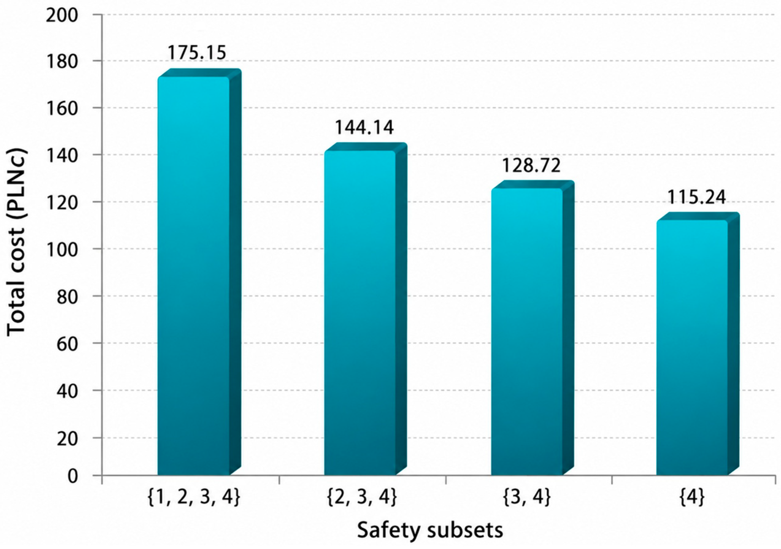
Applying Equations (13) and (14) using the parameters from Table 2 and Table 3 and the limiting probabilities $p_b$ [101,104,106], we obtain the baseline (normal weather) expected costs for each nested safety subset. The results are as follows:

$$\begin{gathered} \widehat{\mathit{C}}(\ge 1) \cong 175.15054\mathrm{c} \mathrm{PLN}, \widehat{\mathit{C}}(\ge 2) \cong 144.13643\mathrm{c} \mathrm{PLN}, \\ \widehat{\mathit{C}}(\ge 3) \cong 128.71551\mathrm{c} \mathrm{PLN}, \widehat{\mathit{C}}(\ge 4) \cong 115.24016\mathrm{c} \mathrm{PLN}. \end{gathered}$$

(15)

They represent the fundamental financial output of the model under reference conditions, prior to the introduction of weather variability. The cost naturally decreases for higher, more restrictive safety subsets (e.g., {4}) as these subsets represent operation in the most reliable and least costly safety states only. The subset {≥1}, which includes all non-hazardous states, carries the highest cost as it encompasses the full spectrum of potential operational expenditures.

This baseline calculation establishes the reference economic performance of the ferry’s technical system. The subsequent section introduces the mechanism through which short-term weather variability perturbs this baseline by modifying the core parameters [µ($\ge$u)]^(b), thereby altering the expected costs $\widehat{\mathit{C}}\left(\ge u\right)$.

3.4. Integration of Short-Term Weather Variability

The cost model developed in the preceding section represents the system’s economic performance under baseline operating conditions, assuming the absence of external environmental disturbances. In the context of ferry operations in the Baltic Sea, such an assumption is insufficient, as short-term meteorological variability constitutes a key driver of operational safety and cost dynamics. To ensure a realistic representation of operational conditions, weather effects are incorporated into the model through their influence on the stochastic structure of the operational process rather than through direct cost adjustments.

In particular, meteorological conditions are assumed to affect operational costs indirectly by modifying the expected conditional expected lifetime of safety-related operational states. Since these expected lifetimes determine the proportion of time spent in different operational regimes, weather-induced changes in safety dynamics act as the primary transmission mechanism between environmental variability and economic performance.

3.4.1. Weather Process and Hazard Classification

Hydro-meteorological conditions represent a dominant external factor influencing maritime transport operations, especially in semi-enclosed basins such as the Baltic Sea. Variations in wind intensity, wave height, and seasonal ice conditions affect propulsion loads, maneuvering effort, and subsystem utilization, thereby altering operational durations and increasing maintenance and operating costs. Moreover, Baltic weather is characterized by pronounced temporal clustering, where sequences of adverse conditions may persist and generate cumulative operational impacts [71,105,108,109,110,111]. To capture these characteristics, weather conditions are modeled as a stochastic process with a finite number of discrete hazard states, represented within a semi-Markov framework. Each hazard state is defined by a set of environmental thresholds and is associated with characteristic transition probabilities and lifetime distributions. This formulation enables the probabilistic integration of meteorological uncertainty into the operational safety and cost model.

The procedures for meteorological data processing, weather state classification, and estimation of transition and residence characteristics follow the methodological framework established in earlier studies (see [71,105,108,109,110,111]). Building on this approach, three levels of weather-related hazard are distinguished, corresponding to increasing degrees of operational impact:

• 0os hazard (no hazard)—conditions corresponding to normal weather, with negligible influence on operations and costs;
• 1st-degree hazard (moderate hazard)—conditions leading to increased operational stress, moderate disruptions, and elevated costs;
• 2nd-degree hazard (severe hazard)—extreme conditions associated with high operational risk, potential downtime, and substantial cost escalation.

Based on expert consultations with ferry operators and maritime engineers, the meteorological parameters most relevant for operational performance along the Gdynia–Karlskrona ferry route were identified. As a result, four spatially distinct weather processes were defined, corresponding to the main segments of the operational cycle:

• weather conditions in the Gdynia Port area;
• weather conditions in Puck Bay (coastal waters);
• weather conditions in Baltic Sea open waters;
• weather conditions in the Karlskrona Port area.

Meteorological input data, including wind speed, wind direction, and significant wave height, were obtained from the ERA5 reanalysis dataset and validated against in situ observations from coastal stations operated by the Institute of Meteorology and Water Management in Poland and the Swedish Meteorological and Hydrological Institute. The analysis covers a six-year period with a temporal resolution of three hours, resulting in 105,602 observations from seven stations located along the transport corridor. Detailed information on the dataset, station locations, and seasonally differentiated probabilities is provided in [105].

For port areas (Gdynia and Karlskrona), wind speed and wind direction were identified as the primary weather-related factors influencing operational costs, whereas for Puck Bay and Baltic Sea open waters, both wind speed and significant wave height were found to be critical. Based on expert-defined threshold values, discrete weather states were classified for each operational area. The resulting classifications are presented in

Table 4. Weather hazard categories and threshold conditions for port operations in Gdynia.

Weather State	Wind Speed	Wind Direction	Hazard Category †
$c_1$	$[0, 17)$ m/s	$\left[0°,22.5°\right)\cup \left[67.5°, 112.5°\right)\cup [337.5°,360°)$	1st
$c_2$	$[17, 33)$ m/s	$\left[0°,22.5°\right)\cup \left[67.5°, 112.5°\right)\cup [337.5°,360°)$	2nd
$c_3$	$[0, 17)$ m/s	$\left[22.5°,67.5°\right)\cup [112.5°,247.5°)$	0
$c_4$	$[17, 33)$ m/s	$\left[22.5°,67.5°\right)\cup [112.5°,247.5°)$	1st
$c_5$	$[0, 17)$ m/s	$[247.5°,337.5°)$	1st
$c_6$	$[17, 33)$ m/s	$[247.5°,337.5°)$	2nd

† Hazard categories: 0os—no hazard (normal operations); 1st—moderate hazard (increased stress); 2nd—severe hazard (extreme conditions, high risk). Threshold values follow the classification framework introduced in [105].

,

Table 5. Weather hazard categories and threshold conditions for port operations in Karlskrona.

Weather State	Wind Speed	Wind Direction	Hazard Category †
$c_1$	$[0, 17)$ m/s	$\left[0°,67.5°\right)\cup [292.5°,360°)$	0os
$c_2$	$[17, 33)$ m/s	$\left[0°,67.5°\right)\cup [292.5°,360°)$	1st
$c_3$	$[0, 17)$ m/s	$[67.5°,157.5°)$	1st
$c_4$	$[17, 33)$ m/s	$[67.5°,157.5°)$	2nd
$c_5$	$[0, 17)$ m/s	$[157.5°,292.5°)$	0os
$c_6$	$[17, 33)$ m/s	$[157.5°,292.5°)$	1st

† Hazard categories: 0os—no hazard (normal operations); 1st—moderate hazard (increased stress); 2nd—severe hazard (extreme conditions, high risk). Threshold values follow the classification framework introduced in [105].

and

Table 6. Weather hazard state definitions for coastal and open-sea navigation segments.

Weather State	Wave Height	Wind Speed	Hazard Category †
$c_1$	$[0, 2)$ m	$[0, 17)$ m/s	0os
$c_2$	$[2, 5) \mathrm{m}$	$[0, 17)$ m/s	0os
$c_3$	$[5, 14) \mathrm{m}$	$[0, 17)$ m/s	1st
$c_4$	$[0, 2) \mathrm{m}$	$[17, 33)$ m/s	1st
$c_5$	$[2, 5) \mathrm{m}$	$[17, 33)$ m/s	1st
$c_6$	$[5, 14) \mathrm{m}$	$[17, 33)$ m/s	2nd

† Hazard categories: 0os—no hazard (normal operations); 1st—moderate hazard (increased stress); 2nd—severe hazard (extreme conditions, high risk). Threshold values follow the classification framework introduced in [105].

. The definition of weather hazard thresholds follows the methodological framework developed in earlier joint work [105] and is reproduced here for completeness and reproducibility of the proposed model.

The classified weather states and their empirically estimated occurrence probabilities provide the basis for modeling weather-dependent modifications of operational safety state expected lifetime, which are formally introduced in the following subsection.

The current formulation does not explicitly incorporate cumulative external operational factors such as traffic congestion, delay propagation, crew fatigue, terminal logistics, berth availability, cargo and passenger handling interactions, or other port-side operational dependencies. The framework is intentionally simplified in order to isolate the causal mechanism linking weather variability, safety degradation, and the accumulation of operational costs. Incorporating such processes would require an expanded state space or coupling with supplementary simulation approaches and therefore represents a direction for future model development rather than an objective of the present study.

3.4.2. Weather-Induced Safety Degradation Mechanism

The integration of weather variability into the cost model is based on a physically grounded interpretation of how adverse environmental conditions affect maritime operations. Rather than increasing operational effort to maintain high safety levels, severe weather typically reduces the system’s ability to remain in higher safety states, forcing operators to accept temporarily degraded safety configurations and intensified operational regimes.

In this framework, weather does not directly modify cost rates. Instead, it alters the distribution of time spent across safety state subsets. Under adverse weather conditions, the ferry system experiences more frequent transitions out of higher safety levels and shortened expected lifetime in the most restrictive safety subsets, such as {≥3} and {4}. Consequently, the system spends a greater proportion of operational time in lower safety subsets, which are associated with higher operational expenditures.

This effect is modeled through weather-adjusted expected conditional expected lifetime. Let [µ($\ge$u)]^(b) denote the baseline expected lifetime of the system in safety subset {$\ge$u} during operational state $z_b$ under normal weather conditions. For a given weather hazard category β, the adjusted lifetime is defined as:

$${[{\mu }_{\beta }(\ge u)]}^{\left(b\right)} = {\left[\mathit{\mu }\right(\ge u\left)\right]}^{\left(b\right)} · d_{\beta }\left(u\right), \beta = 0, 1, 2,$$

(16)

where the dimensionless factor $d_{\beta }\left(u\right)$ reflects the weather-induced degradation of safety performance.

The dilation factors are constrained as follows:

• for the broadest safety subset {$\ge$1}, which includes all non-hazardous states, weather has no effect:

$$d_{\beta }\left(1\right)=1.0;$$

(17)

• for higher safety subsets, adverse weather reduces the expected lifetime:

$${1>d}_{\beta }\left(2\right)>d_{\beta }\left(3\right)>d_{\beta }\left(4\right)>0;$$

(18)

• stronger weather hazards lead to stronger reductions:

$$d_2\left(u\right)<d_1\left(u\right)<1.0, u= 2, 3, 4.$$

(19)

This formulation captures the core hypothesis of the model: weather-driven cost escalations arise from the erosion of high-safety operation, which shifts the system’s safety-time profile toward more degraded, cost-intensive regimes.

3.4.3. Derivation of Time Dilation Factors ($d_{\beta }\left(u\right)$) from Available Data

The practical implementation of the safety degradation mechanism defined in Section 3.4.2 requires a quantitative representation of how adverse weather conditions reduce the system’s ability to remain in higher safety states. Direct, high-frequency empirical observation of weather-dependent safety state transitions for the ferry’s complex subsystems is generally unavailable in routine operational records. Therefore, this study adopts a structured expert-informed approach to define the degradation factors $d_{\beta }\left(u\right)$.

The primary objective of this parameterization is not to achieve precise numerical prediction, but to establish internally consistent, ordinal relationships that reflect the relative severity of weather impacts across the nested safety hierarchy. This approach ensures that the model’s core mechanism, weather-induced safety degradation driving cost escalation, can be explored transparently.

A panel of operational experts (including senior ferry masters and marine engineers familiar with the Gdynia–Karlskrona route) was consulted to establish a qualitative hierarchy of degradation. The experts confirmed the core hypothesis of the model: adverse weather conditions disproportionately affect the time a vessel can remain in its highest safety states. This occurs due to increased maneuvering difficulty, higher subsystem loads, and the need for more frequent corrective actions, which collectively accelerate transitions out of states 3 and 4. Based on this consultation, the following logical constraints were defined for the degradation factors. For neutral weather ($\beta =0$), no degradation occurs, hence $d_0\left(1\right)=d_0\left(2\right)=d_0\left(3\right)=d_0\left(4\right)=1.00.$ For any given adverse weather scenario ($\beta =1$ or 2), the degradation is more pronounced for higher safety subsets, reflecting the greater challenge of maintaining “full safety” (subset {4}) compared to maintaining a “medium safety level” (subset {$\ge$2}) under the same environmental stress. Therefore, the factors must satisfy ${1>d}_{\beta }\left(2\right)>d_{\beta }\left(3\right)>d_{\beta }\left(4\right)>0.$ Additionally, for any given safety subset $\{\ge u\}$, severe weather ($\beta =2$) has a stronger impact than moderate weather ($\beta =1$), leading to $d_2\left(u\right)<d_1\left(u\right)<1.0$ for u = 2, 3, 4. These ordinal constraints were established prior to any cost calculations, ensuring that the degradation factors reflect a physically plausible hierarchy of weather impacts on safety performance, rather than being arbitrarily tuned to match predetermined cost outcomes.

To translate this qualitative hierarchy into a functional model, a set of numerical values was selected that clearly respects all the constraints above. These values are not “calibrated” to match a specific cost target but rather chosen to represent a plausible and illustrative scenario of safety degradation that captures the relative intensities confirmed by expert judgment. The selected values reflect the expert-informed assumption that adverse weather conditions disproportionately affect the system’s ability to remain in higher safety subsets. Consequently, the degradation becomes progressively stronger for higher safety levels, while severe hazard scenarios produce larger reductions than moderate hazards. The adopted values should therefore be interpreted as internally consistent scenario parameters intended to illustrate the causal mechanism embedded in the framework rather than as empirically estimated coefficients. For the purpose of demonstrating the framework’s functionality in this case study, the following values were selected. For moderate hazard (1st-degree, $\beta =1$), these values represent a noticeable but not critical reduction in safety performance. The expected continuous operation time in the highest safety state (subset {4}) is reduced to 83% of its baseline duration, with progressively smaller reductions for lower safety thresholds:

$$d_1\left(1\right)={1.00, d}_1\left(2\right)=0.92, d_1\left(3\right)=0.87, d_1\left(4\right)=0.83.$$

For severe hazard (2nd-degree, $\beta =2$), these values represent a significant operational challenge. The time the system can be expected to remain in the highest safety state (subset {4}) drops to 77% of its baseline, forcing a substantial increase in time spent in degraded, more cost-intensive operational regimes:

$$d_2\left(1\right)=1.00, d_2\left(2\right)=0.85, d_2\left(3\right)=0.81, d_2\left(4\right)=0.77.$$

The degradation factors were first defined to reflect ordinal severity relations between safety subsets and only subsequently evaluated in terms of their aggregate cost implications. When these values are applied within the full cost model, they result in total operational cost escalation on the order of 9% for the sustained moderate hazard scenario and 18% for the sustained severe hazard scenario. These resulting percentages lie within the range reported in operational studies of weather impacts on maritime transport, but it is important to emphasize that they are not used as calibration targets. They emerge as a logical consequence of the assumed degradation hierarchy and serve to demonstrate the model’s internal consistency and explanatory capability. The primary contribution of this study lies in the causal structure linking weather, safety, and costs, rather than in the precise numerical values of any single scenario.

The expert-informed degradation factors adopted for the illustrative hazard scenarios, together with their operational interpretation within the hierarchical safety structure, are summarized in

Table 7. Expert-informed degradation factors $d_{\beta }\left(u\right)$ and their operational interpretation for hierarchical operational safety subsets under different weather scenarios.

Safety Subset {≥u}	Weather Scenario			Operational Interpretation
	Neutral Condition (β = 0)	Moderate Hazard (β = 1)	Severe Hazard (β = 2)
{≥1}	$d_0\left(1\right)=1.00$	$d_1\left(1\right)=1.00$	$d_2\left(1\right)=1.00$	Minimum operational capability is preserved even under adverse weather conditions
{≥2}	$d_0\left(2\right)=1.00$	$d_1\left(2\right)=0.92$	$d_2\left(2\right)=0.85$	Weather deterioration progressively reduces the system’s ability to maintain medium-or-higher operational safety conditions
{≥3}	$d_0\left(3\right)=1.00$	$d_1\left(3\right)=0.87$	$d_2\left(3\right)=0.81$	Higher weather severity accelerates degradation from high safety states due to increased maneuvering difficulty and subsystem stress
{≥4}	$d_0\left(4\right)=1.00$	$d_1\left(4\right)=0.83$	$d_2\left(4\right)=0.77$	Maintaining full operational safety becomes increasingly difficult under adverse weather, resulting in increased exposure to degraded and more cost-intensive operational regimes

.

The selected degradation factors should therefore be interpreted as expert-informed and internally consistent scenario parameters representing progressively stronger weather-induced limitations in maintaining higher operational safety levels. Their primary purpose is to demonstrate the operational logic and explanatory capability of the proposed modelling framework rather than to provide empirically calibrated forecasts.

Because sufficiently detailed operational accounting data, AIS-derived performance indicators, voyage records, incident reports, and maintenance datasets were not available for this study, the degradation factors were defined using expert judgment and should therefore be regarded as illustrative scenario parameters rather than empirically estimated coefficients.

In practical applications, the values of $d_{\beta }\left(u\right)$ could be refined using historical voyage data, incident reports, or high-fidelity simulation. The current analysis constitutes a methodological demonstration of the framework rather than a fully calibrated operational model, providing a transparent basis for future data-driven implementations.

3.4.4. Final Weather-Integrated Operational Cost Model

Integrating all components of the proposed three-layer framework yields the final operational cost model that explicitly accounts for weather-induced safety degradation. The model links meteorological variability to economic performance through its impact on the system’s ability to remain in higher safety states, rather than through direct modification of cost rates. For a given weather hazard scenario β ∈ {0, 1, 2}, corresponding respectively to normal, moderate, and severe weather conditions, the expected operational cost associated with a specific safety subset {≥u}, where u = 1, 2, 3, 4, is computed by aggregating the contributions from all operational states of the ferry. Each operational state $z_b$, b = 1, 2, …, 18, contributes proportionally to its limiting probability $p_b$ in the semi-Markov operational process.

Formally, the weather-adjusted expected cost for safety subset {$\ge$u} under weather scenario β is obtained by first computing the weather-modified expected lifetime for each exact safety state and then aggregating the corresponding incremental costs.

Let [${\mu }_{\beta }$($k$)]^(b) denote the expected time spent in exact safety state k during operational state $z_b$ under weather scenario β. These are derived from the baseline conditional expected lifetime [$\mu$($\ge k$)]^(b) (Table 3) and the degradation factors $d_{\beta }$($u$) (Equations (16)–(19)) using the relation:

$${[{\mu }_{\beta }(k)]}^{\left(b\right)} ={\left[\mu \right(\ge k\left)\right]}^{\left(b\right)} ·d_{\beta }\left(k\right)-{\left[\mu \right(\ge k+1\left)\right]}^{\left(b\right)} ·d_{\beta }\left(k+1\right),$$

(20)

with the convention [$\mu$($\ge 5$)]^(b) = 0. The total expected cost for subset {$\ge$u} is then:

$${\widehat{\mathit{C}}}_{\beta }\left(\ge u\right)={\displaystyle \sum _{b=1}^{18}}{p}_b·\left({\displaystyle \sum _{k=u}^4}{\left[{\mu }_{\beta }\left(k\right)\right]}^{\left(b\right)}\cdot {\left[\Delta C\left(k\right)\right]}^{\left(b\right)}\right).$$

(21)

This formulation explicitly separates the weather’s effect on safety state expected lifetime (via $d_{\beta }\left(u\right)$ from the cost structure (via ΔC(k)). The simple scaling relation ${\widehat{\mathit{C}}}_{\beta }\left(\ge u\right)=d_{\beta }\left(u\right)$ $\widehat{\mathit{C}}\left(\ge u\right)$ does not hold in general due to the nested hierarchy, but it serves as an intuitive approximation for the aggregate subset {$\ge$1}.

To account for probabilistic weather variability, the unconditional expected cost averages over the steady-state probabilities $q_{\beta }$ of the weather process:

$${\widehat{\mathit{C}}}_{weather}\left(\ge u\right)={\displaystyle {\sum }_{\beta =0}^2}{q}_{\beta }·{\widehat{\mathit{C}}}_{\beta }\left(\ge u\right).$$

(22)

4. Case Study and Data Synthesis

4.1. Study Area and Operational Characteristics

The empirical analysis is conducted for a passenger-cargo ferry service operating in the southern part of the Baltic Sea, along the regular route connecting Gdynia and Karlskrona. This transport corridor plays an important role in regional maritime connectivity and is distinguished by a combination of restricted port environments, coastal navigation zones, and open-sea segments exposed to variable hydro-meteorological conditions typical of the Baltic Sea.

From an operational perspective, the Gdynia–Karlskrona service comprises a sequence of heterogeneous navigational and port-related phases. A single round-trip voyage involves cargo and passenger handling in port, departure and maneuvering in confined waters, transit through coastal and open-sea areas, and corresponding arrival procedures at the destination port. In the modeling framework adopted in this study, the entire operational cycle is represented by 18 discrete operational states, collectively describing all phases from mooring and loading to unloading and return operations.

Along this route, the vessel is exposed to a broad range of environmental influences, including spatially varying wind and wave regimes, episodic sea-ice formation during severe winters, and gradients in water salinity. These factors contribute to differentiated loading conditions acting on ship subsystems and, over time, affect technical degradation processes, fuel consumption, and overall operational reliability.

A key advantage of the selected study area is the high frequency and regularity of service. The ferry typically performs multiple round trips per day throughout the year, resulting in a dense and continuous stream of operational data. This intensity of operation provides a solid empirical basis for analyzing subsystem behavior under varying environmental loads and for constructing realistic, state-dependent operational cost representations employed in the present study.

4.2. Vessel Description and Technical Subsystems

The analyzed system is a large roll-on/roll-off passenger (Ro-Pax) ferry operating on the regular Gdynia–Karlskrona route. From a modeling standpoint, the vessel constitutes a complex, multi-state, and ageing technical system whose operational pattern is repetitive and quasi-deterministic, making it particularly suitable for probabilistic analysis.

The ferry’s operational cycle is decomposed into 18 predefined states, corresponding to successive phases of the voyage. Although the order of state transitions is fixed by the service schedule, the time spent in individual states exhibits stochastic variability, reflecting operational disturbances and environmental influences.

From a technical perspective, the vessel can be functionally divided into seven main subsystems. In order to focus the analysis on those elements that directly determine operational performance and cost generation, this study considers the following five core technical subsystems:

• S₁: Navigation subsystem, encompassing radar systems, GPS receivers, electronic chart display and information systems (ECDIS), automatic identification systems (AIS), and gyrocompasses. This subsystem remains active throughout all phases of the voyage.
• S₂: Propulsion and steering subsystem, including main engines, controllable-pitch propellers, thrusters, and rudders. Its load profile and associated costs differ markedly between steady open-sea navigation and intensive maneuvering during port operations.
• S₃: Cargo handling subsystem, consisting of vehicle decks, ramps, and auxiliary equipment, primarily engaged during loading and unloading activities in port.
• S₄: Stability control subsystem, incorporating ballast systems, anti-heeling arrangements, and relevant sensors and control units, which play a crucial role during cargo operations and under adverse sea conditions.
• S₅: Mooring and anchoring subsystem, comprising anchor and mooring winches together with associated equipment, activated during berthing and unberthing maneuvers.

Safety-related protection and rescue subsystems (S₆ and S₇), although essential for overall vessel safety, are excluded from the present cost-focused analysis. Each of the considered subsystems consists of components subject to distinct ageing mechanisms, such as corrosion effects in mooring equipment caused by saline exposure or accelerated mechanical wear in propulsion components during frequent port maneuvers.

The complete operational structure of the ferry service is summarized in Figure 5. The figure presents a directed graph illustrating the fixed cyclic sequence of the 18 operational states (z₁–z₁₈). Each state node is annotated with its corresponding average monthly duration, expressed in hours, as derived from the operator’s service schedules. These duration values represent planned time allocations and constitute a key input to the operational cost model.

The directed graph reflects the quasi-deterministic nature of the voyage cycle: transitions between states follow a predefined order dictated by operational procedures, while the expected lifetimes within individual states are treated as random variables. This representation faithfully captures the vessel’s actual navigation patterns, port operations, and route-specific constraints, and provides a consistent basis for the subsequent cost calculations.

4.3. Data Sources and Parameter Synthesis

The Cost Parameters. The model requires two fundamental datasets: the conditional instantaneous costs $C_{b,u}$ (Table 2) and the baseline conditional expected lifetime [µ($\ge$u)]^(b) (Table 3). The cost matrix was established through a structured expert elicitation process involving five senior maritime specialists with more than 15 years of professional experience, including ferry captains operating on the Gdynia–Karlskrona route.

Experts independently evaluated the relative cost intensities associated with individual operational states and implied safety conditions, taking into account expected energy consumption, subsystem load, maintenance intensity, and operational complexity. The estimates were subsequently reviewed and refined through iterative discussion to ensure internal consistency and agreement regarding the relative ranking of operational cost intensities across the considered operational states.

The final values reported in Table 2 represent consensus-based expert estimates and are intended to provide internally consistent scenario parameters for demonstrating the functionality of the proposed framework rather than empirically calibrated operational cost coefficients. The scaling coefficient c (set to 1 PLN in the present case study) further emphasizes the relative and illustrative character of the numerical outputs. The expected lifetime values originate from a separate semi-Markov reliability and safety analysis of the ferry’s technical system. This analysis models the stochastic transitions between the five safety states (from hazardous state 0 to full safety state 4) of the vessel’s subsystems, yielding the expected times representing the time until the system exits the specified safety subset {$\ge$u} during each operational state $z_b$ under normal conditions [101,102,103,104,105,109].

Weather Data Integration. Meteorological variability is incorporated using classifications and probabilities from dedicated research on this corridor [105]. High-resolution ERA5 reanalysis data, validated against coastal measurements from the Polish Institute of Meteorology and Water Management and the Swedish Meteorological and Hydrological Institute, were classified into three hazard categories (0os, 1st, 2nd) for four distinct geographical areas: Port Gdynia, Puck Bay, open waters, and Port Karlskrona. The key probabilistic output used here is the vector of steady-state probabilities $q_{\beta }$ for each area, representing the long-term proportion of time the weather process W(t) spends in each hazard category β. These probabilities, estimated via semi-Markov modeling of the classified data, are provided in Table 6 of the source publication [105]. For the open waters area, which governs the longest and most cost-sensitive operational states, the probabilities are approximately ${q_0=0.976, q}_1=0.019$, and $q_2=0.005$.

Model Integration and Calculation. The final step synthesizes all parameters to compute weather-influenced costs. For a given safety subset {≥u}, the expected cost under probabilistic weather variability for the dominant operational states associated with a given route segment (e.g., open-sea navigation) is calculated as the expectation over the weather category distribution. Using the core relationship ${\widehat{\mathit{C}}}_{\beta }\left(\ge u\right)=d_{\beta }\left(u\right)·\widehat{\mathit{C}}\left(\ge u\right)$, this yields the computationally efficient formula:

$${\widehat{\mathit{C}}}_{weather}\left(\ge u\right)={\displaystyle {\sum }_{\beta =0}^2}{q}_{\beta }·{\widehat{\mathit{C}}}_{\beta }\left(\ge u\right)=\widehat{\mathit{C}}\left(\ge u\right)·{\displaystyle {\sum }_{\beta =0}^2}{q}_{\beta }·d_{\beta }\left(u\right).$$

(23)

Equation (23) reflects the assumption that adverse weather conditions reduce the expected lifetime of higher safety subsets. As a consequence, the system spends proportionally more time in lower safety regimes associated with higher cumulative compensatory operational costs. Therefore, the observed cost escalation emerges indirectly through redistribution of exposure time across safety states rather than through direct modification of instantaneous subsystem cost rates. For example, a reduction in the expected lifetime of the highest safety subset under severe weather conditions increases the relative time spent in degraded operational regimes, leading to higher aggregate operational costs.

This formulation clearly separates the baseline economic performance $\widehat{\mathit{C}}\left(\ge u\right)$ from the composite weather-impact factor ${\Sigma }_{\beta }{q}_{\beta }·d_{\beta }\left(u\right).$ The latter quantifies the average degradation of safety-subset expected lifetime for a given route segment, weighted by local climate statistics. This approach enables the model to generate both scenario-specific costs (for sustained hazard analysis) and climatological expected costs (for long-term planning and resilience assessment), providing a versatile analytical tool for maritime operators and policymakers.

5. Results

The application of the proposed three-layer probabilistic framework to the Gdynia–Karlskrona ferry case study yields quantitative insights into the relationship between weather variability, safety state degradation, and operational costs. The results are presented in three parts: first, the baseline costs under normal weather conditions; second, costs under specific sustained weather hazard scenarios; and third, expected costs under realistic, probabilistic weather variability. It should be emphasized that all numerical values presented below are derived from expert-informed parameters and scenario-consistent assumptions. The results should therefore be interpreted as scenario-based and internal model outputs intended to illustrate the casual logic and nonlinear behavior of the proposed framework rather than as empirically validated forecasts of actual ferry operating costs. The primary operational relevance of the results lies in the relative sensitivity patterns identified by the model rather than in the precise numerical values themselves.

5.1. Baseline Costs per Safety Subset (Normal Weather)

All reported monthly costs represent proportional scaled values derived from the reliability-based safety-subset lifetime framework described in Section 3.3.2. Under normal (0os) weather conditions, where the safety-degradation factors are $d_0=1.00$ for all subsets, the model calculates the expected monthly operational costs for each nested safety subset. These baseline costs, computed using Equation (14) with the parameters from Table 2 and Table 3, represent the financial performance of the ferry’s technical system in the absence of adverse meteorological influences.

The results, presented in

Table 8. Baseline expected monthly operational costs per safety subset under normal weather conditions.

Safety Subset {≥u}	Total Expected Cost [PLN]
{1, 2, 3, 4}	175.15c
{2, 3, 4}	144.14c
{3, 4}	128.72c
{4}	115.24c

Note: c is a scaling coefficient. For model demonstration, c = 1 PLN.

and visualized in Figure 6, reveal a highly concentrated cost structure. The total expected monthly cost amounts to approximately 175.15c PLN, where c is a scaling coefficient (with c = 1 PLN for illustrative purposes). This total cost is almost entirely driven by operation in the broadest safety subset {1, 2, 3, 4}, which accounts for the full cost burden. As expected, costs decrease for more restrictive subsets: the subset {2, 3, 4} shows a cost of 144.14c PLN, {3, 4} is 128.72c PLN, and the highest safety subset {4} alone carries a cost of 115.24c PLN.

The distribution highlights a critical insight: about 66% of the cost attributed to the highest safety subset {4} is already contained within the cost of the broadest subset {1, 2, 3, 4} (115.24c PLN vs. 175.15c PLN). This indicates that a significant portion of operational expenditure is incurred even when the system is not operating at its peak safety level. The difference between the costs of successive subsets represents the incremental cost of maintaining a higher safety threshold. For instance, the cost of ensuring operation is at least at safety level 2 (subset {2, 3, 4}) rather than just at level 1 is approximately 31.01c PLN (175.15–144.14).

This baseline establishes the reference economic profile of the ferry system, against which the impact of weather-induced safety degradation can be measured. The following subsections demonstrate how adverse weather conditions alter this profile by reducing the system’s lifetime in higher safety subsets, thereby increasing overall operational expenditures.

5.2. Costs Under Specific Weather Hazard Scenarios

The costs reported for individual safety subsets represent cumulative exposure costs associated with maintaining system operation within nested sets of safety states. Due to the nested definition of the safety subsets {≥ u}, these costs are not additive across safety levels and should be interpreted independently for each safety requirement threshold.

To examine the financial implications of adverse meteorological conditions, two hypothetical scenarios of sustained weather stress are considered: continuous moderate (1st-degree) and continuous severe (2nd-degree) hazards. Each scenario represents a period during which the weather conditions remain persistently within a single hazard category, allowing the assessment of upper-bound cost impacts associated with prolonged exposure to unfavorable conditions.

In accordance with the layered structure of the model, meteorological conditions affect only the safety-state dynamics. The expected costs under adverse weather scenarios are calculated by applying the complete weather-integrated model formalized in Equations (21) and (22). This involves:

• Modifying the baseline conditional expected lifetime using the degradation factors $d_{\beta }\left(u\right)$ from Section 3.4.4 to obtain weather-adjusted times for exact safety states (Equation (22)).
• Aggregating these times with the incremental cost rates ΔC(k) over the nested safety hierarchy (Equation (21)).

As shown in

Table 9. Expected monthly operational costs per safety subset under sustained weather hazard scenarios.

Safety Subset {≥u}	Cost (0os) [PLNc]	Cost (1st) [PLNc]	Increase	Cost (2nd) [PLNc]	Increase
{1, 2, 3, 4}	175.15	190.91	+9.0%	206.68	+18.00%
{2, 3, 4}	144.14	159.99	+11.00%	175.85	+22.00%
{3, 4}	128.72	144.82	+12.50%	159.61	+24.00%
{4}	115.24	131.37	+14.00%	146.35	+27.00%

Note: Percentage increases are calculated relative to the 0os baseline. The scaling coefficient is c = 1 PLN.

, for the broadest subset {1, 2, 3, 4}, representing overall system operation, the expected cost escalations on the order of +9.0% under moderate and +18.0% under severe weather hazards. These values emerge as a logical consequence of the assumed degradation hierarchy defined in Section 3.4.3, rather than being used as calibration targets.

A key observation is the differential sensitivity of safety subsets to meteorological stress. While the total operational cost shows increases of 9–18%, the costs associated with more restrictive safety requirements rise disproportionately. For instance, maintaining operation within the highest safety subset {4} becomes approximately 14% more expensive under moderate hazards and 27% more expensive under severe hazards.

This amplification effect is a direct consequence of how safety requirements are enforced operationally. The cost for the highest subset {4} does not represent the cost of operating only in state 4. Rather, it represents the total cost of ensuring the system never falls below safety level 4. When adverse weather reduces the time spent in state 4, the system spends more time in states 3, 2, and 1. During this time, compensatory measures must be activated to mitigate the increased risk and maintain the overall safety standard corresponding to level 4. These measures, such as enhanced navigation protocols, reduced speed, or increased subsystem monitoring incur the additional incremental costs ΔC(3), ΔC(2), and ΔC(1). Therefore, although the direct time in state 4 decreases, the total cost of compliance with the {4} safety requirement increases substantially due to the heightened need for compensatory operations in lower states.

Consequently, the financial burden of preserving high safety standards escalates more sharply under adverse conditions than the total operational budget. The narrower the safety requirement, the greater its cost vulnerability to weather-induced safety degradation.

These scenario results illustrate the proposed causal pathway of the model: weather stress → reduction in lifetime within higher safety states → redistribution of operational exposure towards lower safety regimes → increased cumulative exposure costs. The analysis demonstrates that the model can capture the relative cost vulnerability of alternative safety objectives, providing a conceptual tool for risk-informed decision-making during forecasted periods of adverse weather.

5.3. Expected Costs Under Probabilistic Weather Variability

While sustained hazard scenarios illustrate potential extremes, actual ferry operations experience fluctuating meteorological conditions. To reflect this reality, the model computes the unconditional expected costs by averaging the scenario-specific costs over the steady-state probability distribution $q_{\beta }$ of the weather process for the relevant operational area, as defined in Equation (22). For this synthesis, the open waters area probabilities ($q_0=0.976, q_1=0.019, q_2=0.005$) applied, as this segment governs the longest and most cost-sensitive phases of the voyage.

The results, presented in

Table 10. Unconditional expected monthly operational costs under probabilistic weather variability (open waters area).

Safety Subset {≥u}	Baseline Cost (0os) [PLNc]	Cost Under Weather Variability [PLNc]	Relative Increase
{1, 2, 3, 4}	175.15	176.65	+0.86%
{2, 3, 4}	144.14	145.84	+1.18%
{3, 4}	128.72	130.56	+1.43%
{4}	115.24	117.16	+1.67%

, illustrate the long-term, climatological financial implications of weather variability on the ferry’s operational budget under the assumed parameterization.

The analysis reveals a moderate aggregate financial impact, with total expected costs increasing by less than 1% relative to the perpetual calm-weather baseline. This modest increase is a direct consequence of the Baltic Sea climate statistics for the open-water segment: severe weather events are rare (q₂ = 0.5%), and even moderate hazards occur infrequently (q₁ = 1.9%). The model realistically reflects that the system operates under normal or near-normal conditions for over 97% of the time in this area.

The relatively modest increases reported in Table 10 represent long-term expected averages under probabilistic weather exposure and should therefore be interpreted differently from the substantially larger short-term cost escalations observed under sustained severe-weather scenarios. Although the average effects appear moderate, their cumulative impact may remain operationally relevant in high-frequency ferry transport systems, particularly for higher safety subsets that exhibit amplified sensitivity to weather-induced degradation.

However, this aggregate view masks a critical risk profile. The results exhibit a clear gradient: the more restrictive the safety subset, the greater its sensitivity to probabilistic weather variability. The cost escalation for the highest safety subset {4} (1.67%) is approximately twice that for the total system cost (0.86%). This gradient emerges because the composite weather-impact factor applies a stronger average degradation to higher safety levels, which are more severely reduced during the infrequent hazard events.

This creates a dual perspective essential for operational planning:

• For long-term budgeting and climate resilience planning, the expected cost escalation is modest (~1–2%), suggesting that average annual budgets need only marginal adjustment for weather-related overruns under the assumed parameterization.
• For short-term operational decision-making and risk management, the conditional impact is more pronounced.

As shown in Section 5.2, if a moderate or severe hazard occurs, costs can escalate substantially for critical safety operations. This highlights the importance of weather forecasting, adaptive routing, and contingency reserves to manage the financial volatility associated with discrete adverse weather events, even if their long-term probabilistic weight is small.

From an operational perspective, the results identify several directions in which the framework can support future risk-oriented analysis. First, the degradation factors associated with each weather hazard category provide a basis for constructing weather–safety risk maps, although a full risk map would require empirically estimated transition probabilities between safety states under different weather conditions. Second, the model highlights open-sea navigation states as the most cost-critical phases, because they dominate the baseline exposure and are most affected by weather-induced safety degradation. Third, the framework can be extended to incorporate state-specific hourly costs, such as fuel penalties or delay-related costs, by replacing constant cost rates with weather- or state-dependent cost functions. Finally, the results help identify cost-critical operational sequences, particularly those in which adverse weather coincides with high-exposure navigation phases or high-cost maneuvering states.

6. Discussion

6.1. Interpretation of the Model’s Mechanics

The results illustrate the core hypothesis of the three-layer framework: weather increases operational costs by degrading the system’s safety profile, rather than through arbitrary cost multipliers. The evidence lies in the differential sensitivity of safety subsets observed in Section 5.2. Under the assumed degradation scenario, narrower, higher safety subsets show greater cost escalation (up to 27%) than the total system (18%) under severe hazards. This pattern emerges because adverse weather, represented by degradation factors $d_{\beta }\left(u\right)<1$, specifically reduces the time the system can remain in higher safety states. This forces a shift in operational exposure toward lower, more costly safety regimes.

The model successfully separates the intrinsic cost of a safety state from the meteorological driver that controls the time spent in it, providing a more physically grounded explanation for cost volatility than traditional multiplicative models. Furthermore, the framework quantifies the cost of safety assurance, not merely the cost of residence in nominal safety states. This reflects real-world operational practice, where safety thresholds are maintained through continuous compensatory effort, especially under environmental stress. The nested subset structure captures this compensatory mechanism transparently: when time in state 4 decreases, the model automatically accounts for the increased time in lower states and the associated incremental costs required to maintain the overall safety standard.

6.2. Practical Implications for Ferry Operators

The findings offer several insights for operational management, although they should be interpreted within the context of the scenario-based, demonstrative nature of the analysis.

First, cost resilience requires targeted action. Since over 97% of baseline costs originate from just two open-sea navigation states, investments in weather-adaptive technologies, such as advanced routing or dynamic speed optimization should prioritize these critical phases. The model provides a framework for evaluating the potential cost-benefit of such investments under different weather scenarios.

Second, the analysis illustrates the financial risk associated with ignoring weather forecasts. Under the assumed degradation parameters, operating through a severe hazard can increase the cost of maintaining high safety standards by approximately 27% for the most restrictive safety subset. This creates an economic justification for precautionary measures like speed reduction, where the cost of the adjustment can be weighed against the predicted cost of safety degradation. The model offers a structured way to perform such trade-off analyses.

Finally, the analysis distinguishes between long-term planning and real-time risk management. The expected annual cost escalation from probabilistic weather variability is modest (on the order of 1–2%), but the conditional financial impact during an actual storm is substantially higher. Operators therefore need both flexible operational procedures and contingency budgets to manage this volatility, moving beyond average-based planning toward responsive decision-making supported by scenario-based tools like the one presented here.

6.3. Advantages of the Safety-Subset Approach

This methodology provides distinct advantages over conventional modeling approaches. It establishes a direct, causal pathway from environmental conditions to financial outcomes via the intermediate variable of safety state lifetime. This makes the model’s outputs more transparent and justifiable to both engineers and operators, as the mechanistic link between weather, safety, and costs is explicitly represented.

The framework integrates safety management and economic planning into a single analytical structure. This allows for the financial valuation of safety investments, enabling operators to assess the cost-effectiveness of systems that help maintain higher safety levels longer during adverse conditions. By quantifying the cost implications of safety degradation, the model supports risk-informed investment decisions.

Furthermore, the approach offers granular insight into partial system degradation through nested subsets, rather than modeling only binary states of full operation or failure. This is particularly valuable for maritime systems, which often operate in degraded modes rather than failing completely. The nested hierarchy captures the reality that safety is not a binary attribute but a continuum, with different operational and economic consequences at each level.

6.4. Limitations and Assumptions

Certain limitations of this study should be acknowledged when interpreting the results. These relate to data availability, model assumptions, and the scope of the analysis.

A key limitation of the present study is the lack of empirical calibration of model parameters. The use of expert-based estimates introduces uncertainty with respect to the quantitative results. Consequently, the numerical outputs should be interpreted with caution and treated as illustrative rather than predictive. Future work will focus on calibrating the model using real operational data, including cost records, AIS-derived vessel performance indicators, voyage records, incident data, and maintenance records, which would allow for future empirical calibration and quantitative validation of the proposed framework.

First, the cost rates used in the model were obtained through expert elicitation rather than from empirical operational data. While this approach is well-established when detailed accounting records are unavailable, it introduces epistemic uncertainty. The absolute cost figures should therefore be viewed as illustrative, demonstrating the model’s mechanics rather than providing precise monetary forecasts. The use of a scaling coefficient c explicitly acknowledges that the numerical values are relative rather than absolute. Calibration against actual operator accounting data would be necessary for practical, route-specific applications.

Second, the safety degradation factors $d_{\beta }\left(u\right)$ were defined based on expert-informed ordinal constraints and selected to represent plausible, internally consistent scenarios of safety erosion. They were not empirically estimated from longitudinal data linking specific weather sequences to observable changes in safety state expected lifetime, data that are not typically collected in routine operations. Consequently, the numerical values of these factors should be interpreted as scenario-consistent parameters for demonstrating the model’s functionality, rather than as empirically validated coefficients. Direct estimation would require dedicated monitoring programs or high-fidelity simulation studies.

Third, weather classification relied on ERA5 reanalysis data with a spatial resolution of approximately 31 km. This resolution adequately captures synoptic conditions along the open-sea route but does not resolve micro-scale phenomena within port basins, where local topography and infrastructure can significantly influence wind patterns and wave conditions. Additionally, the six-year observation period, while sufficient for estimating probabilities of common weather states, yields wider confidence intervals for rare severe events. Longer time series would improve the statistical reliability of extreme event probabilities.

Fourth, the model uses limiting probabilities of the semi-Markov process, assuming the operational horizon is sufficiently long for convergence to steady state. This assumption is reasonable for monthly cost forecasting on a high-frequency ferry service with regular schedules, but it would not hold for short-term tactical decisions (e.g., a single voyage) or for operations with irregular schedules where transient dynamics dominate. For such applications, a transient version of the model would be required.

Fifth, the framework treats operational and weather processes as independent, with weather affecting costs only through safety state expected lifetime. In reality, severe weather can directly alter the operational sequence, delaying departures, extending port stays, or forcing route changes, creating feedback loops not captured in the current formulation. A fully integrated model would need to account for these bidirectional interactions.

Sixth, the five safety states represent system-level conditions, which obscures the specific contributions of individual subsystems to safety degradation. While this aggregation simplifies the analysis, a more granular approach linking subsystem failure modes directly to safety states would enable more targeted identification of cost drivers and more precise recommendations for maintenance and investment priorities.

Seventh, the analysis focuses exclusively on costs attributable to five technical subsystems. Fuel consumption for main propulsion, crew wages, port fees, and indirect costs from delays or cancellations are deliberately excluded. The reported cost escalations therefore represent only a subset of total weather-vulnerable expenditures. A comprehensive total cost of operation model would need to integrate these additional categories.

Eighth, the numerical results are derived from a single Ro-Pax ferry on the Gdynia–Karlskrona route. While the framework is transferable to other vessels, routes, or regions, direct extrapolation would require context-specific recalibration of all parameters including cost rates, expected lifetime, degradation factors, and weather probabilities. The value of the study lies in its methodological contribution rather than in the generalizability of its specific numerical outputs.

Ninth, although the model is not calibrated using empirical datasets, the obtained results can be interpreted in light of their qualitative plausibility. In particular, the magnitude and direction of cost changes under adverse weather conditions are consistent with patterns reported in maritime operations, where weather-related disruptions typically lead to noticeable but not extreme increases in operational costs. This consistency supports the credibility of the proposed mechanism. However, such comparison remains indicative rather than constituting formal validation. A rigorous empirical assessment would require detailed operational, cost, and vessel performance data, which are beyond the scope of the present study. Future work will focus on empirical calibration of the model using operational datasets, including AIS-derived vessel performance indicators and cost records.

Tenth, the time-related outputs of the model are expressed in calendar units (years), which may not directly correspond to operational time scales typical for ferry transport. These values originate from the reliability-based formulation of the model and represent expected state persistence rather than actual voyage durations. While this approach supports analytical tractability, it may reduce interpretability from an operational perspective. Rescaling the results to operational cycles constitutes a possible direction for future refinement.

These limitations do not invalidate the proposed approach but rather define its boundaries and point toward directions for future refinement, as outlined in Section 7.2. The primary contribution of this study remains the development of a transparent, causal framework for linking weather variability to operational costs through safety state degradation, rather than the precise numerical values obtained for this particular case study.

6.5. Sensitivity Analysis

To assess the robustness of the results to key assumptions and parameter uncertainty, a preliminary sensitivity analysis was conducted. The analysis focused on three critical sources of uncertainty: the weather degradation factors $d_{\beta }\left(u\right),$ the baseline cost rates $C_{b,u}$, and the steady-state weather probabilities $q_{\beta }$. Given the expert-informed and scenario-based nature of the core parameters, this sensitivity analysis serves to examine whether the qualitative insights, particularly the differential sensitivity of safety subsets and the concentration of costs hold under reasonable parameter variations.

The degradation factors $d_{\beta }\left(u\right)$ are central to the weather-induced safety degradation mechanism. To assess their influence, these factors were varied within plausible ranges while maintaining the monotonic constraints across safety subsets (i.e., ${1>d}_{\beta }\left(2\right)>d_{\beta }\left(3\right)>d_{\beta }\left(4\right)>0$ and $d_2\left(u\right)<d_1\left(u\right)<1.0$). For the severe hazard scenario (β = 2), the reduction in lifetime for the highest safety subset {4} was varied between 20% ($d_2\left(4\right)$= 0.80) and 30% ($d_2\left(4\right)=$ 0.70), while preserving the ordinal relationships with $d_2\left(3\right)$ and $d_2\left(2\right)$. Under these variations, the resulting total cost escalation for the broadest subset {1,2,3,4} ranged from 17.2% to 19.5%, compared to the baseline scenario value of 18.0%. For the most restrictive subset {4}, the cost escalation ranged from 24.5% to 29.8%, compared to the baseline of 27.0%. These results indicate that while the precise numerical outcomes are sensitive to the assumed magnitude of degradation, the qualitative conclusion that severe weather produces substantial cost escalation and that higher safety subsets experience disproportionately larger increases remains robust across the investigated range.

The cost rates for the two dominant open-sea navigation states (z₅ and z₁₃) were independently varied by ±10% to assess their influence on the overall results. These two states collectively account for over 97% of baseline operational time, making them critical drivers of total costs. A ±10% variation in their cost rates produced changes in the total baseline cost of approximately ±8.3%, confirming the extreme concentration of financial exposure identified in Section 5.1. Under the severe weather scenario, the proportional impact was slightly amplified, with total cost escalations ranging from 17.1% to 19.2% for the broadest subset, compared to the baseline 18.0%. This amplification occurs because the open-sea states are also the phases where weather-induced safety degradation has the most pronounced effect on lifetime redistribution.

The steady-state weather probabilities $q_{\beta }$ for the open-water segment were derived from a six-year observational period. To assess the stability of the probabilistic expected costs, the analysis was repeated using alternative probability estimates based on overlapping temporal windows within the same dataset. The range of expected total costs under probabilistic variability for subset {1, 2, 3, 4} was 176.2c PLN to 177.1c PLN, compared to the point estimate of 176.65c PLN. The modest spread (approximately ±0.25%) indicates that the results are stable with respect to observed historical variability in weather hazard frequencies, and that the six-year observation period provides a reliable basis for estimating the underlying probabilities.

These sensitivity tests confirm that the model’s core findings the concentration of costs in open-sea states, the differential sensitivity of higher safety subsets, and the disproportionate impact of severe weather on safety assurance costs are not artifacts of specific parameter choices. Rather, they reflect the underlying structural relationships embedded in the framework: the nested hierarchy of safety states, the incremental cost structure, and the mechanism of weather-induced lifetime redistribution. While the precise numerical values should be interpreted with caution given the expert-informed nature of the input parameters, the qualitative patterns and relative sensitivities exhibit robustness to reasonable parameter variations.

The proposed model should be interpreted as a scenario-based methodological demonstration. Its outputs are internally consistent within the assumed parameter structure, but they should not be treated as empirically validated forecasts of actual ferry operating costs. The primary objective of the framework is to provide a transparent causal representation of the relationship between weather variability, safety degradation, and operational cost escalation.

From a sustainability perspective, the obtained results highlight the importance of considering indirect mechanisms linking environmental variability, operational safety, and cost formation. Prolonged exposure to degraded safety states not only increases operational costs but may also reduce system efficiency and robustness under changing climate conditions. In this sense, the proposed framework contributes to a better understanding of how weather-related risks propagate through technical and operational layers, supporting the development of more resilient and sustainable maritime transport systems.

A key limitation of the present study is the lack of empirical calibration of model parameters. The use of expert-based estimates introduces uncertainty with respect to the quantitative results. Consequently, the numerical outputs should be interpreted with caution and treated as illustrative rather than predictive.

Future work will focus on calibrating the model using real operational data, including cost records and vessel performance indicators, which would allow for quantitative validation of the proposed framework.

7. Conclusions and Future Research

7.1. Conclusions

This study developed and demonstrated a novel probabilistic framework that links short-term weather variability to ferry operational costs through the mechanism of safety state degradation. The three-layer model illustrates how adverse meteorological conditions can reduce a system’s ability to maintain high safety levels, thereby increasing exposure to more costly operational regimes. By explicitly modeling the causal pathway from weather through safety to costs, the framework offers a transparent alternative to traditional approaches that rely on direct cost multipliers or binary disruption assumptions.

The application to the Gdynia–Karlskrona route provided a demonstration of the framework’s functionality and yielded several illustrative insights, which should be interpreted within the context of the expert-informed, scenario-based parameterization. Operational costs are highly concentrated, with two open-sea navigation states accounting for over 97% of baseline expenditures. Under the assumed degradation scenarios, weather hazards produce disproportionate financial impacts: severe conditions increase the cost of maintaining the highest safety level by approximately 27%, which can be compared to an 18% increase in total system costs. Therefore, the observed cost escalation results from prolonged exposure to degraded safety regimes rather than from direct increases in instantaneous subsystem cost rates. This differential sensitivity reflects the compensatory effort required to maintain stringent safety standards when the system spends more time in degraded operational regimes.

The safety subset approach provides a physically interpretable and causally clear alternative to conventional cost multiplier models. It demonstrates that weather does not increase costs arbitrarily but instead does so by altering the fundamental safety-time profile of the technical system. This reframing treats meteorological uncertainty not merely as an external disturbance, but as a factor influencing the internal safety-time structure of the technical system. The framework thus contributes to the assessment of climate resilience and adaptive capacity in sustainable maritime transport systems and provides a methodological basis for future risk-informed decision-support applications under increasing meteorological uncertainty, subject to empirical calibration and validation.

The present study should therefore be interpreted as a methodological and scenario-based demonstration rather than a fully calibrated operational forecasting model. While the framework establishes a transparent mechanism linking weather variability, safety-state degradation, and operational costs, its practical implementation would require future empirical calibration using operational accounting data, AIS-derived performance indicators, voyage records, incident data, and maintenance records.

The main strengths of the proposed framework include its transparent causal structure, the explicit representation of safety degradation through nested safety subsets, and its ability to distinguish between long-term expected impacts and short-term conditional cost escalation under adverse weather conditions. At the same time, the study has several limitations, including the lack of empirical calibration, the use of expert-informed parameters, and the simplifying assumption of constant instantaneous cost rates. Consequently, the framework should currently be interpreted as a methodological demonstration intended to support future empirical and operational development.

7.2. Future Research Directions

Future work should address the current limitations while expanding the framework’s applicability, with the goal of progressing from methodological demonstration toward operational implementation.

The immediate priority is empirical refinement. The cost parameters and safety degradation factors should be estimated using actual operational data, maintenance records, and high-resolution weather performance logs from ferry operators. Such empirical calibration would enable future development of vessel-specific or route-specific decision-support applications. Collaborative efforts with industry partners would be valuable for accessing the necessary data.

The model’s scope should be expanded to different vessel types and maritime regions. Applying the framework to container ships, tankers, or offshore service vessels in various sea basins would test its generality and reveal region-specific risk profiles. Particular attention should be given to regions experiencing rapid climate change, such as the Arctic, where increasing weather variability poses growing challenges to maritime operations.

Methodologically, the framework could be enhanced by developing a dynamic simulation version. This would integrate real-time weather forecasts to predict safety state evolution and associated costs, potentially supporting future voyage optimization and resource allocation applications during actual operations. Such an approach could potentially support more proactive and risk-informed operational planning.

The economic scope should also be broadened. Integrating the technical cost model developed in this study with other major expenditure categories such as fuel consumption, crew wages, port fees, and indirect costs from delays or cancellations would create a comprehensive total cost of operation model. This would provide a more complete picture for climate-resilient investment planning and operational strategy.

Finally, the framework could be extended to incorporate feedback mechanisms between operational decisions and safety state evolution. In the current formulation, weather affects safety states, but operational responses to safety degradation do not feed back into the weather process. A more advanced version could model adaptive operational responses, such as speed reduction or route diversion and their subsequent effects on safety state dynamics, creating a fully integrated decision-support system.

These research directions, while ambitious, are achievable through interdisciplinary collaboration between maritime engineers, data scientists, and operational researchers. Collaborative efforts with research groups that have developed complementary methodologies such as Monte Carlo simulation approaches for maritime safety [36,108,112] and climate change impact modeling [113] would be particularly valuable for integrating different analytical perspectives. The framework presented in this study provides a solid foundation for such future developments.

References

1. Caban, J.; Brumerčík, F.; Vrábel, J.; Ignaciuk, P.; Misztal, W.; Marczuk, A. Safety of maritime transport in the Baltic Sea. MATEC Web Conf. 2017, 134, 00003. [Google Scholar] [CrossRef][Green Version]
2. Dobrzycka-Krahel, A.; Bogalecka, M. The Baltic Sea under anthropopressure—The sea of paradoxes. Water 2022, 14, 3772. [Google Scholar] [CrossRef]
3. HELCOM. Climate change in the Baltic Sea region: Fact sheet. In Baltic Sea Environment Proceedings; HELCOM: Helsinki, Finland, 2021; Available online: https://helcom.fi/wp-content/uploads/2024/10/Baltic-Sea-Climate-Change-Fact-Sheet_2024.pdf (accessed on 13 May 2026).
4. Lu, L.; Lin, Z.; Banda, O.V. Maritime operations in ice-covered waters: A 25-year data-driven study of Baltic Sea ice conditions and icebreaker-ship operations. Saf. Sci. 2026, 200, 107235. [Google Scholar] [CrossRef]
5. Meier, H.E.M.; Kniebusch, M.; Dieterich, C.; Gröger, M.; Zorita, E.; Elmgren, R.; Myrberg, K.; Ahola, M.P.; Bartosova, A.; Bonsdorff, E.; et al. Climate change in the Baltic Sea region: A summary. Earth Syst. Dyn. 2022, 13, 457–593. [Google Scholar] [CrossRef]
6. Szubrycht, T. Marine accidents as potential crisis situations on the Baltic Sea. Arch. Transp. 2020, 54, 125–135. [Google Scholar] [CrossRef]
7. Becker, A. Climate change impacts to ports and maritime supply chains. Marit. Policy Manag. 2020, 47, 849–852. [Google Scholar] [CrossRef]
8. Garcia-Alonso, L.; González Laxe, F. Sustainability, externalities and ocean grabbing: Pressing challenges for maritime transport. Mar. Policy 2025, 174, 106598. [Google Scholar] [CrossRef]
9. Lau, Y.-Y.; Chen, Q.; Poo, M.C.-P.; Ng, A.K.Y.; Ying, C.C. Maritime transport resilience: A systematic literature review on the current state of the art, research agenda and future research directions. Ocean Coast. Manag. 2024, 251, 107086. [Google Scholar] [CrossRef]
10. Lee, P.T.-W.; Kwon, O.K.; Ruan, X. Sustainability challenges in maritime transport and logistics industry and its way ahead. Sustainability 2019, 11, 1331. [Google Scholar] [CrossRef]
11. Liu, Y.; Fu, X.; Wang, K.; Zheng, S.; Xiao, Y. Bibliometric analysis and literature review on maritime transport resilience and its associated impacts on trade. Marit. Policy Manag. 2025, 52, 440–477. [Google Scholar] [CrossRef]
12. Mohsendokht, M.; Kontovas, C.; Chang, C.H.; Qu, Z.; Li, H.; Yang, Z. Resilience analysis of seaports: A critical review of development and research directions. Marit. Policy Manag. 2026, 53, 227–262. [Google Scholar] [CrossRef]
13. Psaraftis, H.N. Sustainable Shipping: A Cross-Disciplinary View; Springer: Cham, Switzerland, 2019. [Google Scholar] [CrossRef]
14. Sotnychenko, L.; Haichenia, O.; Kucher, I.; Staneva, Y. Sustainable seaport development and strategic modernisation of maritime transport infrastructure. Econ. Ecol. Socium 2026, 10, 186–198. [Google Scholar] [CrossRef]
15. Tsoulfas, G.T. Port resilience: A systematic literature review. Marit. Econ. Logist. 2025, 1–21. [Google Scholar] [CrossRef]
16. UNCTAD. Review of Maritime Transport 2022; United Nations Conference on Trade and Development: Geneva, Switzerland, 2022; Available online: https://unctad.org/system/files/official-document/rmt2022_en.pdf (accessed on 18 January 2026).
17. Zhang, D.; Tao, J.; Wan, C.; Huang, L.; Yang, M. Resilience analysis of maritime transportation networks: A systematic review. Transp. Saf. Environ. 2024, 6, tdae009. [Google Scholar] [CrossRef]
18. Zittis, G.; Ahrens, B.; Obermann-Hellhund, A.; Giannakis, E.; Risto, D.; Gamez, M.A.; Jorda, G.; Peña, M.Q.; Rodríguez, V.L.; Sauret, J.L.G.; et al. Maritime transport and regional climate change impacts in large EU islands and archipelagos. Euro Mediterr. J. Environ. Integr. 2023, 8, 441–454. [Google Scholar] [CrossRef]
19. Jalkanen, J.-P.; Brink, A.; Kalli, J.; Pettersson, H.; Kukkonen, J.; Stipa, T. A modelling system for the exhaust emissions of marine traffic and its application in the Baltic Sea area. Atmos. Chem. Phys. 2009, 9, 9209–9223. [Google Scholar] [CrossRef]
20. Kołakowski, P.; Ampah, J.D.; Wróbel, K.; Yusuf, A.A.; Gil, M.; Afrane, S.; Jin, C.; Liu, H. Alternative fuels in shipping: Discussion on the findings of two recently published, independent bibliometric studies. J. Clean. Prod. 2022, 338, 130651. [Google Scholar] [CrossRef]
21. Chen, C.; Shigeaki, S.; Kenji, S. Study on a numerical navigation system in the East China Sea. Appl. Ocean Res. 2015, 53, 257–266. [Google Scholar] [CrossRef]
22. Nuñez, A.; Wakulicz, J.; Kong, F.H.; González-Cantos, A.; Fitch, R. Risk-aware stochastic ship routing using constrained continuous belief tree search. Ocean Eng. 2024, 314, 119581. [Google Scholar] [CrossRef]
23. Walther, L.; Shetty, S.; Rizvanolli, A.; Jahn, C. Comparing two optimization approaches for ship weather routing. In Operations Research Proceedings 2016; Fink, A., Fügenschuh, A., Geiger, M., Eds.; Springer: Cham, Switzerland, 2018; pp. 545–552. [Google Scholar] [CrossRef]
24. Simonsen, M.H.; Larsson, E.; Mao, W.; Ringsberg, J.W. State-of-the-art within ship weather routing. In Proceedings of the ASME 2015 34th International Conference on Ocean, Offshore and Arctic Engineering, St. John’s, NL, Canada, 31 May–5 June 2015; Structures, Safety and Reliability; ASME: New York, NY, USA, 2015; Volume 3. [Google Scholar] [CrossRef]
25. Yoon, H.K.; Nguyen, V.M.; Nguyen, T.T. Development of solution for safe ship considering seakeeping performance. TransNav Int. J. Mar. Navig. Saf. Sea Transp. 2018, 12, 517–525. [Google Scholar] [CrossRef]
26. Pacheco, M.B.; Guedes Soares, C. Ship weather routing based on seakeeping performance. In Advancements in Marine Structures; Guedes Soares, C., Das, S., Eds.; Taylor & Francis: London, UK, 2007; pp. 289–297. ISBN 978-0-415-43725-7. [Google Scholar]
27. Plessas, T.; Papanikolaou, A.; Liu, S.; Adamopoulos, N. Optimization of Ship Design for Life Cycle Operation with Uncertainties. In Proceedings of the 13th International Marine Design Conference; Taylor & Francis: London, UK, 2018; Available online: https://www.researchgate.net/publication/325595142 (accessed on 18 January 2026).
28. Wang, H.; Mao, W.; Zhang, D. Voyage optimization for mitigating ship structural failure due to crack propagation. Proc. Inst. Mech. Eng. Part O J. Risk Reliab. 2018, 233, 5–17. [Google Scholar] [CrossRef]
29. Wu, D.; Huang, M.; Zhang, Y.; Bhatti, U.A.; Chen, Q. Strategy for assessment of disaster risk using typhoon hazards modeling based on chlorophyll-a content of seawater. J. Wirel. Commun. Netw. 2018, 2018, 293. [Google Scholar] [CrossRef]
30. Zhang, Z.; Cao, L.; Yin, J. Improved deep learning method and high-resolution reanalysis model-based intelligent marine navigation. Front. Mar. Sci. 2025, 12, 1495822. [Google Scholar] [CrossRef]
31. Dodet, G.; Abdalla, S.; Alday, M.; Accensi, M.; Bidlot, J.; Ardhuin, F. Error characterization of significant wave heights in multidecadal satellite altimeter product, model hindcast, and in situ measurements using the triple collocation technique. J. Atmos. Ocean. Technol. 2022, 39, 887–901. [Google Scholar] [CrossRef]
32. Vinayan, V.; Zou, J. A correlation method for high-frequency response of a cargo during dry transport in high seas. Ocean Syst. Eng. 2016, 6, 143–159. [Google Scholar] [CrossRef]
33. Ahmad, U.N.; Xing, Y.; Wang, S. Determination of extreme responses of USFG’s equilibrium glide path hovering in ocean current. Ocean Eng. 2022, 263, 112343. [Google Scholar] [CrossRef]
34. Zhao, S.; Zhao, S. Ship global traveling path optimization via a novel non-dominated sorting genetic algorithm. J. Mar. Sci. Eng. 2024, 12, 485. [Google Scholar] [CrossRef]
35. Balas, M.; Prpić-Oršić, J.; Valčić, M. Emerging stochastic methods for weather-aware ship routing. In Theory and Practice of Shipbuilding; Progress in Marine Science and Technology; IOS Press: Amsterdam, The Netherlands, 2024; Volume 9, pp. 289–297. [Google Scholar] [CrossRef]
36. Bogalecka, M.; Dąbrowska, E. Monte Carlo simulation approach to shipping accidents consequences assessment. Water 2023, 15, 1824. [Google Scholar] [CrossRef]
37. Horváth, K.; Smoorenburg, M.; Domhof, B. A tree-based model predictive control implementation on the North Sea Canal—Amsterdam–Rhine Canal. In Advances in Hydroinformatics—SimHydro 2023; Gourbesville, P., Caignaert, G., Eds.; Springer: Singapore, 2024; Volume 2. [Google Scholar] [CrossRef]
38. Panagiotidis, P.; Giannakis, K.; Angelopoulos, N.; Liapis, A. Shipping accidents dataset: Data-driven directions for assessing accident’s impact and improving safety onboard. Data 2021, 6, 129. [Google Scholar] [CrossRef]
39. Heiberg, A.; Nakken Larsen, T.; Meyer, E.; Rasheed, A.; San, O.; Varagnolo, D. Risk-based implementation of COLREGs for autonomous surface vehicles using deep reinforcement learning. Neural Netw. 2022, 152, 17–33. [Google Scholar] [CrossRef]
40. Vettor, R.; Bergamini, G.; Guedes Soares, C. A comprehensive approach to account for weather uncertainties in ship route optimization. J. Mar. Sci. Eng. 2021, 9, 1434. [Google Scholar] [CrossRef]
41. Charalambopoulos, N.; Xidias, E.; Nearchou, A. Efficient ship weather routing using probabilistic roadmaps. Ocean Eng. 2023, 273, 114031. [Google Scholar] [CrossRef]
42. Gupta, P.; Rasheed, A.; Steen, S. Ship performance monitoring using machine learning. Ocean Eng. 2022, 254, 111094. [Google Scholar] [CrossRef]
43. Ormevik, A.B.; Fagerholt, K.; Meisel, F.; Sandvik, E. A high-fidelity approach to modeling weather-dependent fuel consumption on ship routes with speed optimization. Mar. Transp. Res. 2023, 5, 100096. [Google Scholar] [CrossRef]
44. Walther, L.; Rizvanolli, A.; Wendebourg, M.; Jahn, C. Modeling and optimization algorithms in ship weather routing. Int. J. e-Navig. Mar. Econ. 2016, 4, 31–45. [Google Scholar] [CrossRef]
45. Liu, Q.; Wang, Y.; Zhang, R.; Yan, H.; Xu, J.; Guo, Y. Arctic weather routing: A review of ship performance models and ice routing algorithms. Front. Mar. Sci. 2023, 10, 1190164. [Google Scholar] [CrossRef]
46. Bassolillo, S.R.; D’Amato, E.; Iacono, S.; Pennino, S.; Scamardella, A. Trajectory planning of a mother ship considering seakeeping indices to enhance launch and recovery operations of autonomous drones. Oceans 2024, 5, 720–741. [Google Scholar] [CrossRef]
47. Sotnikova, M.V.; Veremey, E.I. Algorithms for motion optimization on a given trajectory taking into account weather forecast and constraints. IFAC PapersOnLine 2018, 51, 389–394. [Google Scholar] [CrossRef]
48. Li, M.; Xie, C.; Li, X.; Karoonsoontawong, A.; Ge, Y. Robust liner ship routing and scheduling schemes under uncertain weather and ocean conditions. Transp. Res. Part C Emerg. Technol. 2022, 137, 103593. [Google Scholar] [CrossRef]
49. Krata, P.; Szlapczynska, J. Ship weather routing optimization with dynamic constraints based on reliable synchronous roll prediction. Ocean Eng. 2018, 150, 124–137. [Google Scholar] [CrossRef]
50. Fang, M.C.; Lin, Y.H. The optimization of ship weather-routing algorithm based on the composite influence of multi-dynamic elements (II): Optimized routings. Appl. Ocean Res. 2015, 50, 130–140. [Google Scholar] [CrossRef]
51. Ksciuk, J.; Kuhlemann, S.; Tierney, K.; Koberstein, A. Uncertainty in maritime ship routing and scheduling: A Literature review. Eur. J. Oper. Res. 2023, 308, 499–524. [Google Scholar] [CrossRef]
52. Jian, J.; Zhang, Y.; Xu, K.; Webster, P.J. Automatic reading and reporting weather information from surface fax charts for ships sailing in actual Northern Pacific and Atlantic Oceans. J. Mar. Sci. Eng. 2024, 12, 2096. [Google Scholar] [CrossRef]
53. Du, W.; Li, Y.; Zhang, G.; Wang, C.; Chen, P.; Qiao, J. Estimation of ship routes considering weather and constraints. Ocean Eng. 2021, 228, 108695. [Google Scholar] [CrossRef]
54. Bilge, T.A.; Fournier, N.; Mignac, D.; Hume-Wright, L.; Bertino, L.; Williams, T.; Tietsche, S. An evaluation of the performance of sea ice thickness forecasts to support Arctic marine transport. J. Mar. Sci. Eng. 2022, 10, 265. [Google Scholar] [CrossRef]
55. Vettor, R.; Soares, C.G. Development of a ship weather routing system. Ocean Eng. 2016, 123, 1–14. [Google Scholar] [CrossRef]
56. Hinnenthal, J.; Clauss, G. Robust Pareto-optimum routing of ships utilising deterministic and ensemble weather forecasts. Ships Offshore Struct. 2010, 5, 105–114. [Google Scholar] [CrossRef]
57. Bassam, A.M.; Phillips, A.B.; Turnock, S.R.; Wilson, P.A. Ship speed prediction based on machine learning for efficient shipping operation. Ocean Eng. 2022, 245, 110449. [Google Scholar] [CrossRef]
58. Alexiou, K.; Pariotis, E.G.; Leligou, H.C.; Zannis, T.C. Towards data-driven models in the prediction of ship performance (speed—power) in actual seas: A comparative study between modern approaches. Energies 2022, 15, 6094. [Google Scholar] [CrossRef]
59. Yin, J.; Khan, R.U.; Wang, X.; Asad, M. A data-centered multi-factor seaport disruption risk assessment using Bayesian networks. Ocean Eng. 2024, 308, 118338. [Google Scholar] [CrossRef]
60. Bogalecka, M. Consequences of Maritime Critical Infrastructure Accidents: Environmental Impacts—Modeling, Identification, Prediction, Optimization, Mitigation; Elsevier: Amsterdam, The Netherlands, 2020. [Google Scholar]
61. Goerlandt, F.; Kujala, P. Traffic simulation based ship collision probability modeling. Reliab. Eng. Syst. Saf. 2011, 96, 91–107. [Google Scholar] [CrossRef]
62. Hänninen, M.; Banda, O.A.V.; Kujala, P. Bayesian network model of maritime safety management. Expert Syst. Appl. 2014, 41, 7837–7846. [Google Scholar] [CrossRef]
63. Trucco, P.; Cagno, E.; Ruggeri, F.; Grande, O. A Bayesian belief network modelling of organisational factors in risk analysis: A case study in maritime transportation. Reliab. Eng. Syst. Saf. 2008, 93, 845–856. [Google Scholar] [CrossRef]
64. Ożoga, B.; Montewka, J. Towards a decision support system for maritime navigation on heavily trafficked basins. Ocean Eng. 2018, 159, 88–97. [Google Scholar] [CrossRef]
65. Xiao, F.; Ma, Y.; Wu, B. Review of probabilistic risk assessment models for ship collisions with structures. Appl. Sci. 2022, 12, 3441. [Google Scholar] [CrossRef]
66. Dinis, D.; Teixeira, A.P.; Soares, C.G. Probabilistic approach for characterising the static risk of ships using Bayesian networks. Reliab. Eng. Syst. Saf. 2020, 203, 107073. [Google Scholar] [CrossRef]
67. Corbett, J.J.; Koehler, H.W. Updated emissions from ocean shipping. J. Geophys. Res. Atmos. 2003, 108, D20. [Google Scholar] [CrossRef]
68. Cariou, P. Is slow steaming a sustainable means of reducing CO2 emissions from container shipping? Transp. Res. Part D 2011, 16, 260–264. [Google Scholar] [CrossRef]
69. Asariotis, R.; Benamara, H. (Eds.) Maritime Transport and the Climate Change Challenge; Routledge: New York, NY, USA, 2012. [Google Scholar]
70. Becker, A.; Inoue, S.; Fischer, M.; Schwegler, B. Climate change impacts on international seaports: Knowledge, perceptions, and planning efforts among port administrators. Clim. Change 2012, 110, 5–29. [Google Scholar] [CrossRef]
71. Kołowrocki, K.; Kuligowska, E. Operation and climate-weather change impact on maritime ferry safety. In Safety and Reliability–Safe Societies in a Changing World; CRC Press: Boca Raton, FL, USA, 2018; pp. 849–854. [Google Scholar]
72. Liu, T.; Chen, X.; Wen, Q. Comprehensive quantitative model for the impact of changes of the duration of water periods on shipping logistics cost in the middle reaches of the Yangtze River. Int. J. Shipp. Transp. Logist. 2024, 19, 417–443. [Google Scholar] [CrossRef]
73. Plessas, T.; Kanellopoulou, A.; Zaraphonitis, G.; Papanikolaou, A.; Shigunov, V. Exploration of design space and optimisation of RoPax vessels and containerships in view of EEDI and safe operation in adverse sea conditions. Ocean Eng. 2018, 162, 1–20. [Google Scholar] [CrossRef]
74. Chen, C.; Sasa, K.; Ohsawa, T.; Kashiwagi, M.; Prpić-Oršić, J.; Mizojiri, T. Comparative assessment of NCEP and ECMWF global datasets and numerical approaches on rough sea ship navigation based on numerical simulation and shipboard measurements. Appl. Ocean Res. 2020, 101, 102219. [Google Scholar] [CrossRef]
75. Priadi, A.A.; Tri, T.; Abdellatif, B. The AHP FIS ship handling model for determining ferry transportation safety. Appl. Mech. Mater. 2012, 209–211, 959–964. [Google Scholar] [CrossRef]
76. Chybowska, D.; Guze, S. A multiphase process approach to the analysis of the reliability and safety in maritime transport systems. TransNav Int. J. Mar. Navig. Saf. Sea Transp. 2020, 14, 985–990. [Google Scholar] [CrossRef]
77. Kołakowski, P.; Gil, M.; Wróbel, K.; Ho, Y.S. State of play in technology and legal framework of alternative marine fuels and renewable energy systems: A bibliometric analysis. Marit. Policy Manag. 2022, 49, 236–260. [Google Scholar] [CrossRef]
78. Fagerholt, K.; Lindstad, H. Optimal policies for maintaining a supply service in the Norwegian Sea. Omega 2000, 28, 269–275. [Google Scholar] [CrossRef]
79. Norstad, I.; Fagerholt, K.; Laporte, G. Tramp ship routing and scheduling with speed optimization. Transp. Res. Part C 2011, 19, 853–865. [Google Scholar] [CrossRef]
80. Wang, S.; Meng, Q. Sailing speed optimization for container ships in a liner shipping network. Transp. Res. Part E 2012, 48, 701–714. [Google Scholar] [CrossRef]
81. Diz, G.S.D.S.; Hamacher, S.; Oliveira, F. A robust optimization model for the maritime inventory routing problem. Flex. Serv. Manuf. J. 2019, 31, 675–701. [Google Scholar] [CrossRef]
82. Christiansen, M.; Fagerholt, K.; Nygreen, B.; Ronen, D. Ship routing and scheduling in the new millennium. Eur. J. Oper. Res. 2013, 228, 467–483. [Google Scholar] [CrossRef]
83. Simonsen, K.; Suycott, M.; Crumplar, R.; Wohlfiel, J. LOCO GPSI: Preserve the GPS advantage for defense and security. In Proceedings of the PLANS 2004 Position Location and Navigation Symposium, Monterey, CA, USA, 26–29 April 2004; pp. 598–603. [Google Scholar] [CrossRef]
84. Armstrong, V.N. Vessel optimisation for low carbon shipping. Ocean Eng. 2013, 73, 195–207. [Google Scholar] [CrossRef]
85. Xue, H.; Chai, T. Path optimization along buoys based on the shortest path tree with uncertain atmospheric and oceanographic data. Comput. Intell. Neurosci. 2021, 2021, 6663446. [Google Scholar] [CrossRef]
86. Pezzoli, A.; Franza, M. Safety of navigation, ballast water and meteo-marine forecasting: Analysis and reliability. J. Navig. 2000, 53, 541–550. [Google Scholar] [CrossRef]
87. Motte, R. Safe navigation, ship loss and applications of technology. J. Navig. 1996, 49, 36–44. [Google Scholar] [CrossRef]
88. Goncharov, V.K. The safety of Arctic ice navigation on the basis of acceptable risk. Transp. Saf. Environ. 2025, 7, tdaf035. [Google Scholar] [CrossRef]
89. Yarmohamadi, N.; Yaghoubi, S. Berth allocation and resource management problem for container terminals considering environmental issues and weather conditions. J. Decis. Oper. Res. 2024, 9, 909–929. [Google Scholar] [CrossRef]
90. Ricci, A.; Vasaturo, R.; Blocken, B. An integrated tool to improve the safety of seaports and waterways under strong wind conditions. J. Wind Eng. Ind. Aerodyn. 2023, 234, 105327. [Google Scholar] [CrossRef]
91. Zampeta, V.; Chondrokoukis, G. An empirical analysis for the determination of risk factors of work-related accidents in the maritime transportation sector. Risks 2022, 10, 231. [Google Scholar] [CrossRef]
92. Koetse, M.J.; Rietveld, P. The impact of climate change and weather on transport: An overview of empirical findings. Transp. Res. Part D 2009, 14, 205–221. [Google Scholar] [CrossRef]
93. Liu, R.W.; Lu, Y.; Gao, Y.; Guo, Y.; Ren, W.; Zhu, F.; Wang, F.-Y. Real-time multi-scene visibility enhancement for promoting navigational safety of vessels under complex weather conditions. IEEE Trans. Intell. Transp. Syst. 2024, 25, 19979–19994. [Google Scholar] [CrossRef]
94. Proud, R.; Browning, P.; Kocak, D.M.; Wiafe, G.; Agyekum, K. Small vessel tracking using AIS for enhanced maritime domain awareness. In Proceedings of the OCEANS 2017, Anchorage, AK, USA, 18–21 September 2017; pp. 1–6. [Google Scholar]
95. Gbako, S.; Paraskevadakis, D.; Ren, J.; Wang, J.; Radmilovic, Z. A systematic literature review of technological developments and challenges for inland waterways freight transport in intermodal supply chain management. Benchmarking Int. J. 2025, 32, 398–431. [Google Scholar] [CrossRef]
96. Tirado, M.C.; Clarke, R.; Jaykus, L.A.; McQuatters-Gollop, A.; Frank, J.M. Climate change and food safety: A review. Food Res. Int. 2010, 43, 1745–1765. [Google Scholar] [CrossRef]
97. Wang, Z.B.; Van Maren, D.S.; Ding, P.X.; Yang, S.L.; Van Prooijen, B.C.; De Vet, P.L.M.; Winterwerp, J.C.; De Vriend, H.J.; Stive, M.J.F.; He, Q. Human impacts on morphodynamic thresholds in estuarine systems. Cont. Shelf Res. 2015, 111, 174–183. [Google Scholar] [CrossRef]
98. Altinpinar, I. What is the main reason why the Arctic route is developing slower than expected? Turk. J. Fish. Aquat. Sci. 2024, 24, TRJFAS27313. [Google Scholar] [CrossRef]
99. Silva, R.; Leite, P.; Campos, D.; Pinto, A.M. Hybrid approach to estimate a collision-free velocity for autonomous surface vehicles. In Proceedings of the IEEE International Conference on Autonomous Robot Systems and Competitions (ICARSC), Porto, Portugal, 24–26 April 2019; pp. 1–6. [Google Scholar] [CrossRef]
100. Thiagarajah, D.; Helgesen, H.H.; Kjerstad, Ø.K.; Johansen, T.A. Localization for ships during automated docking using a monocular camera. In Proceedings of the European Control Conference (ECC), London, UK, 12–15 July 2022; pp. 138–145. [Google Scholar] [CrossRef]
101. Kołowrocki, K.; Soszyńska-Budny, J. Reliability and Safety of Complex Technical Systems and Processes: Modeling—Identification—Prediction—Optimization, 1st ed.; Springer: London, UK, 2011. [Google Scholar]
102. Grabski, F. Semi-Markov Processes: Application in System Reliability and Maintenance; Elsevier: Amsterdam, The Netherlands, 2002. [Google Scholar]
103. Limnios, N.; Oprisan, G. Semi-Markov Processes and Reliability; Birkhäuser: Boston, MA, USA, 2005. [Google Scholar]
104. Kołowrocki, K.; Magryta, B. Changing system operation states influence on its total operation cost. In Theory and Applications of Dependable Computer Systems; DepCoS-RELCOMEX 2020; Zamojski, W., Mazurkiewicz, J., Sugier, J., Walkowiak, T., Kacprzyk, J., Eds.; Advances in Intelligent Systems and Computing; Springer: Cham, Switzerland, 2020; Volume 1173, pp. 355–365. [Google Scholar] [CrossRef]
105. Magryta-Mut, B.; Torbicki, M. Impact of weather variability on the operational costs of a maritime ferry. Water 2025, 17, 3146. [Google Scholar] [CrossRef]
106. Kołowrocki, K.; Magryta-Mut, B. Operation cost and safety optimization of maritime transportation system. In Safety and Reliability of Systems and Processes; Kołowrocki, K., Ed.; Gdynia Maritime University: Gdynia, Poland, 2021; pp. 207–225. [Google Scholar]
107. Magryta-Mut, B. Modeling safety of port and maritime transportation systems. Sci. J. Marit. Univ. Szczec. 2023, 74, 65–74. [Google Scholar] [CrossRef]
108. Dąbrowska, E.; Kołowrocki, K. Monte Carlo simulation approach to determination of oil spill domains at port and sea waters areas. TransNav Int. J. Mar. Navig. Saf. Sea Transp. 2020, 14, 59–64. [Google Scholar] [CrossRef]
109. Kuligowska, E.; Torbicki, M. Climate–weather change process realizations uniformity testing for maritime ferry operating area. In Proceedings of the 17th ASMDA Conference: Applied Stochastic Models and Data Analysis, London, UK, 6–9 June 2017; pp. 605–620. [Google Scholar]
110. Dąbrowska, E.; Torbicki, M. Forecast of hydro–meteorological changes in the southern Baltic Sea. Water 2024, 16, 1151. [Google Scholar] [CrossRef]
111. Bogalecka, M.; Magryta-Mut, B.; Torbicki, M. Climate resilient maritime transport: Probabilistic modeling of operational costs under increasing weather variability in the Baltic Sea. Sustainability 2026, 18, 1592. [Google Scholar] [CrossRef]
112. Dąbrowska, E.; Soszyńska-Budny, J. Monte Carlo simulation forecasting of maritime ferry safety and resilience. In Proceedings of the 2018 IEEE International Conference on Industrial Engineering and Engineering Management (IEEM), Bangkok, Thailand, 16–19 December 2018; pp. 376–380. [Google Scholar] [CrossRef]
113. Kołowrocki, K.; Kuligowska, E.; Soszyńska-Budny, J.; Torbicki, M. Safety and risk prediction of port oil piping transportation system impacted by climate-weather change process. In Proceedings of the International Conference on Information and Digital Technologies (IDT 2017), Žilina, Slovakia, 5–7 July 2017; pp. 173–177. [Google Scholar] [CrossRef]
Figure 1. The number of scientific publications from 1996–2025 indexed in the WoS database, retrieved using different search criteria. Source: own work based on data from the WoS database (as of 31 December 2025).
Sustainability 18 05430 g001
Figure 2. VOSviewer visualizations for criterion 1: “(mari* transpor* OR sea transpor* OR shipping) AND (weather) AND (safety) AND (cost OR economic impact) AND (model*)” (a) network visualization, (b) overlay visualization. Source: own work based on the WoS database and the VOSviewer.
Sustainability 18 05430 g002
Figure 3. VOSviewer visualizations for criterion 2: “(mari* transpor* OR sea transpor* OR shipping) AND (weather) AND (safety) AND (cost OR economic impact)” (a) network visualization, (b) overlay visualization. Source: own work based on the WoS database and the VOSviewer.
Sustainability 18 05430 g003
Figure 4. Schematic diagram of the integrated framework.
Sustainability 18 05430 g004
Figure 5. Directed graph of the 18-state semi-Markov operational model for the Gdynia–Karlskrona ferry. Arrows indicate the deterministic transition sequence prescribed by the voyage schedule. Source: based on [105,111].
Sustainability 18 05430 g005
Figure 6. Distribution of baseline monthly operational costs across safety subsets.
Sustainability 18 05430 g006