A Digital Rule-Based GIS Decision Support Tool for Environmental Impact Assessment: The Case of Airport Projects

Abstract

Environmental Impact Assessment (EIA) is intended to function as a predictive, spatially grounded decision-support mechanism. Yet in many developing contexts, its operationalization remains fragmented, descriptive, and weakly standardized. Thus, this study addresses limitations in conventional EIA systems related to transparency, reproducibility, and uncertainty integration by proposing a spatially explicit, digital rule-based decision-support framework that operationalizes hierarchical receptor-based structuring, lifecycle-sensitive modelling, risk classification, and uncertainty propagation within an integrated Geographic Information Systems (GISs) architecture. The academic objective is to advance computational environmental assessment methodologies by formalizing EIA logic into a structured computational workflow that translates spatial interactions (including land use, population density, ecological sensitivity, hydrological zones) and project attributes (including project type, activities and operational conditions) into quantified risk profiles and mitigation mappings. This necessitates combining receptor proximity, overlap intensity, contextual sensitivity, operational conditions, and receptor vulnerability. The framework was applied to three airport case studies in Egypt—representing urban, peri-urban/desert expansion, and coastal–ecological environmental contexts—using standardized spatial preprocessing and normalized analytical scales. Validation was conducted using Monte Carlo uncertainty simulation, sensitivity analysis, Spearman rank correlation, and Cohen’s Kappa agreement analysis. The results demonstrated stable comparative risk classification across receptor categories, lifecycle phases, and impact mechanisms under moderate parameter perturbation (±15%). Cohen’s Kappa agreement values ranging from 0.71 to 0.79 indicated substantial consistency between model-generated exceedance zones and regulatory environmental classifications. In sum, the results demonstrate that receptor proximity, operational intensity, and lifecycle stage function as primary determinants of differentiated environmental risk configurations, and that the proposed framework can support transparent, reproducible, and spatially explicit environmental assessment.

1. Introduction

Environmental Impact Assessment (EIA) is one of the principal regulatory mechanisms used to evaluate infrastructure-related environmental risks and assess their possible environmental impacts before they are implemented [1]. It conceptualizes environmental assessment as a structured anticipatory system—linking project activities to environmental receptors and their corresponding mitigation measures through predictive causal modelling [2]. However, despite decades of methodological development, most EIA practices continue to rely heavily on fragmented expert interpretation, descriptive reporting structures, and non-standardized analytical procedures [3]. Consequently, many assessments remain difficult to reproduce, compare, audit, or computationally interpret across projects and environmental contexts [4].

In Egypt, as well as in many developing countries, EIA practice is limited due to the structural and methodical shortcomings and limited account for spatial analysis [5]. These noted deficiencies are particularly consequential in major construction projects, e.g., airport infrastructure, where environmental effects are spatially diffuse, temporally dynamic, and receptor dependent [6,7]. In this regard, aircraft noise propagation, pollutant dispersion, hydrological modification, and habitat fragmentation are functions of geographic proximity and exposure pathways [8].

Although Geographic Information Systems (GISs), Multi-Criteria Decision Analysis (MCDA), and digital environmental modelling tools have improved spatial analysis capability, existing systems often function primarily as visualization or support utilities rather than transparent environmental reasoning frameworks [9,10]. As a result, environmental classification logic, receptor interaction dynamics, lifecycle sensitivity, and uncertainty propagation frequently remain implicit or weakly formalized within contemporary EIA workflows [11].

1.1. EIA Processs and Limitations

EIA was first introduced as a non-mandatory framework in the National Environmental Policy Act in 1969, and then it was enforced as a law in 1970 for mega construction projects [12]. It enables the integration of environmental concerns in the process of urban development, planning and decision-making [13]. The EIA process includes screening, scoping and planning the EIA report. The former step determines the type of projects that require an EIA process and identifies the nature and level of environmental assessment. The scoping step defines the environmental risks and determines the following undertaken steps in an organized framework. The preliminary assessment provides the required background data needed for identifying and assessing risks and their corresponding mitigation measures. This is followed by conducting the analysis and preparing the EIA report, then, reviewing and carrying public participation and consultation. The process also involves follow-up measures by evaluating mitigation measures, making decisions and establishing a mechanism for monitoring and feedback [14,15].

EIA was institutionalized in Egypt twenty years ago and is mainly governed by Law No. 4 of 1994 on the Protection of the Environment and its further amendments [6]. Accordingly, major construction projects must prepare EIA studies, whether for their new designs or as part of their planned expansions [3,11]. Nevertheless, even with this regulatory framework, the practice of EIA in Egypt faces three categories of challenges—regulatory [5], methodological [11], and computational [16]—that undermine their usefulness as a decision-support tool, but not as a mandatory procedure [11]. Regulatory challenges stem from EIA functioning primarily as an administrative requirement for procedural compliance with limited integration into decision-making rather than an analytical planning tool [5]. Methodological challenges are attributed to its descriptive rather than analytical structure—with fragmented baseline environmental data [3,5]. Phase-based assessment is carried out without lifecycle integration, resulting in the exclusion of cumulative and strategic impact assessment techniques, which are becoming vital in infrastructure planning at both regional and national levels [5,11]. This is in addition to the lack of standardized impact classification, complete or accurate impact prediction, as well as the weak causal traceability between impacts, receptors, and mitigation measures. Eventually, this led to non-standardized EIA reporting formats and inconsistent environmental evaluation [16]. Computational challenges include the limited analytical use of GIS, MCDA, and other environmental modelling tools, which leads to poor location-sensitive risk identification, limited transparency of impact classification logic, poor benchmarking and limited comparative project assessment [17,18]. This is coupled with the weak integration between spatial analysis and mitigation planning [16,19]. Thus, traditional EIA systems remain largely procedural, document-oriented, and dependent on fragmented expert interpretation, often lacking formalized environmental logic, reproducible decision structures, traceable and causal relationships that impact classification, lifecycle-sensitive interaction modelling, and transparent uncertainty propagation.

1.2. Reviewing Spatial Decision-Support Tools; GIS, MCDA and Rule-Based Modelling

Environmental impacts are spatial in nature in the sense that their magnitude and importance are highly dependent on the geographic location, their land use and proximity to sensitive receptors [19]. Thus, GIS has become a fundamental tool in EIA due to its ability to integrate, analyze, and visualize spatial data across multiple environmental domains. Early work by Gunasekera [20] highlights the interdisciplinary nature of GIS, showing how it supports EIA by combining data on land use, ecology, geology, transport, and socio-economic factors within a unified analytical framework, enabling both a site-suitability analysis and the evaluation of mitigation measures [21,22,23]. Furthermore, GIS enhances EIA processes by enabling comprehensive environmental data integration, real-time analysis, and map-overlay techniques that support holistic environmental system assessments and informed decision-making [19,24].

The application of GIS for EIA demands the integration and analysis of heterogeneous datasets—from topography and land cover to socio-economic variables—to understand complex system dynamics and anticipate the consequences of decisions [25,26]. This points to the need of integration of MCDA methods—particularly the Analytic Hierarchy Process (AHP)—to decompose complex problems into hierarchical criteria and assigns relative weights, enabling quantitative prioritization of environmental factors [19,27]. Nevertheless, these models rely on weighted aggregation techniques that often obscure causal relationships between project activities, environmental receptors, and impact mechanisms. As a result, while MCDA-based approaches improve the structuring of decision variables, they do not inherently provide traceable logic linking environmental conditions to specific risk classifications or mitigation measures. Furthermore, lifecycle considerations and temporal dynamics are rarely integrated explicitly within EIA–GIS frameworks, limiting their ability to capture cumulative and phase-dependent impacts [11].

Rule-based models have been increasingly adopted in environmental assessment as a means of formalizing expert knowledge into transparent, reproducible decision logic [16,28]. These rely on explicitly defined conditional statements by structuring cause-effect relationships that can link environmental variables, project characteristics, and regulatory thresholds to specific impact classifications or mitigation actions [29]. This makes them particularly suitable for EIA, where decisions must be explainable, auditable, and aligned with regulatory frameworks. These models enable the benchmarking of decision logic and identification of gaps or inconsistencies in environmental evaluation practices. Such comparability represents a critical first step toward the integration of more advanced artificial intelligence (AI) techniques, as it establishes a clear, interpretable baseline against which data-driven or hybrid models can be calibrated, validated, and incrementally incorporated [16,28].

Hence, the escalating complexity of contemporary environmental challenges has catalyzed a paradigm shift toward the integration of rule-based decision-support systems within geospatial frameworks transitioning from descriptive mapping to prescriptive and predictive analytics [16]. This makes it possible to interpret the spatial data systematically based on predetermined logic to correlate spatial interactions with categories of impacts, risks, and mitigation measures [16,18]. Combined with hierarchical impact and risk classification, GIS–digital EIA systems enable environmental risks to be evaluated in a consistent and reproducible manner, making EIA no longer static reporting but a dynamic and context-reevaluating decision-support procedure [16,30]. 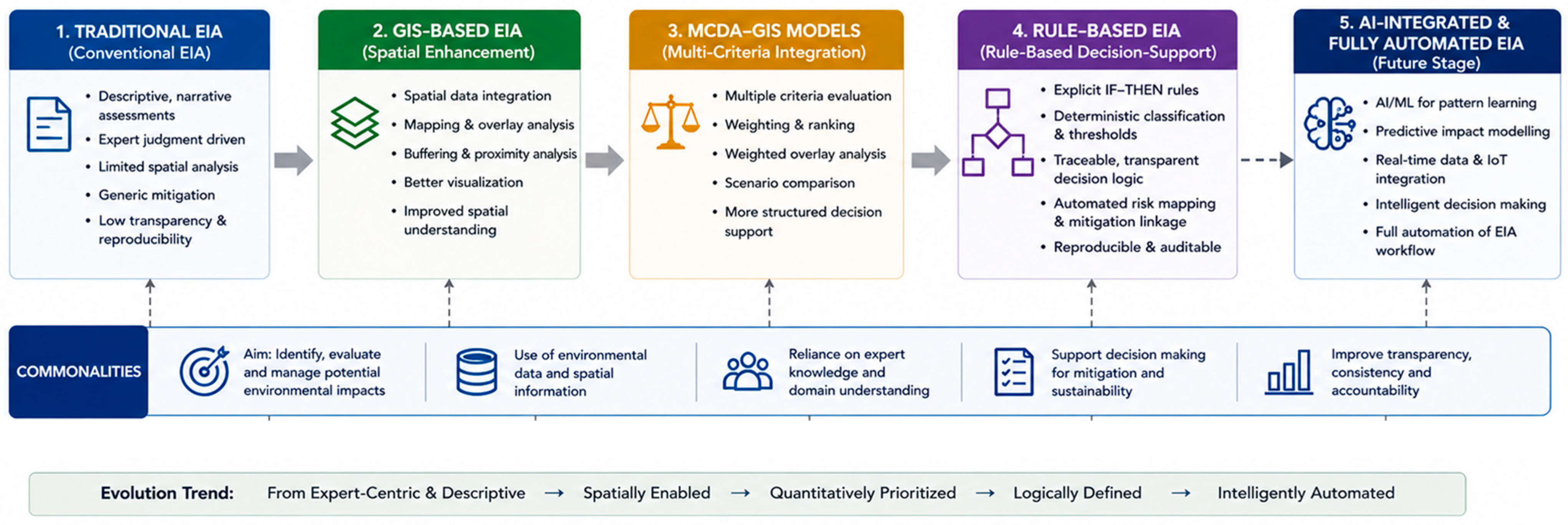Figure 1 compares conventional EIA, GIS-based EIA, MCDA–GIS models and rule-based decision-support models, showing their commonalities and interlinkage.

This shows that despite the growing use of GIS and MCDA in environmental assessment, existing approaches remain limited in three key aspects: (1) the lack of formalized impact ontology linking receptors, impacts, and mitigation within a unified structure; (2) the absence of rule-based computational logic enabling reproducible and automated risk classification; and (3) the limited integration of lifecycle-sensitive and comparative assessment within a single platform. Thus, this study addresses these gaps by developing a structured rule-based decision-support system that operationalizes EIA logic into a transparent, reproducible, and context-sensitive workflows contributing toward the development of computational environmental intelligence systems. The proposed framework also addresses the lack of standardized EIA reporting and emphasizes receptor-based and phase-to-phase reporting framework in the assessment process.

2. Methodology for Developing the Proposed Framework

The proposed framework adopts a problem-oriented computational environmental assessment strategy integrating six analytical dimensions: spatial interaction, receptor vulnerability, lifecycle sensitivity, contextual environmental conditions, uncertainty propagation, and mitigation prioritization. Rather than evaluating environmental impacts independently, the framework formalizes environmental reasoning through interacting environmental indicators and receptor-sensitive assessment logic. The research methodology includes the following steps: (1) framing the EIA as a structured decision system; (2) variable selection, scaling, normalization, and calibration procedures; (3) GIS and rule-based integration for risk identification and standardized reporting; (4) statistical validation; and (5) developing the architecture of the proposed framework.

The authors used Replit Agent 4 for writing, running, and deploying code directly from a web browser, and ChatGPT 5.5 for the purposes of visualization and supporting mathematical equations.

2.1. Theoretical Framing: EIA as a Structured Decision System

The research method formalizes EIA as a multi-criteria decision problem under spatial uncertainty as shown in Equation (1)—where risk magnitude is a function of project characteristics (P), receptor sensitivity (R), spatial interaction intensity (S), and lifecycle stage (L). It also acknowledges the effect of impact categories (I) and assists in defining mitigation measures (M). Based on that, risk was classified into the following classes, very high, high, moderate, low and very low, corresponding to a relative weight of 1.00, 0.80, 0.60, 0.40 and 0.20, respectively.

Risk_i,j,k = f (P_i,R_j,S_ij,L_k)

(1)

The hierarchical structure of the proposed tool is made up of four interrelated levels: Receptor Domain Layer, Impact Mechanism Layer, Risk Characterization Layer, and Mitigation Layer. The former identifies receptor groups that reflect the environmental and social elements that may be influenced by the proposed development, including human health, air environment, natural resources, terrestrial and aquatic ecosystems, and climate-related factors. This is a systematic data entry of impact analysis receptor-based organization that conforms to the best practice of EIA [2]. The second tier includes impact categorization to the defined receptor groups, including noise, air emissions, water pollution, land degradation and biodiversity disturbance. The third includes listing risks, which entails identifying site-specific hazards occurring due to the interaction of projects and their surroundings. These risks are measured on severity and likelihood bases (severity × likelihood matrix), following the work of previous studies [16]. Mitigation measures are the fourth level that includes pre-defined responses that directly refer to particular risks and impact categories. Noting that environmental risk is spatially contingent, spatial interaction intensity is defined as shown in Equation (2):

$$S_{ij}=f(D_{ij},O_{ij},C_{ij},L_k,R_j,U_t)$$

(2)

where $D_{ij}$: proximity interaction, $O_{ij}$: spatial overlap intensity, $C_{ij}$: contextual sensitivity, $L_k$: lifecycle modifier, $R_j$: receptor vulnerability, and $U_t$: uncertainty-adjusted weighting.

2.2. Variable Selection, Scaling, Normalization, and Calibration Procedures

Because the proposed framework integrates heterogeneous environmental datasets with different units, spatial resolutions, and measurement scales, all variables were normalized to a dimensionless range between 0 and 1 prior to risk computation to enable consistent comparison and weighted integration within the rule-based assessment model—following Equation (3) and

Table 1. Variables, units, and scaling structure.

Variable	Symbol	Unit	Original Range	Normalized Range	Description
Receptor proximity distance	Dij	metres	0–15,000 m	0–1	Distance between airport activity zone and receptor
Spatial overlap ratio	Oij	percentage (%)	0–100%	0–1	Degree of overlap between operational buffers and receptors
Population density	Pdens	persons/km2	0–35,000	0–1	Population exposure intensity
Ecological sensitivity	Ecj	ordinal scale	1–5	0–1	Relative ecological vulnerability
Operational intensity	Opi	flights/day	0–950	0–1	Airport operational pressure
Lifecycle severity modifier	Lk	ordinal scale	1–5	0–1	Phase-related impact intensity

.

$$X_{norm}={\displaystyle \frac{X_i-X_{min}}{X_{max}-X_{min}}}$$

(3)

where $X_i$ = observed variable value, $X_{min}$ = minimum dataset value, and $X_{max}$ = maximum dataset value.

Then, the weighting coefficients were initially calibrated using a combination of Egyptian environmental regulations, international airport environmental assessment guidelines, and threshold ranges identified in relevant EIA and GIS risk assessment [6,19,31]. The calibration process focused on three principal criteria: (1) spatial interaction calibration, (2) risk threshold classification criteria, and (3) proposed severity calibration table.

The former established explicit threshold values for the principal listed variables. Thus, the distance weight (${\mathrm{w}}_{\mathrm{d}}$), representing the proximity sensitivity importance, the overlap weight (${\mathrm{w}}_{\mathrm{o}}$) representing the spatial exposure intensity, and the context sensitivity weight (${\mathrm{w}}_{\mathrm{c}}$), representing the environmental vulnerability weighting, lifecycle modifier ${(w}_l)$, receptor vulnerability $\left(w_r\right)$, and uncertainty adjustment ${(w}_u)$, are assigned values of 0.25, 0.20, 0.20, 0.10, 0.15, and 0.10, respectively. The weighting structures are commonly established through expert-informed calibration, environmental interaction logic, and sensitivity evaluation [31,32,33].

For the second calibration criteria, the framework classified environmental risk using a composite severity–likelihood structure. Both the severity and likelihood were evaluated on a five-level ordinal scale ranging from 1 (Very Low) to 5 (Very High), as shown in

Table 2. Severity–likelihood risk matrix used in the rule-based model.

Severity\Likelihood	1 Very Low	2 Low	3 Moderate	4 High	5 Very High	Significance
1 Very Low	1	2	3	4	5	Negligible localized effect
2 Low	2	4	6	8	10	Minor short-term effect
3 Moderate	3	6	9	12	15	Noticeable but manageable impact
4 High	4	8	12	16	20	Significant environmental disruption
5 Very High	5	10	15	20	25	Severe cumulative or persistent impact

. Aggregate risk scores were subsequently categorized into Low-, Moderate-, and High-risk classes according to predefined threshold ranges, as shown in

Table 3. Spatial interaction thresholds and risk classification criteria.

Parameter	Classification	Threshold Range [31,32,33]	Interpretation
Spatial Interaction Intensity (Sij)	Low	<0.35	Limited receptor interaction
	Moderate	0.35–0.75	Partial receptor overlap
	High	>0.75	Extensive receptor exposure
Receptor Sensitivity	Low	Sparse or non-sensitive land use	Minimal environmental vulnerability
	Moderate	Mixed-use or transitional receptors	Moderate environmental sensitivity
	High	Dense population/ecological protection zones	High environmental vulnerability
Operational Intensity	Low	Limited operational frequency	Reduced environmental pressure
	Moderate	Medium operational activity	Moderate environmental load
	High	Continuous high-capacity operations	Persistent environmental exposure
Aggregate risk score	Low	1–5	Limited environmental significance
	Moderate	6–12	Requires mitigation and monitoring
	High	13–25	Significant environmental impact requiring priority mitigation

. It is noted that risk is evaluated separately for each project phase, including construction and operation. This lifecycle differentiation allows for the detection of cumulative versus transitional impacts. Finally, mitigation responses are conditionally linked to risk classification and receptor type, as shown in Equation (4). This ensures mitigation traceability and prevents generic recommendations.

M_i,j,k = g (Risk_i,j,k, Receptor_j)

(4)

2.3. GIS and Rule-Based Integration for Risk Identification and Standardized Reporting

GIS is used to depict the environmental context as layered spatial datasets. The database was developed using multi-source spatial datasets representing environmental receptors, land-use and land-cover conditions, ecological sensitivity and protected-areas, hydrological and flood-risk zones, and operational exposure zones surrounding the airport case study projects. The spatial boundaries of the project are defined with georeferenced polygons, and spatial operations like overlay, buffering, and proximity analysis. These are used to determine the interactions between the project site and the environmental receptors around it. Such spatial relationships allow for context-specific risk identification and mitigation proposal. Also, project-level attributes included passenger capacity, operational frequency and development stage are added as input layers. GIS-derived interactions and project properties are transformed into structured assessment results using rule-based reasoning. This is done by decision rules that relate spatial overlaps, project type and lifecycle stage to a set of predefined risk levels and mitigation requirements.

All spatial datasets were normalized to a unified coordinate reference system and resolution as shown in

Table 4. Spatial datasets and GIS preprocessing workflow.

Spatial Dataset	Source	Year	Format	Resolution/Scale	Coordinate Reference System	Main Pre-Processing Steps
Land Use/Land Cover	Egyptian Survey Authority [34] and Sentinel-derived classification [35]	2024	Raster	30 m	WGS84/UTM 36N	Reclassification, clipping, normalization
Population Density	WorldPop [36]/CAPMAS estimates [37]	2024	Raster	100 m resampled to 30 m	WGS84/UTM 36N	Resampling, density normalization
Ecological Sensitivity Zones	EEAA protected areas database [38]	2024	Vector polygon	1:25,000	WGS84/UTM 36N	Topology correction, overlay preparation
Hydrological Risk Zones	Egyptian Hydrological Authority datasets [39]	2023	Vector polygon	1:50,000	WGS84/UTM 36N	Flood-zone classification, clipping
Airport Operational Boundaries	Airport planning documents [40]	2024	Vector polygon	Project scale	WGS84/UTM 36N	Boundary harmonization
Noise Exposure Buffers	Generated within GIS model	2024	Vector buffer	Multi-distance buffers	WGS84/UTM 36N	Buffer generation and receptor overlap analysis

. Thus, datasets were projected to the WGS 84/UTM Zone 36N coordinate reference system (EPSG:32636), which is commonly adopted for national-scale spatial analysis in Egypt [19]. Raster datasets were resampled to a consistent spatial resolution of 30 m, while vector layers were topologically cleaned and clipped to the defined airport influence zones.

2.4. Statistical Analysis

To ensure methodological robustness and reproducibility, the proposed framework was subjected to a multi-layer validation protocol. The objective was to assess whether the model outputs remain stable, interpretable, and discriminative under plausible variations in input parameters and spatial weighting assumptions.

To assess output stability under parameter uncertainty, a Monte Carlo simulation was performed using Python version 3.14.5 statistical libraries (NumPy and SciPy) integrated with the GIS analytical workflow [41]. This followed Equation (5), with the number of iterations n = 10,000 for better model stability—following previous research [29]. Input weights were sampled from truncated normal distributions, with the coefficient of variation set at ±15% range relative as shown in

Table 5. Baseline parameters used in Monte Carlo simulation.

Parameter	Symbol	Baseline Mean (${\mathit{\mu }}_{\mathit{i}}$)	Standard Deviation (${\mathit{\sigma }}_{\mathit{i}}$)	Distribution Type	Perturbation Range	Functional Role
Distance interaction weight	$w_d$	0.25	0.0375	Truncated normal	±15%	Controls proximity-based environmental exposure
Spatial overlap weight	$w_o$	0.20	0.0300	Truncated normal	±15%	Represents cumulative overlap intensity
Context sensitivity weight	$w_c$	0.20	0.0300	Truncated normal	±15%	Represents environmental vulnerability amplification
Lifecycle modifier weight	$w_l$	0.10	0.0150	Truncated normal	±15%	Represents phase-sensitive impact intensity
Receptor vulnerability weight	$w_r$	0.15	0.0225	Truncated normal	±15%	Represents receptor resilience and sensitivity
Uncertainty adjustment weight	$w_u$	0.10	0.0150	Truncated normal	±15%	Represents uncertainty stabilization and robustness adjustment

—which is academically accepted [29]. This perturbation range was selected to represent moderate uncertainty associated with expert-calibrated spatial weighting, receptor sensitivity estimation, and operational intensity assumptions in GIS-supported environmental assessment models.

Calculating uncertainty propagation followed Equation (6), where ${\mu }_i$ represents the calibrated baseline parameter value, and ${\sigma }_i$ represents standard deviation. Robustness evaluation using the 95% confidence interval was computed following Equation (7).

$$w_i\sim N({\mu }_i,{\sigma }_i^2)$$

(5)

$$CV={\displaystyle \frac{\sigma }{\mu }}$$

(6)

$$C{I}_{95}=\mu \pm 1.96\sigma$$

(7)

The simulation outputs demonstrated relatively stable aggregate risk distributions across the three airport cases. Mean risk values remained within narrow confidence intervals despite moderate perturbation of weighting parameters.

2.5. Developing the Architecture of the Proposed Framework

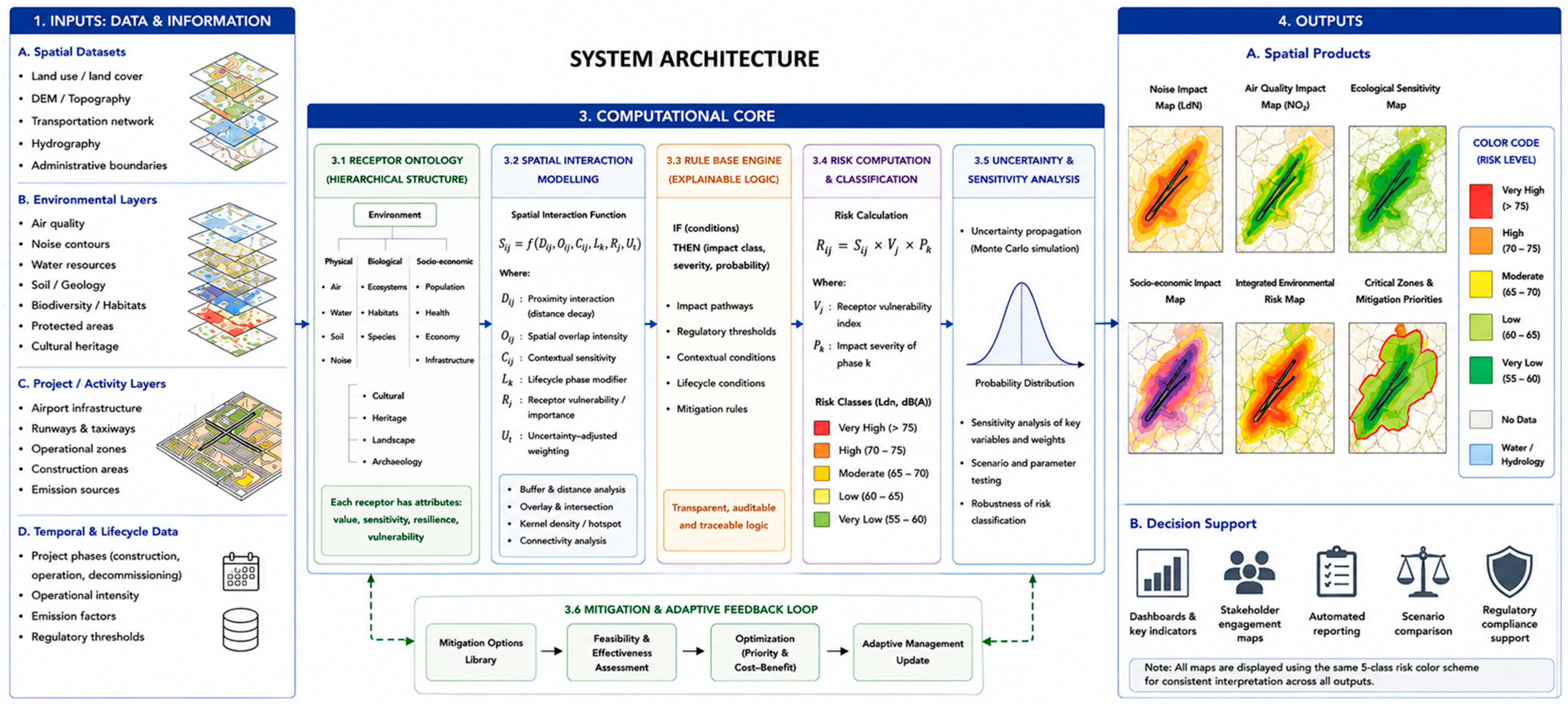
The proposed system architecture constitutes (1) inputs including spatial datasets, environmental layers, receptors and lifecycle conditions; (2) computational core including rule engine, spatial interaction function, risk computation and uncertainty propagation; and (3) outputs including risk maps, critical zones, mitigation priorities and decision-support dashboards—as shown in Figure 2. It operates through hierarchical features for the receptors, impact categories, risks, and mitigation measures, and allows automatically gathering the results of the assessment into a unified format consistent with formal EIA reporting requirements. Every report combines the description of the project, its spatial background, GIS-based risks, the impact of the project evaluated by the lifecycle, and the proposed mitigation measures. The proposed framework can be found at the following hyperlink https://66918e9f-d8bf-439a-a0f3-a233f519457c-00-2tobyacwd4dw0.spock.replit.dev/ accessed on 1 April 2026, in addition to the Supplementary Materials.

3. Case Study Application

3.1. Case Study Description

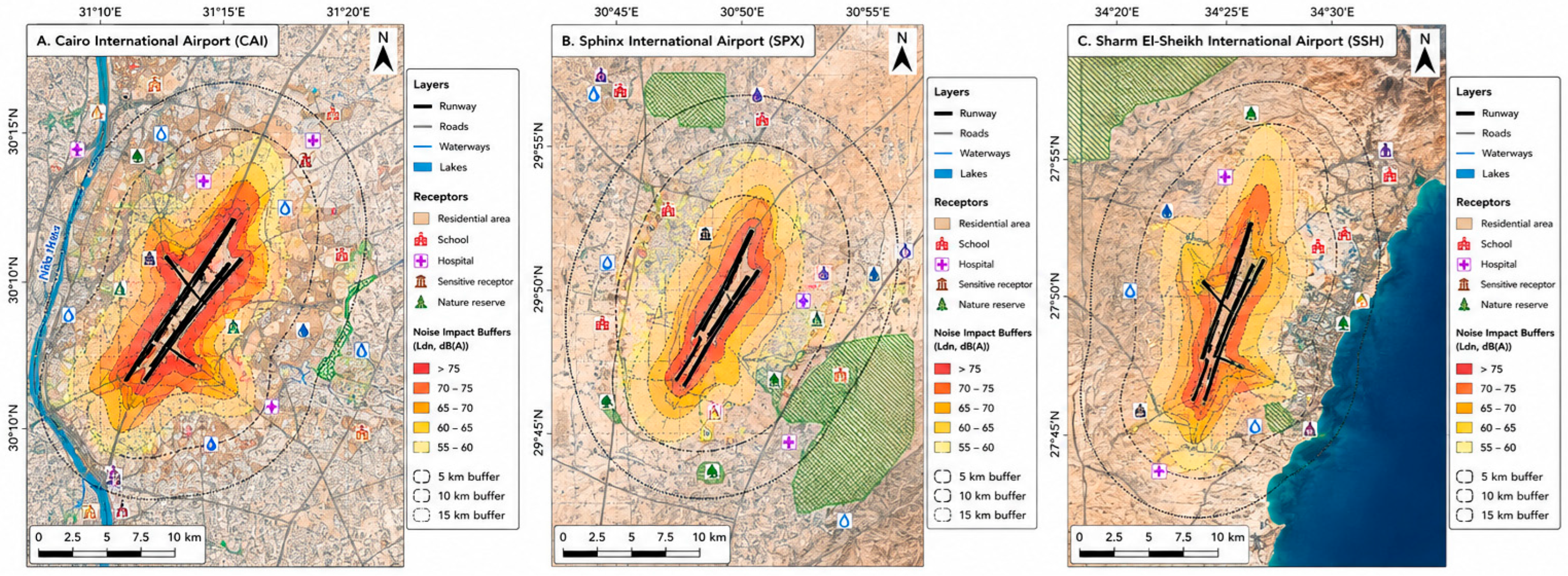
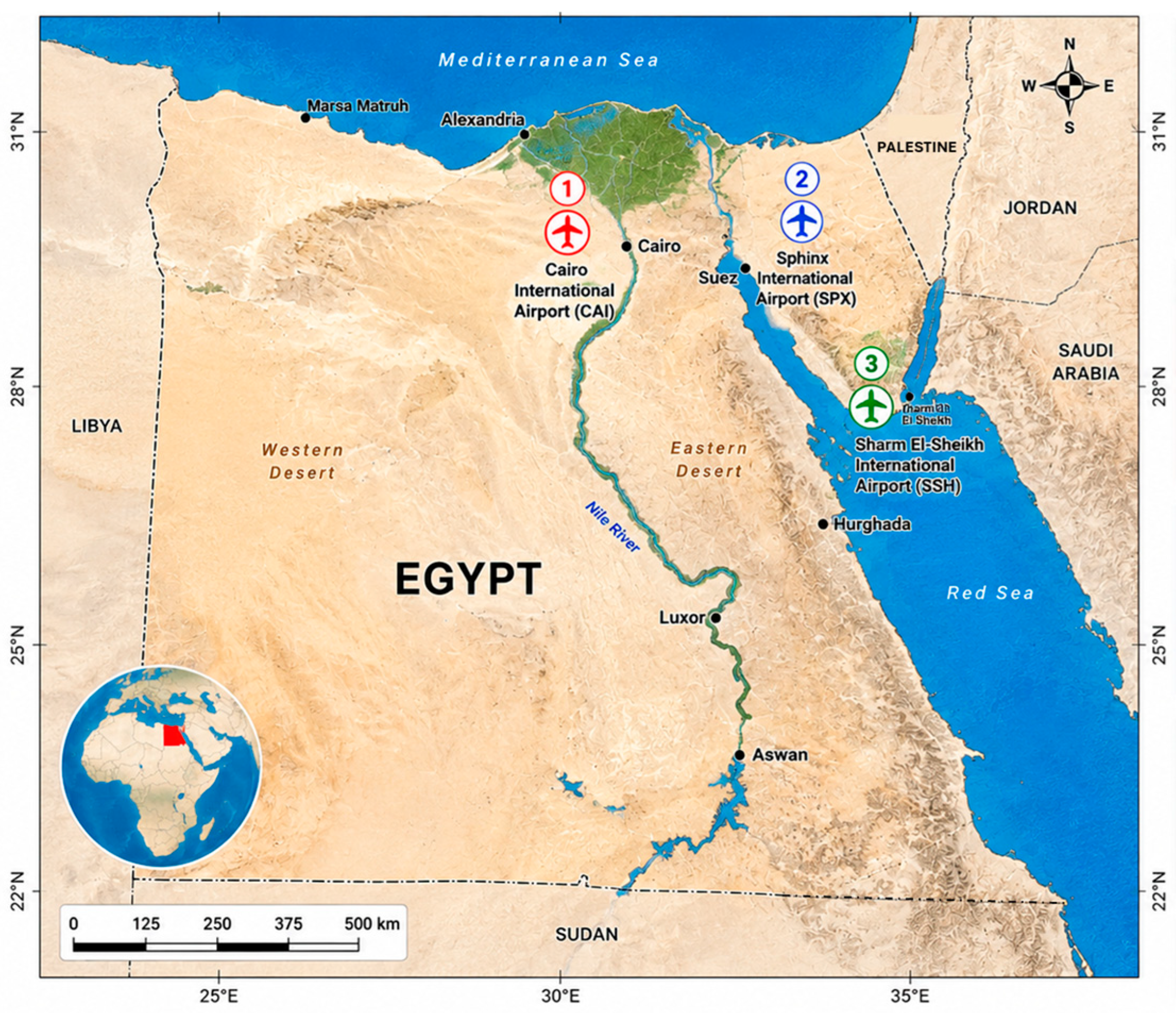
The framework was applied to three airport projects in Egypt, as shown in Figure 3, which were intentionally selected through a purposive comparative sampling strategy to represent distinct spatial–environmental typologies that commonly shape airport-related environmental impact profiles in Egypt. These represent differentiated spatial typologies: dense urban environment, peripheral low-density expansion zone and coastal tourism–ecological environment. Together, these cases provide variation in urban form, receptor structure, operational intensity, and environmental sensitivity, allowing the framework to be tested under contrasting spatial conditions. This allows for the structural validation of the proposed framework adaptability.

Cairo International Airport (CAI) has the greatest environmental impact, owing to its scale of operations and being in a dense urban fabric. It has been recorded that air pollutant emissions and noise exposure are high in perennial landing and take-off procedures, ground support operations, and traffic jams in the nearby residential neighbourhoods. Applying the proposed tool indicates that the expected environmental impacts reach the sensitive population receptors; which causes the severity of risks to be high during the operational stage. The hierarchical receptor-based framework allows for systematic grouping of risks whereas rule-based decision-support systems relate them with specific mitigation options like the deployment of ground power units, constraints on auxiliary power units, and operational noise management. This case exhibits how EIA Maps can be used to accommodate cumulative impact analysis in high-density urban settings.

The environmental profile of the Sphinx International Airport (SPX) is different, owing to its low current operational intensity and minimal effect on sensitive areas, as the location is at the periphery of the desert. According to current measurements, the levels of noise and emissions are below the national environmental standards, but future growth is likely to create new environmental loads. The proposed tool indicates that SPX currently poses low-to-moderate environmental risk. The tool offers future scenario-based assessment associated with emerging risks in air quality, noise, and land-use receptors. The phase-oriented assessment indicates the role of early mitigation planning and environmental monitoring and shows how spatial empowerment tools can be used in promoting proactive environmental management during the development of the project.

Sharm El-Sheikh International Airport (SSH) environmental performance is highly affected by the seasonal tourism demand and its location in close proximity to coastal and resort-sensitive environments. Past research demonstrates that environmental pressures caused by SSH are highly variable, associated with the peaks of the tourism seasons, noise and emissions have increased temporarily instead of being exposed constantly. Using the proposed tool, GIS based analysis identifies spatial sensitivity in the coastal ecosystems and tourism land uses during building operation. These risks are associated with their corresponding adaptive mitigation strategies, which are: flight scheduling controls, optimized ground operations, and continuous environmental monitoring. This project underscores the significance of time sensitive assessment logic and dynamism and reveals how standard-based digital EIA tools can address temporal variability in environmentally sensitive areas.

Table 6. Comparative environmental risk validation across the three airport case studies.

Airport	Spatial Context	Dominant Receptors	Dominant Lifecycle Phase	Risk Severity ClassifiCation	GIS Spatial Evidence	Threshold Condition Triggered
CAI (706.3 km2)	Dense urban metropolitan context	Population density, air quality, noise-sensitive land uses	Operation phase	High cumulative risk	Extensive overlap between operational buffers and high-density residential zones Strong proximity to sensitive population receptors	High receptor proximity High operational intensity Continuous exposure
SPX (668.9 km2)	Peri-urban/desert expansion zone	Future population growth areas, land resources	Future operational expansion phase	Low–Moderate risk	Limited current overlap with sensitive receptors Spatial exposure concentrated around projected urban growth corridors	Moderate spatial interaction Projected growth scenarios
SSH (482.7 km2)	Coastal tourism-ecological context	Coastal ecosystems, tourism land use, sensitive ecological zones	Seasonal operation phase	Moderate but temporally variable risk	Spatial proximity to coastal ecological systems and tourism-related receptors with seasonally fluctuating operational exposure	Ecological sensitivity Seasonal operational peaks

summarizes the environmental risk profiles for the three case study projects. Also, Figure 4 shows GIS spatial layers, buffer and critical zones for environmental risk assessment.

3.2. Case Study Computations

Step 1: Normalizing environmental variables are shown in

Table 7. Normalizing environmental variables for the three case studies.

Variable	CAI		SPX		SSH
	Value	Justification	Value	Justification	Value	Justification
${\mathit{D}}_{\mathit{i}\mathit{j}}$	0.82	Strong urban receptor proximity	0.65	Lower receptor proximity	0.60	Lower urban proximity
${\mathit{O}}_{\mathit{i}\mathit{j}}$	0.78	High overlap with residential and infrastructure zones	0.70	Moderate overlap pattern	0.62	Narrower interaction footprint
${\mathit{C}}_{\mathit{i}\mathit{j}}$	0.68	Moderate contextual sensitivity	0.58	Moderate contextual sensitivity	0.92	Very high ecological sensitivity
${\mathit{L}}_{\mathit{k}}$	0.90	High operational lifecycle intensity	0.72	Expansion-phase activity	0.75	Tourism-driven operational pressure
${\mathit{R}}_{\mathit{j}}$	0.88	Dense population vulnerability	0.60	Lower receptor density	0.86	Sensitive ecological receptors
${\mathit{U}}_{\mathit{t}}$	0.80	Moderate uncertainty stability	0.78	Moderate uncertainty variability	0.82	Stable uncertainty response

. The weighting was established through expert-informed calibration, environmental interaction logic, and sensitivity evaluation following previous studies [31,32,33].

Step 2: Deriving spatial interaction intensity ($S_{ij}$) for each case study using the spatial-risk distributions, and their corresponding risk classification weights (0.25, 0.20, 0.20, 0.10, 0.15, 0.10)

$$\begin{gathered} S_{CAI}=\left(0.25\times 0.82\right)+\left(0.20\times 0.78\right)+\left(0.20\times 0.68\right)+\left(0.10\times 0.90\right)+ \\ (0.15\times 0.88)+(0.10\times 0.80)=0.799\left(\mathrm{High}\right) \end{gathered}$$

$$\begin{gathered} S_{SPX}=(0.25\times 0.65)+(0.20\times 0.70)+(0.20\times 0.58)+(0.10\times 0.72)+ \\ (0.15\times 0.60)+(0.10\times 0.78)=0.659\left(\mathrm{Moderate}\text{-}\mathrm{High}\right) \end{gathered}$$

$$\begin{gathered} S_{SSH}=(0.25\times 0.60)+(0.20\times 0.62)+(0.20\times 0.92)+(0.10\times 0.75)+ \\ (0.15\times 0.86)+(0.10\times 0.82)=0.744\left(\mathrm{High}\right) \end{gathered}$$

Step 3: Assigning Remaining Parameters

Impact intensity, receptor sensitivity, and lifecycle modifier (operation phase)—these were determined on a range of (0–1)- as shown in

Table 8. Computing impact intensity, receptor sensitivity, and lifecycle modifier for each case study project.

Airport	${\mathit{P}}_{\mathit{i}}$ Impact Intensity	${\mathit{R}}_{\mathit{j}}$ Receptor Sensitivity	${\mathit{L}}_{\mathit{k}}$ Lifecycle Modifier (Operation Phase)
CAI	0.90	0.85	1.00
SPX	0.75	0.70	1.00
SSH	0.80	0.95	1.00

based on the situation of each case study (airport scale, traffic intensity, operational continuity, receptor exposure persistence, and environmental sensitivity). The weighting structures are based on expert-informed calibration, environmental interaction logic, and sensitivity evaluation, following previous studies [31,32,33].

Step 4: Final Risk Calculation

$$Ris{k}_{CAI}=0.90\times 0.88\times 0.799\times 0.90=0.570\left(\mathit{High}\mathit{\right)}$$

$$Ris{k}_{SPX}=0.75\times 0.60\times 0.659\times 0.72=0.214\left(Moderate\right)$$

$$Ris{k}_{SSH}=0.80\times 0.86\times 0.744\times 0.75=0.384\left(Moderate\text{-}high\right)$$

Step 4. Mitigation Intensity Computation—the given receptor weighting for the population and health, ecological systems and hydrological systems, corresponding to values of 1.00, 1.20 and 1.10, respectively. The weighting structures are established through expert-informed calibration, environmental interaction logic, and sensitivity evaluation [31,32,33].

3.3. Case Study Statistical Validation

To test whether the model meaningfully differentiates spatial contexts, inter-case variance was compared against intra-case uncertainty variance following Equation (8).

Let:

η = Var_between/Var_within

(8)

where Var_between is the variance of mean risk across airports, and Var_within is the average Monte Carlo variance within each airport.

Spearman’s rank correlation coefficient (ρ) was calculated using SPSS version 31.0.2.0 [42] between baseline ranking and each Monte Carlo iteration following Equation (9). The analysis was conducted for different project phases (construction and operation), and for different impact categories independently to assess whether lifecycle differentiation remained stable under parameter uncertainty. It is noteworthy that the classification stability remained within acceptable variation ranges across all simulations.

ρ = 1 − 6∑d_i²/n(n² − 1)

(9)

where ρ is Spearman’s rank correlation coefficient, d represents the difference between the two ranks of each observation, and n represents the number of observations.

Furthermore, to evaluate agreement between the model-generated environmental classifications and regulatory environmental thresholds, Cohen’s Kappa statistic ($\kappa$) was calculated using SPSS [42] for the principal impact categories including noise exposure, air quality impact, and ecological sensitivity. The comparison was conducted using rasterized spatial analysis units derived from GIS overlay operations. The study area surrounding each airport was subdivided into standardized 30 m × 30 m spatial grid cells corresponding to the normalized raster resolution used throughout the analysis framework. Each spatial unit was independently classified according to the model-generated environmental risk classification and regulatory compliance/exceedance classification into: Compliant (0)—Environmental indicator remained below regulatory threshold, and Non-Compliant/Exceedance (1)—Environmental indicator exceeded regulatory threshold. Similarly, the model-generated outputs were binarized according to the calibrated rule-based risk thresholds: Low/Moderate Risk—Compliant (0), and High Risk—Non-Compliant/Exceedance (1). Agreement interpretation followed the classification guidance proposed by previous scholars [31,32,33].

Observed agreement ($P_o$) and expected agreement ($P_e$) were computed using Equation (10):

$$\kappa ={\displaystyle \frac{P_o-P_e}{1-P_e}}$$

(10)

4. Results and Discussion

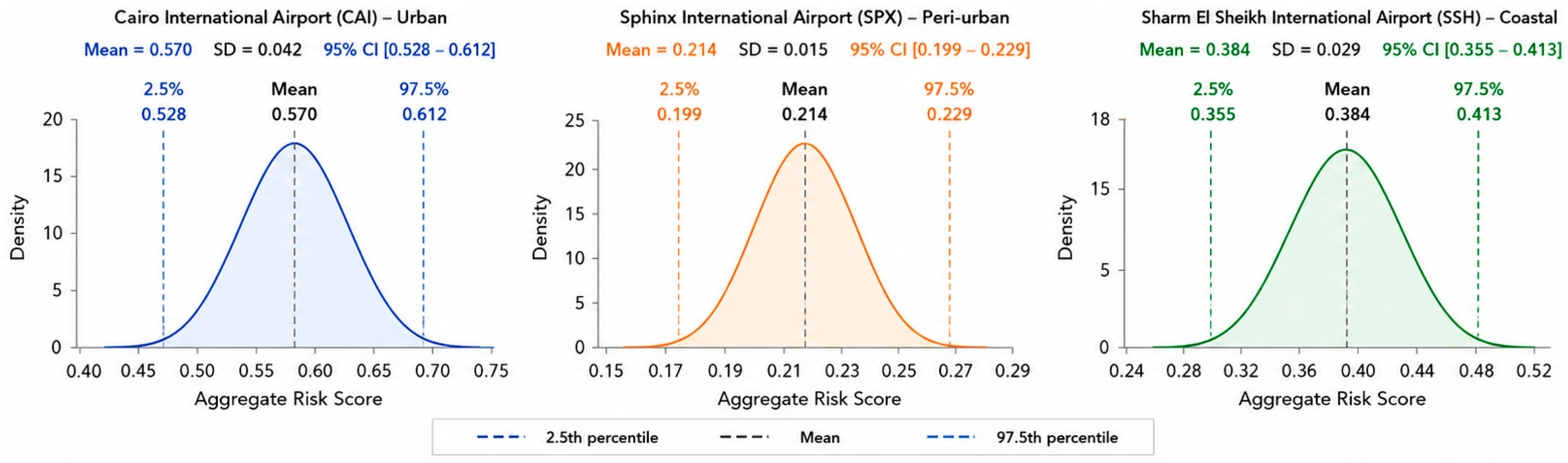
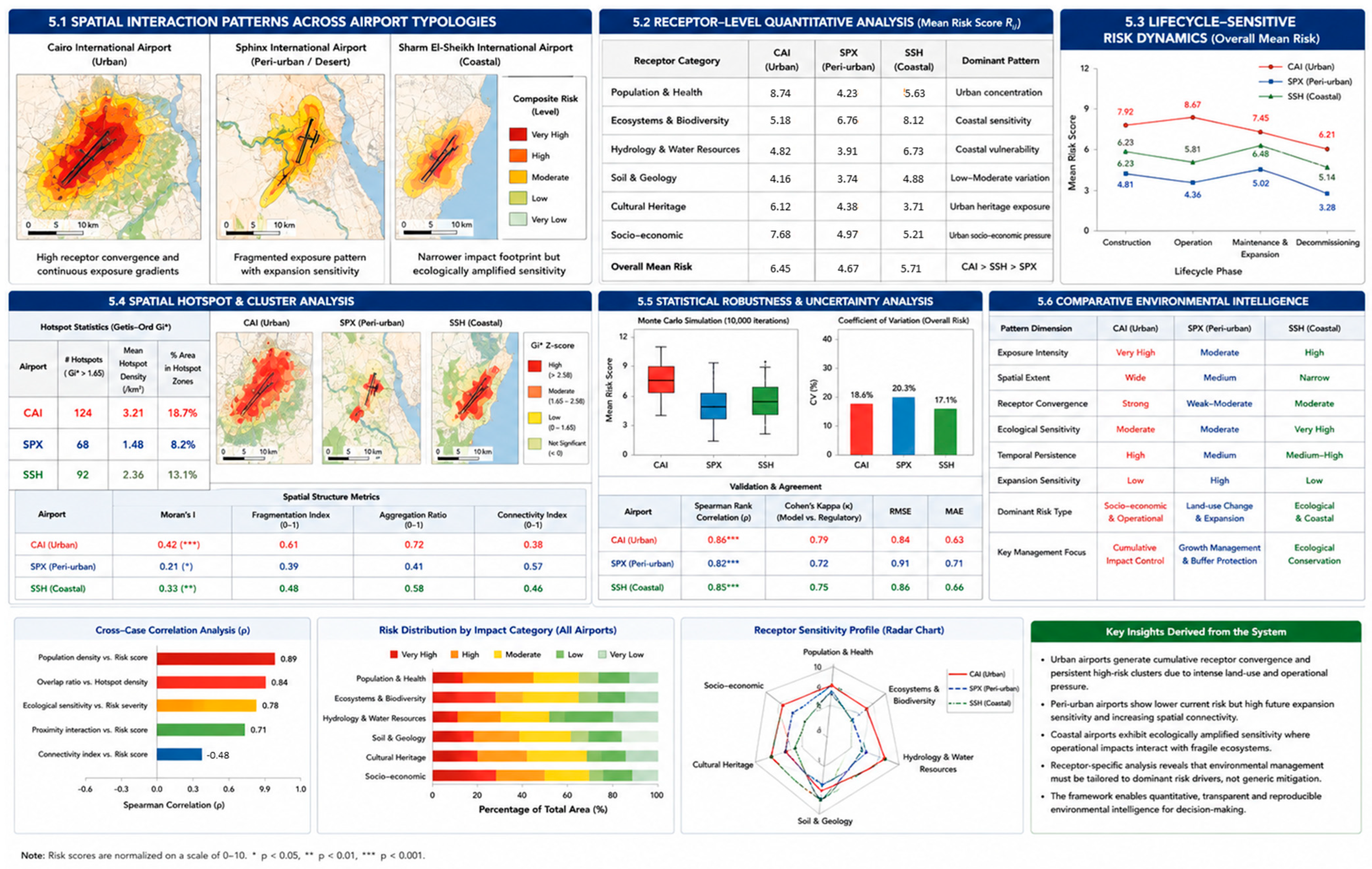
The resulting distribution of risk scores across the three case studies—shown in Figure 5 and

Table 9. Integrated comparative results for uncertainty propagation.

Airport	${\mathit{S}}_{\mathit{i}\mathit{j}}$	Risk Score	Monte Carlo Mean	Standard Deviation	Ecological Mitigation	95% Confidence Interval	Coefficient of Variation (%)	Dominant Environmental Pattern
CAI	0.799	0.570	0.828	0.042	0.684	0.528–0.612	7.4	Urban receptor convergence
SPX	0.659	0.214	0.650	0.015	0.257	0.199–0.229	6.8	Transitional peri-urban expansion
SSH	0.744	0.384	0.772	0.029	0.461	0.355–0.413	7.5	Ecological sensitivity amplification

—allowed for an estimation of the mean risk, standard deviation, 95% confidence intervals and probability of rank inversion across cases. Across simulations, no rank reversal occurred between the three airport case studies. The resultant mean ρ = 0.96 (p < 0.001) indicates near-perfect rank stability across parameter perturbations. This confirms that classification outcomes are not sensitive to moderate calibration shifts. The coefficient of variation for aggregate risk remained below 8% in all cases, and the sensitivity analysis demonstrated that moderate variation (±15%) in spatial weighting coefficients did not alter ordinal risk ranking across cases, indicating strong output stability under moderate parameter uncertainty. Furthermore, the resulting η = 4.73, indicating that between-case differences are nearly five times larger than uncertainty-driven variance. This supports discriminant validity and confirms that case differentiation reflects structural spatial conditions.

The spatial analysis showed definite variations in the distribution of environmental risks in the three airports. CAI demonstrated the highest spatial interaction intensity, the highest aggregate environmental risk. This reflects cumulative urban receptor convergence, continuous operational intensity, and strong overlap with population-sensitive zones. SPX exhibited moderate interaction intensity, lower receptor vulnerability, and lower aggregate environmental risk. It demonstrates fragmented peri-urban exposure patterns and lower cumulative receptor density, but increasing future expansion sensitivity. SSH demonstrated elevated ecological sensitivity, strong vulnerability amplification, and moderate–high aggregate environmental risk. Although urban exposure was lower than CAI, ecological receptor vulnerability significantly increased interaction severity. This integrated computational result demonstrate that environmental risk is not governed solely by airport size or operational scale, but by the interaction between receptor concentration, spatial overlap intensity, contextual sensitivity, and lifecycle conditions. Urban systems generated cumulative receptor convergence, while coastal systems demonstrated vulnerability amplification through ecological sensitivity.

The phase-based evaluation demonstrated that environmental risk profiles varied in accordance with lifecycle differentiation. In all three airports, the operation phase always produced the most cumulative environmental risks, especially aircraft noise, air emissions, and traffic-related effects (the highest aggregate risk score). The risks associated with the construction phase were spatially localized and rated as medium, as they were mostly related to temporary emissions, noise, and soil disturbance. These effects were localized and time-sensitive and hence, their overall severity was less than that of the operational risks.

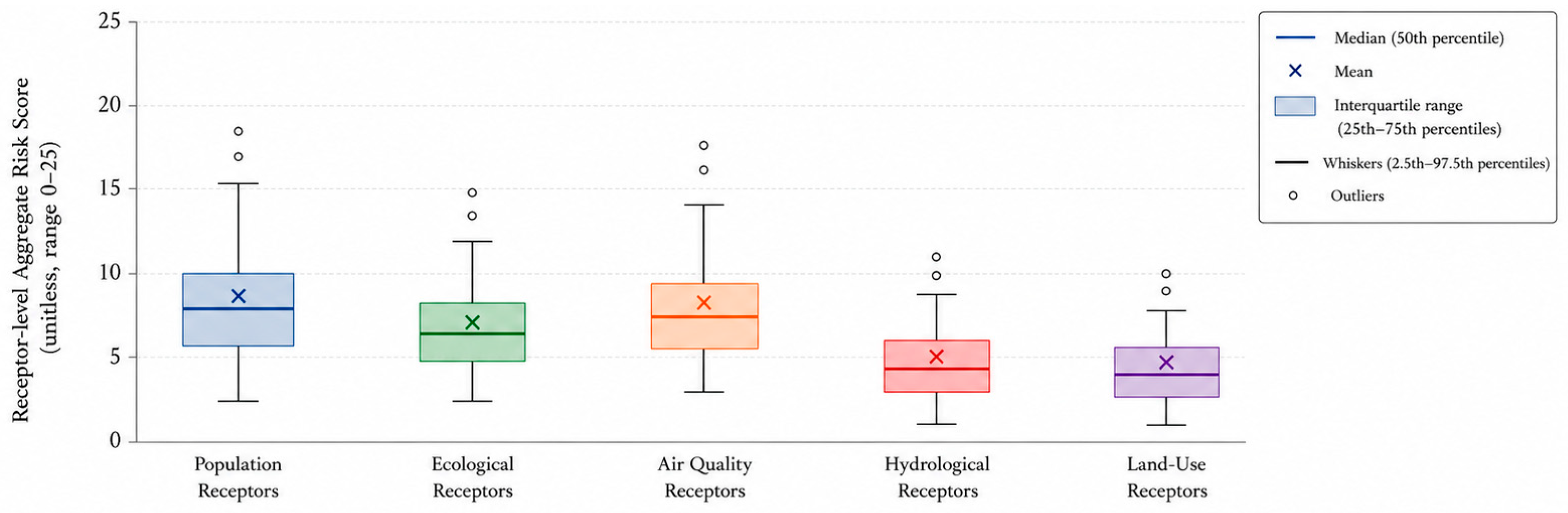
The hierarchical receptor-based structure allowed the systematic arrangement of environmental risks in all case studies. Environmental receptors were grouped into predesignated categories which involved population, air quality, noise sensitive land use, ecological systems, soil and water resources, as shown in Figure 6. The risks identified were then projected to particular categories of impacts and the level of severity through spatial interaction and project characteristics. The existence of such a hierarchical structure enabled the tool to automatically match every identified risk with its associated mitigation measures. Thus, the mitigation actions were thus related to the receptor type, impact severity and project phase. Consequently, mitigation planning became traceable, uniform, and spatially justifiable.

Table 10. Stability assessment for lifecycle-phase and receptor-level risk variability.

		Mean Aggregate Risk	Coefficient of Variation (%)	Classification Stability
Lifecycle Phase	Construction	5.8	7.5	Stable
	Operation	8.7	6.2	Highly stable
Impact categories	Noise	8.9	8.7	Moderate-to-high stability
	Air Emissions	8.1	7.9	High stability
	Runoff/Hydrology	4.9	5.5	High stability
	Land Transformation	5.3	6.1	High stability

shows the stability assessment for lifecycle-phase and receptor-level risk variability.

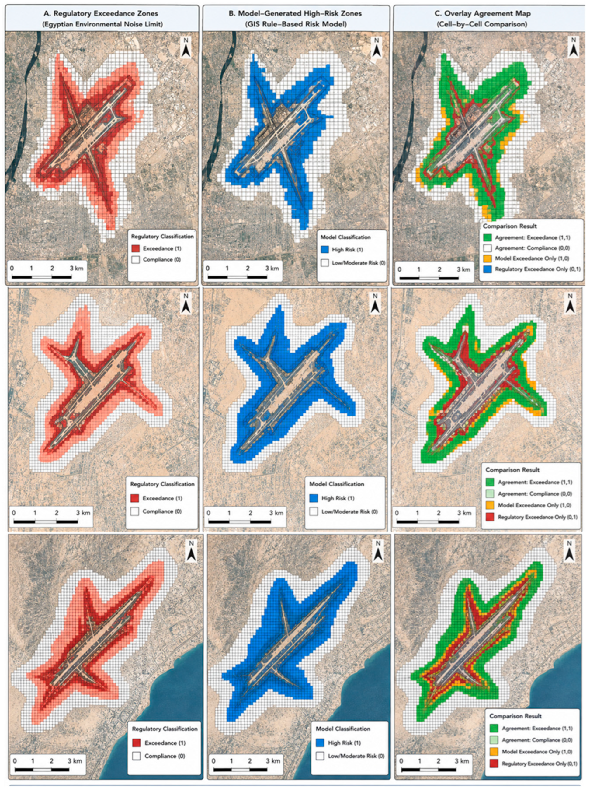
Also, it was found that the Kappa values ranged from 0.71 to 0.79 across impact categories, indicating substantial agreement and confirming the alignment between model classification and regulatory benchmarks. Figure 7 shows the spatial overlay comparison between model-generated exceedance zones and regulatory compliance zones for the three case studies.

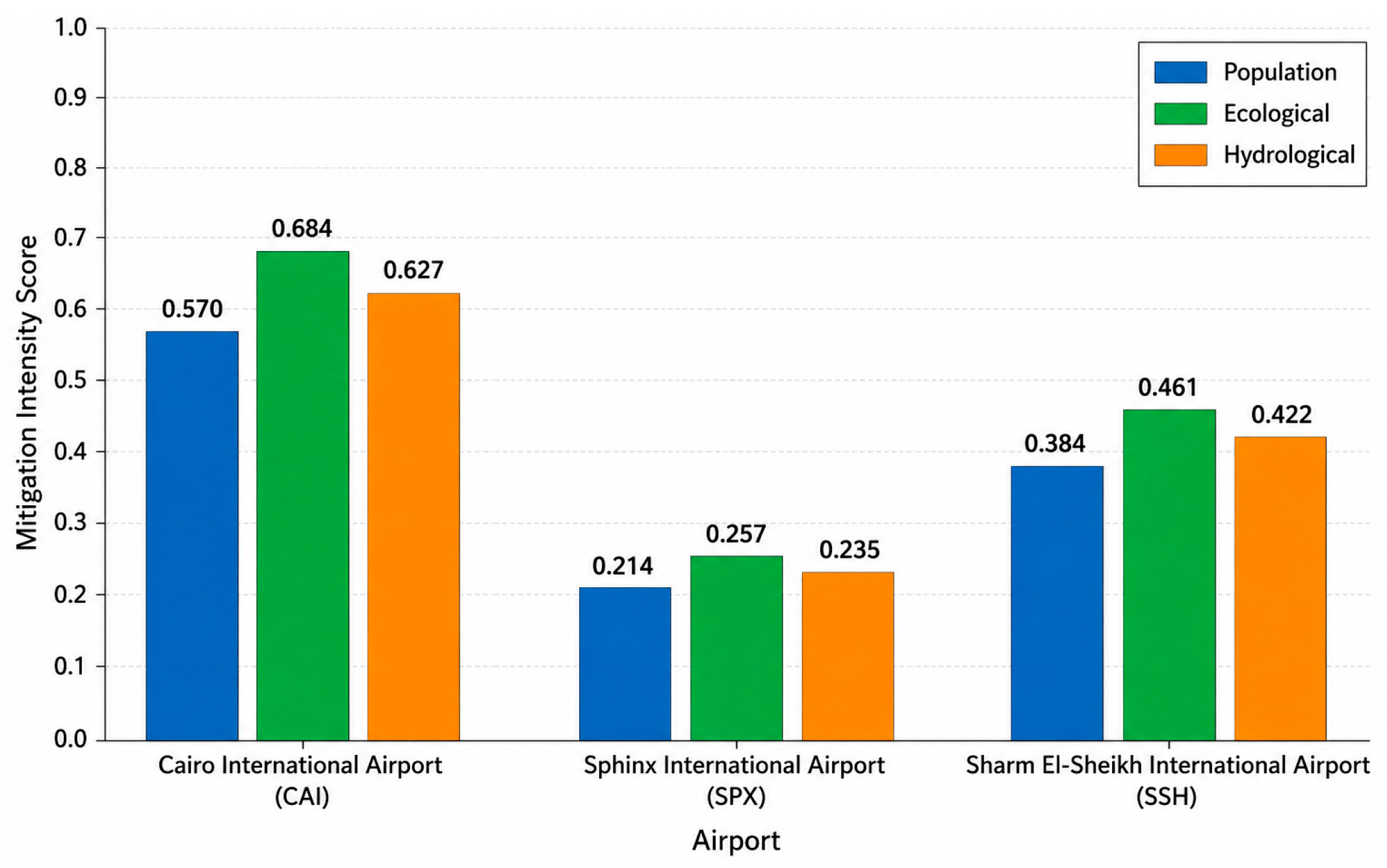
The mitigation intensity for CAI exhibited the highest mitigation requirements across all receptors, with a mitigation score of 0.570 for population receptors, 0.684 for ecological receptors, and 0.627 for hydrological receptors. SPX showed the lowest mitigation requirements among the three case studies, recording mitigation scores of 0.214 for population receptors, 0.257 for ecological receptors, and 0.235 for hydrological receptors. SSH demonstrated intermediate mitigation requirements, with mitigation scores of 0.384 for population receptors, 0.461 for ecological receptors, and 0.422 for hydrological receptors. Across all three airports, ecological receptors consistently produced the highest mitigation requirements as shown in Figure 8, emphasizing the importance of environmentally sensitive receptor protection within the proposed rule-based GIS environmental assessment framework. The full picture describing the proposed framework interface is shown in Figure 9.

Eventually, the findings present a transferable and scalable model that could help improve transparency, consistency, and evidence-based environmental decision-making in Egypt and other developing countries.

Comparison of the findings of this study with relevant studies is shown in

Table 11. Comparing the findings of this study with relevant studies.

Dimension	Proposed Rule-Based GIS Framework	AHP–MCDA-Based EIA [19,43,44]	BIM-Based EIA [11]
Primary objective	Structured spatial decision-support	Multi-criteria prioritization	Digital lifecycle integration
Core logic	Rule-based GIS reasoning	Weighted expert evaluation	Process/model-based assessment
Spatial capability	High GIS interaction modelling	Moderate spatial integration	Limited-to-moderate spatial focus
Expert dependence	Moderate	High	Moderate
Transparency	High traceability and auditability	Moderate transparency	Transparent modelling workflow
Uncertainty treatment	Sensitivity and probabilistic testing	Weight sensitivity testing	Limited/project-specific
Lifecycle integration	Construction and operation	Framework-dependent	Strong BIM lifecycle integration
Mitigation linkage	Direct risk–mitigation mapping	Weighted mitigation prioritization	Coordination-oriented
Automation potential	Semi-automated classification/reporting	Semi-automated evaluation	High information automation
Scalability	Adaptable with GIS data availability	Adaptable but weight-dependent	Dependent on BIM maturity
Main strengths	Explicit spatial/environmental logic	Stakeholder-oriented prioritization	Strong coordination and visualization
Main limitations	Requires high-quality GIS data and calibration	Subjective weighting	Weak environmental causality modelling
Best application context	Spatially sensitive infrastructure EIA	Policy and criteria prioritization	Digitally integrated project management

.

This comparison indicates that while recent digital EIA frameworks have advanced the structuring and management of environmental information, they differ significantly in their underlying decision logic and analytical capabilities [45]. AHP–MCDA frameworks provide strong capabilities for multi-criteria prioritization and stakeholder-informed weighting, while BIM-based EIA approaches offer significant strengths in lifecycle integration, construction coordination, and digital project management. A previous study [16] demonstrates strong integration of risk–mitigation management and automated prioritization through MCDA/AHP techniques; however, it remains dependent on expert-derived weighting schemes and lacks explicit spatial interaction modelling. Another study [11] advances lifecycle integration and digital representation of environmental data but focuses primarily on process optimization and scoring-based evaluation rather than formal decision logic or impact–mitigation traceability.

In contrast, the proposed rule-based GIS decision-support framework introduces a deterministic and spatially explicit approach that formalizes environmental assessment as a reproducible computational process. By explicitly modelling spatial interactions and embedding rule-based logic, the framework reduces subjectivity, enhances transparency, and enables probabilistic risk evaluation, thereby addressing key methodological limitations identified in prior studies.

5. Conclusions and Directions for Future Research

This research aims to enhance the current shortcomings in the practice of EIA, especially the absence of spatial integration, standard classification of impacts, proper decision support systems, and a standardized reporting system. Thus, the study proposed a spatially explicit rule-based EIA-GIS decision-support framework intended to improve the analytical structure, transparency, and reproducibility of EIA practice for complex infrastructure projects. The framework operationalizes EIA through the integration of hierarchical receptor-based classification, GIS spatial interaction analysis, lifecycle-sensitive assessment, and rule-based risk–mitigation logic within a unified computational architecture. This structure enables causal traceability, severity prioritization, cross-project comparability and cumulative assessment potential.

The proposed system architecture constitutes (1) inputs including spatial datasets, environmental layers, receptors and lifecycle conditions; (2) computational core including rule engine, spatial interaction function, risk computation and uncertainty propagation; and (3) outputs including risk maps, critical zones, mitigation priorities and decision-support dashboards. It operates through hierarchical features for the receptors, impact categories, risks, and mitigation measures, and allows automatically gathering the results of the assessment into a unified format consistent with formal EIA reporting requirements. Every report combines the description of the project, its spatial background, GIS-based risks, the impact of the project evaluated by the lifecycle, and the proposed mitigation measures. It is noted that the analytical complexity of the framework is embedded within its multi-dimensional evaluation structure and integrated environmental reasoning architecture, including the following steps:

• Spatial interaction modelling;
• Problem-oriented receptor-based environmental reasoning;
• Comprehensive indicator integration;
• Lifecycle-sensitive assessment;
• Uncertainty-aware environmental computation;
• Comprehensive evaluation architecture.

The study tests the proposed tool to three airport case studies in the same country Egypt (same governing environmental laws and regulations) but in different cities (demonstrating variations in urban context). This revealed clear spatial differentiation in environmental risk profiles across the three case studies. The urban airport exhibited the highest concentration of spatial interactions with sensitive receptors, resulting in elevated cumulative risk levels. The peri-urban case demonstrated lower current risk but increased sensitivity under projected operational expansion. The coastal airport displayed moderate but temporally variable risk patterns driven by seasonal operational intensity and ecological sensitivity.

Validation was conducted using Monte Carlo uncertainty simulation, sensitivity analysis, Spearman’s rank correlation, and Cohen’s Kappa agreement analysis. The resultant mean ρ = 0.96 (p < 0.001) demonstrated stable comparative risk classification across receptor categories, lifecycle phases. The coefficient of variation for aggregate risk remained below 8% in all cases, and the sensitivity analysis indicated moderate variation (±15%) in spatial weighting coefficients, indicating strong output stability under moderate parameter uncertainty. The resulting η = 4.73 supports discriminant validity and confirms that case differentiation reflects structural spatial conditions. Cohen’s Kappa agreement values ranging from 0.71 to 0.79 indicated substantial consistency between model-generated exceedance zones and regulatory environmental classifications. Thus, this comparative application showed that environmental risk profiles varied according to receptor proximity, spatial overlap intensity, operational characteristics, and lifecycle stage. The results further demonstrated that GIS-supported rule-based assessment can support consistent risk classification, mitigation planning, lifecycle-sensitive evaluation, and standardized and comparable reporting outputs across different environmental settings.

Overall, the study presents a potentially transferable framework that helps in bridging regulatory requirements, spatial analysis and practical assessment needs. This helps develop the current EIA practice into a more of a compliance-oriented exercise and more of a structured decision-support system—useful for planners, regulators, and practitioners. It contributes a structured methodological foundation for digitally enabled and spatially informed environmental assessment while highlighting the need for broader empirical validation and operational implementation research. In this regard, the study acknowledges that the efficiency of the proposed rule-based decision-support framework depend greatly on the availability of data, spatial dataset resolution, institutional data accessibility and regulatory alignment with digital workflows. Directions for future research can be by advancing the technical, technological and validation of the model. This is proposed by testing on more case studies with different building typologies and different contextual settings, in addition to incorporating real-time environmental data and more sophisticated machine learning.