Article

Spatiotemporal Variations in Snow/Ice Cover, Climate Responses and Future Trends in the Headwaters of the Keriya River on the Northern Slope of the Kunlun Mountains


1
College of Geography and Remote Sensing Sciences, Xinjiang University, Urumqi 830017, China
2
Xinjiang Key Laboratory of Oasis Ecology, Xinjiang University, Urumqi 830017, China
3
Xinjiang Field Scientific Observation and Research Station for the Oasisization Process in the Hinterland of the Taklamakan Desert, Xinjiang University, Urumqi 830017, China
*
Author to whom correspondence should be addressed.
These authors contributed equally to this work.
Sustainability 2026, 18(11), 5385; https://doi.org/10.3390/su18115385
Submission received: 11 April 2026 / Revised: 21 May 2026 / Accepted: 25 May 2026 / Published: 27 May 2026

Abstract

Against the backdrop of global warming and the ‘warming and wetting’ trend in north-western China, changes in seasonal snowpack and glacial ice in high-altitude cold regions directly impact water security in inland river basins. At present, there is a paucity of systematic research concerning the long-term evolution of snow and ice cover, multi-scale climate responses and future trends in the source region of the Keriya River on the northern slope of the Kunlun Mountains. To address this, this study utilised Landsat remote sensing imagery and meteorological station data from 2005 to 2024. Employing a multi-model fusion framework that integrates various machine learning and time-series models—including random forests, gradient boosting trees and ARIMA—the research incorporated trend factors, climate cycle identification and probabilistic modelling of extreme events to systematically analyse the spatiotemporal variability of snow/ice coverage and its multiscale coupling relationships with air temperature and precipitation. Given the inherent limitations of optical remote sensing methods in distinguishing between seasonal snow and glacial ice, this study defines the extracted coverage type as snow/ice coverage. Given the inherent limitations of optical remote sensing methods in distinguishing between seasonal snow and glacial ice, this study defines the extracted coverage type as snow/ice coverage. The results indicate that: (1) the annual average snow/ice cover percentage in the study area shows a non-significant decreasing trend (−0.69%/year, p > 0.1); within the year, it exhibits a pattern of accumulation in winter and melting in summer, with a peak in January (average 63.2%) and a trough in August (average 11.6%); (2) snow/ice cover percentage increases significantly with altitude; the annual average SICP in the <2000 m elevation zone is 5.2%; in the 2000–3000 m and 3000–4000 m altitude ranges, this rises to 5.7% and 8.3%, respectively, representing the primary seasonal snow/ice distribution zones; in areas above 6000 m, the annual average reaches 70.3%, constituting a zone of perennial stable snow/ice cover; (3) the relationship between snow/ice and temperature and precipitation exhibits significant time-scale dependence: correlations are weak on an annual scale (temperature R = −0.25, precipitation R = −0.14), but significantly strengthen on a monthly scale and exhibit seasonal differentiation; during the melting season, temperature exerts a dominant negative influence (August R = −0.35), whilst during the accumulation season, solid precipitation provides a positive supplement (February R = 0.34), with the strongest correlation with temperature occurring in September (R = −0.50); (4) it is projected that between 2025 and 2044, snow and ice cover will follow a fluctuating downward trend (averaging an annual decrease of roughly −0.12%), falling to approximately 29% by 2044; at the same time, temperatures are expected to continue rising (+0.035 °C per year), whilst precipitation will increase slightly (+0.4% per year). The results of this study provide a sound scientific basis for formulating sustainable water resource management strategies for the northern flank of the Kunlun Mountains and optimising measures to regulate snowmelt runoff. They are of great importance for safeguarding the stability of the oasis ecological systems in the Keriya River basin and ensuring the sustainable development and utilisation of water resources.

1. Introduction

Against the backdrop of intensifying global warming, the spatiotemporal evolution of snow and ice resources in high-altitude cold regions and their hydrological effects have become central issues in global change research and regional water security assessments [1,2]. As a key link connecting the alpine cryosphere with downstream ecosystems, changes in snow/ice melt directly affect the stability of water resources, ecological security and socio-economic sustainability in arid inland river basins [3]. The Keriya River, which originates on the northern slopes of the Kunlun Mountains, is a major inland river on the southern edge of the Tarim Basin. The extensive glaciers and seasonal snow cover in its headwaters [4] serve as the lifeline for water resources sustaining the oasis ecosystems, agricultural and pastoral production, and the livelihoods of residents in the middle and lower reaches. Therefore, clarifying the snow and ice cover dynamics in this region is crucial for understanding the hydrological response of the entire basin [5].
In recent years, the climate of north-western China has exhibited significant characteristics of a ‘warming-wetting’ transition [6], manifested in accelerated glacial retreat [7] and a marked shift in precipitation patterns from solid to liquid form [8], leading to a profound restructuring of hydrological processes within river basins. Studies indicate that under the SSP2–4.5 and SSP–8.5 scenarios, the proportion of snowfall in high-altitude regions, including the Kunlun Mountains, continues to decline [9], and the shift in the snow-to-rain ratio exacerbates the uncertainty in the spatiotemporal distribution of water resources [10]. Although remote sensing technology has been widely applied to snow/ice cover monitoring [11,12], existing studies have largely focused on regions such as the Altai Mountains in Northern Xinjiang [13], the Tianshan Mountains [14,15] and other regions, systematic research into the long-term spatiotemporal patterns of snow/ice cover in typical catchments on the north-facing flank of the Kunlun Mountain range—particularly in headwater regions of the Keriya River—as well as the multi-scale coupling mechanisms between snow/ice cover, temperature and precipitation, and future trends, remains relatively limited. This has hindered the scientific formulation of adaptive water resource management strategies at the catchment scale. The headwaters of the Keriya River have an average elevation exceeding 5000 m and are characterised by a typical high-altitude, cold, continental climate [16]. The complex topography of this region, coupled with significant vertical differentiation of climatic elements, renders the response mechanisms of snow and ice dynamics to climate change particularly complex. The spectral similarity between glacial ice and snow in optical imagery may lead to a substantial overestimation of snow-covered areas in high-altitude regions (above 5000 m). This ‘signal mixing’ makes it difficult to distinguish the true response of seasonal snowfall to climate fluctuations, as the timescale of glacial changes far exceeds that of seasonal snowmelt. Given the inherent limitations of optical remote sensing methods in distinguishing between seasonal snow and glacial ice, this study defines the extracted land cover type as snow/ice cover. The complex topography and significant vertical differentiation of climatic elements in this region render the response mechanisms of snow dynamics to climate change particularly intricate [17]. Currently, in-depth analyses of the spatiotemporal variability of snow/ice cover in this region and its driving mechanisms, particularly studies combining multi-source data and advanced models to predict future trends, remain insufficient, constituting the scientific focus of this study.
In view of this, this study systematically analyses the temporal-spatial variation in snow and ice cover in the headwaters of the Keriya River, utilising long-term time series of Landsat 7/8 remote sensing imagery, ground-based meteorological observations and SRTM DEM topographic data from 2005 to 2024, and reveals its multi-timescale response to temperature and precipitation. The core innovation and highlight of this study lies in the construction of a multi-model fusion and optimisation framework that integrates various machine learning algorithms (such as random forest and gradient boosting trees) with classical time-series models (ARIMA). Building upon this, trend factors, climate cycle identification, probabilistic modelling of extreme events and physical constraints were integrated, ultimately forming a comprehensive predictive model capable of capturing complex non-linear relationships. Using this model, this study simulated and predicted trends in snow/ice cover, air temperature and precipitation in the study area for the period 2025–2044. The research aims to deepen our understanding of the mechanisms underlying snow-ice hydrological processes in high-altitude cold regions, and to provide more reliable scientific evidence and decision-making support for the sustainable management of water resources and climate change adaptation on the northern slope of the Kunlun Mountains.

2. Materials and Methods

2.1. Overview of the Study Area

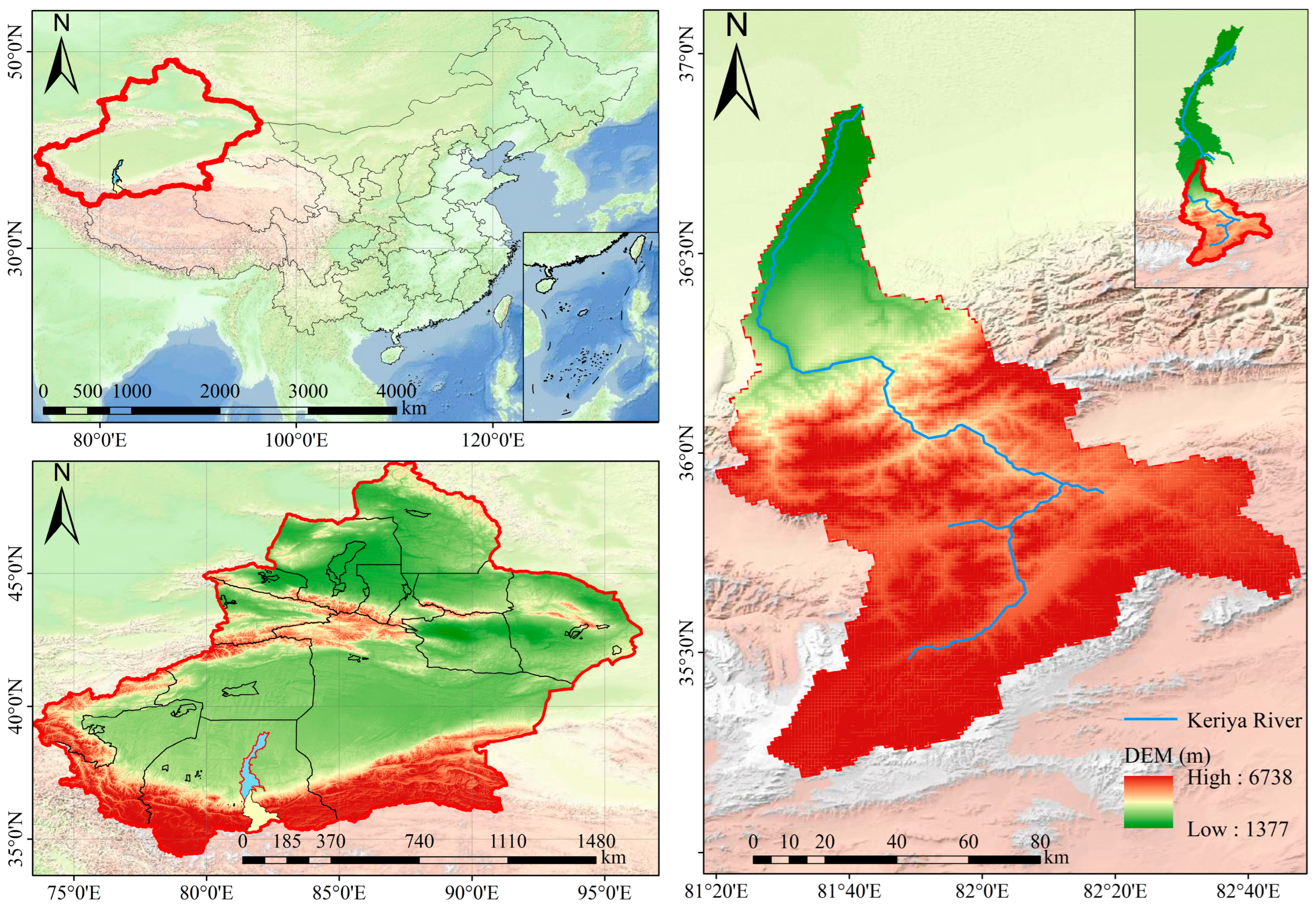
The Keriya River originates on the northerly slope of Mount Ustenger at the mid-section of the Kunlun Mountains, situated at the southernmost tip of Xinjiang. The geographical coordinates of its headwaters (35°50′~36°40′ N, 81°15′~82°30′ E) are shown in Figure 1. This region is a crucial glacial recharge area on the southern edge of the Tarim Basin. The topography of the study region is intricate, with altitudes ranging from 1377 to 6738 m, presenting a gradient that is higher in the south and lower in the north. The average elevation exceeds 5000 m, with the highest peak, Qong Muztag Peak, reaching 6962 m [18]. According to the Second Glacier Inventory, a total of 387 modern glaciers have developed in this region, covering a total area of 689 km [19]. The annual temperature range in the study area is approximately −17.6 to 7.9 °C, generally exhibiting a distribution pattern of colder conditions in the south and warmer conditions in the north. Precipitation distribution within the study area is uneven across the seasons, with annual average precipitation ranging from approximately 1.08 to 168.2 mm. Seasonal characteristics are marked by a long winter with extremely low temperatures and a short summer with relatively mild temperatures. The snow season is relatively long throughout the year, with most of the area covered by snow and ice; variations in this have a significant impact on the development of local agriculture and animal husbandry and are one of the decisive factors in the economic development of the local area and its downstream river basins.

2.2. Data Sources

2.2.1. Remote Sensing Data

The Landsat 7 and Landsat 8 remote sensing datasets used in this study were provided by the Earth Resources Observation and Science (EROS) Centre of the United States Geological Survey (USGS) (https://earthexplorer.usgs.gov/, accessed on 21 January 2025). The time resolution of these datasets is 16 days, the spatial resolution is 30 metres, and they comprise 11 bands; the data is projected using the Universal Transverse Mercator (UTM) projection [20]. Taking into account the issue of missing strips caused by the failure of the Landsat 7 on-board Scanning Line Corrector (SLC) in 2003 [21], this study selected Landsat 7 ETM+ Level-1 products (Path 149/Row 34) from 2005 to 2013 and Landsat 8 OLI/TIRS Level-1 data (Path 149/Row 34) from 2013 to 2024. The aforementioned datasets (see Table 1) collectively cover 436 scenes of imagery from the headwaters of the Keriya River.

2.2.2. Meteorological Data

The climatological data are sourced from the 1-kilometre resolved dataset of monthly mean temperatures and monthly precipitation in China for the period 1901–2024, provided by the National Earth System Science Data Centre (http://www.geodata.cn); data from 2005 to 2024 were selected (Table 1). This dataset was generated through spatial downscaling of CRU’s global 0.5° climate data and World Clim’s global high-resolution climate data using the Delta spatial downscaling scheme for the Chinese region. It was validated using data from 496 independent meteorological observation stations, and the validation results are reliable. It is currently the monthly climate dataset in China with the longest time series, highest spatial resolution and widest coverage [22,23].
To achieve pixel-level alignment with 30 m resolution Landsat imagery, this study resampled the 1 km meteorological data to 30 m using bilinear interpolation. It should be emphasised that resampling does not increase the spatial information content of the original data, but it enables spatial alignment of multi-source data, facilitating correlation analyses between snow/ice cover and meteorological variables at the pixel scale. Resampling may introduce local spatial artefacts in areas of high elevation and rugged terrain; however, overall trends and correlations remain consistent. It is primarily used for data integration and pixel-level matching and has a limited impact on the macro-scale analysis of climate signals.

2.2.3. DEM Data

The Digital Elevation Model (DEM) data was sourced from the Geospatial Data Cloud (http://www.gscloud.cn/); this data is based on SRTM version 4.1 (Table 1) and has a spatial resolution of 90 m. In this study, bilinear interpolation was used to resample the DEM data to 30 m resolution for the delineation of elevation zones and the analysis of the spatial distribution of snow and ice. It should be noted that whilst resampling the DEM improves the accuracy of spatial resolution, it does not increase the amount of original topographic information; consequently, it may introduce spurious accuracy or local spatial artefacts in pixel-level analyses. This phenomenon varies to some extent in areas of steep slopes; however, for the overall analysis of the spatial coupling between snow/ice and climatic variables, the resampling process is considered to be of acceptable reliability [24].

2.3. Data Processing

2.3.1. Cloud Removal

As the study area is situated in high-altitude mountainous terrain, the original Landsat imagery is severely affected by persistent cloud cover; the issue of cloud contamination in long-term snow/ice mapping cannot be overlooked [25]. This study employs the Fmask (Function of Mask) algorithm to perform automated detection and masking of clouds and cloud shadows for each image. A cloud mask layer is generated by analysing spectral and spatial texture features of the imagery. Given the difficulty in distinguishing snow from clouds under high-reflectance conditions, the new Fmask 4.0 algorithm introduces the spectral-contextual snow/ice index (SCSI), which significantly improves the accuracy of cloud–snow discrimination in polar and high-altitude settings [26], and can effectively support the snow/ice cover extraction in this study. Upon completion of the cloud masking process, all pixels identified as clouds or cloud shadows are uniformly marked and removed and are excluded from subsequent calculations of the Normalised Difference Snow Index (NDSI) and snow cover statistics.

2.3.2. Calculation of Snow/Ice Cover

To analyse the temporal variation in snow/ice cover within the study area, this study systematically processed Landsat imagery from 2005 to 2024. First, the original digital number (DN) values were converted to surface reflectance through radiometric calibration and the Quick Atmospheric Correction method to eliminate the influence of aerosols. On this basis, the Normalised Difference Snow Index (NDSI) was calculated using the green band (Landsat 7 Band 2/Landsat 8 Band 3) and the shortwave infrared band (Landsat 7 Band 5/Landsat 8 Band 6). This index effectively identifies the presence of snow and ice cover on the surface, including seasonal snow and glacial ice, as it is sensitive to the characteristic high reflectance of snow and ice in the visible green band and low reflectance in the shortwave infrared band. The formula is as follows:
N D S I = G r e e n S W I R G r e e n + S W I R
In Equation (1), G r e e n represents the green band, and S W I R represents the short-wave infrared band.
Based on existing research, this study adopts 0.3–0.5 as empirical thresholds [27,28,29] to extract candidate snow/ice-covered areas. A secondary spatial clipping is then performed by combining the NDSI mask with the study area’s vector boundaries, and the Band Math tool (logical expression: b 1 × b 1 b 1 ) is used to remove invalid edge pixels, thereby precisely delineating the snow/ice-covered area. Finally, the snow/ice-covered area is calculated based on pixel statistics at a 30-metre resolution.

2.3.3. Zoning of Snow/Ice Cover

This study first projected the 30-metre resolution snow/ice cover binary imagery generated by ENVI V5.6 and the SRTM DEM data into the WGS_1984_UTM_Zone_44N coordinate system (EPSG:32644) and then extracted the data using a mask based on the study area boundaries. Subsequently, the DEM was divided into six elevation bands (≤2000 m, 2000~3000 m, 3000~4000 m, 4000~5000 m, 5000~6000 m and ≥6000 m), and discrete elevation classes were generated through reclassification. Finally, using a bin-wise statistical method, the number of snow/ice-covered pixels within each elevation band was calculated. The snow/ice-covered area corresponding to each elevation interval was determined by dividing the product of the image pixel count and the resolution by the total area of that elevation interval (Table 2), thereby yielding the proportion of snow/ice-covered area for each elevation interval.

2.3.4. Meteorological Data Processing

In this study, multidimensional tools were employed to reconstruct the raw NetCDF-formatted data into raster datasets along the temporal dimension; following temporal filtering, these were exported in GeoTIFF format. Subsequently, a projection was defined to unify the coordinate system to GCS_WGS_1984, and spatial clipping was performed using the study area’s boundary vector data. Finally, based on the clipping results, the arithmetic mean of each pixel was extracted to serve as the spatial mean of the climatic elements for that month.

3. Research Methods

3.1. Snow/Ice Cover Indicators

Snow/Ice Cover Percentage (SICP) is used to characterise the relative area of snow and ice; it refers to the ratio of the area covered by snow and ice within a single pixel to the total area of that pixel [30] and is used to accurately characterise the extent of snow and ice cover within a region. The calculation formula is as follows:
S I C P = P S n o w / I c e P × 100 %
In Equation (2): P S n o w / I c e represents the snow/ice-covered area within the study area; P represents the total area of the region.

3.2. Trend Analysis

This study employs a simple linear regression analysis to examine the temporal and spatial trends in snow/ice cover in the headwaters of the Keriya River from 2005 to 2024. The trend slope from the multi-year regression equation is used as the rate of change for interannual or intra-annual analysis [31], and the calculation formula is as follows:
S l o p e = i = 1 n x i x ¯ × S I C P i S I C P ¯ i = 1 n x i x ¯ 2
In Equation (3), S l o p e is the slope of the regression equation, representing the trend and rate of change of snow/ice cover ( S I C P ) over time ( x ). When S l o p e > 0 , this indicates that S I C P shows an upward trend during the period n ; when S l o p e < 0 , this indicates a downward trend; when S l o p e = 0 , this indicates no significant trend; x i is the time-independent variable, representing the i  th year(or the i  th month of a given year); x ¯ is the arithmetic mean of all time points x i within the study period; S I C P i is the observed snow/ice cover value corresponding to time x i ; S I C P ¯ is the arithmetic mean of all S I C P i within the study period; n is the length of the study period, i.e., the total number of time units included in the trend analysis (e.g., total number of years, total number of months).

3.3. Correlation Analysis

This study employs Pearson’s correlation analysis to investigate the relationship between snow/ice cover, temperature and precipitation, in order to explore the links between the three variables [32], using the following formula:
R x y = i = 1 n x i x ¯ y i y ¯ i = 0 n x i x ¯ i = 0 n y i y ¯
In Equation (4), n represents the cumulative number of years in the statistical period, x i and y i are the two variables under analysis. x ¯   and   y ¯ are the annual averages of the two variables n , respectively. When 1 > R x y > 0 , a positive correlation is indicated; when 1 < R x y < 0 , a negative correlation is indicated. The closer the absolute value of R x y is to 1, the higher the correlation between the two variables.

3.4. Construction of the Prediction Model

This study constructs an optimal fitting prediction system based on multi-model fusion to characterise the future changes in snow/ice cover, precipitation and air temperature in the headwaters of the Keriya River from 2025 to 2044. By comparing multiple algorithms, the system selects the most suitable model and combines trend factors, seasonal fluctuations and stochastic variability to generate physically meaningful prediction results. The specific process comprises four parts: data pre-processing, multi-model training and validation, selection of the optimal model, and future scenario forecasting.

3.4.1. Data Pre-Processing

A time-series dataset was constructed using monthly snow/ice cover (%), precipitation (mm) and air temperature (°C) data from the headwaters of the Keriya River for the period 2005–2024. First, the raw data were standardised in the temporal dimension to generate time indices and annual/monthly identifiers. Periodic, lagged and rolling statistical features were then constructed to capture temporal patterns. The core calculation formulas are as follows:
Sin m o n t h = sin 2 π × m o n t h 12
Cos m o n t h = cos 2 π × m o n t h 12
R o l l i n g m e a n k = 1 k i = t k + 1 t X i
In Equations (5)–(7): m o n t h denotes the month (1–12); k denotes the sliding window length (3, 6, 12); X i denotes the snow/ice cover/precipitation/temperature value for the i period; R o l l i n g m e a n k denotes the moving average over a length of k . After imputing all missing values in the features with the mean, standardisation was performed using S t a n d a r d S c a l e r to eliminate differences in units.

3.4.2. Multi-Model Training and Validation Framework

The data from 2005 to 2019 was designated as the training set (180 months in total), whilst the data from 2020 to 2024 was designated as the test set (60 months in total). Six types of regression prediction models were constructed to form a comparative framework:
  • Linear Regression Model
The least squares method is used to fit a linear relationship, with the model form as follows:
Y = β 0 + β 1 X 1 + β 2 X 2 + + β n X n + ϵ
2.
Random Forest Regression
Random forest regression is a decision tree model based on ensemble learning that constructs multiple decision trees and aggregates the results. The parameters are set as follows: number of trees ( n estimators ) = 200, maximum depth ( max d e p t h ) = 12, minimum split sample size ( m i n _ s a m p l e s _ s p l i t = 5 ) and minimum leaf node sample size ( m i n _ s a m p l e s _ l e a f = 2 ).
3.
Gradient Boosting Regression
This employs a sequential ensemble method to reduce residuals through iterative optimisation. The parameters are set as follows: learning rate l e a r n i n g r a t e = 0.05 , number of iterations n estimators = 150 , maximum depth max depth = 6 and minimum split sample size min samples _ split = 5 .
4.
Support Vector Regression (SVR)
Support vector regression is a high-dimensional mapping method based on kernel functions, utilising the radial basis function (RBF) kernel:
K ( x i , x j ) = exp ( γ | x i x j | 2 ) , regularisation parameter C = 100 , kernel coefficient γ = 0.1 .
5.
Multi-Layer Perceptron (MLP)
Construct a feedforward neural network comprising two hidden layers (with 100 and 50 neurons, respectively), using the activation function ReLU :   f ( x ) = max ( 0 , x ) and the Adam optimiser.
6.
Autoregressive Integrated Moving Average (ARIMA) Model
Specifically designed for time-series forecasting, the model is of the form  A R I M A ( p , d , q ) , where:
Snow/ice cover: ARIMA ( 2 , 1 , 1 ) × ( 1 , 1 , 1 ) 12 ;
Precipitation: ARIMA ( 1 , 1 , 2 ) × ( 1 , 1 , 1 ) 12 ;
Air temperature: ARIMA ( 2 , 1 , 2 ) × ( 1 , 1 , 1 ) 12 .
Model performance is quantified using the Mean Absolute Error ( M A E ), the Root Mean Square Error ( R M S E ) and the coefficient of determination ( R 2 ) [33], calculated as follows:
M A E = 1 n i = 1 n y i y ^ i
R M S E = 1 n i = 1 n y i y ^ i 2
R 2 = 1 i = 1 n ( y i y ^ i ) 2 i = 1 n ( y i y ¯ ) 2
In Equations (8)–(10): n represents the number of samples in the test set; y i denotes the observed value for period  i ; y ^ i denotes the model’s predicted value for period i ; and y ¯ denotes the mean of the observed values. The smaller the values of M A E and R M S E , and the closer R 2 is to 1, the better the model’s fitting performance.

3.4.3. Selection of the Optimal Model

Select the optimal fitting model for each variable using the coefficient of determination ( R 2 ) as the core metric [34]: sort all models in descending order by R 2 and select the model corresponding to the maximum value of R 2 as the baseline prediction model for that variable; in the extreme case where R 2 is negative, the random forest model is selected by default as a fallback solution to ensure the stability of the prediction system.

3.4.4. Future Scenario Forecasting

Based on the baseline forecast values output by the optimal model, a monthly forecast model for 2025–2044 is constructed by integrating trend factors, seasonal adjustments, random fluctuations and cyclical climate variations. The specific technical approach is as follows:
Generation of baseline forecasts
The selected optimal model (random forest, ARIMA, etc.) is used to perform full-sample training on the training set (2005–2024), generating monthly baseline forecast values for 2025–2044 y model , t .
Quantification of trend factors
Based on historical data (2005–2024), the Mann–Kendall trend test and Sen’s slope estimation method were employed to quantify the interannual trends of each variable [35]:
α s n o w / i c e = m e d i a n y j y i j i i < j
α p r e c i p = 1 n 1 t = 2 n ( Y t Y t 1 )
α t e m p = t = 1 n ( t t ¯ ) ( T t T ¯ ) t = 1 n ( t t ¯ ) 2
In Equations (11)–(13): α s n o w / i c e , α precip and α temp represent the interannual trend factors for snow/ice cover, precipitation and air temperature (%/year, mm/year, °C/year), respectively; y i and y j denote the annual mean snow/ice cover for the years i and j , respectively; Y t denotes the total annual precipitation for the year t ; T t denotes the annual mean air temperature for the year t ; and n = 20 denotes the number of forecast years.
Determination of weight optimisation
The Bayesian Model Averaging (BMA) framework is employed to determine the optimal weights between model predictions and historical climate data [36]:
ω = R model 2 R model 2 + R climatology 2
In Equation (14), R model 2 is the coefficient of determination of the optimal model on the independent validation set (2015–2019); R climatology 2 is the coefficient of determination of the historical monthly mean sequence over the same period (in the integrated forecast model, this can be calculated from Equation (14) to yield ω snow / ice = 0.8 , ω precip = 0.7 and ω temp = 0.75 ).
Climate cycle identification
Identification of significant cycles in historical data based on Singular Spectral Analysis (SSA) and Fourier transforms [37]:
P ( f ) = t = 1 n X t e i 2 π f t 2
In Equation (15): X t denotes the time-series value after trend removal for period t ( t = 1 , 2 , , n ); and f  denotes the frequency, f = k n , where k = 0 , 1 , , n 1 .
Modelling stochastic fluctuations
The residual series is modelled using an autoregressive conditional heteroscedasticity (ARCH) model to capture the clustering of fluctuations:
ε t = σ t z t
z t ~ N ( 0 , 1 ) σ t 2 = α 0 + i = 1 q α i ε t i 2
In Equations (16) and (17), ε t represents the residuals after trend and stationarity removal; σ t 2 represents the conditional variance; and q = 1 represents the ARCH order.
Probabilistic modelling of extreme events
Fitting precipitation extremes using the Generalised Pareto Distribution (GPD) [38]:
F ( x ) = 1 1 + ξ x u σ 1 / ξ , x > u
In Equation (18), u is the threshold (taken as the 95th percentile from historical data); σ is the scale parameter; ξ is the shape parameter. The frequency of historical extreme precipitation ( x > u ) is 7.6%; based on this, the probability of future extreme events is set at 8%.
Integrated prediction model
The final forecast value is calculated using the following equation:
Y t = ω y model , t + ( 1 ω ) μ m + α Δ t + k = 1 K γ k sin 2 π t τ k + ϕ k + ε t + I t E t
In Equation (19): Y t : the final forecast value for the t  th period; y model , t : the baseline forecast value of the optimal model; μ m : the historical monthly mean ( m = 1 , , 12 ); Δ t : the time difference (in years) from the base year (2024); γ k τ k ϕ k : the amplitude, period and phase of the k  th climate cycle; ε t : the random fluctuation term (following an ARCH process); I t : the extreme event indicator variable (Bernoulli distribution, p = 0.08 ); E t : the intensity of extreme events (GPD distribution).

4. Results

4.1. Temporal Variations in Snow/Ice Cover

4.1.1. Characteristics of Intra-Annual Variations in Snow/Ice Cover

By using the average snow/ice cover percentage (SCIP) for each month from 2005 to 2024 as the SCIP for that month, a 12-month time series of snow/ice cover percentage was obtained. At the same time, the averages for March to May, June to August, September to November and December to February correspond to the SCIP seasonality sequences for spring, summer, autumn and winter, respectively. An analysis of the intra-annual variations in the SCIP of the headwaters of the Keriya River was conducted at both monthly and quarterly scales.
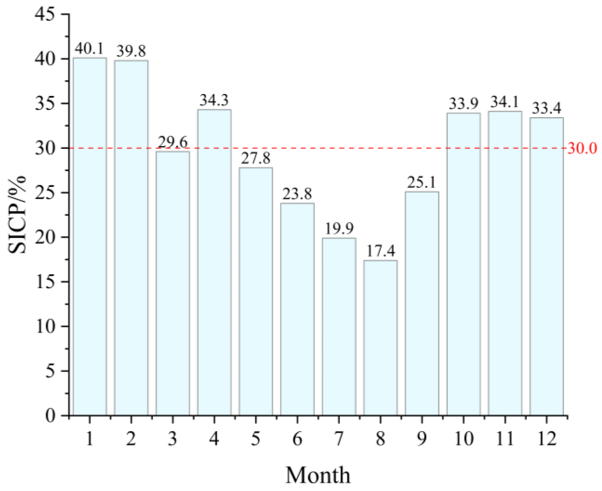
Based on the monthly mean snow/ice cover values from 2005 to 2024, a map of the monthly average snow/ice distribution in the headwaters of the Keriya River was produced (Figure 2). Inter-monthly variations show that snow/ice cover is highest in January, at 40.1%; it decreases slightly to 39.78% in February, remaining at a high level. In March, it dropped significantly to 29.6%, marking the onset of the rapid melting period; in April, it rebounded to 34.3%, before falling again to 27.8% in May. It continued to decline from June to August, reaching 23.8%, 19.9% and 17.4%, respectively, with August recording the lowest figure of the year. In September, snow/ice cover rebounded to 25.1%, marking a turning point in the downward trend; it rose to 33.9% in October and continued to rise to 34.0% in November, approaching winter levels. In December, it fell slightly to 33.4%, yet remained at a relatively high level. The multi-year average snow/ice cover during the study period was 30.0%, exhibiting a ‘single-peak’ distribution, with the peak occurring in January and the trough in August, a difference of 22.62 percentage points, reflecting the sensitivity of snow/ice cover to climatic fluctuations throughout the year.
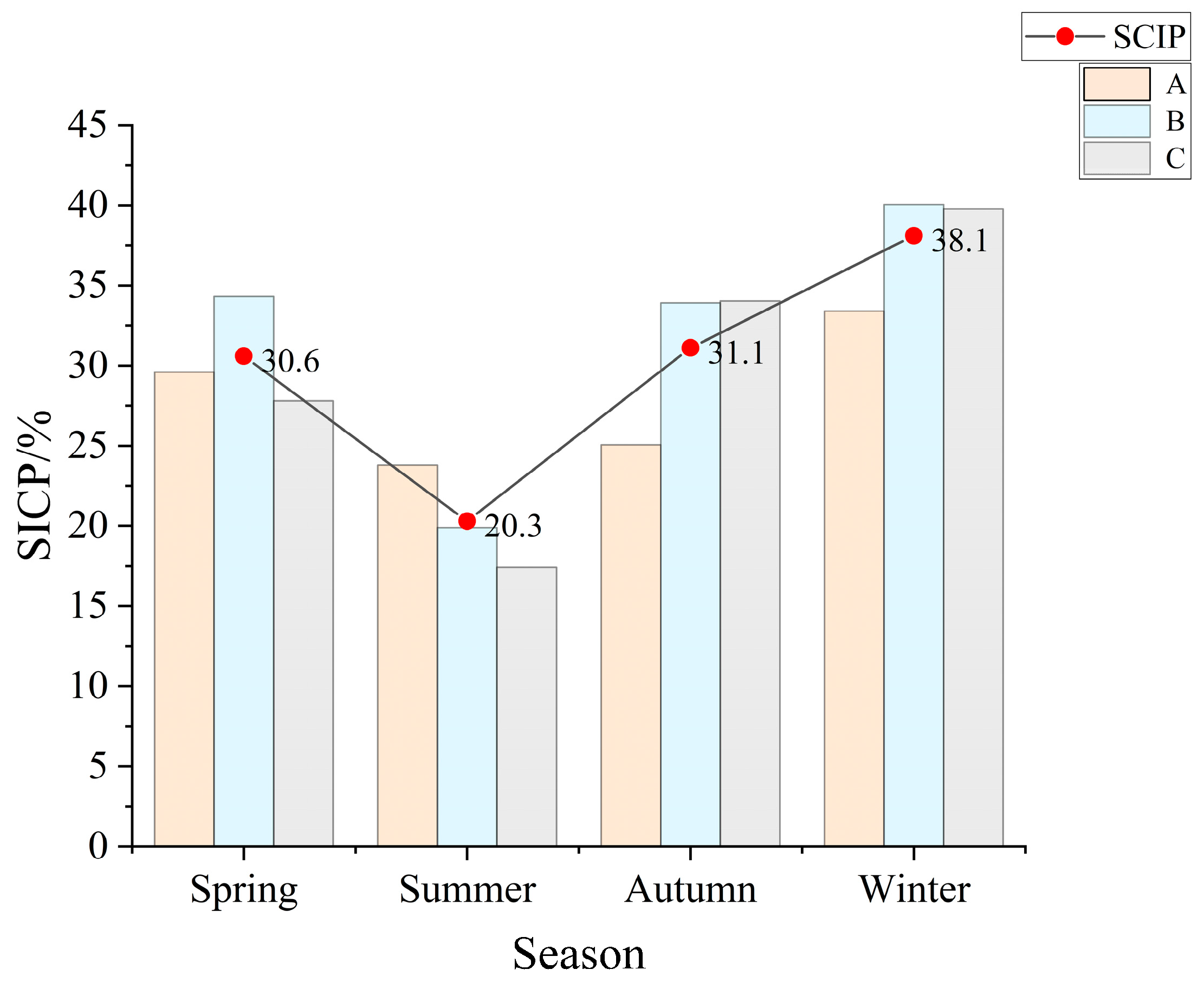
To reveal the seasonal evolution of snow/ice cover in the headwaters of the Keriya River, based on monthly snow/ice cover data from 2005 to 2024, as shown in Table 3, the average snow/ice cover percentage (SCIP) for the four seasons—spring, summer, autumn and winter—was calculated for three different monthly combinations: March, June, September and December (Group A); April, July, October and January(Group B), and May, August, November, and February (Group C), to calculate the average snow/ice cover percentage (SCIP) for spring, summer, autumn and winter, respectively, thereby identifying the differing contributions of various months to seasonal snow/ice characteristics (Figure 3).
On a seasonal average, SCIP is lowest in summer (20.3%), followed by autumn (31.0%) and spring (30.6%), with winter recording the highest figure (38.1%). Overall, this exhibits a single-peaked annual variation pattern characterised by ‘high in winter, low in summer, and transitional in spring and autumn’. Further analysis of SCIP variations across different monthly combinations within each season reveals that in spring (March—May), Group B (April) had the highest SCIP (34.3%), followed by Group A (March) (29.6%), with Group C (May) recording the lowest (27.8%). In April, snow/ice cover remained relatively high; however, SCIP declined markedly in May, with the low value in Group C for May dragging down the overall level. Summer (June—August): SCIP showed a continuous downward trend across all three groups, with Group A (June) recording the highest value (23.8%), followed by Group B (July) (19.9%), and Group C (August) recording the lowest (17.4%). August marked the annual trough for SCIP (average 11.6%), with high-temperature-driven melting reaching its peak at this time; the extremely low August value in Group C dragged down the summer average. Autumn (September—November): SCIP in Group B (October) and Group C (November) were similar (33.9% and 34.0%), significantly higher than in Group A (September, 25.1%). This reflects the slow accumulation of snow/ice in September; however, from October onwards, precipitation predominantly took the form of snowfall, leading to rapid snow/ice accumulation; this trend continued into November, with snow/ice cover continuing to increase. Winter (December—February): Groups B (January) and C (February) recorded the highest SCIP values (40.0% and 39.8%), with Group A (December) slightly lower (33.4%). January marked the annual peak for SCIP (average 63.2%); although there was a slight decline in February, levels remained high. December, being the early winter period, saw snow/ice cover still accumulating and had not yet reached a stable high-value state.

4.1.2. Characteristics of Interannual Variations in Snow/Ice Cover

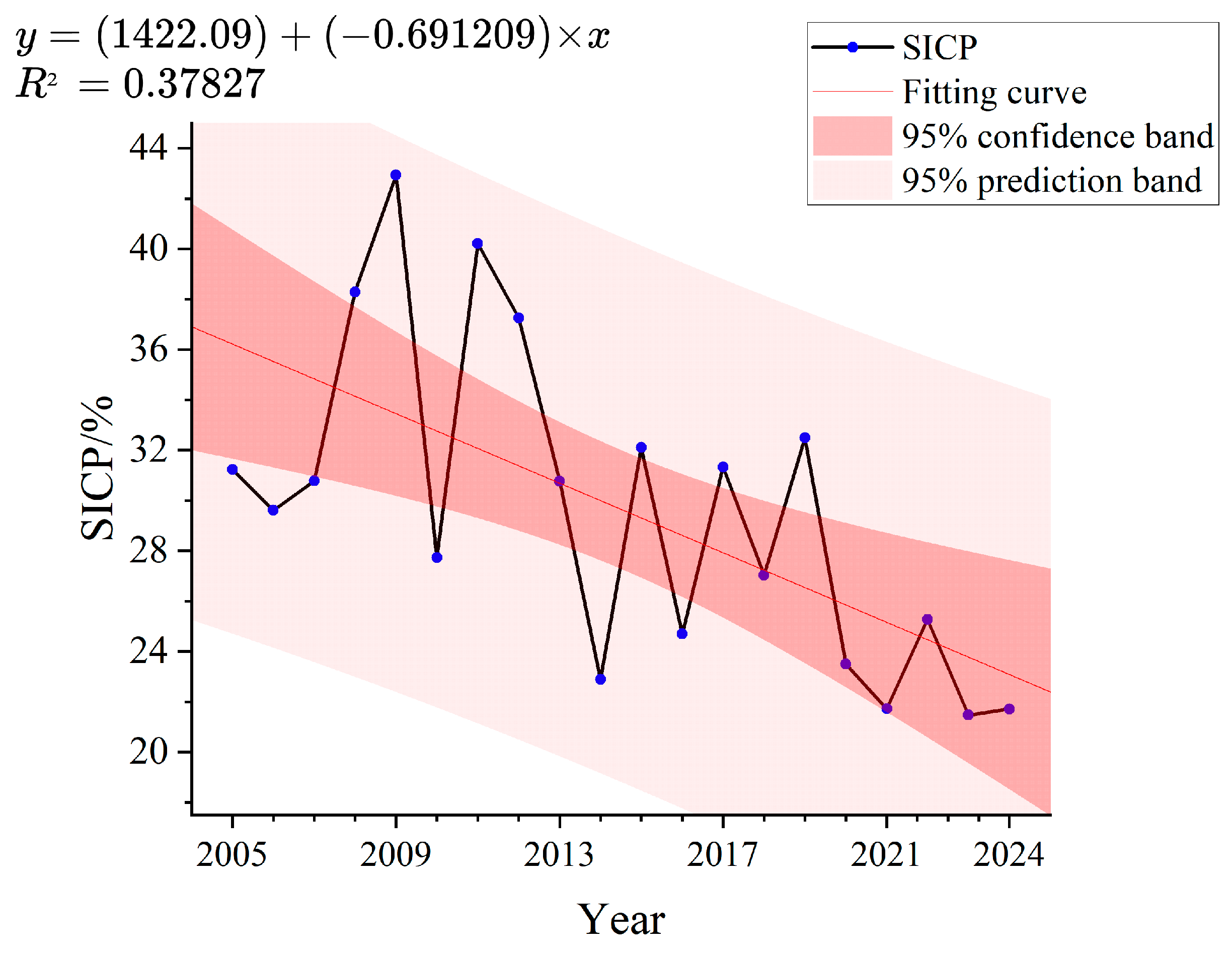
Based on SCIP calculations for the Keriya River from 2005 to 2024, the interannual variation in snow/ice cover can be determined using the annual average SCIP value as the representative value for that year (Figure 4).
Overall, SCIP in the headwaters of the Keriya River shows a non-significant decreasing trend, declining at an annual rate of −0.69%. The interannual variations in snow/ice cover within the study area exhibit phased trends of increase or decrease. Specifically, the average SCIP for the period 2006–2009 showed an upward trend, rising by 3.32% annually, with SCIP reaching its highest value in nearly 20 years in 2009, at 43.0%. The average SCIP for 2011–2014 showed a marked downward trend, decreasing by 17.31% annually. The average SCIP for 2015–2024 exhibited a fluctuating downward trend, decreasing by 1.03% annually, and reached the lowest SCIP value in the past 20 years in 2023, at 21.5%.
The above classification is based on statistical trend breakpoints (such as around 2011) and significant extreme years (the peak in 2009 and the trough in 2023), objectively identifying the primary rhythms of interannual SCIP variation. These phasic fluctuations highlight the complexity of snow/icepack response to climate, yet the SCIP in the study area overall exhibits a continuous decreasing trend, which is closely linked to global warming [17,39].
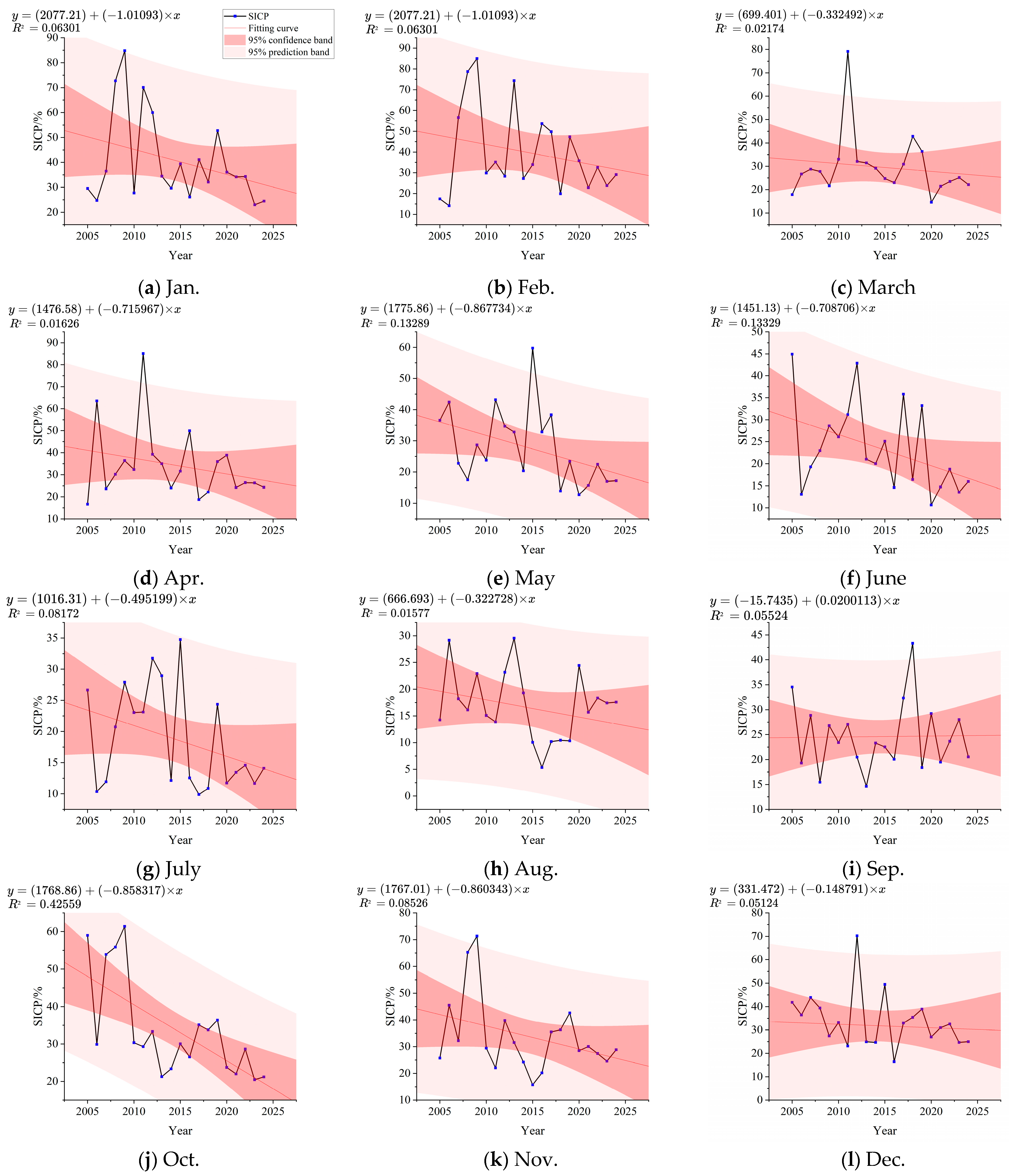
Analysing snow/ice cover percentage by month (Figure 5), both January and February showed a continuous decline at a rate of 1.01% per decade, with a significant downward trend; in March, apart from an abnormally high value in 2011, the SCIP was generally below 50.0%, with an average annual decline of 0.33% and a continuing slowdown; in April, the SCIP value rose slightly compared with March, but continued to decline annually at a rate of 0.71%; the changes in May were particularly pronounced, with the peak year shifting to around 2015 and the overall decline accelerating to a rate of 0.86%; in June, most values were below 45.0%, with some extremely low values observed, and the rate of decline was 0.70%; the distribution of data in July was polarised, with approximately half of the years concentrated between 25.0% and 35.0%, whilst the majority of the remainder were close to 10.0%; the average for August was the lowest of the year, generally below 30.0%, with an exceptionally low record in 2019, during which the value declined slowly at a rate of 0.32%; September was the only month to show an upward trend, with a growth rate of approximately 0.02% and a relatively concentrated distribution of values; from October onwards, the downward trend intensified once more, with a rate of decline reaching 0.85%. Following 2013, the figures began to rebound, with the lowest values consistently remaining above 20.0%; the rate of decline in November was comparable to that of October, whilst the range was significant, reaching approximately 58.0%; although December also exhibited a declining trend, fluctuations were minimal, with SCIP stabilising around 35.0% in most years, and the rate of decline was merely 0.14%.
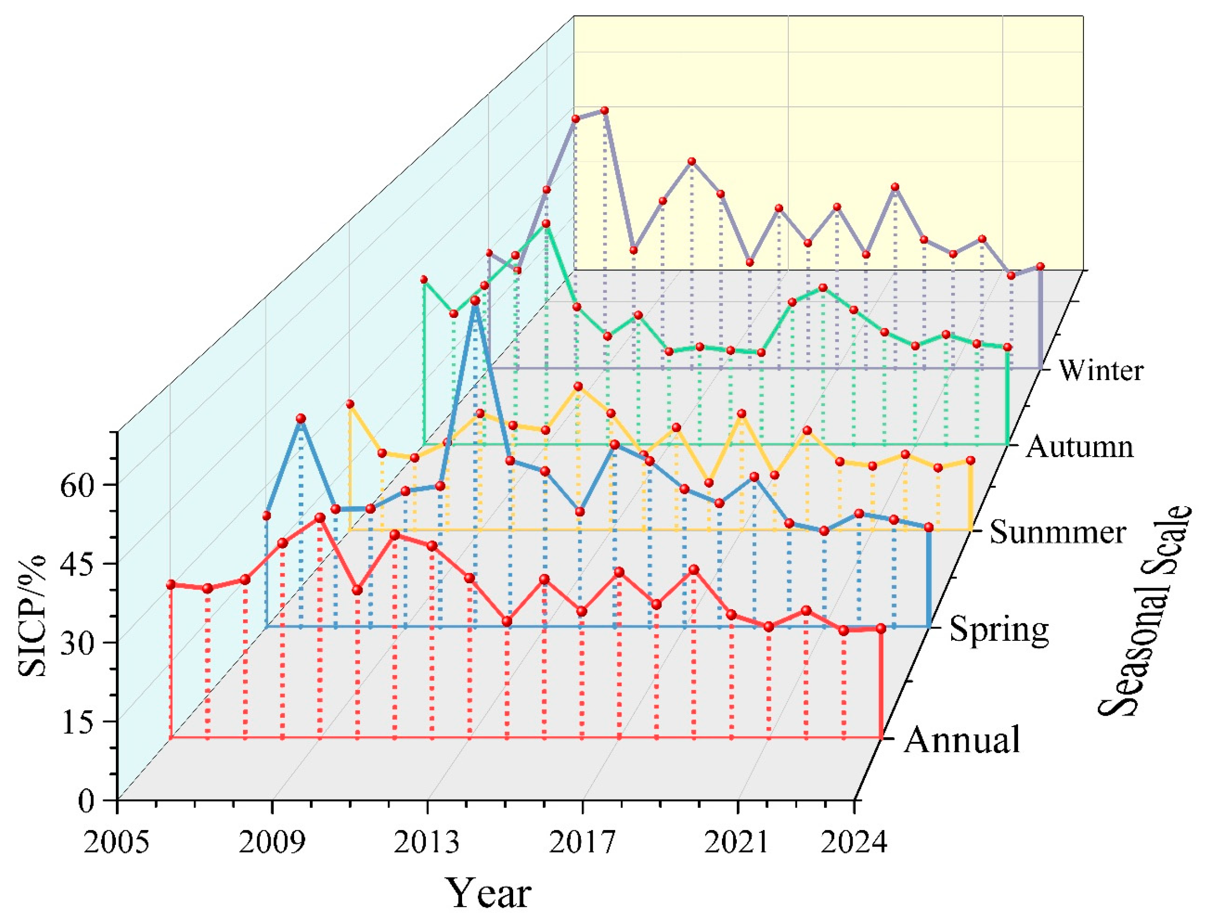
Based on seasonal average snow/ice cover data from 2005 to 2024, A map was produced showing the interannual variations in snow and ice cover across the spring, summer, autumn and winter seasons in the headwaters of the Keriya River (Figure 6). Overall, SCIP showed a fluctuating downward trend across all seasons, but there were significant differences in the amplitude of interannual fluctuations and the characteristics of different phases.
In spring (March to May), the interannual variation in SCIP ranges from 20.5% to 69.2%, with a range of 48.7 percentage points, making it the season with the most pronounced fluctuations among the four seasons. An unusually high value was recorded in 2011 (69.2%), while 2014, 2021 and 2023 were years with low spring values (24.5%, 20.5% and 22.8% respectively). In summer (June—August), the SCIP generally remains at a low level, with an interannual variation range of 10.8% to 32.6% and a range of 21.8 percentage points. 2012 (32.6%) was a relatively high summer value, while 2016 (10.8%) was an extremely low value. In autumn (September—November), SCIP ranged from 22.5% to 53.2%, with a range of 30.7 percentage points. The period from 2008 to 2009 was a high-value period for autumn (45.5%, 53.2%), while 2013–2016 was a low-value period (22.0%—23.0%). In winter (December–February), the SCIP ranged from 23.8% to 65.8%, with a range of 42.0 percentage points; the amplitude of fluctuation was second only to that of spring. Peak values were recorded in 2008–2009 (63.6% and 65.8%), whilst 2014, 2023 and 2024 were years of low values (27.2%, 23.8% and 26.2%).
In terms of phased changes, the spring, autumn and winter seasons all reached their highest values within the study period between 2005 and 2009, coinciding with the year of the highest annual average SCIP (2009). From 2010 to 2014, the divergence in SCIP across the seasons intensified, with significant fluctuations in spring, whilst the summer, autumn and winter seasons first declined and then rose. The period from 2015 to 2024 was characterised by fluctuating declines, with seasonal SCIP generally lower than in the preceding period. In particular, SCIP for all four seasons—spring, summer, autumn and winter—was at low levels in 2023, consistent with the overall trend of the annual average SCIP reaching its lowest value (21.5%) that year.

4.2. Spatial Variations in Snow/Ice Cover

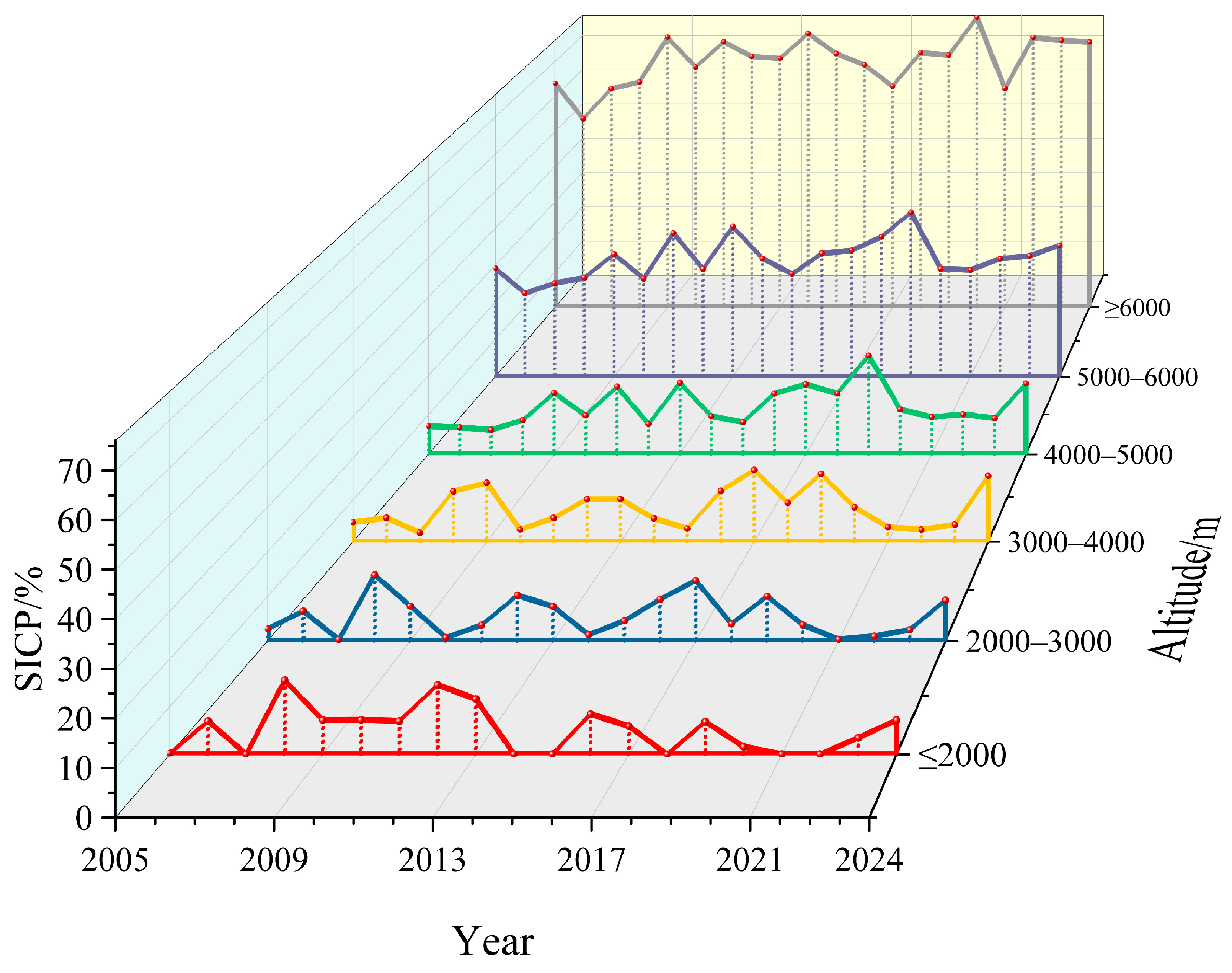
Among the factors influencing the spatiotemporal distribution of snow/ice cover, topography is one of the most significant factors [40]. Significant differences in temperature and precipitation at different altitudes result in marked variations in snow/ice cover distribution across different altitudinal zones. To investigate the relationship between snow/ice cover percentage (SCIP) and topographic factors in the headwaters of the Keriya River, the study area was divided into six altitude zones based on elevation, and the annual average SCIP for the 20 years from 2005 to 2024 was calculated for each zone (Figure 7). The results indicate that SCIP in this region is significantly positively correlated with elevation, with snow/ice cover percentage increasing gradually with rising elevation.
The SCIP was lowest in areas below 2000 m, with a 20-year average of 5.2%; the annual average SCIP in the 2000–3000 m and 3000–4000 m elevation zones was 5.7% and 8.3% respectively, with snow/ice cover remaining relatively low, representing the primary zones of unstable snow/ice distribution; In the 4000–5000 m elevation zone, the annual average SCIP rose to 12.4%, with a peak of 25.1% in 2019, indicating a marked increase in snow/ice cover; In the 5000–6000 m elevation range, the annual average SCIP increased significantly to 31.9%, with the most pronounced interannual fluctuations; the maximum value was recorded in 2019 (44.2%), with the minimum occurring in 2006 (22.5%); The annual average SCIP was highest in the region above 6000 m, reaching 70.3%, representing a zone of perennial stable snow/ice cover. The interannual variation in SCIP ranged from 53.7% to 82.5%, with overall values remaining consistently high.

4.3. Analysis of Meteorological Data

4.3.1. Characteristics of Temperature Variations in the Headwaters of the Keriya River

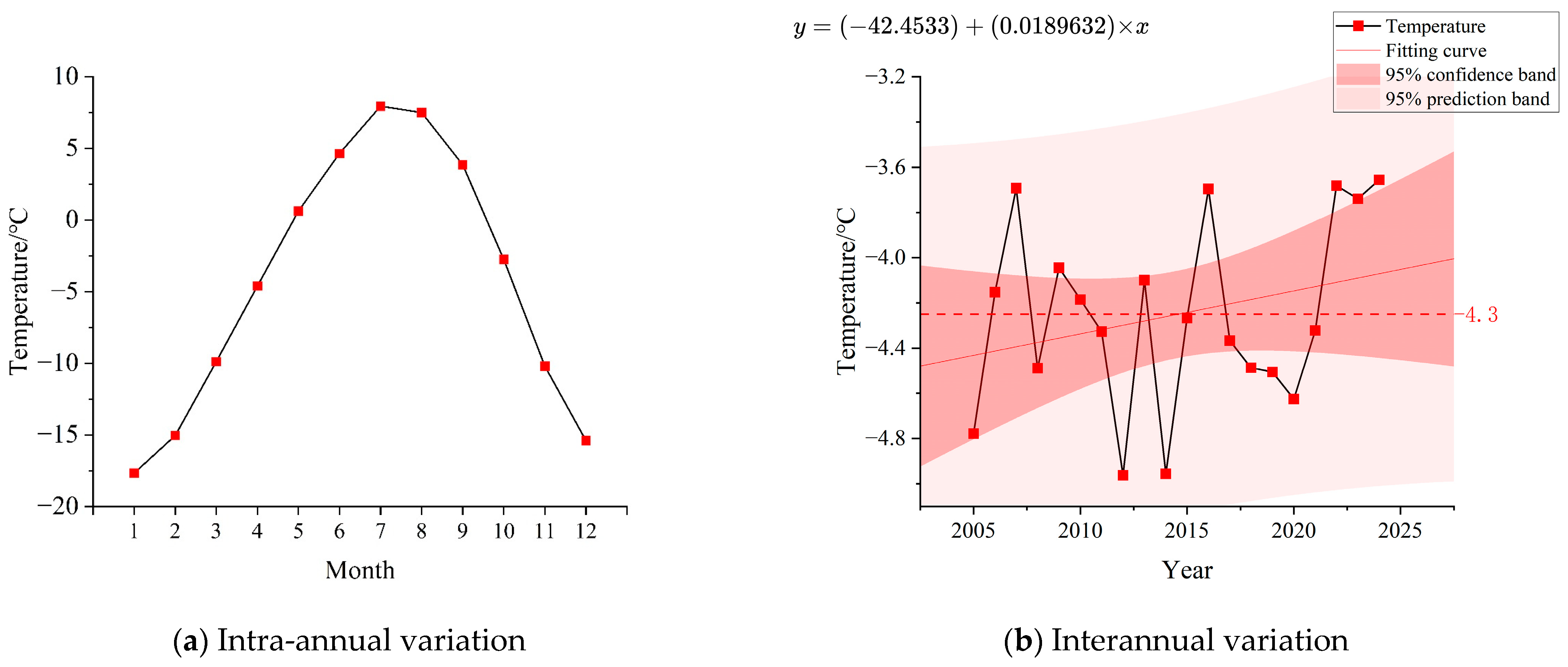
Temperatures in the headwaters of the Keriya River exhibit a significant warming trend and periodic fluctuations (Figure 8). Seasonal temperature variations are pronounced, with July being the warmest month (average 7.94 °C) and January the coldest (average −17.67 °C); the annual temperature range reaches 25.6 °C. Interannual variations show that between 2005 and 2024, the annual mean temperature in the study area was −4.25 °C, exhibiting an overall fluctuating upward trend with a linear warming rate of approximately 0.018 °C per year; during 2005–2010, the annual mean temperature was −4.23 °C, with a stable trend; from 2011 to 2015, temperatures decreased, with an annual average of −4.68 °C, of which 2012 was the coldest year (−4.96 °C); Temperatures rebounded slightly between 2016 and 2020, with an annual average of −4.54 °C; between 2021 and 2024, warming was pronounced, with the annual average temperature rising to −3.85 °C, and temperatures exceeding −3.75 °C for three consecutive years from 2022 to 2024. Over the past five years, the rate of warming has intensified, indicating that the trend towards climate warming in the region has been particularly pronounced in recent years.

4.3.2. Characteristics of Precipitation Changes in the Headwaters of the Keriya River

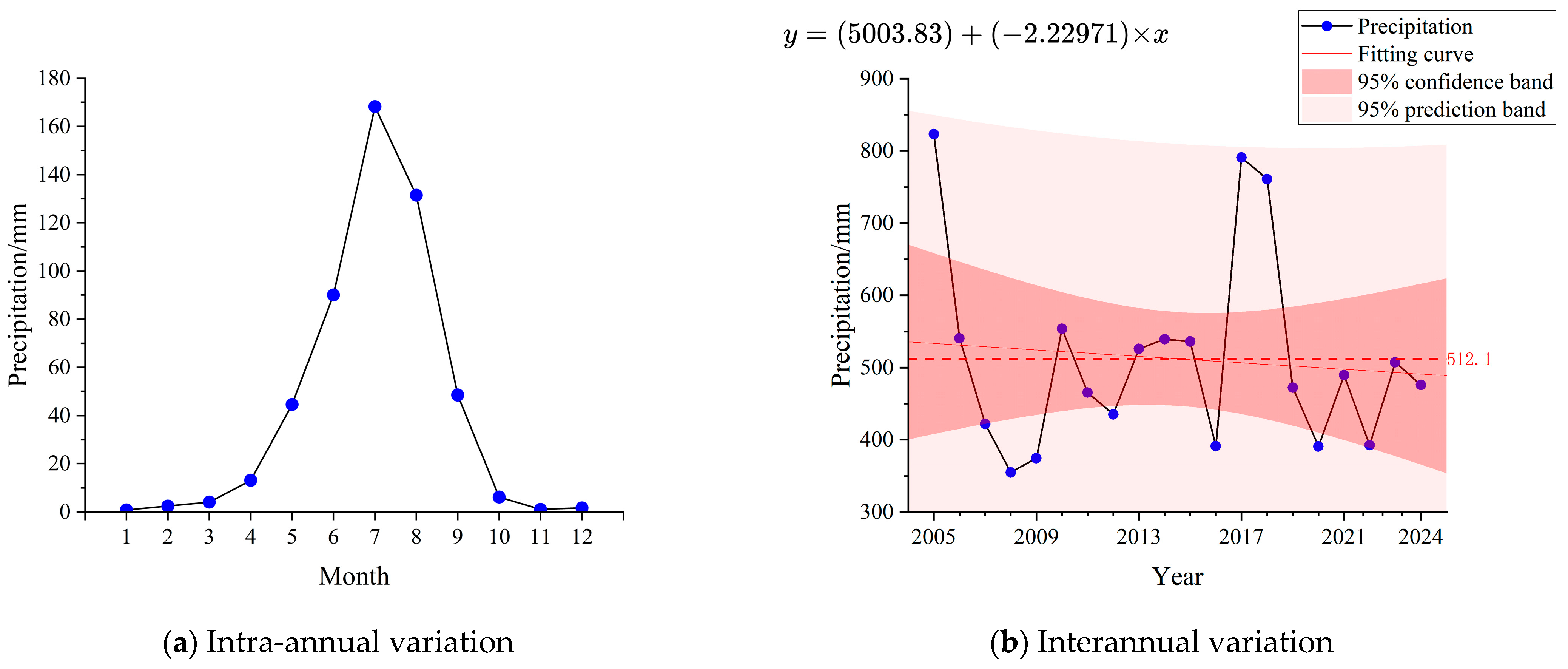
Precipitation in the headwaters of the Keriya River is distributed extremely unevenly across the seasons (Figure 9). The multi-year average precipitation in the study area for 2005–2024 was 512.1 mm, with severe interannual fluctuations (coefficient of variation Cv = 25.4%). Precipitation is distributed extremely unevenly throughout the year, with 68.2% of the annual total concentrated in the summer (June–August), of which July has the highest cumulative precipitation, reaching 167.4 mm, accounting for 32.7% of the annual total; whilst winter (December–February) accounts for only 2.1%. In terms of interannual variation, the period 2005–2009 was a relatively dry period, with a long-term average precipitation of 502.9 mm; the period 2010–2016 saw a slight increase, with a long-term average precipitation of 516.8 mm;2017–2018 saw exceptionally high rainfall, with a multi-year average precipitation of 775.9 mm; 2019–2024 saw a decline and a return to stability, with a multi-year average precipitation of 487.9 mm. Overall, precipitation exhibits significant seasonal concentration and interannual instability.

4.4. Relationship Between Snow/Ice Cover and Temperature and Precipitation

To investigate the temporal and spatial distribution features of meteorological data and snow/ice cover in the headwaters of the Keriya River, this study calculates the 20-year SCIP and the multi-year average correlation coefficients with temperature and precipitation, to explore in greater depth the correlation between snow/ice distribution and meteorological variables.
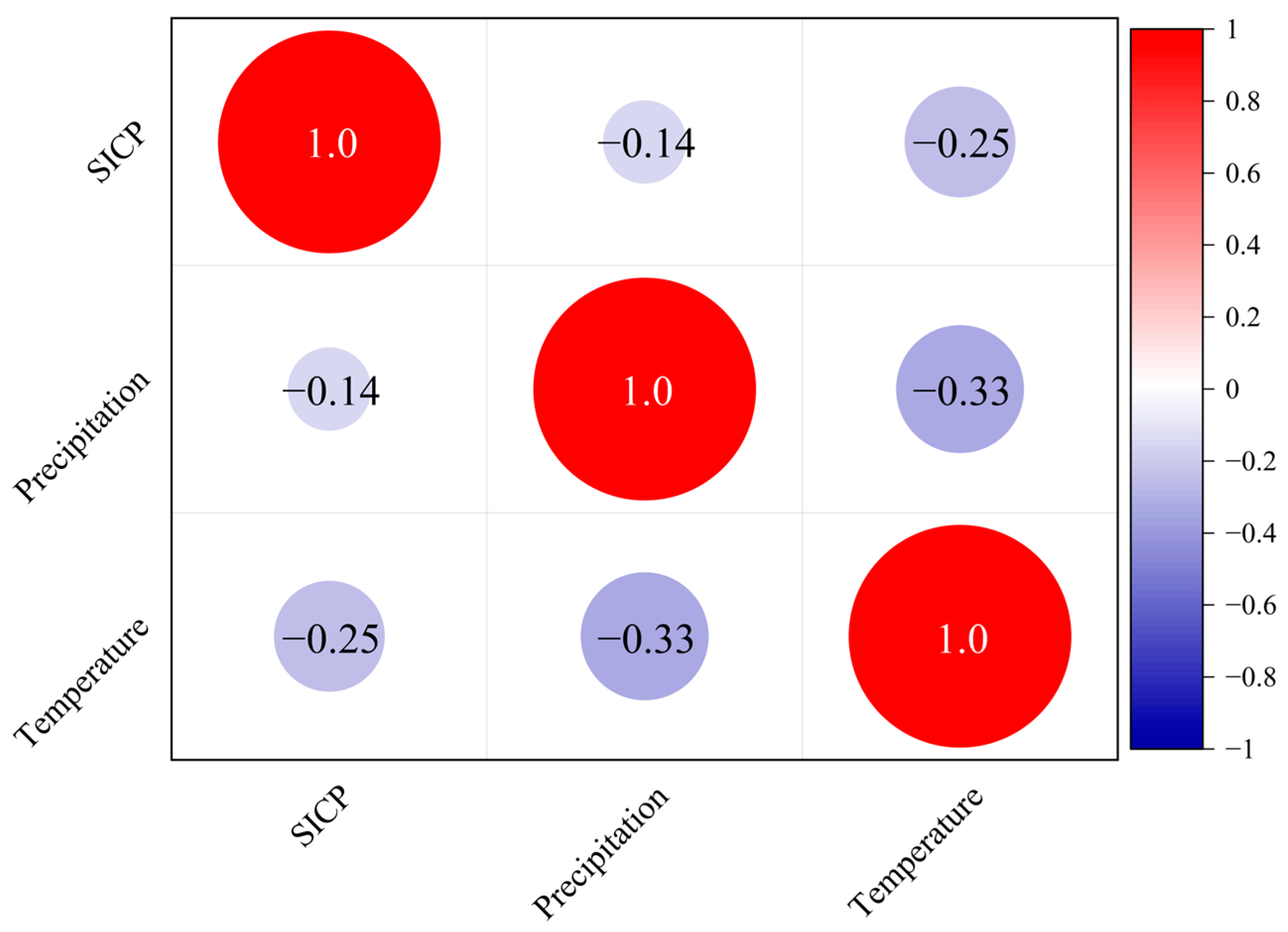
At the interannual scale (Figure 10), the correlation between snow/ice cover in the headwaters of the Keriya River and temperature and precipitation is relatively weak. The correlation coefficient between snow/ice cover and temperature is −0.25, indicating a slight negative correlation between the two, but this relationship is not significant. The correlation coefficient between snow/ice cover and precipitation is only −0.14, indicating an extremely weak correlation between the two.
To counteract the weakening of correlations caused by long-term averages and to uncover more precise correlations between variables, this study averaged the monthly SCIP and meteorological data over 20 years. The results of the analysis of the correlations between the variables every month are presented in the table below (Table 4).
On a monthly scale, the correlation between snow/ice cover and temperature and precipitation exhibits distinct patterns. In January, the correlation coefficient between snow/ice cover and temperature was 0.0034, whereas the correlation with precipitation was 0.34; low temperatures virtually halted the melting of snow and ice, and precipitation mainly replenished snow/ice cover in the form of snow. The situation in February was similar to that in January, with stable meteorological conditions; snow/ice cover was less affected by short-term fluctuations in temperature and precipitation. In March, temperatures began to rise slowly; the correlation coefficient between snow/ice cover and temperature was 0.02, whereas the correlation with precipitation was −0.31. This indicates that rising temperatures began to influence snow/ice melt, and precipitation gradually took the form of rain, exerting a negative effect on snow/ice cover. In April, temperatures rose further; the correlation coefficients between snow/ice coverage and temperature and precipitation were −0.13 and −0.44, respectively, with high temperatures and precipitation jointly accelerating the melting of snow and ice. From May to June, temperatures rose significantly; snow/ice coverage showed a negative correlation with temperature (−0.3), while increased precipitation, accompanied by more rainfall, further promoted melting. In July–August, the negative correlation reached its maximum (−0.35), with temperature becoming the dominant factor in snow/ice melt, while precipitation had a lesser influence. In September, temperatures dropped; the correlation coefficient between snow/ice cover and temperature was −0.5, whereas that for precipitation was 0.17. The drop in temperature slowed melting, and precipitation gradually replenished snow/ice in the form of snow. In October, the correlation coefficient between snow/ice cover and temperature was 0.45, and that for precipitation was 0.2; further, low temperatures and snowfall led to the recovery of snow/ice. In November, with lower temperatures, the correlation coefficients between snow/ice cover and temperature and precipitation were −0.17 and −0.37, respectively, and snow/ice cover remained relatively stable. In December, the cold environment and low precipitation levels caused snow/ice cover to enter a relatively stable state, with short-term meteorological fluctuations having a minor impact.
In summary, the simple linear relationship between SCIP and temperature and precipitation is generally weak, but the relationship among the three exhibits strong seasonal dependence and non-linear characteristics: temperature primarily exerts a negative, melting effect during the melting period, whereas it may exert a positive, sustaining effect during the accumulation period; the effect of precipitation is highly dependent on its phase (rain or snow), and the phase itself is determined by temperature. This intricate relationship indicates that SCIP prediction models based on simple linear regression or single mechanisms have limited applicability in this study area. Therefore, to predict future SCIP changes more reliably, this study has adopted a multi-model fusion approach capable of capturing complex nonlinear interactions.

4.5. Forecasting Trends in Snow/Ice Cover, Temperature and Precipitation

Based on the best-fit model derived from the multi-model fusion approach, forecasts of snow/ice cover, air temperature and precipitation for the study area for the period 2025–2044 were generated to reveal their future trends.

4.5.1. Evaluation of Model Fit

To identify the models with the best fit for predicting snow/ice cover, precipitation and temperature, respectively, six model types—random forest, Linear Regression, SVR, Gradient Boosting, MLP and ARIMA—were used, with data from 2005 to 2019 serving as the training set. These results were then fitted against actual values, with R2, MAE and RMSE used as fit indicators (the higher the R2 and the lower the MAE and RMSE, the better the fit) to determine the optimal model.
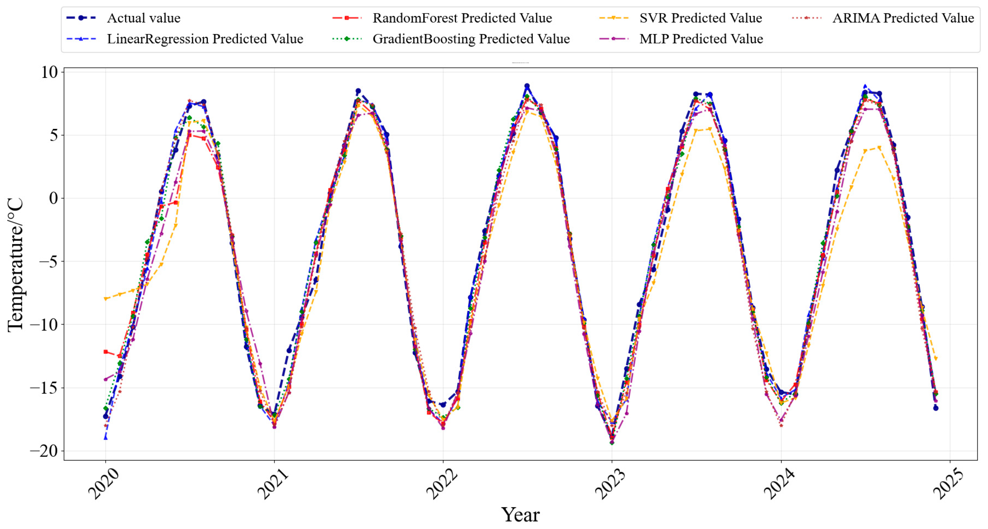
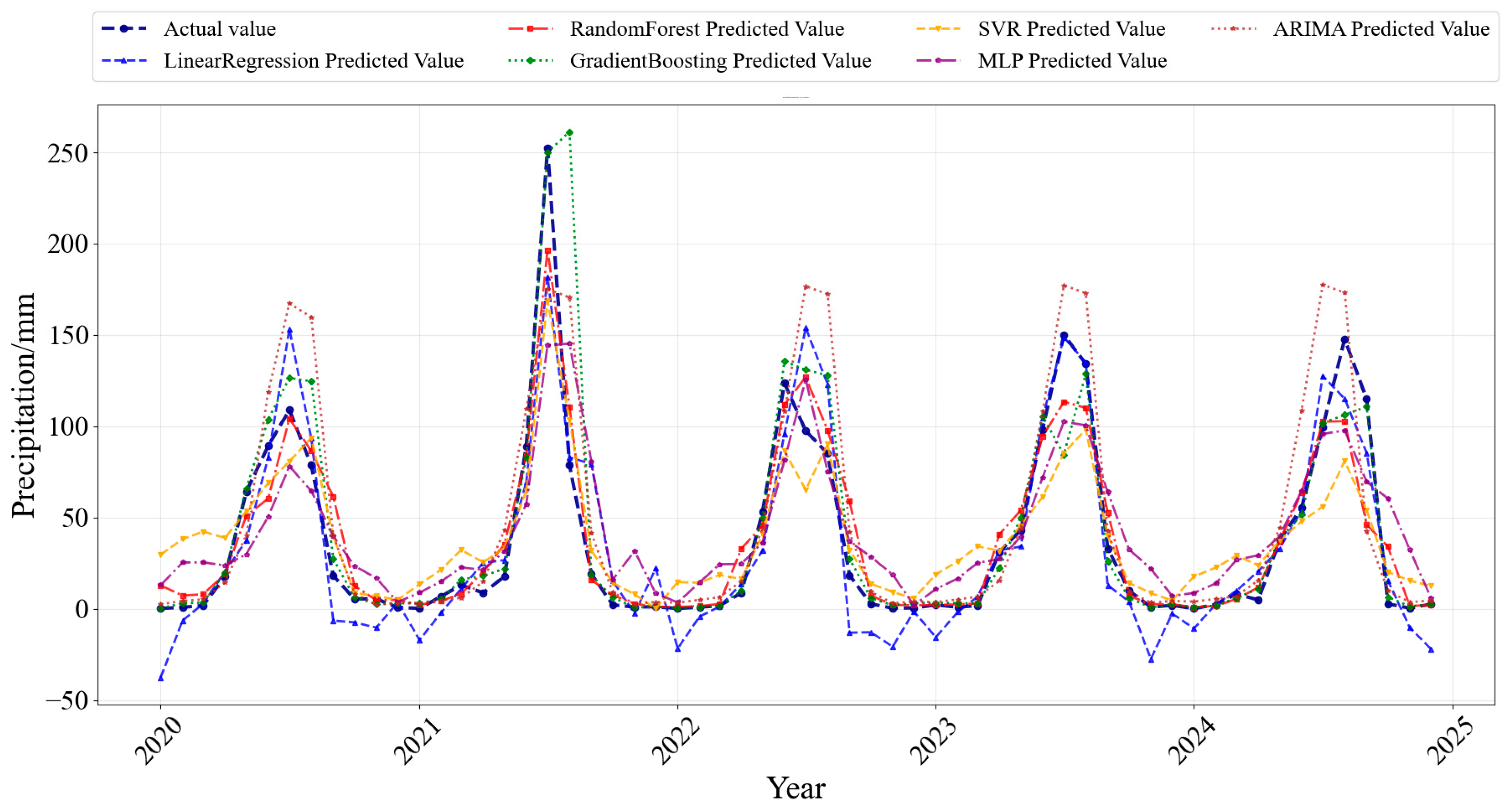
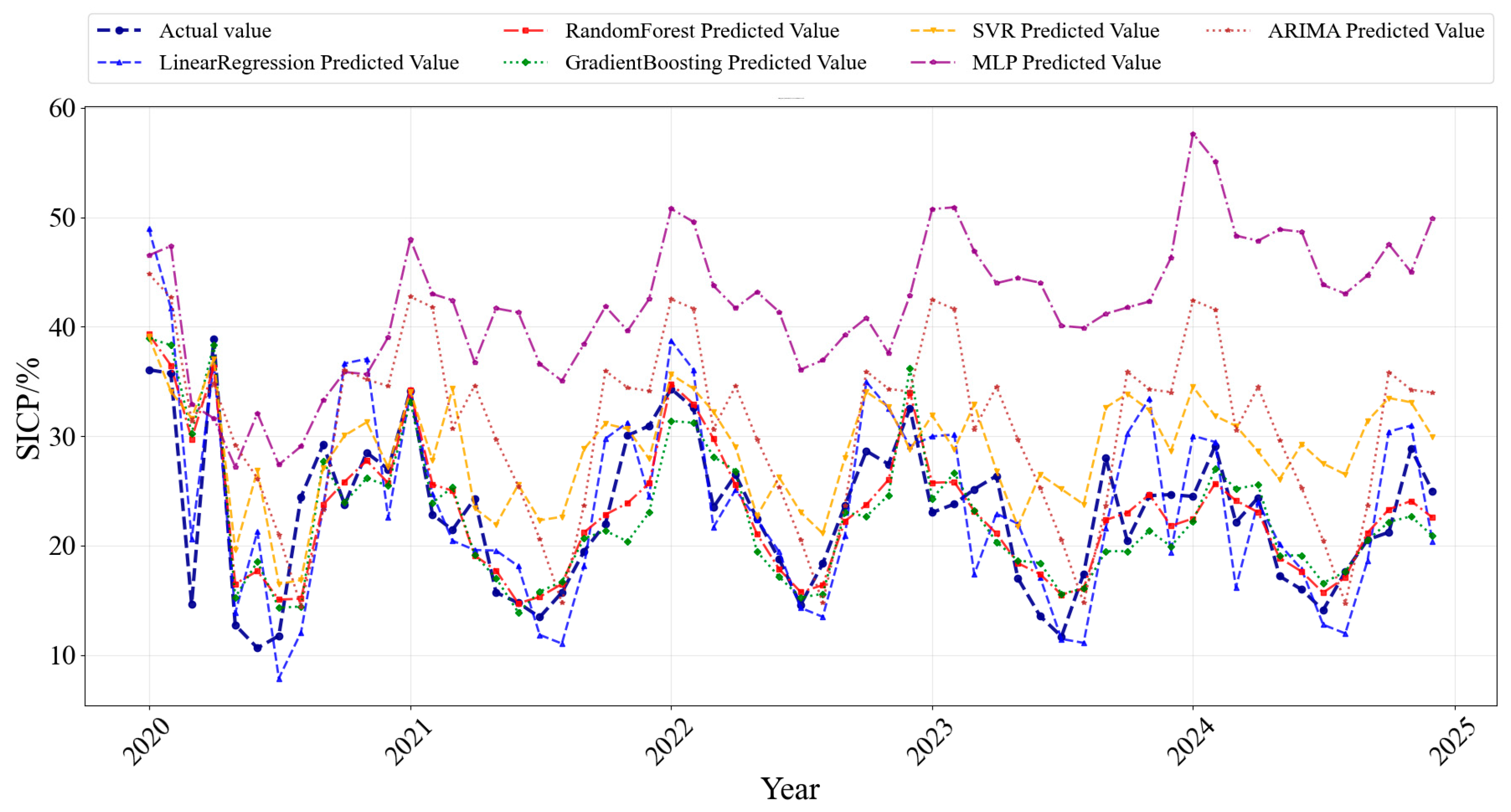
Judging by the models’ fitting performance during the testing period (Figure 11, Figure 12 and Figure 13), there are significant differences in the predictive capabilities of the various algorithms for the three climate variables. For temperature—a variable characterised by relatively strong regularity and low noise—the prediction curves of all models (particularly MLP and random forest) closely align with the actual values, exhibiting the lowest error levels. This indicates that the annual cycle and long-term trend signals in temperature variations have been effectively captured by the models. In contrast, precipitation is more difficult to predict due to the influence of extreme events and high randomness; all models exhibited significant fluctuations in their predictions during the high-precipitation months of summer, although ensemble methods still outperformed linear models in capturing seasonal peaks. As for snow/ice cover, the analysis of prediction errors clearly reveals the temporal characteristics of model performance: during the critical transitional seasons of snow/ice accumulation and melting (such as March–May in spring and October–November in autumn), the errors of all models tend to increase. This reflects the difficulty of statistical models in fully capturing the complex nonlinear physical mechanisms involved in phase transitions. It is worth noting that ensemble models such as random forests and gradient boosting trees generally exhibit more stable and narrower error bands across all variables, validating their advantage in handling complex non-linear relationships and feature interactions; they were therefore selected as the core algorithms for constructing the final ensemble forecast.

4.5.2. Analysis of Temperature Forecasts

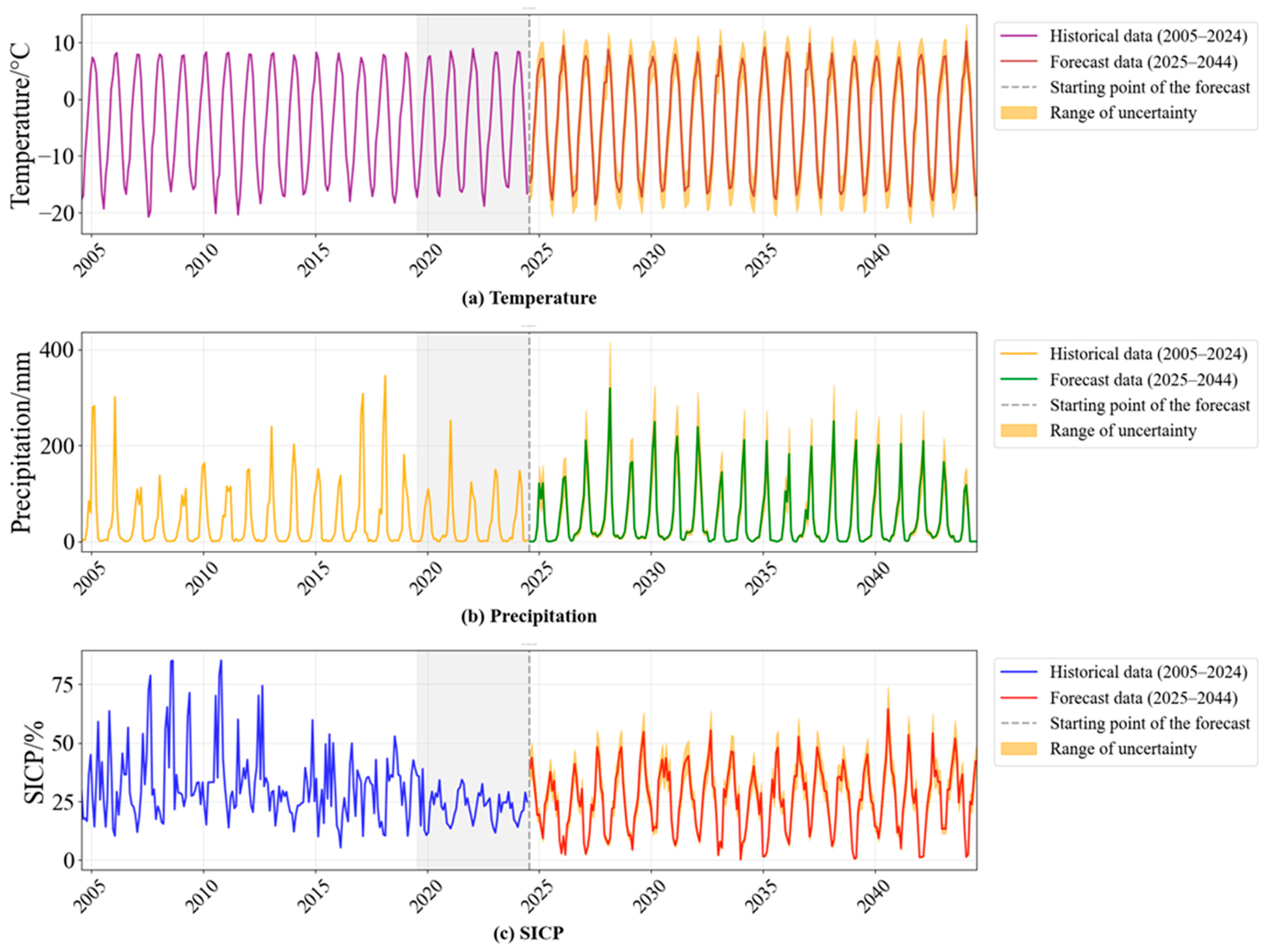
Based on the comparison of model fit in Figure 11 and the quantitative analysis of fit metrics in Table 5, the optimal model was selected: linear regression (MAE = 0.71, RMSE = 0.97, R2 = 0.9880) for the forecast. The temperature model predictions generally show a clear, gradual upward trend, consistent with the context of global warming, with an average annual warming rate of approximately +0.035 °C/year. The warming process is not linear but is accompanied by stable annual cyclical fluctuations; the temperature range during the forecast period is approximately −18.5 to −8.9 °C. The average temperature during the forecast period (2025–2044) is slightly higher than that of the baseline period (2005–2024), characterised by a slight increase in winter lows and a slight rise in summer highs, further exacerbating the seasonal melting of snow/ice and ice. The uncertainty range for the forecast over the next five years is ±1.5 °C.

4.5.3. Analysis of Precipitation Forecasts

Based on the comparison of model fit in Figure 12 and the quantitative analysis of fit metrics in Table 6, the optimal model—random forest (MAE = 11.64, RMSE = 19.10, R2 = 0.8662)—was selected for forecasting. The future precipitation series exhibits a slight ascending trend, with an approximate annual average rate of change of +0.4%, accompanied by relatively mild interannual oscillations. During the forecast period, the annual average precipitation shows a slight increase. The most notable feature is that seasonal variations remain pronounced (high in summer, low in winter), and the model simulates extreme precipitation events with a probability of approximately 8%. Although the overall trend is gradual, the probability of extreme precipitation events will persist. The uncertainty range for the forecast over the next five years is ±15 mm, reflecting the characteristic of sudden fluctuations in precipitation.

4.5.4. Analysis of Snow/Ice Cover Prediction

Based on the comparison of model fit in Figure 13 and the quantitative analysis of fit metrics in Table 7, the optimal model—random forest (MAE = 2.75, RMSE = 3.73, R2 = 0.6973)—was selected for forecasting. The model’s forecast results show that (Figure 14), the snow/ice cover in the study area will generally follow a fluctuating downward trend over the next 20 years. The average annual rate of decline in snow/ice cover during the forecast period is approximately 0.12% per year; by 2044, the average annual snow/ice cover is projected to decrease from 32% during the baseline period (2005–2024) to 29%. Although short-term recoveries may occur due to interannual fluctuations in precipitation (such as in predicted wet years), these cannot reverse the overall long-term downward trend. Furthermore, the uncertainty range for the forecast over the next five years is ±6%, reflecting the impact of interannual variability.
It is worth noting that the R2 values for SVR, MLP and ARIMA on the 2020–2024 test set were −0.31, −8.23 and −1.19, respectively, indicating that these models failed to effectively capture the interannual dynamics of snow/ice cover in the study area during short-term extrapolation. The reasons for the negative R2 values can be summarised in three aspects: firstly, whilst the training and test sets were strictly divided in a continuous time-series manner to ensure no data leakage, the short-term test set (2020–2024) contained a limited number of samples. Furthermore, as snow/ice cover is significantly influenced by seasonal fluctuations and extreme weather events, this led to an amplification of prediction errors when extrapolating using single non-linear and neural network models. Secondly, SVR and MLP are highly sensitive to the scale and non-linear relationships of input features. Given that snow/ice cover exhibits a wide range of interannual fluctuations and pronounced local extremes, this leads to unstable model performance on the test set; thirdly, the ARIMA model assumes a stationary time series, whereas snow/ice cover displays significant seasonal accumulation and long-term non-linear trends. The model is unable to fully capture the superimposed effects of trends and cycles, resulting in limited predictive capability. In contrast, the random forest and gradient boosting models, utilising ensemble learning methods, demonstrate strong robustness to non-linear relationships and local anomalies. With R2 values of 0.697 and 0.615, respectively, on the test set, they exhibit excellent predictive capability, indirectly validating the rationale for this study’s shift towards a multi-model fusion approach capable of capturing complex non-linear relationships.

5. Discussion

5.1. Climate Response Mechanisms and Future Trends in Snow/Ice Cover Changes in the Study Area

Snow/ice cover in the headwaters of the Keriya River is influenced by a combination of meteorological and topographical factors [18]. The region experiences significant temperature fluctuations, extreme precipitation and pronounced topographical variations, resulting in an uneven spatiotemporal distribution of snow/ice cover. As altitude increases, temperatures decrease, and precipitation predominantly takes the form of snow, which promotes the formation and retention of snow/ice cover. Consequently, snow/ice cover in high-altitude areas is more stable and consists mainly of stable snow/ice [41]. Existing research indicates that, compared to precipitation, temperature is the dominant factor influencing snow/ice cover changes [3,42]. In the headwaters of the Keriya River, snow/ice cover exhibits a negative correlation with temperature; however, as altitude increases, this correlation gradually weakens when temperatures fall below 0 °C [43]. Existing research indicates that in high-altitude regions, where temperatures fluctuate below 0 °C throughout the year, snow/ice cover is slow to melt; consequently, minor fluctuations in temperature are unlikely to cause significant changes in snow/ice cover extent [44,45].
On an interannual average, the relationship between snow/ice cover in the upper reaches of the Keriya River and temperature and precipitation is relatively weak, whereas on a monthly scale, the correlation is more pronounced. This phenomenon indicates that the response of snow/ice cover to climatic factors is dependent on the temporal scale [46]. The weaker correlation observed at the annual average scale may be attributed to the mutual cancellation of climatic influences across different seasons during the interannual averaging process. High temperatures and rainfall in spring and summer promote snow/ice melt, resulting in a negative correlation; conversely, low temperatures and snowfall in autumn and winter favour snow/ice accumulation, leading to a positive correlation [47]. This inverse seasonal response is smoothed out at the annual average scale, thereby weakening the overall correlation. In contrast, the monthly scale provides a more detailed insight into the dynamic coupling between snow/ice cover and temperature and precipitation, highlighting the regulatory role of seasonal climatic conditions on snow/ice dynamics. At the monthly scale, changes in temperature and precipitation directly influence snow/ice accumulation and melt, underscoring the critical regulatory role of seasonal climatic conditions in snow/ice dynamics. This regulation does not occur instantaneously; research has shown [48] that there is a lag of approximately one year in the response of upstream flow in the Klyuchevskaya River to changes in minimum temperature, providing quantitative evidence for understanding the physical time lag inherent in snow and ice accumulation and melting processes. Furthermore, seasonal variations in environmental factors such as local topography, radiation balance and wind speed may further amplify or attenuate the effects of temperature and precipitation upon snow/ice cover [49]. The weakening of correlations at the annual average scale does not imply that the influence of climatic factors on snow/ice cover changes is insignificant, but rather reflects the necessity of multi-timescale analysis in elucidating complex hydrometeorological processes.
Forecast sequences for 2025–2044 generated from the optimal model indicate that snow/ice cover may exhibit a slight downward trend, with annual averages below historical averages and earlier snow/ice melt, consistent with the trend of snow/ice melt under global warming [50]. The interannual variability and uncertainty ranges in the projections reflect the influence of climate system variability on snow/ice accumulation. Temperature projections indicate a sustained warming trend, with winter warming likely to exceed that of summer [51]. A study using a coupled model based on the same catchment [52] also indicates that, under the high-emission SSP5-8.5 scenario, future runoff will show an extreme upward trend; from the perspective of hydrological response, this indirectly corroborates the trend of accelerated snow and ice melt predicted in this study. This asymmetric warming may alter the rhythm of snow/ice accumulation and melt. Precipitation forecasts exhibit significant uncertainty and strong interannual variability, but a slight long-term increasing trend suggests that the region may be undergoing a ‘warm-wet’ climate transition [53], wherein rising temperatures enhance the atmosphere’s water-holding capacity, leading to unstable precipitation patterns and an increased risk of extreme precipitation events [54].

5.2. Impact of Declining Snow/Ice Cover on Agricultural Water Resources

A slight decline in snow and ice cover in the headwaters of the Keriya River will have a certain impact on agricultural water resource management in the coming decades. Snow and ice are one of the primary water sources in the region, and their meltwater is crucial for irrigating farmland downstream. As snow and ice cover decrease, and the timing of snowmelt advances, the stability and timing of meltwater supplies may be affected. In response to this trend, it is recommended that farmers consider the following adaptation strategies: Firstly, agricultural water resource management should rely more heavily on real-time meteorological data and climate forecasting software products to ensure early prediction of the snowmelt period. Secondly, water storage and optimised utilisation should be strengthened, and more efficient irrigation systems established to cope with the potential earlier onset of snowmelt. Finally, farmers can adjust crop planting cycles and irrigation volumes according to the characteristics of seasonal climate change, reducing reliance on natural water sources and shifting towards more flexible and sustainable water resource management practices.

5.3. Shortcomings and Limitations

This study has certain limitations, primarily including the inability to effectively distinguish between glaciers and seasonal snow cover. The NDSI threshold method (0.3–0.5) used in this study presents challenges in snow cover extraction, particularly as the spectral characteristics of glacial ice and snow are similar in the visible and short-wave infrared bands, making it difficult for traditional optical remote sensing methods to accurately delineate snow cover extent [55]. This issue is further exacerbated by the presence of 387 modern glaciers (covering a total area of 689 km2) in the study area. This limitation may have two implications for the results. First, snow cover in high-altitude areas (particularly above 5000 m) may be overestimated [56]. Second, glaciers and seasonal snow respond differently to climate change: glacial changes are relatively stable, whereas snow cover fluctuates significantly, and the inconsistency in their trends may affect the attribution analysis of snow dynamics [57], meaning that the observed downward trend in SICP may partly reflect glacial retreat rather than purely seasonal snowpack dynamics. Despite these limitations, through the analysis of long-term remote sensing data, this study effectively reveals the spatiotemporal evolution of overall snow and ice cover in the headwaters of the Keriya River and its comprehensive response to climate change. It provides a crucial foundation for understanding hydrological processes in high-altitude mountainous regions and points the way for future, more detailed studies of snow and ice components.

5.4. Outlook

Future research could be deepened in the following areas: first, by integrating multi-source remote sensing data (such as the Sentinel-1 radar satellite) with machine learning methods (random forests, support vector machines, etc.) to improve the classification accuracy of glaciers and seasonal snow cover, thereby more accurately characterising the true dynamics of snow and ice; second, by applying masking techniques based on glacier inventory data to conduct a zonal analysis of the differentiated responses of snow and ice in glacial and non-glacial areas to climate change; third, by employing terrain-sensitive spatial interpolation methods or multi-source fusion techniques to improve local analysis accuracy, thereby mitigating the potential for false precision and spatial artefacts introduced by the spatial resampling method used in this study. These methods will more precisely capture pixel-level correlations between climate variables and snow/ice cover, avoiding potential errors arising from resampling. Fourth, the multi-model fusion forecasting framework developed in this study will be extended to other high-altitude inland river basins to test its applicability and transferability under different climatic and topographical conditions, thereby providing a more robust methodological foundation and scientific basis for water security and climate change adaptation in arid regions. Fifth, addressing the poor performance of the SVR, MLP and ARIMA models in short-term forecasting, future research will focus on optimising time-series forecasting strategies. We plan to introduce improved lagged features and rolling statistical features, combining periodic and seasonal functions to enhance the models’ sensitivity to non-linearity and seasonal fluctuations. Concurrently, we will explore multi-model weighted forecasting based on ensemble learning and Bayesian Model Averaging (BMA) methods to quantify and correct forecast uncertainty.

6. Conclusions

(1) From 2005 to 2024, the annual average snow/ice cover in the headwaters of the Keriya River showed a non-significant downward trend (−0.69%/year, p > 0.1), peaking in 2009 (43.0%) and reaching a minimum in 2023 (21.5%). Intra-annual variations exhibited a unimodal pattern: January was the peak (average 63.2%), August was the trough (average 11.6%), and September was the only month showing a slight upward trend. The spring melt rate was generally higher than the autumn accumulation rate.
(2) Snow/ice cover percentage increases significantly with altitude: the annual average SCIP in areas below 2000 m is 5.2%; in the 2000–3000 m and 3000–4000 m zones, it rises to 5.7% and 8.3%, respectively, corresponding to the seasonal snow/ice zone; in the 4000–5000 m zone, it rises to 12.4%; in the 5000–6000 m range, it reaches 31.9%, with marked interannual fluctuations (22.5–44.2%); in areas above 6000 m, it is as high as 70.3%, constituting a zone of perennial stable snow/ice cover.
(3) The relationship between snow/ice cover percentage and temperature and precipitation exhibits significant time-scale dependence. On an interannual scale, SCIP exhibits a weak inverse relationship with temperature (R = −0.25) and an exceedingly weak relationship with precipitation (R = −0.14). On a monthly scale, during the melting season (May–August), temperature exerts a dominant negative influence (R = −0.35), whilst during the accumulation season (September–October), precipitation in solid form exerts a positive influence (R = 0.20), with the overall impact of temperature being greater than that of precipitation.
(4) Multi-model ensemble forecasts indicate that during the period from 2025 to 2044, the area of snow/ice cover will show a fluctuating downward trend, with an average annual decline of roughly −0.12%, falling to around 29% by 2044; Temperatures will continue to rise (+0.035 °C/year), with a more pronounced increase in winter; precipitation will increase slightly (+0.4%/year), with summer precipitation still accounting for over 68%. The ranges of uncertainty for the forecasts of each factor are as follows: snow/ice cover ±6%, temperature ±1.5 °C, and precipitation ±15 mm.
To ensure the sustainable use of water resources within the river basin, it is recommended that the management authorities optimise the crop structure in irrigation districts and reservoir regulation strategies in light of the accelerating spring snow/ice melt and the increasing risk of summer flooding, and that they promptly undertake an assessment of water resource carrying capacity against the backdrop of declining snowmelt recharge.

Author Contributions

Conceptualization, W.S. and J.Z.; methodology, W.S. and H.L.; software, W.S. and P.L.; validation, W.S., J.Z. and P.L.; formal analysis, W.S., P.L. and J.Z.; investigation, W.S. and P.L.; resources, W.S. and H.L.; data curation, W.S. and J.Z.; writing—original draft preparation, W.S.; writing—review and editing, K.X.; visualization, W.S. and J.Z.; supervision, K.X. and W.S.; project administration, K.X.; funding acquisition, K.X., J.Z., H.L., W.S. and P.L. All authors have read and agreed to the published version of the manuscript.

Funding

This research was sponsored by the Natural Science Foundation of Xinjiang Uygur Autonomous Region, grant number 2022D01C67.

Institutional Review Board Statement

Not applicable.

Informed Consent Statement

Not applicable.

Data Availability Statement

The original contributions presented in this study are included in the article. Further inquiries can be directed to the corresponding author.

Conflicts of Interest

The authors declare no conflicts of interest.

References

  1. Notarnicola, C. Observing Snow Cover and Water Resource Changes in the High Mountain Asia Region in Comparison with Global Mountain Trends over 2000–2018. Remote Sens. 2020, 12, 3913. [Google Scholar] [CrossRef]
  2. Schöner, W.; Koch, R.; Matulla, C.; Marty, C.; Tilg, A. Spatiotemporal patterns of snow depth within the Swiss–Austrian Alps for the past half century (1961 to 2012) and linkages to climate change. Int. J. Climatol. 2018, 39, 1589–1603. [Google Scholar] [CrossRef]
  3. Ban, C.; Xu, Z.; Zuo, D.; Liu, X.; Zhang, R.; Wang, J. Vertical influence of temperature and precipitation on snow cover variability in the Yarlung Zangbo River basin, China. Int. J. Climatol. 2020, 41, 1148–1161. [Google Scholar] [CrossRef]
  4. Chenggang, Z.; Yaning, C.; Yanjun, C.H.; Meiping, S.U.; Ruifeng, Z.H.; Yang, W.A.; Yuting, L.I. Preliminary report on scientific investigation of water resources on the northern slope of Kunlun Mountains. Arid Land Geogr. 2024, 47, 1097–1105. [Google Scholar]
  5. Yang, Y.; Liu, S.; Xiao, C.; Feng, C.; Li, C. Evaluating Cryospheric Water Withdrawal and Virtual Water Flows in the Tarim River Basin of China: An Input–Output Analysis. Sustainability 2021, 13, 7589. [Google Scholar] [CrossRef]
  6. Yang, C.D.; Xu, M.; Kang, S.C.; Fu, C.S.; Zhang, W.; Hu, D.D. Streamflow abrupt change and the driving factors in glacierised basins of the Tarim Basin, Northwest China. Adv. Clim. Change Res. 2024, 15, 75–89. [Google Scholar] [CrossRef]
  7. Peng, Y.; Kun, X.; Wanqiang, Z.; Sihai, L.; Ling, L. Characteristics of the lagged response of inland river runoff to asymmetric warming on the northern slopes of the Kunlun Mountains [J/OL]. J. Soil Water Conserv. 2026. [Google Scholar] [CrossRef]
  8. Zhang, X.; Li, X.; Li, L.; Zhang, S.; Qin, Q. Environmental factors influencing snowfall and snowfall prediction in the Tianshan Mountains, Northwest China. J. Arid Land 2019, 11, 15–28. [Google Scholar] [CrossRef]
  9. Cowherd, M.; Ruby Leung, L.; Girotto, M. Evolution of global snow drought characteristics from 1850 to 2100. Environ. Res. Lett. 2023, 18, 064043. [Google Scholar] [CrossRef]
  10. Shi, S.; Liu, G. The latitudinal dependence in the trend of the ratio of snow events to precipitation events. Sci. Rep. 2021, 11, 18112. [Google Scholar] [CrossRef]
  11. Gascoin, S.; Luojus, K.; Nagler, T.; Lievens, H.; Masiokas, M.; Jonas, T.; Zheng, Z.; De Rosnay, P. Remote sensing of mountain snow from space: Status and recommendations. Front. Earth Sci. 2024, 12, 1381323. [Google Scholar] [CrossRef]
  12. Li, X.; Jing, Y.; Shen, H.; Zhang, L. Recent developments in cloud removal approaches for the MODIS snow cover product. Hydrol. Earth Syst. Sci. 2019, 23, 2401–2416. [Google Scholar] [CrossRef]
  13. Qin, S.; Xiao, P.; Zhang, X. How do snow cover fractions change and respond to climate in the Altai Mountains of China? Int. J. Climatol. 2022, 42, 7213–7227. [Google Scholar] [CrossRef]
  14. Wufu, A.; Chen, Y.; Yang, S.; Lou, H.; Wang, P.; Li, C.; Wang, J.; Ma, L. Changes in glacial meltwater runoff and its response to climate change in the Tianshan region detected using unmanned aerial vehicles (UAVs) and satellite remote sensing. Water 2021, 13, 1753. [Google Scholar] [CrossRef]
  15. Liu, Y.; Xu, J.; Lu, X.; Nie, L. Assessment of glacier- and snowmelt-driven streamflow in the arid middle Tianshan Mountains of China. Hydrol. Process. 2020, 34, 2750–2762. [Google Scholar] [CrossRef]
  16. Wang, Y.F. Climate and Snow Cover Changes in the Keriya River Basin and Their Impact on Runoff; Xinyang Normal University: Xinyang, China, 2024. [Google Scholar] [CrossRef]
  17. Blau, M.T.; Kad, P.; Turton, J.V.; Ha, K.J. Uneven global retreat of persistent mountain snow cover alongside mountain warming from ERA5-land. npj Clim. Atmos. Sci. 2024, 7, 278. [Google Scholar] [CrossRef]
  18. Yan, W.; Wang, Y.; Ma, X.; Liu, M.; Yan, J.; Tan, Y.; Liu, S. Snow cover and climate change and their coupling effects on runoff in the Keriya River Basin during 2001–2020. Remote Sens. 2023, 15, 3435. [Google Scholar] [CrossRef]
  19. Niu, S.; Sun, M.; Wang, G.; Wang, W.; Yao, X.; Zhang, C. Glacier Change and Its Influencing Factors in the Northern Part of the Kunlun Mountains. Remote Sens. 2023, 15, 3986. [Google Scholar] [CrossRef]
  20. Roy, D.P.; Wulder, M.A.; Loveland, T.R.; Ce, W.; Allen, R.G.; Anderson, M.C.; Helder, D.; Irons, J.R.; Johnson, D.M.; Kennedy, R.; et al. Landsat-8: Science and product vision for terrestrial global change research. Remote Sens. Environ. 2014, 145, 154–172. [Google Scholar] [CrossRef]
  21. Sulla-Menashe, D.; Friedl, M.A.; Woodcock, C.E. Sources of bias and variability in long-term Landsat time series over Canadian boreal forests. Remote Sens. Environ. 2016, 177, 206–219. [Google Scholar] [CrossRef]
  22. Peng, S.; Ding, Y.; Liu, W.; Li, Z. 1 km monthly temperature and precipitation dataset for China from 1901 to 2017. Earth Syst. Sci. Data 2019, 11, 1931–1946. [Google Scholar] [CrossRef]
  23. Ding, Y.; Peng, S. Spatiotemporal trends and attribution of drought across China from 1901–2100. Sustainability 2020, 12, 477. [Google Scholar] [CrossRef]
  24. Kumar, B.; Lakshmi, V.; Patra, K.C. Evaluating the uncertainties in the SWAT model outputs due to DEM grid size and resampling techniques in a large Himalayan—River basin. J. Hydrol. Eng. 2017, 22, 04017039. [Google Scholar] [CrossRef]
  25. Stillinger, T.; Roberts, D.A.; Collar, N.M.; Dozier, J. Cloud masking for Landsat 8 and MODIS Terra over snow-covered terrain: Error analysis and spectral similarity between snow and cloud. Water Resour. Res. 2019, 55, 6169–6184. [Google Scholar] [CrossRef] [PubMed]
  26. Qiu, S.; Zhu, Z.; He, B. Fmask 4.0: Improved cloud and cloud shadow detection in Landsat 4–8 and Sentinel-2 imagery. Remote Sens. Environ. 2019, 231, 111205. [Google Scholar] [CrossRef]
  27. Poussin, C.; Timoner, P.; Chatenoux, B.; Giuliani, G.; Peduzzi, P. Improved Landsat-based snow cover mapping accuracy using a spatiotemporal NDSI and generalised linear mixed model. Sci. Remote Sens. 2023, 7, 100078. [Google Scholar] [CrossRef]
  28. Gascoin, S.; Grizonnet, M.; Bouchet, M.; Salgues, G.; Hagolle, O. Theia Snow collection: High-resolution operational snow cover maps from Sentinel-2 and Landsat-8 data. Earth Syst. Sci. Data 2019, 11, 493–514. [Google Scholar] [CrossRef]
  29. Roessler, S.; Dietz, A.J. Development of Global Snow Cover—Trends from 23 Years of Global SnowPack. Earth 2022, 4, 1–22. [Google Scholar] [CrossRef]
  30. Yan, D.; Zhang, Y.; Gao, H. Development of a Daily Cloud-Free Snow-Cover Dataset Using MODIS-Based Snow-Cover Probability for High Mountain Asia during 2000–2020. Remote Sens. 2024, 16, 2956. [Google Scholar] [CrossRef]
  31. Sharma, J.; Singh, O. Variability and time series trend analysis of streamflow in response to climatic and anthropogenic factors over the Narmada River basin, India. Sustain. Water Resour. Manag. 2024, 10, 75. [Google Scholar] [CrossRef]
  32. Zhao, Q.; Hao, X.; Wang, J.; Luo, S.; Shao, D.; Li, H.; Feng, T.; Zhao, H. Changes in snow cover phenology and its response to climate in China during 2000–2020. Remote Sens. 2022, 14, 3936. [Google Scholar] [CrossRef]
  33. Hodson, T.O. Root Mean Square Error (RMSE) or Mean Absolute Error (MAE): When to Use them or Not; Copernicus GmbH: Göttingen, Germany, 2022. [Google Scholar] [CrossRef]
  34. Chicco, D.; Warrens, M.J.; Jurman, G. The coefficient of determination R-squared is more informative than SMAPE, MAE, MAPE, MSE and RMSE in regression analysis evaluation. PeerJ Comput. Sci. 2021, 7, e623. [Google Scholar] [CrossRef]
  35. Iyeme, E.E.; Ekah, U.J.; Njok, A.O.; Agbo, E.P.; Offorson, G.C. Trend Analysis of Climate Change across Nigeria: A Mann-Kendall and Sen’s Approach. Arch. Curr. Res. Int. 2024, 24, 450–467. [Google Scholar] [CrossRef]
  36. Notaro, V.; Liuzzo, L.; Freni, G. A BMA Analysis to Assess the Urbanisation and Climate Change Impact on Urban Watershed Runoff. Procedia Eng. 2016, 154, 868–876. [Google Scholar] [CrossRef]
  37. Unnikrishnan, P.; Jothiprakash, V. Extraction of Nonlinear Rainfall Trends Using Singular Spectrum Analysis. J. Hydrol. Eng. 2015, 20, 05015007. [Google Scholar] [CrossRef]
  38. Gharib, A.; Davies, E.G.; Goss, G.G.; Faramarzi, M. Assessment of the combined effects of threshold selection and parameter estimation of the Generalised Pareto Distribution with applications to flood frequency analysis. Water 2017, 9, 692. [Google Scholar] [CrossRef]
  39. Hernández-Henríquez, M.A.; Déry, S.J.; Derksen, C. Polar amplification and elevation-dependence in trends of Northern Hemisphere snow cover extent, 1971–2014. Env. Res. Lett. 2015, 10, 044010. [Google Scholar] [CrossRef]
  40. Ma, Q.; Keyimu, M.; Li, X.; Wu, S.; Zeng, F.; Lin, L. Climate and elevation control snow depth and snow phenology on the Tibetan Plateau. J. Hydrol. 2023, 617, 128938. [Google Scholar] [CrossRef]
  41. Yan, W.; Wang, Y.; Ma, X.; Tan, Y.; Yan, J.; Liu, M.; Liu, S. What Is the Threshold Elevation at Which Climatic Factors Determine Snow Cover Variability? A Case Study of the Keriya River Basin. Remote Sens. 2023, 15, 4725. [Google Scholar] [CrossRef]
  42. Tang, Z.; Wang, X.; Wang, J.; Wang, X.; Li, H.; Jiang, Z. Spatiotemporal Variation of Snow Cover in the Tianshan Mountains, Central Asia, Based on the Cloud-Free MODIS—Fractional Snow Cover Product, 2001–2015. Remote Sens. 2017, 9, 1045. [Google Scholar] [CrossRef]
  43. Wu, S.; Zhang, X.; Du, J.; Zhou, X.; Tuo, Y.; Li, R.; Duan, Z. The vertical influence of temperature and precipitation on snow cover variability in the Central Tianshan Mountains, Northwest China. Hydrol. Process. 2019, 33, 1686–1697. [Google Scholar] [CrossRef]
  44. Zhang, Y.; Gulimire, H.; Sulitan, D.; Hu, K. Monitoring and analysis of snow cover change in an alpine mountainous area in the Tianshan Mountains, China. J. Arid Land 2022, 14, 962–977. [Google Scholar] [CrossRef]
  45. Jiang, X.; Chen, H.; Tang, Z.; Guo, H.; Deng, G.; You, Y.; Hou, H. Temperature Governs the Elevation Dependency of Snow Cover Changes in the Upper Reaches of the Yarkand River Basin. Remote Sens. 2025, 18, 80. [Google Scholar] [CrossRef]
  46. Qiao, X.; Liu, J.; Wang, S.; Wang, J.; Ji, H.; Chen, X.; Liu, H.; Lu, F. Lead-lag correlations between snow cover and meteorological factors at multi-time scales in the Tibetan Plateau under climate warming. Theor. Appl. Clim. 2021, 146, 1459–1477. [Google Scholar] [CrossRef]
  47. Wang, X.; Wu, C.; Wang, H.; Gonsamo, A.; Liu, Z. No evidence of widespread decline of snow cover on the Tibetan Plateau over 2000–2015. Sci. Rep. 2017, 7, 14645. [Google Scholar] [CrossRef]
  48. Xing, K.; Wang, J.; Liu, S. Study on the coupling mechanism and dynamic response of hydrometeorological factors and runoff in the upper reaches of the Kriya River based on the SVAR model. J. Hydrol. Reg. Stud. 2026, 65, 103467. [Google Scholar] [CrossRef]
  49. Li, J.; Li, S.; Pi, H. Interaction effects of various impact factors on snow in the Yangtze and Yellow River headwater regions, China. Ecol. Indic. 2024, 166, 112330. [Google Scholar] [CrossRef]
  50. Guo, Y.; Yang, Y.; Yang, D.; Zhang, L.; Zheng, H.; Xiong, J.; Ruan, F.; Han, J.; Liu, Z. Warming leads to both earlier and later snowmelt floods over the past 70 years. Nat. Commun. 2025, 16, 3663. [Google Scholar] [CrossRef]
  51. Suonan, J.; Classen, A.T.; Zhang, Z.; He, J. Asymmetric winter warming advanced plant phenology to a greater extent than symmetric warming in an alpine meadow. Funct. Ecol. 2017, 31, 2147–2156. [Google Scholar] [CrossRef]
  52. Xing, K.; Yang, P.; Liu, S.; Zhao, Q. A Coupled SWAT-LSTM Approach for Climate-Driven Runoff Dynamics in a Snow-and Ice-Fed Arid Basin. Sustainability 2025, 17, 10235. [Google Scholar] [CrossRef]
  53. Yang, J.; Zhang, Q.; Lu, G.; Liu, X.; Wang, Y.; Wang, D.; Liu, W.; Yue, P.; Zhu, B.; Duan, X. Climate transition from warm-dry to warm-wet in Eastern Northwest China. Atmosphere 2021, 12, 548. [Google Scholar] [CrossRef]
  54. Gu, L.; Yin, J.; Gentine, P.; Wang, H.M.; Slater, L.J.; Sullivan, S.C.; Chen, J.; Zscheischler, J.; Guo, S. Large anomalies in future extreme precipitation sensitivity driven by atmospheric dynamics. Nat. Commun. 2023, 14, 3197. [Google Scholar] [CrossRef]
  55. Ji, W.; Hao, X.; Shao, D.; Yang, Q.; Wang, J.; Li, H.; Huang, G. A New Index for Snow/Ice/Ice-Snow Discrimination Based on BRDF Characteristic Observation Data. J. Geophys. Res. Atmos. 2022, 127, e2021JD035742. [Google Scholar] [CrossRef]
  56. Smitha, P.S.; Maya, K.; Sudheer, K.P.; Bindhu, V.M.; Sreelash, K.; Padmalal, D. A novel approach for the separation of frozen water bodies from snow to enhance snow mapping accuracy in high-altitude wetlands. Cold Reg. Sci. Technol. 2025, 240, 104649. [Google Scholar] [CrossRef]
  57. Yang, Z.L.; Bai, P. Response of runoff and its components to climate change in the Manas River of the Tian Shan Mountains. Adv. Clim. Change Res. 2024, 15, 62–74. [Google Scholar] [CrossRef]
Figure 1. Overview map of the headwaters of the Keriya River.
Sustainability 18 05385 g001
Figure 2. Monthly variation in SICP in the headwaters of the Keriya River.
Sustainability 18 05385 g002
Figure 3. Seasonal variations in SICP in the headwaters of the K River.
Sustainability 18 05385 g003
Figure 4. Interannual variation in SICP in the headwaters of the Keriya River.
Sustainability 18 05385 g004
Figure 5. Monthly-scale interannual variations in SICP in the headwaters of the Keriya River.
Sustainability 18 05385 g005
Figure 6. Interannual variations in seasonal SICP in the headwaters of the Keriya River.
Sustainability 18 05385 g006
Figure 7. Interannual variations in SICP across elevation zones in the headwaters of the Keriya River.
Sustainability 18 05385 g007
Figure 8. Intra-annual (a) and interannual (b) temperature variations in the headwaters of the Keriya River.
Sustainability 18 05385 g008
Figure 9. Intra-annual (a) and interannual (b) variations in precipitation in the headwaters of the Keriya River.
Sustainability 18 05385 g009
Figure 10. Heatmap of correlations between SICP and meteorological factors.
Sustainability 18 05385 g010
Figure 11. Comparison of simulated and observed air temperatures in the headwaters of the Keriya River, 2020–2024.
Sustainability 18 05385 g011
Figure 12. Comparison of simulated and observed precipitation in the headwaters of the Keriya River, 2020–2024.
Sustainability 18 05385 g012
Figure 13. Comparison of SICP simulations and observed data for the headwaters of the Keriya River, 2020–2024.
Sustainability 18 05385 g013
Figure 14. Historical time series and trend forecasts for air temperature, precipitation and snow/ice cover in the headwaters of the Klyar River.
Sustainability 18 05385 g014
Table 1. Data for the study area.
Data TypeData Product/NameSource Organisation and PlatformTime RangeSpatial Resolution
Remote Sensing DataLandsat 7 ETM+ Level-1US Geological Survey (USGS) Earth Explorer (https://earthexplorer.usgs.gov/)2005–201330 m (Path 149/Row 34)
Landsat 8 OLI/TIRS Level-1US Geological Survey (USGS) Earth Explorer (https://earthexplorer.usgs.gov/)2013–202430 m (Path 149/Row 34)
Meteorological dataMonthly precipitation and temperatureNational Earth System Science Data Centre (http://www.geodata.cn, accessed on 19 February 2025)2005–20241 km (uniformly resampled to 30 m)
DEM DataSRTM DEM V4.1Geospatial Data Cloud Platform (http://www.gscloud.cn/, accessed on 20 February 2025)90 m (uniformly resampled to 30 m)
Table 2. Area statistics for elevation zones in the headwaters of the Keriya River.
Elevation Interval (m)Area (km2)
≤200063.31
2000–30001595.38
3000–40001459.82
4000–50005579.16
5000–60006859.44
≥6000793.72
Table 3. Statistical analysis of seasonal SICP monthly combinations in the headwaters of the Keriya River basin.
SeasonGroupCorresponding MonthsSICP (%)Seasonal Average (%)
SpringA (early)March29.630.6
B (mid-season)April34.3
C (late)May27.8
SummerA (early)June23.820.3
B (mid-season)July19.9
C (late)August17.4
AutumnA (early)September25.131.0
B (mid)October33.9
C (late)November34.0
WinterA (early)December33.438.1
B (mid-term)January40.0
C (late)February39.8
Table 4. Monthly correlation table for snow/ice cover, temperature and precipitation.
M.Jan.Feb.Mar.Apr.May.Jun.Jul.Aug.Sep.Oct.Nov.Dec.
Tem.0.003−0.0300.020−0.1300.310−0.300.023−0.350−0.5000.450−0.170−0.020
Pre.0.3400.340−0.310−0.440−0.1100.130−0.0800.2600.1700.200−0.370−0.070
Table 5. Results of multi-model performance evaluation for temperature.
ModelR2MAERMSE
Linear Regression0.98800.710.97
Gradient Boosting0.98700.821.01
ARIMA0.98101.011.22
Random Forest0.97591.031.38
MLP0.96601.311.64
SVR0.90872.022.68
Table 6. Results of multi-model performance evaluation for precipitation.
ModelR2MAERMSE
Random Forest0.866211.6419.10
Linear Regression0.819316.0622.20
SVR0.748219.8726.21
Gradient Boosting0.719610.0827.66
MLP0.687422.3029.20
ARIMA0.628718.8931.83
Table 7. Performance evaluation results of the SICP multi-model.
ModelR2MAERMSE
Random Forest0.69732.753.73
Gradient Boosting0.61473.094.20
Linear Regression0.32604.525.56
SVR0.00006.477.74
MLP0.000019.3120.57
ARIMA0.00008.9210.03
Disclaimer/Publisher’s Note: The statements, opinions and data contained in all publications are solely those of the individual author(s) and contributor(s) and not of MDPI and/or the editor(s). MDPI and/or the editor(s) disclaim responsibility for any injury to people or property resulting from any ideas, methods, instructions or products referred to in the content.