Article

A Novel Inland Barge Practice for Sustainable Freight in the Pearl River Delta: Pricing Strategies for Outsourcing Leftover Shipping Demands

1
Department of Electronic Business, South China University of Technology, Guangzhou 510006, China
2
Logistics and Supply Chain Management Programme, School of Business, Singapore University of Social Sciences, Singapore 599494, Singapore
*
Author to whom correspondence should be addressed.
Sustainability 2026, 18(11), 5304; https://doi.org/10.3390/su18115304
Submission received: 1 April 2026 / Revised: 14 May 2026 / Accepted: 18 May 2026 / Published: 25 May 2026
(This article belongs to the Special Issue Green and Smart Synergies in Port, Shipping and Water Transportation)

Abstract

The Pearl River Delta region suffers from congestion in the urban road network, noise, air pollution, and other “urban diseases”. Vigorously developing inland water transportation can greatly alleviate these “urban diseases”. However, it is difficult to take advantage of the inland waterway transportation cost advantages due to the Pearl River Delta’s short haul distance characteristics. In recent business practice, a novel, environment-friendly, and competitiveness-enhanced inland waterway transportation mode has emerged in the area, called the leftover-cargo mode in this paper. This mode is composed of first-tier (big companies) and second-tier (small companies) inland barge companies, which establish a cooperative relationship and jointly meet the needs of shippers and can lead to a modal shift from inland truck to inland waterway transportation. In real practice, the pricing methods of this novel mode still rely on experience. We propose four pricing game theory models based on channel leadership in order to investigate how decision-making impacts the pricing and income of the two-tier companies. We find that, if the market price ceiling is low, second-tier inland barge companies always benefit more than first-tier companies, which is very interesting and counter to the existing literature. These findings offer pricing insights into economically viable leftover-cargo cooperation and its role in supporting sustainable road-to-waterway freight modal shift in the Pearl River Delta.

1. Introduction and Background

In recent decades, with the continuing development of industrial economies, greenhouse gas emissions have continued to rise, which has brought irreversible damage to the global climate. In 2008, the UK promulgated the “Climate Change Act”, becoming the first developed country in the world to set a legislative target of achieving zero carbon emissions by 2050. Since then, developed countries (including the United States, Germany, France, and Japan) have also committed to achieving zero carbon emissions by 2050. In 2020, at the seventy-fifth UN General Assembly, the Chinese government also promised that “China will strive to reach the peak of carbon dioxide emissions by 2030, and strive to achieve carbon neutrality by 2060.” In order to achieve this goal, the Chinese government has issued a variety of policies and measures, including a proposal to expand the effectiveness of the infrastructure and to continue promoting a modal shift from truck to barge transportation of bulk cargo in ports.
China’s Pearl River Delta region has three world-renowned gateway seaports, namely Shenzhen Port (4th), Guangzhou Port (6th), and Hong Kong Port (12th) (ranking in 2024 in terms of annual throughput). Around 70 million containers are assembled in this region every year, and most of the intermodal mode depends on trucks, which has led to congestion in the urban road network, noise, and air pollution in this region. Actively developing inland waterway transportation can greatly alleviate these “urban diseases”. Recent studies further indicate that inland waterway transport plays a critical role in facilitating freight modal shift from road to more sustainable transport modes [1]. As the average haul distance of inland waterway transportation in the Pearl River Delta is only 224.2 km, it is difficult to take advantage of its cost advantages. Therefore, the development of inland waterway transportation, an environmentally friendly and competitiveness-enhanced transportation mode, urgently requires business model innovation. This region is rich in inland waterway resources and has a more open market economy foundation, and these conditions can provide a good soil for the reform and innovation of the inland waterway transportation market in the Pearl River Delta region. The status quo here is that, in addition to large barge companies, there are many small barge companies engaged in short-distance inland waterway transportation from coastal ports to inland river ports throughout the region. In 2023, the annual inland water freight volume of the Pearl River system exceeded 1.5 billion tons, an increase from the previous year of 7.9% [2]. Although the huge inland barge freight volume brings attractive economic benefits already, it has large potential to be promoted due to its low utilization ratio, especially compared with the inland truck intermodal mode.
With the increasing severity of environmental problems, low-carbon development has become an inevitable choice. As we know, inland waterway transportation is recognized as more economical and environmentally friendly than inland truck transportation, and it can help to reduce road congestion in crowded areas [3,4,5]. A research article suggested that the development of railway infrastructure in China could effectively reduce haze pollution [6]. Moreover, compared with trains, barges do not need to build as much infrastructure. So, vigorously developing inland waterway transportation is both essential and holds the promise to reduce carbon emissions. Water transportation is notably more efficient at handling large-volume cargoes and consumes less energy. Consequently, the greater the volume of bulk freight tasks shifted from roadway to water transportation, the more pronounced the benefits of this mode shift become [7]. In fact, since 2010, the proportion of freight transported by train has decreased significantly. At the same time, with the implementation of the 14th Five-Year Plan, the navigable mileage of inland barge channels has increased constantly [8], which is conducive to the further development of inland waterway transportation. The market share of inland waterway transportation has not significantly improved, however. One reason is that barges are in fierce competition with trucks, as cost and time are regarded as the main factors in shippers’ selection of carriers [9]. Tiwari et al. [10] have proved that shippers’ unwillingness to choose barges rises if the transport time is too long. Barges do enjoy a cost advantage over trucks for shippers [3], but inland container ships are mostly of fixed specification (which is difficult to change in the short term), and thus the fixed cost per voyage is relatively high. In order to ensure profits, most inland barge companies pursue a high load strategy, but this extends the cargo collection time and makes it impossible to respond to market demand in a timely manner, thereby causing losses [11]. In addition, the cost advantages of inland waterway transportation are less obvious to some extent due to the short distances traversed. Shippers (having formed the impression that barges cannot meet their demand) will not consider inland barges later, but will choose trucks instead. This further reduces the scale of inland waterway transportation utilization to a low level.
Decreasing the cargo collection time in order to improve market responsiveness has thus become the key factor in the development of inland waterway transportation. Traditional approaches to the problem include increasing the frequency and number of ships dispatched, and learning from the maritime industry in order to build strategic alliances or to effect slot exchanges. An increase in the number of vessels available may improve barge transportation market share, but it has the disadvantage of high input costs, which small companies may not be able to afford. Moreover, an excessive number of vessels may lead to berth and landside handling bottlenecks [12]. At the network level, inland waterway congestion and inefficient vessel scheduling can further create bottlenecks, jointly increasing cargo collection time and weakening the time competitiveness of barge transport [13]. Strategic alliances (the joint operation of container ships through cooperation in decisions related to ship type, ship number, navigation plans, etc.) represent an alternative for barge companies [14]. This is not a foolproof strategy for increasing market share, however, as alliance members may sacrifice the interests of the alliance or other members in order to maximize their individual interest at any given time [15]. Slot exchange is a two-way, slot transaction relationship between two liner companies; that is, one company sells a given slot to the other and simultaneously purchases a slot in return. Yang et al. [16] conclude that slot exchange can improve both the efficiency of ship capacity utilization (without changing the total amount of tonnage), and more flexibly respond to different freight demands (thereby increasing a liner company’s revenue through ensuring customer satisfaction). They also point out, however, that slot exchange has similar shortcomings to the strategic alliances mentioned before. In other words, due to fierce competition for resources in the inland barge market, cooperation between inland barge companies may lead to the loss of their own customers through poaching. Therefore, the above three traditional methods of improving barge efficiency have had only a limited effect in improving the market responsiveness of inland waterway transportation. Similar concerns have been examined in international studies on intermodal and inland waterway transport. Caris et al. [17] review decision-support models for intermodal freight transport, highlighting coordination and planning problems across transport modes. Konings [18] analyzes container barge transport around the Port of Rotterdam and shows its role in improving hinterland accessibility. These studies indicate that the challenges of modal shift, barge capacity utilization, and road–waterway coordination are shared across different inland transport systems.
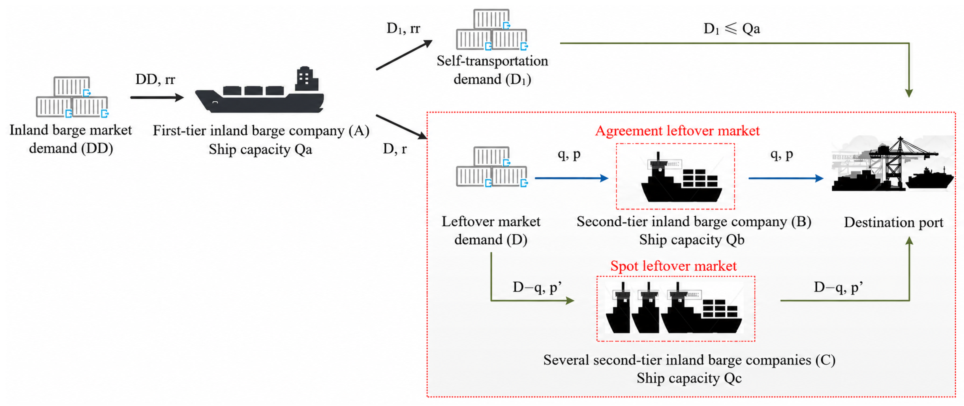
In this paper, we describe an interesting phenomenon found through industry experimentation, and which we believe shows promise in ameliorating some of the challenges to greater barge utilization in cargo shipping. In China’s Pearl River Delta, inland barge companies are generally divided into two categories—we call them first-tier inland barge companies (FTCs) and second-tier inland barge companies (STCs). FTCs undertake the lion’s share of transportation orders from shipping companies, while STCs use smaller ships to transport containers that exceed the shipping capacity of FTCs. When an FTC collects containers from the market and acquires containers beyond the firm’s shipping capacity, the surplus containers will be delivered to an STC for transportation. Notably (and in contrast to slot exchange), STCs do not deal with shippers directly. Rather, an STC signs transportation agreements with FTCs, ensuring that there will be no seizure of customers during the period of ostensible cooperation. An FTC then only needs to pay the contracted price for the shipping space from STCs, allowing it to charge a stable price and deliver excellent service to customers. Industry professionals call this transaction the “leftover-cargo mode”. The leftover-cargo mode effectively breaks the structural restrictions on the shipping capacity of the barge companies, shortens the cargo collection times for inland waterway transportation, and improves the overall competitiveness of barges compared with trucks. At the same time, the leftover-cargo mode has the further advantages of increasing customer loyalty while decreasing unit costs. The leftover-cargo mode is thus conducive to solving the development dilemma of the container transport industry in the Pearl River Delta: reducing environmental pollution while ensuring economic benefits. The operation process of the leftover-cargo mode is shown in Figure 1.
Since the leftover-cargo mode is an emerging transportation service, the pricing methods still rely on industry experience rather than any scientific basis. This mode, however, has the potential to solve the problem of inland barge company pricing decisions. We believe that, by providing a broadly applicable model for viable price strategies within the leftover-cargo mode, we can provide a foundation for its expansion outside of the Pearl River Delta. The spread of this mode, in turn, can engage more companies in the market, enhance the overall competitiveness of inland waterway transportation, and reduce the total carbon emissions of cargo transportation.
In the leftover-cargo mode, an FTC obtains revenue from shippers by transporting containers from port, and then pays an additional shipping space purchase fee to the contracted STCs. STCs and FTCs then jointly transport the shippers’ containers. This paper considers a game theory-based, secondary port supply chain composed of one FTC and one STC operating on the same shipping route. This one-FTC/one-STC structure is used as a benchmark setting, which is widely adopted in related pricing and supply-chain studies because it makes the strategic interaction transparent while retaining the essential contractual relationship between the two parties [19,20,21]. It should therefore be understood as a simplified analytical setting rather than as a complete description of the whole Pearl River Delta market. The novelty of this study does not lie in using Stackelberg, Nash, or centralized games per se, but in applying these pricing structures to the leftover-cargo mode, an emerging horizontal residual-capacity cooperation mechanism in the inland barge market. Unlike conventional vertical supply-chain pricing settings, the FTC and STC jointly provide the same transport service; the STC does not directly contract with shippers, the agreed volume links pricing with capacity sharing, and the shipper-facing market price is constrained by truck competition. In our model, the FTC selects the market price and the agreed volume, and the STC determines the agreed price. Based on the differences in channel leadership, four game theory models of pricing are developed: the FTC-Stackelberg model (F), the STC-Stackelberg model (S), the Nash model (N), and the centralized model (C).
In addition, it must be taken into account that the FTC cannot allow the market price to rise without any limit. Since trucks and barges are fungible, price is one of the primary factors in barges gaining a competitive advantage [3]; thus, the market price of barges cannot exceed the transport price of trucks. That is, a market price ceiling exists. In the benchmark case study, the market price ceiling r * is approximated by the average truck freight rate over the same origin–destination distance. This is a benchmark approximation rather than a universal shipment-level ceiling, because actual truck freight rates may vary with shipment urgency, seasonality, fuel prices, operator type, and contract conditions. However, as this paper focuses on the agreement leftover market on a fixed route with relatively stable demand and long-term capacity arrangements, a route-level average truck rate is used to capture the main intermodal substitution pressure in a tractable way. This paper will consider this point in the models and further explore the effects of a market price ceiling on optimal decisions. We aim to discuss three problems: (i) What is the influence of channel leadership on optimal pricing decisions and supply chain performance? (ii) What influence do the agreed price and the market price ceiling have on the optimal decisions and performance of each model? (iii) Among the four types of leadership, which one is the best from the perspective of each market participant?
Our paper is organized as follows: Section 2 reviews the related literature. Then, we present four game theory models based on channel leadership and deduce the equilibrium outcomes in Section 3. Section 4 makes a comparative, numerical analysis of equilibrium outcomes under the different models. Section 5 presents a case study and analytically investigates the influence of channel leadership, the agreed price, and the market price ceiling. Section 6 summarizes the conclusions and discusses the results.

2. Literature Review

In actual operation, empirical pricing is utilized in this novel leftover-cargo mode. This approach, however, relies too much on experience and lacks theoretical research that could help the mode to expand to other regions, because this new mode has just emerged in the industry in recent years. In this paper, we propose four game theory pricing models based on channel leadership in order to study how decision-making impacts the pricing and income of both the FTC and STC. The following sub-sections follow two streams of literature related to our model, namely, dynamic pricing and channel leadership.

2.1. Dynamic Pricing

Pricing not only plays a crucial role in determining a company’s profitability, but is also the key lever of industry revenue management [22]. Serrano et al. [23] develop a microeconomic pricing framework for inland waterway transport systems, showing that optimal pricing strategies derived from demand and cost functions significantly improve system efficiency and sustainability. Accordingly, it is necessary to explore the pricing strategies of inland barge companies so as to develop a model for the leftover-cargo mode. Revenue management is widely used in hotels, electricity supply, agriculture, and aviation [24,25,26,27,28,29,30]. Among the large number of cargo pricing strategies, dynamic pricing has proven the most dominant. Compared with fixed-ratio pricing, it provides greater flexibility and interaction opportunities [31]. Bergantino and Capozza [32] posit that airlines segment target markets and apply price discrimination against different customers in order to improve air transport competitiveness. By considering customers’ choices between airlines, Zhang and Cooper [33] discuss dynamic pricing for several alternative flights. They also developed a Markov decision process formula and proposed an approximate algorithm for calculating the value function and price strategy. Du et al. [34] prove that MDP-based pricing rules with an approximate algorithm can effectively manage heterogeneous and stochastic air-cargo demand and capacity, achieving near-optimal revenue. More recently, Bao et al. [35] developed a dynamic pricing model of market segments in order to study cargo pricing in the supply chain. Their results indicate that dynamic pricing can optimize pricing and maximize the profits of shipping lines.
Although the operation modes of container shipping lines and airlines are similar [36], there still exists little research on dynamic pricing in container transportation, and most of the available studies focus on marine transportation rather than on inland waterway transportation. Recent advances in data-driven methods reveal that inland waterway freight demand exhibits strong spatio-temporal dynamics, which further underscores the necessity of adaptive and responsive pricing strategies [37]. Ding et al. [38] use time-driven, activity-based costing and a BP neural network algorithm in order to analyze the problem of pricing the handling charges at a container terminal. Zhu et al. [39] apply reinforcement-learning algorithms to a multi-flight dynamic pricing problem. Lange et al. [40] compare reinforcement-learning approaches with data-driven dynamic programming for finite-horizon pricing problems. They prove that the dynamic pricing model demonstrates both fast convergence and high accuracy. Yin and Kim [41] propose a quantity discount program with several price breakpoints, given the changes in forwarders’ order quantities in response to the price programs designed by shipping lines. Liu and Yang [42] apply a stochastic programming equation so as to analyze the dynamic pricing of multimodal container transportation, in view of the two-stage optimization model of revenue management. Sun et al. [43] incorporate transit-time-sensitive demand and uncertainty in shippers’ willingness to pay to optimize pricing and sailing speed decisions for expedited shipping services. The research objects of these articles are terminals and shipping companies, or shipping companies and shippers in the container transportation market. They all belong to the upstream and downstream relationships in the supply chain, and thus differ from the barge companies, which belong to the same layer in the leftover-cargo mode outlined in this paper.
This literature shows that few efforts have so far been devoted to developing dynamic pricing for container shipping lines, and that most of it focuses on the pricing problem between upstream and downstream enterprises in the supply chain. The leftover-cargo mode, however, represents a new cooperative relationship in inland shipping, in which the enterprises do not belong within the vertical framework of the supply chain. Rather, these companies conduct only one-way trades within the shipping space, and jointly provide transportation services for shippers in a kind of horizontal integration. At present, empirical pricing is adopted in the actual operations, which lacks the theoretical foundations for broader applicability. Our paper thus aims to utilize the tools of dynamic pricing in order to explore the most profitable pricing strategy for inland barge companies in leftover-cargo mode.

2.2. Channel Leadership

Channel leadership depends on a party’s capacity to dominate the channel’s decision-making process, and determines who moves first in a non-cooperative game [44]. We find that most scholars use game theory as a means of studying the pricing decision-making of supply chain members with different channel leaderships. The supply chains are divided into decentralized supply chains and centralized supply chains. In a decentralized supply chain, the game models can be divided into three types: retailer-Stackelberg, manufacturer-Stackelberg, and Nash. In this scenario, each party’s goal is the maximization of its own expected profit. In a centralized supply chain, the pricing problem is described as a centralized game model, in which the goal is the maximization of the profit of the whole supply chain.
Most existing literature focuses on who should be the leader in a decentralized supply chain, and constructs retailer-Stackelberg and manufacturer-Stackelberg game models for comparative analysis [45,46,47,48,49,50,51]. On the basis of the two Stackelberg game models, some articles explore a Nash game model in which both parties have the same decision-making power [52,53,54,55,56,57,58,59]. Few articles, however, compare the optimal levels of decentralized and centralized decision-making for maximum supply chain performance.
In addition to the differences in the construction of game models, scholars have different opinions on the impact of channel leadership on pricing decisions. In hybrid supply chains, the allocation of decision-making power significantly dictates the equilibrium outcomes and channel efficiency [60]. Yue et al. [57] discuss the impact of channel leadership on pricing decisions in a retailer-manufacturer supply chain, in which the leadership is transferred from the retailer to both parties. They conclude that the manufacturers tend to choose the Stackelberg equilibrium. Hu et al. [61] find that under information asymmetry, the supplier-led Stackelberg structure gives the supplier a first-move advantage and leads to higher wholesale and retail prices, while under information symmetry, late-moving (rather than simultaneous) timing yields superior profits. Choi, Li, and Xu [52] argue that the retailer-Stackelberg pattern provides better performance for a supply chain that consists of one manufacturer, one collector, and one retailer. By contrast, Edirisinghe, Bichescu, and Shi [53] believe that both the manufacturer-Stackelberg and retailer-Stackelberg equilibria are not stable, while the Nash scenario performs best in a supply chain composed of two suppliers and one retailer. Shi et al. [62] and Choi et al. [63], meanwhile, think that leadership decision-making is related to the randomness of market demand. Gao, Han, Hou, and Wang [54] find that channel leadership decisions are related to some specific model parameters. When the effectiveness of demand expansion efforts is high, the retailer-Stackelberg pattern leads to the largest profit; on the other hand, when it is low, the Nash pattern is the best means of maximizing profit. Li et al. [64] show that channel power allocation between the manufacturer and the e-tailer significantly influences pricing and green product decisions; when the manufacturer leads under low agency fees, both product greenness and profits increase, while higher agency fees shift pricing power to the e-tailer. Hadi et al. [65] posit that in green supply chains under government intervention, a centralized game is more profitable when compared with a decentralized one. Chaab and Rasti-Barzoki [21], however, examine a manufacturer-retailer supply chain with advertising promotion, and prove that centralized cooperation is merely feasible under certain model parameters (very low effectiveness of advertising). Cheng, Zhang, and Chen [66] develop contract mechanisms in Stackelberg leadership settings under information asymmetry and show that, by designing two-part and type-specific contracts, the manufacturer can coordinate decentralized decisions and achieve the same channel efficiency as in centralized settings.
From the above literature, we know that scholars cannot reach a consensus on which channel leadership structure is the best. It is generally believed, however, that the optimal channel leadership decision under different application scenarios needs specific analysis in order to be determined. Compared with the existing channel-pricing literature, the leftover-cargo mode studied in this paper has several distinct analytical features. First, the FTC and STC do not form a conventional manufacturer–retailer or upstream–downstream dyad; instead, they cooperate at the same inland transport service layer. Second, the STC does not directly serve the shipper market. Rather, the FTC faces shippers and sets the shipper-facing market price, whereas the STC provides residual barge capacity through a long-term agreement. Third, the pricing interaction is coupled with a capacity-sharing decision, because the agreed price p determines the payment from the FTC to the STC, while the agreed volume q determines how much leftover demand is absorbed through the agreement rather than through the spot leftover market. Fourth, the FTC’s pricing decision is constrained by intermodal substitution from trucks, which is captured by the market price ceiling r * . These features are not captured by a generic vertical supply-chain pricing model. Therefore, we introduce two Stackelberg games, one Nash game, and one centralized game as benchmark pricing structures to analyze this specific horizontal cooperation mechanism and to examine how channel leadership affects pricing decisions and supply-chain performance in the leftover-cargo mode. Furthermore, we take into consideration the ceiling constraint on the market price in order to make each of these models more realistic.

3. Model

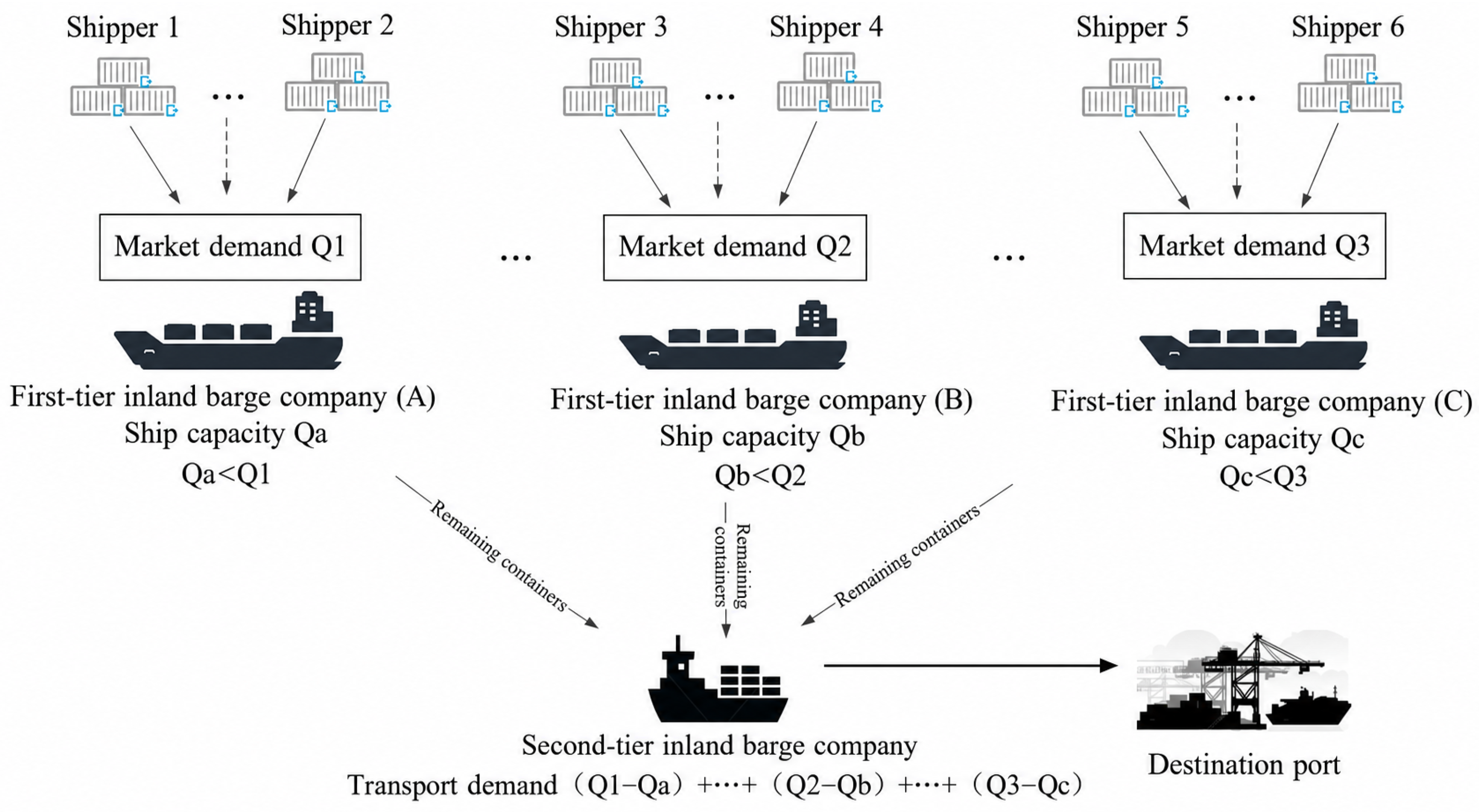
For the basis of our model, we consider a secondary port supply chain comprising one FTC and one STC. Both the FTC and the STC operate along the same shipping route and have a relatively fixed shipping capacity that cannot change in the short term. They have signed a long-term shipping space agreement that includes the agreed volume. Only the FTC undertakes the container transportation demand of shippers into the inland waterway market. The finite shipping capacity of the FTC, however, means that the firm cannot satisfy inland barge market demand every time. When market demand exceeds the FTC’s shipping capacity, the excess cargo will be transported by the STC. Moreover, when the extra cargo exceeds the volume contracted by the STC, the FTC will purchase temporary shipping space at a higher price from other STCs in the leftover-cargo spot market. The model is shown in Figure 2. The leftover-cargo freight market can thus be divided into two categories, namely, the agreement leftover market and the spot leftover market. According to the theory of revenue management, the STC should adopt different pricing strategies for customers operating in different markets. In the agreement leftover market, the long-term collaboration between two firms should be considered in the formulation of pricing, and the goal is to seek a pricing structure that can produce a win–win result. In the spot leftover market, however, an STC does not need to consider the cooperative relationship when setting prices. The STC instead takes the maximization of the individual firm’s revenue as the goal, and formulates a price that can improve the marginal value of its available shipping space. To sum up, the revenue optimization process of the STC comprises two stages: the first stage is setting cooperative pricing in the agreement leftover market, which can be modeled with game theory. The second stage is to set temporary prices in the spot leftover market, and must use the dynamic pricing method based on customer classification. Our paper focuses primarily on the cooperative pricing in the agreement leftover market in the first stage. The above setting is modeled as a one-FTC/one-STC benchmark analytical structure in order to isolate the core pricing mechanism of the leftover-cargo mode. In practice, the market may also involve several FTCs competing for the same shipper demand. Such horizontal competition among FTCs is not incorporated into the present model, because it would introduce an additional pricing layer on top of the current FTC–STC interaction. If multiple FTCs were considered, stronger FTC-side competition would likely further restrict the feasible market price, compress FTC profit margins, and reduce the surplus that can be shared with STCs. The analysis of multi-FTC competition is therefore left as an important extension for future research.

3.1. Notation and Assumptions

3.1.1. Notation

The game models in this paper are formulated based on the following notations:
  • D ( r , ε ) : The random demand function of the leftover freight market
  • r: The market price that shippers pay to the FTC
  • ε : The random demand factor
  • r * : The market price ceiling, determined by the competition between barges and trucks
  • q: The agreed volume between the FTC and STC
  • p: The agreed price that the FTC pays to the STC
  • p : The spot price in the spot leftover market
  • c: The unit transportation cost to the STC
  • z: The agreed volume factor
  • π 1 j ( · ) : The expected profit function of the FTC under model j, j ϵ { S , F , N }
  • π 2 j ( · ) : The expected profit function of the STC under model j, j ϵ { S , F , N }
  • π j ( · ) : The expected profit function of the entire supply chain under model j, j ϵ { S , F , N , C }
  • ( · ) j : The equilibrium results under model j without r * , j ϵ { S , F , N , C }
  • ( · ) j * : The equilibrium results under model j with r * , j ϵ { S , F , N , C }

3.1.2. Basic Assumptions

As in many previous studies, we make two assumptions so as to facilitate the subsequent modeling and analysis. In addition, the benchmark model focuses on the short-run pricing decision in the agreement leftover market. The parameter c represents the STC’s marginal unit transportation cost for carrying the agreed leftover containers. The FTC’s own vessel operating cost is not explicitly modeled because its planned sailing capacity and corresponding fixed operating cost are treated as predetermined in this short-run setting. Therefore, the FTC’s marginal decision concerns the market price, the agreed volume, and the payment to the STC. This simplification helps isolate the pricing interaction between the FTC and STC, while long-run cost heterogeneity, scale economies, and fleet-deployment decisions can be incorporated in future extensions by introducing separate cost parameters for FTCs and STCs.
Assumption 1. 
Suppose that ε is a random variable with a mean value of zero, and is differentiable in order to facilitate the analysis. Then, its distribution function F ( · ) and density function f ( · ) satisfy the following function: f ( x ) > f 2 ( x ) / F ( x ) . Similar assumptions have been made in earlier pricing models [62,67].
Assumption 2. 
In order to reach and maintain a long-term, cooperative relationship, the agreed price must be lower than the price in the spot leftover market, that is, p < p .

3.2. Demand Function and Profit Function

The demand function is generally composed of both expected demand and random fluctuations [68]. Expected demand is related to the market price, and is denoted as y ( r ) . Random fluctuations represent the uncertainty of market demand, and are denoted by ε . Common market demand functions include the linear price function y ( r ) = a b r ( a > 0 , b > 0 ) , the exponential price function y ( r ) = a e b r ( a > 0 , b > 0 ) , the fixed elasticity coefficient price function y ( r ) = a r b ( a > 0 , b > 1 ) , and so on. There are two forms of random demand fluctuation: additive demand and multiplicative demand fluctuations. For products with a relatively stable market demand, the additive demand function should be used. While for products with a market demand that responds more readily to price changes, the multiplicative demand function should be used. Accordingly, the linear additive demand specification used in this paper should be understood as a benchmark demand setting for a relatively stable agreement leftover market, rather than as a universal demand form. Exponential demand, fixed-elasticity demand, and multiplicative demand fluctuations may be more suitable when demand is highly elastic or when price changes alter the relative magnitude of demand uncertainty. These alternative demand specifications would change the analytical form of the equilibrium conditions and are therefore left for future robustness analysis rather than incorporated into the present closed-form benchmark model. As the cooperation between the FTC and STC in the agreement leftover market is based on relatively stable market demand, this paper assumes that the expected demand for leftover freight transportation is a linear function of market prices, and that any fluctuations are additive. That is, the random demand function can be expressed as:
D ( r , ε ) = y ( r ) + ε = a b r + ε , ( a > 0 , b > 0 )
In this formulation, the amount of cargo available in the market is represented through the demand function D ( r , ε ) = a b r + ε , where a captures the average market demand level and ε captures random demand fluctuations. Therefore, cargo availability affects the equilibrium results through market demand, agreed volume, and profit realization.
The FTC purchases the agreed freight space from the STC at the agreed price. For the leftover market demand that exceeds this agreed-upon volume, the FTC will purchase temporary additional space from the spot leftover market at the spot price. Then, the profit function of the FTC should be described as:
π 1 ( r , q ) = r D ( r , ε ) p q , D ( r , ε ) q r D ( r , ε ) p q p D ( r , ε ) q , D ( r , ε ) > q
We can derive a convenient expression for Equation (2) by substituting D ( r , ε ) = a b r + ε . Consistent with [68], we define an agreed volume factor z, as: z = q a + b r . Then:
π 1 ( r , z ) = r ( a b r + ε ) p ( a b r + z ) , ε z r ( a b r + ε ) p ( a b r + z ) p ( ε z ) , ε > z
As a result, we can obtain another explanation for shipping space decisions. If the decision value of z is greater than the realized value of ε , then there is a surplus of shipping space; otherwise, a shortage of shipping space occurs. Then, the FTC’s expected profit function under the three, distinct, decentralized game models (found in the subsequent section) can be expressed as:
π 1 j ( r , z ) = z r ( a b r + x ) p ( a b r + z ) f ( x ) d x + z + r ( a b r + x ) p ( a b r + z ) p ( x z ) f ( x ) d x = ( r p ) ( a b r ) p z p z [ 1 F ( x ) ] d x , j { S , F , N }
Random fluctuations in demand are not relevant to the STC’s expected profit:
π 2 j ( p ) = ( p c ) q j { S , F , N } s . t . c < p < p
Similarly, we can describe the expected profit of the supply chain under the centralized game model (details in the subsequent section):
π C ( r , z ) = ( r c ) ( a b r ) c z p z [ 1 F ( x ) ] d x

3.3. Game Models

In this section, we describe the equilibrium results of four game models, including three decentralized and one centralized game theory model. In the decentralized models, both companies maximize their own profits through independent decision-making, while in a centralized model, they aim to maximize the profits of the whole supply chain. The decision sequence is defined as a two-stage game. In the pricing stage, firms choose the relevant prices; after these prices are observed, the FTC chooses the agreed volume q, equivalently z = q a + b r . In model S, the STC first sets p, and the FTC then chooses r and z. In model F, the FTC first announces r, the STC then sets p, and the FTC finally chooses z. In model N, the FTC and STC simultaneously choose r and p, respectively, and the FTC then chooses z as its booking response. In model C, a centralized decision maker jointly chooses r and z. Thus, all decentralized models follow the sequence of pricing first and booking quantity later, and the Stackelberg models are solved by backward induction. The Appendix A gives detailed proofs for the propositions described in the following sections.

3.3.1. The STC-Stackelberg Model (Model S)

Under this model, the STC is regarded as the Stackelberg leader who chooses the agreed price p, while the FTC is the follower, responding by simultaneously determining the market price r and the agreed volume q. When solving the Stackelberg game theory model, the backward induction method is used. That is, we first determine the optimal agreed volume q and the market price r necessary for the FTC to maximize its expected profit under a given agreed price p. Then, we solve for the optimal agreed price p that maximizes the STC’s expected profit according to q and r. The model can be formulated as max r , z π 1 S ( r , z ) and max p π 2 S ( p ) , and Proposition 1 can be derived from Equations (5) and (6).
Proposition 1. 
Under model S, the agreed price p S , the market price r S , and the agreed volume q S at equilibrium are, respectively:
p S = p p F ( z S )
r S = a + b p b p F ( z S ) 2 b
q S = a b p + b p F ( z S ) 2 + z S
Proposition 1 shows the optimal pricing and the agreed volume decisions of both the FTC and STC in model S. We can conclude that the bigger the agreed volume factor z S , the bigger the agreed volume q S , and the lower the market price r S and the agreed price p S will be. Furthermore, the higher the spot price p , the higher the market price r S and the agreed price p S will be. We can derive that the demand D will decrease when the spot price p increases, which means that the competitiveness of inland barges decreases as the spot price rises.

3.3.2. The FTC-Stackelberg Model (Model F)

Under this model, the FTC is regarded as the Stackelberg leader while the STC is the follower. The FTC decides the market price r, and then the STC determines the agreed price p in line with the FTC’s decision. Finally, the FTC determines the agreed volume q.
Similarly, we use backward induction to solve model F and derive Proposition 2.
Proposition 2. 
Under model F, the market price r F , the agreed price p F , and the agreed volume q F at equilibrium are, respectively:
r F = 1 b [ c p p f ( z F ) + a + z F + F ( z F ) f ( z F ) ]
p F = p p F ( z F )
q F = p c p f ( z F ) F ( z F ) f ( z F )
Similar to Proposition 1, the bigger the agreed volume factor z F , the lower the market price r F and the agreed price p F will be under model F. The relationships between the market price r F and the agreed volume q F are more complicated than those in model S, because the density function of demand fluctuations f ( · ) is present here.

3.3.3. The Nash Model (Model N)

In this model, the FTC and STC hold equal pricing leadership, so that they each simultaneously make decisions regarding the market price r and the agreed price p in order to maximize their own expected profits while taking the other firm’s decisions into consideration. Then, the FTC determines the agreed volume q.
In the same way, we can obtain the equilibrium outcomes and derive Proposition 3.
Proposition 3. 
Under model N, the agreed price p N , the market price r N , and the agreed volume q N at equilibrium are, respectively:
p N = p p F ( z N )
r N = a + b p b p F ( z N ) 2 b
q N = a b p + b p F ( z N ) 2 + z N
From Proposition 3, we can derive that all the equilibrium decisions under model N have the same form as those in model S. In particular, the function expressions of the equilibrium agreed price in each of the three decentralized scenarios are the same.

3.3.4. The Centralized Model (Model C)

In this case, the decision-making does not have a priority relationship, as the market price r and the agreed volume q are decided in a coordinated manner, with the goal of maximizing the supply chain’s expected profit. In this model, it appears that the FTC and STC both belong to one firm, and that just one decision maker selects the market price r and the agreed volume q, thereby maximizing the total expected profit.
From Equation (6), we can derive Proposition 4 using backward induction.
Proposition 4. 
Under model C, the market price ( r C ), the agreed volume factor ( z C ), and the agreed volume ( q C ) at equilibrium are, respectively:
r C = a + b c 2 b
z C = F 1 ( p c p )
q C = a b c 2 + z C
Proposition 4 points out that the market price r C is only concerned with the unit transportation cost c, while the agreed volume q C is also influenced by the price in the spot leftover market p . We can thus conclude from Propositions 1–4 that the price and volume decisions at equilibrium depend on p as well as on the channel leadership.

4. Result Discussion

In this section, we make a comparative analysis of the agreed price, the market price, the agreed volume factor, the agreed volume, and the expected profits of each company and the supply chain at equilibrium under different models. Before comparing the equilibria, we clarify the mathematical basis of the comparison. Under Assumption 1 and c < p < p , the first-order conditions define equilibrium candidates within the feasible region. The Hessian or second-order conditions reported in the Appendix A verify the local optimality of these candidates, and the monotonicity conditions implied by Assumption 1 are used to establish the uniqueness of the corresponding agreed-volume factors. The following propositions summarize the economic ordering implied by these equilibrium candidates.
Proposition 5. 
p N p F p S and z N z F z S z C .
Proposition 5 implies that the dominant position of any barge company will lead to a decline in the agreed price and that the agreed price is always lower when the STC has more power. Interestingly, the agreed volume factor and the agreed price are inversely proportional. Further, the agreed volume factor in the centralized game model is greater than that in any of the decentralized models.
Proposition 6. 
r C r S r N r F .
Proposition 6 reveals that the market price decreases with a transfer of leadership from the FTC to the STC. Furthermore, a centralized supply chain achieves a lower market price compared with a decentralized supply chain. From Equation (1), we know that as the market price decreases, the leftover freight market demand increases. Thus, Proposition 6 has great significance in revealing how channel leadership influences the market competitiveness of inland waterway transportation. This result also confirms the superiority of centralized supply chains for lowering prices and improving the market position of barge transportation.
Proposition 7. 
q F q N q S q C .
From Proposition 7, we know that as leadership shifts from the FTC to the STC, the agreed volume increases. Further, the centralized supply chain always leads to the maximum agreed volume. This leads us to the following observation: If a given STC aims to open the market and obtain more agreed volume in the early stages of operation, a centralized supply chain is the best choice for the company. More generally, the STC should aim to gain more power within a decentralized supply chain.
Proposition 8. 
(i) π 2 F π 2 N π 2 S , and (ii) π 1 F π 1 N , π 1 S π 1 N .
Proposition 8 compares the expected profits of each member in the supply chain under decentralized scenarios. The results show that channel leadership is a beneficial factor that helps the STC increase its profit. The FTC’s profit as a function of its leadership is U-shaped, which means the dominant position of any barge company in the supply chain will raise the FTC’s profit. However, it is fairly complicated to predict the relationship of the FTC’s equilibrium profits under two Stackelberg models. Our computational study indicates that both π 1 F π 1 S and π 1 F < π 1 S can occur.
Proposition 9. 
π F π N π S π C .
Proposition 9 compares the expected profits of the supply chain under each of the four game theory models. The result shows that a centralized supply chain produces greater profit than the decentralized ones, which also bolsters its high effectiveness. Further, the overall profit also increases as the STC’s power increases within the three decentralized supply chains.
We can deduce from Propositions 5–9 that the centralized supply chain is the optimal solution for the pricing problem at the heart of this research, because it decreases the cost to shippers, increases the profits of inland barge companies, and expands the inland waterway transportation market. Unfortunately, it is difficult to achieve effective centralization and integration for a supply chain consisting of more than one company, at which time model S becomes a better solution. That is, under most conditions, the STC should seek to gain more power and greater dominance within the supply chain.
Proposition 10. 
If r * r j , j { S , F , N , C } , all the equilibrium decisions are the same under the models with or without r * . If r * < r j , j { S , F , N , C } : (i) p j * = p j , j { S , N } , p F * > p F ; (ii) q j * > q j , j { S , F , N , C } ; (iii) π 1 j * < π 1 j , j { S , F , N } , π 2 J * > π 2 J , j { S , F , N } , π C * > π C .
Proposition 10 compares the optimal decisions and revenues of barge companies, both with and without the market price ceiling constraint. The result shows that the agreed price, the agreed volume, and the profits of the two companies at equilibrium may change only when the market price ceiling is smaller than r j . If r * < r j , then the agreed volumes under all models will increase, and the agreed price will increase only under model F. As for expected profits, the FTC’s profits will decrease, while the STC’s profits will increase under all models. From this, it is clear that a low market price ceiling is beneficial to the STC, so these firms should pay attention to the competitive situation of other barge and truck transportation, and attempt to obtain more transportation market information. The supply chain’s profit is a quadratic function of the market price ceiling. Because the optimal market price is not obtained at the maximum value of the quadratic function in the decentralized scenarios, it is impossible to directly compare the relationship between the supply chain’s profits with and without the r * constraint. This lack of comparability is because the relationship is related to the difference between the price value corresponding to the maximum value of the quadratic function and the optimal market price. On the other hand, it is clear that the supply chain’s profit is reduced in the centralized scenario if r * < r j .

5. Case Study

In this section, we provide an example based on real data to illustrate the equilibrium decisions and profits of supply chain participants under different scenarios (models). The benchmark parameter values reported in Table 1 were calibrated on the basis of field investigation of inland barge operations on the Foshan Shunde Port–Shenzhen Shekou Port route. Specifically, the field investigation combined interviews with enterprise managers and real operational data provided by the participating enterprise, and provided route-level information on leftover freight demand, transportation cost, spot-market conditions, and truck freight rates, from which the numerical inputs of the case study were specified. The observation period covered data collected during 2023 and 2024. We analyze the influences of channel leadership on the optimal results, as well as the most lucrative leadership scenario for each member. Additionally, we analyze the impact of the agreed price and the market price ceiling on overall supply chain performance. This case study illustrates the practical application of the model in the Pearl River Delta leftover-cargo setting. All numerical results and Figure 3, Figure 4, Figure 5, Figure 6, Figure 7, Figure 8 and Figure 9 were generated by the authors using MATLAB R2016b (MathWorks, Natick, MA, USA).

5.1. Analysis of the Optimal Values

In our case study, the STC is mainly engaged in the container transportation business between Foshan Shunde Port and the surrounding secondary port areas on the route to Shenzhen Shekou Port. The FTC also operates the route between Shunde and Shekou Ports with a relatively stable market volume. We obtained real data as the model parameter values for this case study through field investigation, as shown in Table 1. The leftover freight market demand generally presents a linear distribution, with an average of 50 TEU, a price elasticity of 0.012, and fluctuations within 10 TEU. The leftover market price ceiling r * is set as the average truck freight rate over the same distance, that is, 2100 RMB. This value is used as a benchmark ceiling because truck service is the most direct substitute for the same shipper demand.
Assuming that the random fluctuations in market demand ε are uniformly distributed between [−10, 10], the optimal results under each of the different game theory models are shown in Table 2 and Table 3.
It can be seen from Table 2 and Table 3 that the agreed price of 1358.9 RMB under model S is 2.9% lower than the 1399.3 RMB under model F, and 11.0% lower than the 1527.2 RMB under model N. Meanwhile, the profits of the STC have increased by 41.5% and 5.2% across model F and model N, respectively. These findings are consistent with Propositions 5 and 9 in the previous analysis, and also reveal that a lower agreed price does not mean lower profit for the STC. Proposition 6 compares the market price under different game theory models, which is also illustrated in Table 2. For decentralized scenarios, it is obvious that the market price is the lowest under model S and the highest under model F. As a result, model S not only increases the profit of the STC, but also decreases the cost of the shippers.
The existing literature reveals that if a decision maker obtains greater leadership in the channel, that actor will achieve higher profit [29]. We, however, gain somewhat different results when discussing the problem from the perspective of the FTC in this paper. Table 3 shows that the FTC’s profit is highest under model S: π 1 S is 10.5% higher than π 1 N , and 8.2% higher than π 1 F . This is because model S enables the STC to strive for a lower agreed price, which urges the FTC to reduce the market price, and finally expands the leftover market demand and improves the total income. In summary, the STC-Stackelberg scenario is best for both the FTC and the STC, and it maximizes social welfare. The government should therefore encourage and support STCs in gaining more pricing power through measures such as capital subsidies and financially favorable policies for STCs that help to establish enterprise alliances and integrate resources.
Furthermore, we contrast the market prices and the supply chain’s profits between the decentralized and centralized scenarios. As Table 3 shows, r C is 13.7% lower than r S , 16.3% lower than r N , and 22.4% lower than r F ; thus, the market price of model C is much smaller than that in any decentralized model. As for the supply chain’s profits, the circumstance is just the opposite. The supply chain realizes the largest profits under model C (followed by models S and N), and obtains the lowest under model F. π C is 16.2% higher than π S , 26.4% higher than π N , and 36.2% higher than π F . Therefore, the centralized model is more conducive to improvements in overall supply chain performance and the market competitiveness of barge transportation.
It can be seen from the above description that there is a ceiling to the adjustment of the market price. In order to investigate how this ceiling influences the decisions of both barge companies and supply chain performance, we compile Table 4 and Table 5 to show the equilibrium results under different models with r * . The market price ceiling is 2100 RMB, which is lower than any equilibrium market price under the four game theory models.
When considering the market price ceiling constraint r * , the agreed price under model F is not only higher than the value under model S, but even exceeds the value under model N. The profit of the FTC under model F, however, is much smaller than under either of the other two dominant models. This is because the higher agreed price leads to an increase in the transportation cost of leftover containers, while the market price ceiling greatly reduces the profit margin of the FTC. In particular, under the same dominant mode, if r * < r j , (i) the STC’s profit increases and the FTC’s profit decreases; (ii) the profits of the whole supply chain under models S, N, and C increase. This indicates that the growth in the STC’s profit exceeds the decline in the FTC’s profit. The exception is the profit of the supply chain under model F, which decreases. When barges and trucks are in fierce competition, some FTCs will be transformed into STCs due to the decline in profits. The government should thus closely monitor the competitive situation between these transportation modes in order to avoid too many FTCs transforming into STCs and breaking the balance of the leftover-cargo market. If necessary, additional policy support should be granted in order to ensure the profits of the FTCs in the market.

5.2. Analysis of the Agreed Price

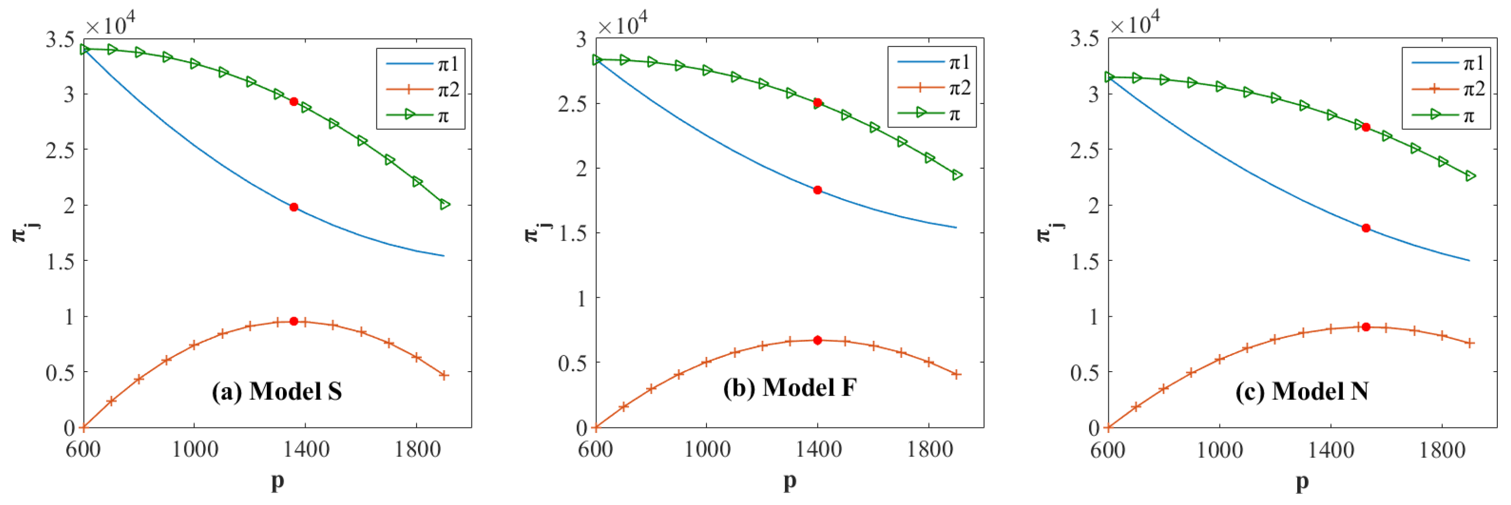
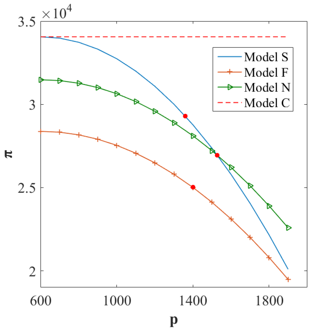
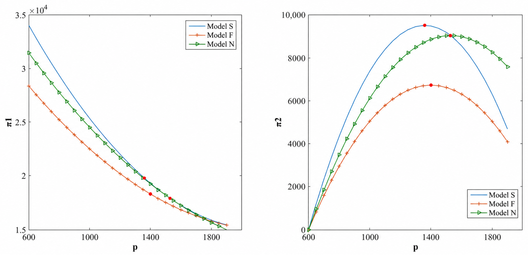
The agreed price p is an important factor that determines how much profit the STC can expect, and how much cost the FTC should allow for, which expectations in turn have great influence on the transaction between the two barge companies. In this section, we discuss the impact of the agreed price p on the equilibrium decisions and profits of the two companies, based on the parameters developed in Section 5.1. Figure 3, Figure 4 and Figure 5 demonstrate the equilibrium decisions and profits of each company under the FTC-Stackelberg model, the STC-Stackelberg model, the Nash model, and the centralized model. Figure 3 is drawn according to the pricing models, and it compares the profits of different aspects (FTC, STC, and SC) of the same model. Because the centralized model only considers the supply chain’s profit, Figure 3 only includes the three decentralized models. Figure 4 compares the profits of the FTC and the STC under each of the three decentralized pricing models, while Figure 5 compares the supply chain’s profits under the three decentralized models and the one centralized model.
Figure 3 shows that, as the agreed price p increases, the equilibrium profits of the FTC π 1 j and the supply chain π j decline, and π 1 j is convex while π j is concave with respect to p. As for the STC, profits first increase and then decrease with p, and the optimal solution is obtained at the highest point of the curve. The red markers in the graph reflect the equilibrium results with different channel leadership.
We should also note that a lower agreed price indicates that the FTC can afford a lower cost and is more willing to attempt to decrease the market price. The decrease in the market price increases the market demand and agreed volume sharply, which improves the overall competitiveness of barge companies on the market. Accordingly, the profits of the FTC and STC both increase. As shown in Figure 4, among the three decentralized models, the optimal agreed price is lowest in model S, followed by model F, while it is highest in model N. Thus, the highest profits for the two barge companies is in model S, followed by model F, and then by model N. These results are consistent with Propositions 5 and 8, confirming that model S is the best scenario for both parties.
Furthermore, we compare the centralized and decentralized scenarios. In the centralized game theory model, the two companies select the market price and the agreed volume with the goal of maximizing the supply chain’s expected profit, so π C is not concerned with the agreed price and is graphed as a straight line in Figure 5. Figure 5 clearly illustrates that π C is greater than the optimal expected profit projected by any of the decentralized game theory models. Therefore, model C is the optimum choice for the inland barge supply chain on the whole. As we mentioned before, however, it is difficult to achieve centralization and integration for a supply chain consisting of more than one company. Thus, given these realities, model S remains the next best solution.
In addition, the following leftover freight, transportation supply chain management insights are obtained from the above analysis: (i) These findings lead to a counterintuitive conclusion, namely, that it is not true that the higher the agreed price, the greater the profit of the STC. Due to the fact that an excessively high agreed price usually means an excessively high market price, the market demand and the agreed volume will decline sharply—an outcome that is not conducive to the development of the barge transportation market. This implies the importance of a proper pricing strategy carefully applied in order to increase a company’s profit. Further, the STC cannot consider only the individual costs of its own firm while making pricing decisions. An STC should rewrite its profit function in combination with the response of the FTC and the shipper to the agreed price in order to seek pricing equilibrium. (ii) Channel leadership greatly affects the pricing strategy of companies. Specifically, the case study shows that the STC-Stackelberg is a more effective strategy for developing a pricing strategy if a centralized supply chain is too difficult to achieve. At the initial stages in the development of the leftover-cargo mode, the overall status of STCs is relatively low, and the government should provide proper policy incentives and support so as to help STCs strive for pricing power that can be wielded to improve the total social welfare.

5.3. Analysis of the Market Price Ceiling

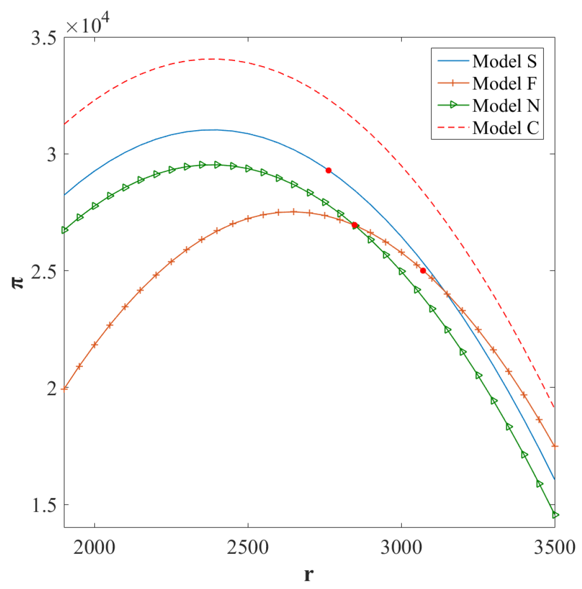
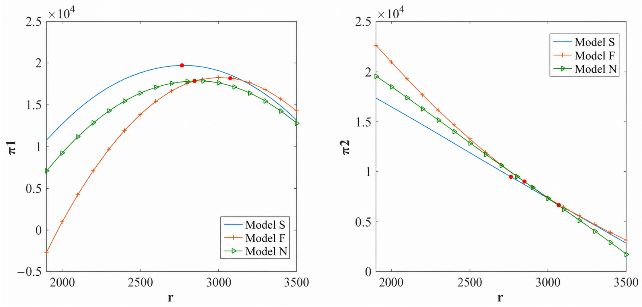
The market price ceiling determines the degree to which the FTC can raise the market price, which has a great impact on the pricing strategies of the two barge companies. In this section, we investigate the impact of the market price ceiling on the equilibrium results based on the parameters developed in Section 5.1. Before studying the influence of r * , we first need to clarify the relationship between the market price and the optimal solutions of the models, as shown in Figure 6, Figure 7, Figure 8 and Figure 9.
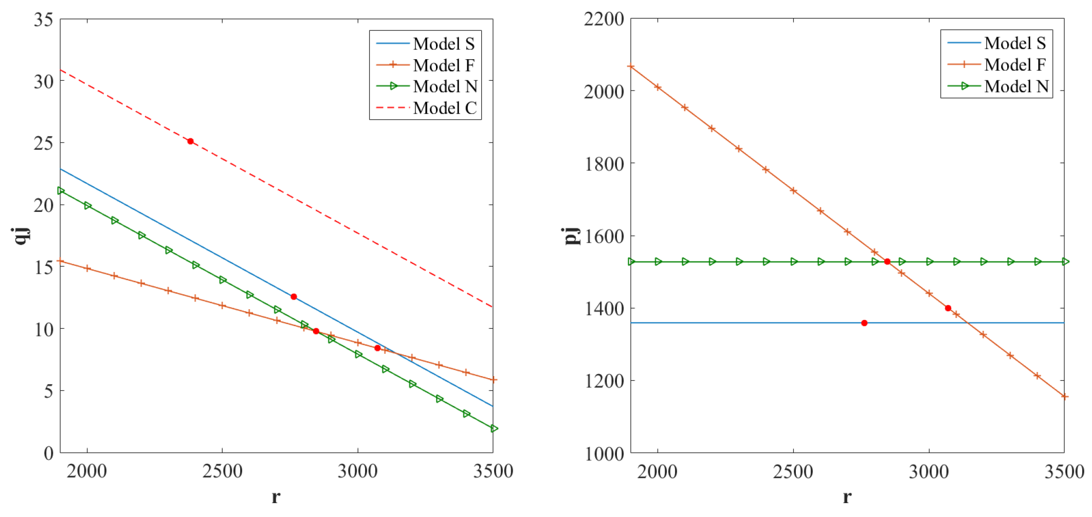
Figure 6 shows how the market price affects the optimal agreed volumes and the optimal agreed prices. As r increases, the agreed volumes under each of the four models decrease. The most significant reason for this is that, regardless of the channel leadership, a higher r increases the possibility of the FTC raising the market price, which in turn decreases market demand and the agreed volume. It is also clearly illustrated that q C is greater than the optimal agreed volume of any decentralized game theory model, which indicates that the centralized supply chain is beneficial to the STC in expanding the leftover freight market. As for the agreed price, only model F is affected, because under this model, the agreed price is determined through a pricing sequence driven by channel leadership. As r increases, the agreed price under model F decreases. In models S and N, on the other hand, the FTC determines the market price after the STC decides on the agreed price, so the agreed prices in those models are not affected by the change in market prices.
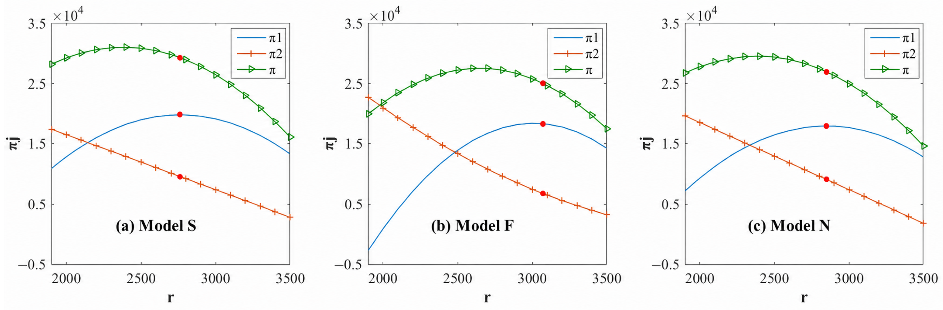
Figure 7, Figure 8 and Figure 9 show how the market price affects optimal profits. Figure 7 is drawn according to the pricing models. It compares the profits of different aspects of the same model. Because the centralized model only considers the supply chain’s profit, Figure 7 only includes the three decentralized models. Figure 8 compares the profits of the FTC and STC under each of the three decentralized pricing models, while Figure 9 compares the profit of the supply chain under the three decentralized models and the one centralized model.
Figure 7 implies that the optimal profit of the STC decreases with r, since both the agreed price and the agreed volume decrease with r. As for the FTC, its profit first increases and then decreases with r, as does the profit of the supply chain. It can be seen that barge companies cannot raise the market price indefinitely in order to increase their profits, because a higher market price leads to less market demand. As the red markers in the graph show, the optimal solution is obtained at the highest point of the FTC’s profit function, regardless of channel leadership. This is not, however, the optimal solution for the entire supply chain.
Figure 8 compares the equilibrium profits of the two barge companies under each of the decentralized scenarios. Each company’s equilibrium expected profits are the highest under model S. Meanwhile, we can compare the value of the optimal market price under the decentralized scenarios displayed in Figure 8: The optimal market price is lowest in model S, followed by model N, and then by model F. These results reveal that model S is the best option among the three decentralized scenarios.
Finally, Figure 9 compares the centralized and decentralized scenarios. On the whole (whether from the perspective of a low market price or high profits), the centralized supply chain has a significant advantage. If the supply chain is composed of two or more barge companies that cannot be readily integrated, however, the STC-Stackelberg model remains the best alternative.
It is worth noting that the optimal market price r j is obtained without considering the market price ceiling r * , and that the relationship between r j and r * will influence the pricing strategies of the barge companies. If r * r j , they will make a sensible decision according to r j of the game model, which is the x-value corresponding to the red point in Figure 8. If r * < r j , then the optimal pricing strategy for inland barge companies is to set prices in line with r * instead. At this time, π 1 is always highest under model S while π 2 is always highest under model F; however, which model provides the lowest result is uncertain. Therefore, we conclude the following: (i) The fierce competition between barges and trucks will provide more small and micro barge enterprises the option of entering the second-tier, which will in turn promote the development of the leftover-cargo mode and further improve the competitiveness of barge transportation. (ii) A barge company operating within the leftover-cargo mode should try its best to let the other take the lead if the market price ceiling is smaller than any equilibrium market price under a decentralized scenario. The channel leadership decisions (which game theory model among the three decentralized models is the best) differ from those in models that do not consider r * , which reveals the impact of r * on pricing strategies and the choices of channel leadership for barge companies. (iii) The centralized supply chain demonstrates both superiority and stability, because it can generate maximum profits regardless of the market price ceiling. As Figure 9 shows, the supply chain’s optimal profit in model C is still higher than that in any of the decentralized models.

6. Conclusions

While container transportation brings huge economic benefits, it inevitably causes the problem of congestion in the urban road network, noise, air pollution, and so on. Inland waterway transportation (as a more environmentally friendly hinterland transportation mode) lacks market competitiveness because its market responsiveness is not as good as that of truck transportation. The leftover-cargo mode provides the possibility of improving the overall competitiveness of inland navigation and achieving sustainable development: it reduces the market risk by integrating large and small enterprises, and enables barge companies to meet the needs of shippers with lower costs and higher responsiveness. Therefore, the government should encourage the implementation of the leftover-cargo mode so as to optimize the structure of inland waterway transportation and contribute to achieving carbon neutrality. This cooperation mode can also be referred to by other industries seeking to reduce risks caused by uncertain demand and improve the responsiveness and competitiveness of the industry.
Our paper finds that a centralized supply chain can maximize the overall performance of firms within this mode, producing superior profits and stability. It is fairly difficult, however, for enterprises to fully realize information sharing and interconnection. In a decentralized supply chain, the STC-Stackelberg pricing strategy can achieve both lower agreed and market prices, which not only improve the profits of the FTC and STC alike, but also reduce the transportation costs of shippers. Consequently, in the process of implementing the leftover-cargo mode, the government should provide support to STCs in order to help them obtain channel leadership and thus to optimize the revenue of inland waterway transportation.
The market price ceiling impacts the pricing of inland barge companies, as well. If the market price ceiling is lower than the equilibrium market prices given in the models, then more FTCs are likely to transform into STCs. Whether FTC or STC, they are willing to become a follower in a decentralized supply chain. But from the perspective of the entire supply chain, model S is the best alternative. The channel leadership decisions of the implicated enterprises will also be affected by the level of competition between barges and trucks. The government should thus treat this factor as an important basis for industrial policy-making. If r * < r j , the government should encourage STCs to acquire more pricing power and provide financial support to FTCs experiencing reduced profits so as to avoid a large number of FTCs transforming into STCs. The ultimate aim of these policy efforts would be to maintain the healthy and balanced development of the leftover-cargo mode, resulting in greater emissions reduction benefits.
Our paper provides new insights into channel leadership decisions and pricing strategies for inland barge companies under the leftover-cargo mode. These insights are derived from the analytical results of the model and illustrated through the case study. Nevertheless, research into the leftover-cargo supply chain is just beginning. The revenue management of the STC is a two-stage pricing model that responds to different markets. This paper only discusses the pricing problem of the contract market within the leftover-cargo mode. It remains a challenge to discuss the pricing problems in the spot market, which should be addressed in future research. Another boundary case may occur when the FTC can absorb all shipper demand during a certain period. In that case, the agreement leftover market becomes inactive, and the STC may receive little or no agreed-volume revenue while still maintaining vessels and crews for possible cooperation. The present paper does not model the STC’s survival horizon under such prolonged low-cargo periods, because this would require a dynamic framework with explicit standby-cost considerations. Future research may therefore examine the sustainability of STC participation under insufficient leftover cargo. Moreover, the models only analyze the linear additive demand function. For future research, we recommend analyzing pricing strategies with different types of stochastic demand functions.

Author Contributions

W.C., conceptualization, methodology, formal analysis, investigation; W.W., software, formal analysis, visualization, and writing—original draft preparation; Y.L., investigation, data curation, validation, and visualization; Y.G., conceptualization, methodology, supervision, project administration, and writing—review and editing; H.S.L., validation, supervision, and writing—review and editing. All authors have read and agreed to the published version of the manuscript.

Funding

This research received funding support from the Natural Science Foundation of Guangdong Province, China (Grant No. 2023A1515010950), and the Fundamental Research Funds for the Central Universities (grant number CXTD202407).

Institutional Review Board Statement

Ethical approval is not applicable for this article.

Informed Consent Statement

Not applicable.

Data Availability Statement

Data is contained within the article. The original contributions presented in this study are included in the article. Further inquiries can be directed to the corresponding author.

Conflicts of Interest

The authors declare no conflicts of interest.

Appendix A

Proof of Proposition 1. 
Using backward induction, first determine the optimal decisions for the FTC under a given agreed price. The objective is maximizing the FTC’s expected profit: max r , z π 1 ( r , z ) . Taking the first derivative of Equation (4) with respect to r and z, then setting them to 0, we obtain that:
π 1 r = a 2 b r + b p = 0
π 1 z = p + p [ 1 F ( z ) ] = 0
We can also obtain the Hessian matrix of π 1 as follows:
H ( r , z ) = 2 π 1 r 2 2 π 1 r z 2 π 1 z r 2 π 1 z 2 = 2 b 0 0 p f ( z )
Equation (A3) indicates that the Hessian matrix of π 1 is a negative definite for r and z. From Equations (A1) and (A2), we can derive that:
r ( p ) = a + b p 2 b
z ( p ) = F 1 ( p p p )
Recall that q ( p ) = a b r + z , we can obtain that:
q ( p ) = a b p 2 + z
Then, the STC predicts the market price and the agreed volume determined by the FTC based on Equations (A4)–(A6). Therefore, the problem in the first stage can be formulated as max p π 2 ( p ) . Substitute Equations (A5) and (A6) into Equation (5), then the expected profit of the STC is expressed as:
π 2 ( z ) = [ p p F ( z ) c ] [ a b p + b p F ( z ) 2 + z ]
Taking the first derivative of Equation (A7) with respect to z, then:
π 2 z = p f ( z ) [ a + 2 b p b c 2 b p F ( z ) z F ( z ) f ( z ) ] + p c
Define
T ( z ) = a + 2 b p b c 2 b p F ( z ) z F ( z ) f ( z )
Taking the first derivative of Equation (A9) with respect to z. We obtain that:
T ( z ) z = c p p · f ( z ) f ( z ) c p p · 1 F ( z ) = c p p p < 0
Because Equation (A10) is negative, thus π 2 z = 0 has the unique solution. Taking the second derivative of Equation (A7) with respect to z, we obtain that:
2 π 2 z 2 = p f ( z ) T ( z ) b p 2 f 2 ( z ) 2 p f ( z ) + p F ( z ) f ( z ) f ( z )
2 π 2 z 2 | z = z S = ( c p ) f ( z S ) f ( z S ) b p 2 f 2 ( z S ) 2 p f ( z S ) + ( p p ) f ( z S ) f ( z S ) = ( c p ) f ( z S ) f ( z S ) b p 2 f 2 ( z S ) 2 p f ( z S )
Recall that c < p < p ; we can find that:
2 π 2 z 2 | z = z S ( c p ) f ( z S ) F ( z S ) b p 2 f 2 ( z S ) 2 p f ( z S ) = [ c p p p 2 ] p f ( z S ) b p 2 f 2 ( z S ) < 0
Equation (A13) shows that π 2 ( z ) is concave to z. Then, we set Equation (A8) equal to 0, getting the optimal agreed volume factor z S in model S satisfies:
f ( z S ) T ( z S ) = c p p
Substituting Equation (A14) into Equation (A5), we obtain that the agreed price at equilibrium is
p S = p p F ( z S )
Substituting Equation (A15) into Equations (A4) and (A6), we can obtain that at equilibrium, the market price and the agreed volume are, respectively,
r S = a + b p b p F ( z S ) 2 b
q S = a b p + b p F ( z S ) 2 + z S
 □
Proof of Proposition 2. 
Using backward induction, first determine the optimal decisions for the FTC under the given market price and agreed price. It follows from Equations (A5) and (A6) that the agreed volume and the agreed volume factor determined by the FTC in model F satisfy
q = a b r + z ( p )
z ( p ) = F 1 ( p p p )
Then, the STC predicts that the agreed volume determined by the FTC according to Equations (A18) and (A19). Therefore, the problem in the second stage can be formulated as max z π 2 ( z ) . Substituting Equations (A18) and (A19) into Equation (5), then the expected profit of the STC is expressed as:
π 2 ( z ) = [ p p F ( z ) c ] ( a b r + z )
Taking the first derivative of Equation (A20) with respect to z, then:
π 1 z = p f ( z ) [ a + b r z F ( z ) f ( z ) ] + p c
Define
R ( z ) = c p p f ( z ) + a + z + F ( z ) f ( z )
Taking the first derivative of Equation (A22) with respect to z, we obtain that:
R ( z ) z = p c p · f ( z ) f ( z ) + 2 p c p p + 2 > 0
Note that Equation (A23) is positive; thus, π 2 z = 0 has the unique solution. Setting Equation (A21) equal to 0, the optimal agreed volume factor z F with given market price and agreed volume in model F satisfies:
R ( z F ) = b r F
Next, the problem in the first stage for the FTC can be formulated as max z π 1 ( z ) . Substituting Equations (A19) and (A24) into Equation (4), the expected profit of the FTC is expressed as:
π 1 ( z ) = [ R ( z ) b p + p F ( z ) ] [ a R ( z ) ] z p [ 1 F ( z ) ] p z [ 1 F ( z ) ] d x
The equilibrium agreed volume factor z F in model F must satisfy:
π 1 ( z ) z | z = z F = 0
Although our large computational studies have shown that it is quite complicated to establish the unimodality of π 1 F , we can apply an exhaustive search method to find out the equilibrium agreed volume factor z F . After solving Equation (A26) to get z F , we can obtain the market price, the agreed price, and the agreed volume at equilibrium:
r F = 1 b [ c p p f ( z F ) + a + z F + F ( z F ) f ( z F ) ]
p F = p p F ( z F )
q F = p c p f ( z F ) F ( z F ) f ( z F )
 □
Proof of Proposition 3. 
As is the case with the model F, with the market price and the agreed price known, the optimal decisions of the FTC in the last part follow from Equations (A18) and (A19):
q = a b r + z ( p )
z ( p ) = F 1 ( p p p )
Further analyze the optimal market price and the agreed price. Substituting Equations (A30) and (A31) into Equations (4) and (5), the expected profit of two companies are respectively
π 1 ( r , p ) = ( r p ) ( a b r ) p z p z [ 1 F ( x ) ] d x
π 2 ( r , z ) = [ p p F ( z ) c ] [ a b r + z ( p ) ]
Define
N ( z ) = a + b p b p F ( z ) 2 z F ( z ) f ( z )
Taking the first and the second derivative of Equation (A32) with respect to r, then:
π 1 ( r , p ) r = a + b p 2 b r
π 2 ( r , z ) = [ p p F ( z ) c ] [ a b r + z ( p ) ]
Thus, π 1 ( r , p ) is concave with respect to r for a given p. Taking the first and the second derivative of Equation (A33) with respect to z, then:
π 2 ( r , z ) z = p f ( z ) [ a + b r z F ( z ) f ( z ) ] + p c
2 π 2 ( r , z ) z 2 = p f ( z ) N ( z ) b p 2 f 2 ( z ) 2 p f ( z ) + p F ( z ) f ( z ) f ( z )
Thus, π 2 ( r , z ) is concave with respect to z for a given r. Therefore, setting Equations (A35) and (A37) equal to 0, we can obtain that the equilibrium agreed volume factor z N in model N satisfies:
f ( z N ) N ( z N ) = c p p
With z N obtained from Equation (A39), we can obtain all equilibrium outcomes as follows:
p N = p p F ( z N )
r N = a + b p b p F ( z N ) 2 b
q N = a b p + b p F ( z N ) 2 + z N
 □
Proof of Proposition 4. 
In model C, we solve the objective function of the supply chain’s expected profit.
Taking the first derivative of Equation (6) with respect to r and z. Then, setting them equal to 0, we obtain that:
π r = a + b p 2 b r = 0
π z = c p [ 1 F ( z ) ] = 0
We can also obtain the Hessian matrix of π as follows:
H ( r , z ) = 2 π 1 r 2 2 π 1 r z 2 π 1 z r 2 π 1 z 2 = 2 b 0 0 p f ( z )
Equation (A45) indicates that the Hessian matrix of π is a negative definite for r and z. Solving Equations (A43) and (A44), we can derive the equilibrium market price, the agreed volume factor:
r C = a + b c 2 b
z C = F 1 ( p c p )
Substituting Equations (A46) and (A47) into q ( p ) = a b r + z , we can obtain the agreed price at equilibrium as follows:
q C = a b c 2 + z C
 □
Proof of Proposition 5. 
Taking the first derivative of Equation (A25) with respect to z, we obtain that:
π 1 F z = R ( z ) b [ a 2 R ( z ) + b p ] p + p p F ( z ) = R ( z ) b { a 2 R ( z ) + b p [ 1 F ( z ) ] } = 2 R ( z ) b a + b p [ 1 F ( z ) ] 2 R ( z ) .
The second equality follows from p = p p F ( z ) = p [ 1 F ( z ) ] . According to Equations (A22) and (A34), we can obtain that:
R ( z ) N ( z ) = c p p f ( z ) + a + z + F ( z ) f ( z ) a + b p b p F ( z ) 2 z F ( z ) f ( z ) = c p p f ( z ) a a + b p [ 1 F ( z ) ] 2 = c p p f ( z ) a + b p [ 1 F ( z ) ] 2 .
Rearranging Equation (A50) gives
a + b p [ 1 F ( z ) ] 2 R ( z ) = N ( z ) c p p f ( z ) .
Substituting Equation (A51) into Equation (A49), we can obtain that:
π 1 F z = 2 R ( z ) b N ( z ) c p p f ( z ) .
We next verify the second-order condition used for model N. Since the reduced optimization problem of the STC with respect to z is one-dimensional, its Hessian matrix is
H N ( z ) = 2 π 2 N z 2 .
From Equation (A33), together with the definition of N ( z ) in Equation (A34),
π 2 N z = p f ( z ) N ( z ) + p c .
Therefore,
2 π 2 N z 2 = p f ( z ) N ( z ) + p f ( z ) N ( z ) = p f ( z ) N ( z ) b p 2 f 2 ( z ) 2 p f ( z ) + p F ( z ) f ( z ) f ( z ) .
Under Assumption 1 and the feasible price condition c < p < p , the leading principal minor of H N ( z ) is negative at the stationary point z N . By Sylvester’s criterion for a one-dimensional Hessian matrix, H N ( z N ) is negative definite. Hence, π 2 N is locally strictly concave at z N , and the stationary point satisfying
f ( z N ) N ( z N ) = c p p
is the unique interior maximizer in model N. Because Equation (A33) is concave, when z z N , we can obtain that:
π 2 N z = p f ( z ) N ( z ) + p c 0 .
Since p > 0 and f ( z ) > 0 , Equation (A57) is equivalent to
N ( z ) c p p f ( z ) .
Substituting Equation (A58) into Equation (A52), we can obtain that:
π 1 F z = 2 R ( z ) b N ( z ) c p p f ( z ) 0 , z z N .
Because R ( z ) > 0 from Equation (A23) and b > 0 , Equation (A59) shows that π 1 F ( z ) cannot attain an interior maximum at any point strictly smaller than z N . Therefore, any interior equilibrium solution z F of model F must satisfy
z N z F .
According to Equations (A9) and (A22), we can obtain that:
R ( z ) T ( z ) = c p p f ( z ) + a + z + F ( z ) f ( z ) a + 2 b p b c 2 b p F ( z ) z F ( z ) f ( z ) = c p p f ( z ) a a + 2 b p b c 2 + b p F ( z ) = c p p f ( z ) a b c + 2 b p [ 1 F ( z ) ] 2 .
Rearranging Equation (A61) yields
a + b p [ 1 F ( z ) ] 2 R ( z ) = T ( z ) c p p f ( z ) + b { c p [ 1 F ( z ) ] } 2 .
Because p = p [ 1 F ( z ) ] , Equation (A62) can be rewritten as
a + b p [ 1 F ( z ) ] 2 R ( z ) = T ( z ) c p p f ( z ) + b ( c p ) 2 .
Substituting Equation (A63) into Equation (A49), we can obtain that:
π 1 F z = 2 R ( z ) b T ( z ) c p p f ( z ) + b ( c p ) 2 .
Similarly, for model S, the reduced optimization problem of the STC with respect to z is one-dimensional, and its Hessian matrix is
H S ( z ) = 2 π 2 S z 2 .
From Equation (A7) and the definition of T ( z ) in Equation (A9),
π 2 S z = p f ( z ) T ( z ) + p c .
Thus,
2 π 2 S z 2 = p f ( z ) T ( z ) + p f ( z ) T ( z ) = p f ( z ) T ( z ) b p 2 f 2 ( z ) 2 p f ( z ) + p F ( z ) f ( z ) f ( z ) .
Under Assumption 1 and the feasible price condition c < p < p , the leading principal minor of H S ( z ) is negative at the stationary point z S . Hence, by Sylvester’s criterion, H S ( z S ) is negative definite. Therefore, π 2 S is locally strictly concave at z S , and the stationary point satisfying
f ( z S ) T ( z S ) = c p p
is the unique interior maximizer in model S. Because Equation (A7) is concave, when z z S , we can obtain that π 2 S z 0 . That is,
π 2 S z = p f ( z ) T ( z ) + p c 0 .
Accordingly, the relationship between Equation (A9) and f ( z ) is expressed as follows:
T ( z ) c p p f ( z ) .
Substituting Equation (A70) into Equation (A64), we can obtain that:
π 1 F z = 2 R ( z ) b T ( z ) c p p f ( z ) + b ( c p ) 2 0 , z z S .
The last inequality follows from c < p , R ( z ) > 0 , and b > 0 . Thus, π 1 F ( z ) cannot attain an interior maximum at any point strictly larger than z S . Combining Equations (A60) and (A71), any interior equilibrium solution of model F satisfies
z N z F z S .
Therefore, the comparison result is valid for any interior equilibrium solution of model F. If the maximizer of π 1 F ( z ) obtained from Equation (A26) is unique, then the equilibrium z F is unique; if several maximizers exist, every equilibrium maximizer still lies in the interval [ z N , z S ] . Because c p S , according to Equations (A15) and (A47), we can obtain that z S z C . Specifically, Equation (A15) gives F ( z S ) = ( p p S ) / p , while Equation (A47) gives F ( z C ) = ( p c ) / p . Since c p S ,
p p S p p c p .
Because F ( · ) is increasing, Equation (A73) implies z S z C . Hence,
z N z F z S z C .
From Propositions 1, 2, 3, and 5, we can know p j = p p F ( z j ) , j { S , F , N } and z N z F z S ; thus, p N p F p S . Indeed, since F ( · ) is increasing, z N z F z S implies F ( z N ) F ( z F ) F ( z S ) . Multiplying by p < 0 reverses the inequality, and adding p to all terms gives
p p F ( z N ) p p F ( z F ) p p F ( z S ) .
Therefore, p N p F p S .
  □
Proof of Proposition 6. 
We next verify the second-order conditions that support the uniqueness of the market price decisions used below. For models S and N, after the agreed price is given, the FTC’s expected profit with respect to r is obtained from Equation (4). The first and second derivatives with respect to r are
π 1 r = a + b p 2 b r ,
H r = 2 π 1 r 2 = 2 b .
Since b > 0 , the only leading principal minor of H r is 2 b < 0 . By Sylvester’s criterion for a one-dimensional Hessian matrix, H r is negative definite. Hence, π 1 is strictly concave in r, and the first-order condition π 1 r = 0 gives a unique market-price best response
r = a + b p 2 b .
For model C, the supply chain profit in Equation (6) has the Hessian matrix with respect to ( r , z )
H C ( r , z ) = 2 π C r 2 2 π C r z 2 π C z r 2 π C z 2 = 2 b 0 0 p f ( z ) .
Because b > 0 , p > 0 , and f ( z ) > 0 , its leading principal minors satisfy
Δ 1 = 2 b < 0 , Δ 2 = ( 2 b ) ( p f ( z ) ) = 2 b p f ( z ) > 0 .
Thus, H C ( r , z ) is negative definite by Sylvester’s criterion. Therefore, the centralized supply chain profit is strictly concave in ( r , z ) , and the centralized equilibrium market price r C is unique. For model F, once the equilibrium agreed volume factor z F is obtained from Equation (A26), Equation (A27) gives a unique corresponding market price r F = R ( z F ) / b . From Propositions 1, 3, 4, and 5, we have r S = a + b p S 2 b , r N = a + b p N 2 b , r C = a + b c 2 b and c p S p N , thus r C r S r N . The detailed derivation is as follows. First,
r S r C = a + b p S 2 b a + b c 2 b = b ( p S c ) 2 b = p S c 2 .
Since p S c , Equation (A81) implies r S r C 0 , and therefore r C r S . Similarly,
r N r S = a + b p N 2 b a + b p S 2 b = b ( p N p S ) 2 b = p N p S 2 .
Since Proposition 5 gives p N p S , Equation (A82) implies r N r S 0 , and therefore r S r N . Combining these two inequalities gives
r C r S r N .
Define ω ( z ) = R ( z ) b , then:
ω ( z ) | z = z N = 1 b c p p f ( z N ) + a + z N + F ( z N ) f ( z N ) .
Substituting Equation (A39) into Equation (A84), we can obtain that:
ω ( z ) | z = z N = 1 b N ( z N ) + a + z N + F ( z N ) f ( z N ) = 1 b a + b p b p F ( z N ) 2 z N F ( z N ) f ( z N ) + a + z N + F ( z N ) f ( z N ) = 1 b a + b p b p F ( z N ) + 2 a 2 = a + b p b p F ( z N ) 2 b = r N ( z ) | z = z N = r N .
The first equality in Equation (A85) follows from Equation (A39), namely
f ( z N ) N ( z N ) = c p p N ( z N ) = c p p f ( z N ) .
Taking the first derivative of ω ( z ) with respect to z, then:
d ω ( z ) d z = 1 b R ( z ) > 0 .
The inequality in Equation (A87) follows from b > 0 and R ( z ) > 0 in Equation (A23). Hence, ω ( z ) is strictly increasing in z. More explicitly, for any z 2 z 1 ,
ω ( z 2 ) ω ( z 1 ) = z 1 z 2 ω ( x ) d x = z 1 z 2 R ( x ) b d x 0 .
From Proposition 5, we can know z N z F , thus
r F = ω ( z ) | z = z F     ω ( z ) | z = z N = r N .
Combining Equation (A83) with Equation (A89), we obtain
r C r S r N r F .
The strict concavity results above also show that the market price solutions r S , r N , and r C exist and are unique. In model F, given the equilibrium agreed volume factor z F obtained from Equation (A26), the market price r F = R ( z F ) / b is uniquely determined. Therefore, the equilibrium comparison in Proposition 6 is well-defined. □
Proof of Proposition 7. 
From Propositions 1–4, we can know q j = a b r j + z j , j = { S , F , N , C } . From Propositions 5 and 6, we have z N z F z S z C and r C r S r N r F , thus q N q S q C and q F q S q C . More specifically, q S q N = ( a b r S + z S ) ( a b r N + z N ) = b ( r N r S ) + ( z S z N ) 0 , because r N r S and z S z N ; q C q S = ( a b r C + z C ) ( a b r S + z S ) = b ( r S r C ) + ( z C z S ) 0 , because r S r C and z C z S ; and q S q F = ( a b r S + z S ) ( a b r F + z F ) = b ( r F r S ) + ( z S z F ) 0 , because r F r S and z S z F . Therefore, q N q S q C and q F q S q C . Next, we prove q F q N . Define η ( z ) = p c p f ( z ) F ( z ) f ( z ) , then:
η ( z ) | z = z N = p c p f ( z N ) F ( z N ) f ( z N )
Substituting Equation (A39) into Equation (A91), we can obtain that:
η ( z ) | z = z N = c p p f ( z N ) F ( z N ) f ( z N ) = N ( z N ) F ( z N ) f ( z N ) = a + b p b p F ( z N ) 2 z N F ( z N ) f ( z N ) F ( z N ) f ( z N ) = a b p + b p F ( z N ) 2 + z N = q N ( z ) | z = z N = q N
Here, Equation (A39) is used in the form N ( z N ) = ( c p ) / [ p f ( z N ) ] . Taking the first derivative of η ( z ) with respect to z, then:
d η ( z ) d z = d d z p c p f ( z ) F ( z ) f ( z ) = p c p f ( z ) f 2 ( z ) f 2 ( z ) F ( z ) f ( z ) f 2 ( z ) = 1 + F ( z ) p c p f ( z ) f 2 ( z ) = 1 R ( z ) < 0
The equality d η ( z ) d z = 1 R ( z ) follows from differentiating Equation (A22); Equation (A23) gives R ( z ) > 1 , so η ( z ) is strictly decreasing in z. Because z N z F , thus
q F = η ( z ) | z = z F η ( z ) | z = z N = q N
Combining q F q N with q N q S q C , we obtain q F q N q S q C . The negative definiteness of the one-dimensional Hessian H q ( z ) also confirms the existence and uniqueness of the agreed volume decision given the equilibrium prices. Therefore, the equilibrium comparison in Proposition 7 is well-defined. □
Proof of Proposition 8. 
The existence and uniqueness of the equilibrium components used below follow from the second-order conditions in the preceding propositions. For the STC’s one-dimensional pricing problem in models S and N, the Hessian matrix is H 2 j ( z ) = 2 π 2 j / z 2 , j { S , N } . At the stationary points z S and z N , the leading principal minor is negative under Assumption 1 and c < p < p ; hence H 2 S ( z S ) and H 2 N ( z N ) are negative definite by Sylvester’s criterion. Thus, π 2 S and π 2 N are strictly concave at their respective stationary points, and z S and z N are unique interior maximizers. For the FTC’s last-stage agreed-volume decision, the Hessian is H q ( z ) = p f ( z ) , which is negative definite because p > 0 and f ( z ) > 0 . Hence, the agreed volume is uniquely determined once the equilibrium prices are given. In model F, after an equilibrium agreed volume factor z F is selected from Equation (A26), the corresponding p F , r F , and q F are uniquely determined by Equations (A27)–(A29). (i) The STC’s expected profit under three decentralized game models can be rewritten as:
π 2 j ( z j ) = [ p p F ( z j ) c ] a b p + b p F ( z j ) 2 + z j , j { S , N }
π 2 F ( z F ) = [ p p F ( z F ) c ] [ a R ( z F ) + z F ]
According to Equation (A50), we can obtain that:
π 2 F z F = [ p p F ( z F ) c ] N ( z F ) c p p f ( z F ) + a b p + b p F ( z F ) 2 + z F = [ p p F ( z F ) c ] N ( z F ) c p p f ( z F ) + [ p p F ( z F ) c ] a b p + b p F ( z F ) 2 + z F = [ p p F ( z F ) c ] N ( z F ) c p p f ( z F ) + π 2 N ( z F )
The first equality in Equation (A97) follows by rearranging Equation (A50). Specifically, Equation (A50) implies a + b p [ 1 F ( z ) ] 2 R ( z ) = N ( z ) c p p f ( z ) . Since a + b p [ 1 F ( z ) ] 2 = a + b p b p F ( z ) 2 , adding z to both sides gives a R ( z ) + z = N ( z ) c p p f ( z ) + a b p + b p F ( z ) 2 + z . This explains the decomposition in Equation (A97). From Proposition 5, z N z F . Since π 2 N ( z ) is concave and reaches its maximum at z N , it is nonincreasing for z z N . Therefore, π 2 N ( z F ) π 2 N ( z N ) = π 2 N . Moreover, the first-order condition of model N gives N ( z N ) = c p p f ( z N ) . For z z N , concavity implies π 2 N / z = p f ( z ) N ( z ) + p c 0 , which is equivalent to N ( z ) c p p f ( z ) because p > 0 and f ( z ) > 0 . Evaluating this inequality at z = z F gives N ( z F ) c p p f ( z F ) 0 . Since the feasible agreed price satisfies p F = p p F ( z F ) > c , the coefficient p p F ( z F ) c is positive. Hence, the first term on the right-hand side of Equation (A97) is nonpositive, and therefore π 2 F ( z F ) π 2 N ( z F ) π 2 N .Next, we compare model N with model S. For any common value of z, Equation (A95) shows that π 2 S ( z ) and π 2 N ( z ) have the same functional form. Therefore, π 2 S ( z N ) = π 2 N ( z N ) = π 2 N . Since z S is the unique maximizer of π 2 S ( z ) , we have π 2 S ( z S ) π 2 S ( z N ) . Thus, π 2 S π 2 N . Combining the two comparisons gives π 2 F π 2 N π 2 S . (ii) Rewrite the expected profit function of the FTC under three decentralized game models:
π 1 j ( r , z ) = [ r p + p F ( z j ) ] ( a b r ) z j [ c p F ( z j ) ] p z j [ 1 F ( x ) ] d x , j { S , F , N }
Substituting Equations (A19), (A28), (A31) and (A40) into Equation (A98), because p F ( z ) | z = z N = p N , we can obtain that:
π 1 F ( z ) | z = z N = π 1 N ( z ) | z = z N = π 1 N
Indeed, p F ( z ) = p p F ( z ) and p N = p p F ( z N ) , so evaluating p F ( z ) at z = z N gives p F ( z ) | z = z N = p N . At the same value z = z N , Equation (A24) gives r F ( z ) | z = z N = R ( z N ) / b , and the proof of Proposition 6 shows that R ( z N ) / b = r N . Therefore, the FTC profit under model F evaluated at z N coincides with the FTC profit under model N at its equilibrium. This justifies Equation (A99). Because π 1 F ( z ) | z = z F = max z π 1 F ( z ) , we have π 1 F z | z = z F     π 1 F z | z = z N , thus π 1 F π 1 N . This comparison only uses the optimality of z F in model F. If the maximizer of π 1 F ( z ) is unique, then the equilibrium profit π 1 F is unique. If multiple maximizers exist, every selected equilibrium maximizer still yields a value no smaller than π 1 F ( z ) | z = z N , so the inequality π 1 F π 1 N remains valid. Substituting Equations (A15) and (A40) into Equation (A95), we derive that:
π 1 S ( z ) = π 1 N ( z ) = a + b p [ 1 F ( z ) ] 2 b p + p F ( z ) a a + b p [ 1 F ( z ) ] 2 b p z [ 1 F ( z ) ] p z [ 1 F ( x ) ] d x
The equality in Equation (A100) holds because models S and N have the same reduced FTC profit expression when the agreed price is written as p = p p F ( z ) and the market price is written as r = a + b p [ 1 F ( z ) ] 2 b .
π 1 S z | z = z N = π 1 N z | z = z N
Taking the first derivative of Equation (A100) with respect to z, we derive that:
π 1 S z = p f ( z ) a b p ( 1 F ( z ) ) 2 + z = p f ( z ) q 0
In Equation (A102), the term in brackets equals the agreed volume q = a b p + b p F ( z ) 2 + z under model S. Since p > 0 , f ( z ) > 0 , and the agreed volume is feasible with q 0 , we have π 1 S / z 0 . Therefore, π 1 S ( z ) is nondecreasing over the relevant feasible interval. From Proposition 5, z N z S , so π 1 S ( z N ) π 1 S ( z S ) . Combining this with Equation (A101) gives π 1 N π 1 S . Then we know Equation (A102) is positive, because z N z S and π 1 S z | z = z N     π 1 S z | z = z S = π 1 S , thus π 1 S π 1 N . However, we cannot determine the unevenness of Equation (A25); thus, the size relationship of π 1 F and π 1 S cannot be determined now. Therefore, Proposition 8 is established: the STC’s equilibrium profit satisfies π 2 F π 2 N π 2 S , while the FTC’s equilibrium profit satisfies π 1 F π 1 N and π 1 S π 1 N . The comparison between π 1 F and π 1 S remains indeterminate because the global concavity of Equation (A25) cannot be analytically guaranteed without imposing additional assumptions. □
Proof of Proposition 9. 
The existence and uniqueness of the centralized benchmark used in this proof are supported by the Hessian matrix of Equation (6). With respect to ( r , z ) , this Hessian is H C ( r , z ) = 2 b 0 0 p f ( z ) . Since b > 0 , p > 0 , and f ( z ) > 0 , its leading principal minors satisfy Δ 1 = 2 b < 0 and Δ 2 = 2 b p f ( z ) > 0 . By Sylvester’s criterion, H C ( r , z ) is negative definite. Hence, the centralized supply chain profit is strictly concave in ( r , z ) , and the centralized equilibrium solution exists and is unique. For the decentralized models, the existence and uniqueness of the price and booking decisions follow from the one-dimensional negative-definite Hessian conditions verified in the preceding propositions; in model F, once an equilibrium z F satisfying Equation (A26) is selected, r F , p F , and q F are uniquely determined by Equations (A27)–(A29). From Equations (A4) and (A5), we derive that the supply chain’s expected profit under three decentralized models can be formulated as:
π j ( r , z ) = π 1 j ( r , z ) + π 2 j ( r , z ) = b ( r j a + b c 2 b ) 2 + ( a b c ) 2 4 b c z j p z j [ 1 F ( x ) ] d x , j { S , F , N , C }
The expression in Equation (A103) is obtained by adding the FTC’s profit and the STC’s profit. The transfer payment p q cancels within the supply chain, leaving the market revenue, transportation cost, and spot-market cost. Completing the square in r gives the term b ( r j a + b c 2 b ) 2 + ( a b c ) 2 4 b . Define
φ ( r ) = b ( r a + b c 2 b ) 2 + ( a b c ) 2 4 b
ϕ ( z ) = c z p z [ 1 F ( x ) ] d x
Thus, Equation (A103) can be written as π j ( r , z ) = φ ( r j ) + ϕ ( z j ) , so the comparison can be conducted through the monotonicity of φ ( r ) and ϕ ( z ) . Taking the first derivative of Equation (A104) with respect to r, then:
d φ ( r ) d r = 2 b ( r a + b c 2 b )
Taking the first derivative of Equation (A105) with respect to z, then:
d ϕ ( z ) d z = c + p [ 1 F ( z ) ]
From the above, we know that
r j a + b c 2 b , j { S , F , N , C }
Here, the denominator is 2 b , consistent with Equation (A104). For example, r C = a + b c 2 b ; moreover, Propositions 6 and 5 imply r j r C for j { S , F , N } . Hence, Equation (A108) holds.
F ( z j ) = p p j p , j { S , F , N }
F ( z C ) = p c p
Thus,
φ ( r ) = 2 b ( r j a + b c 2 b ) 0 , j { S , F , N , C }
ϕ ( z ) = p j c 0 , j { S , F , N } 0 , j { C }
Equation (A112) follows by substituting Equation (A109) into Equation (A107): for j { S , F , N } , ϕ ( z j ) = c + p [ 1 F ( z j ) ] = c + p j = p j c 0 . For model C, substituting Equation (A110) gives ϕ ( z C ) = c + p [ 1 ( p c ) / p ] = 0 . Equations (A111) and (A112) reveal that Equation (A104) decreases as r increases while Equation (A105) increases as z increases. More precisely, over the relevant equilibrium region, φ ( r ) is nonincreasing in r because φ ( r ) 0 , while ϕ ( z ) is nondecreasing in z because ϕ ( z ) 0 . From Propositions 5 and 6, we know z N z S z C and r C r S r N , thus π C π S π N . The intermediate comparison is as follows. Since r C r S r N and φ ( r ) is nonincreasing, we have φ ( r C ) φ ( r S ) φ ( r N ) . Since z N z S z C and ϕ ( z ) is nondecreasing, we have ϕ ( z C ) ϕ ( z S ) ϕ ( z N ) . Adding the corresponding inequalities yields π C = φ ( r C ) + ϕ ( z C ) π S = φ ( r S ) + ϕ ( z S ) π N = φ ( r N ) + ϕ ( z N ) . Rewrite the expected profit function of the supply chain under model F:
π F ( r , z ) = b R ( z ) b a + b c 2 b 2 + ( a b c ) 2 4 b c z p z [ 1 F ( x ) ] d x = b N ( z ) c p p f ( z ) b p b p F ( z ) c 2 2 + ( a b c ) 2 4 b c z p z [ 1 F ( x ) ] d x
The first equality in Equation (A113) follows from substituting r F = R ( z ) / b into Equation (A103). The second equality rewrites the deviation from the centralized benchmark by using Equation (A50); in addition, the integral upper expression is written with z because the model F supply chain profit is being viewed as a function of the agreed volume factor z. Taking the first derivative of Equation (A113) with respect to z, then:
π F z = 2 b N ( z ) c p p f ( z ) b p b p F ( z ) c 2 b p f ( z ) 2 + 1 + ( p c ) f ( z ) p f 2 ( z ) + b 2 N ( z ) c p p f ( z )
Meanwhile, we know b p f ( z ) 2 + 1 + ( p c ) f ( z ) p f 2 ( z ) b p f ( z ) 2 + 1 + c p p p > 0 . This inequality states that the second bracket in Equation (A114) is positive under the maintained regularity condition and the feasible price condition c < p < p . Because Equation (A34) is concave, thus when z z N , we have N ( z ) c p p f ( z ) . This inequality is obtained from the first-order condition of model N. Specifically, Equation (A39) gives N ( z N ) = c p p f ( z N ) . Since the STC’s profit in model N is concave in z and reaches its maximum at z N , for z z N we have π 2 N / z = p f ( z ) N ( z ) + p c 0 , which is equivalent to N ( z ) c p p f ( z ) because p > 0 and f ( z ) > 0 . Moreover, since p = p [ 1 F ( z ) ] c in the feasible region, the term b p b p F ( z ) c 2 = b p c 2 is nonpositive. Hence, the first bracket in Equation (A114) is nonpositive, the second bracket is positive, and the final bracket is nonpositive. Therefore, π F z 0 for z z N . Thus, Equation (A114) is negative, and Equation (A113) decreases with z increases. From Proposition 5, we know z N z F , thus π F z | z = z F     π F z | z = z N . From proof of Proposition 6, there is r F z z = z N = r N , thus π F = π F z | z = z N     π N z | z = z N = π N . More carefully, the monotonicity just proved gives π F ( z F ) π F ( z N ) . At z = z N , Proposition 6 shows r F ( z N ) = r N , and both model F and model N have the same supply chain profit expression in Equation (A103) once the same pair ( r , z ) = ( r N , z N ) is substituted. Hence, π F ( z N ) = π N ( z N ) = π N . Therefore, π F π N . Combining this result with π C π S π N yields the supply-chain profit comparison π C π S π N π F . □
Proof of Proposition 10. 
(i) According to the decision order mechanism of models S and N, the market price ceiling has no effect on the agreed price. Therefore, p j * = p j , j { S , N } . From Equation (A24), we have r F = R ( z F ) b , and from Equation (A23) we know R ( z ) > 0 . Therefore, when r * < r F , we can obtain that z F * < z F . From Equation (A28), we can easily know p F * > p F .
(ii) As the agreed price of models S and N remains unchanged, the agreed volume factors also remain unchanged. That is, z j * = z j , j { S , N } . From Propositions 1 and 3, we can know that q j = a b r j + z j , j = { S , N } , Therefore, when r * < r j , j { S , N } , we can obtain that q j * > q j , j { S , N } . From Equations (A28) and (A29), we can obtain that
q F = p c p f ( z F ) F ( z F ) f ( z F ) = p F c p f ( z F )
It can be seen from (i) that z F * < z F and p F * > p F . Therefore, q F * > q F . In model C, the optimal decision will be modified to r C * = r * when r * < r C . From Equation (1), we can know that the reduction in market price will lead to an increase in market demand, and then increase the agreed volume, that is, q C * > q C . To sum up, we can obtain that q j * > q j , j { S , F , N , C } .
(iii) π 1 j ( r , p ) , j { S , N } is concave with respect to r for a given p. Since r * < r j , we have π 1 j * < π 1 j , j { S , N } . In model F, π 1 F ( r , p ) = ( r p ) ( a b r ) p z p z [ 1 F ( x ) ] d x . When r * < r F , there is z F * < z F , thus z F * < z F . To sum up, we can obtain that π 1 j * < π 1 j , j { S , F , N } . As for the expected profits of the STC, π 2 j ( p ) = ( p c ) q , j { S , F , N } . From (i) and (ii), we can know that p j * = p j , j { S , N } , p F * > p F and q j * > q j , j { S , F , N } , thus π 2 j * > π 2 j , j { S , F , N } . From Equation (A103), we know that
π C ( r , z ) = b ( r a + b c 2 b ) 2 + ( a b c ) 2 4 b c z p z [ 1 F ( x ) ] d x
And the maximum value of π C ( r , z ) is obtained when r = r C = a + b c 2 b . Thus, when r * < r C , there is π C * < π C . The profits of the FTC decrease and the profits of the STC increase when r * < r j , so it is complicated to determine whether the supply chain’s profits increase or decrease in the decentralized models. Figure 9 also reveals that the optimal market price r j is not obtained at the highest point of the image, thus whether the supply chain’s profit in model j rises or falls is determined by the difference between the market price ceiling r * and the optimal market price r j . □

References

  1. Safdar, M.; Zhong, M.; Ren, Z.; Li, L.; Raza, A.; Hunt, J. An integrated spatial economic modeling framework for forecasting inland waterway freight demand. Transp. Policy 2026, 176, 103900. [Google Scholar] [CrossRef]
  2. China Communications News. The Water Freight Volume of the Pearl River System Increased by 7.9% over the Previous Year in 2023. Available online: https://www.zgjtb.com/2024-01/04/content_394594.html (accessed on 28 March 2026).
  3. Zweers, B.; Bhulai, S.; van der Mei, R. Planning hinterland container transportation in congested deep-sea terminals. Flex. Serv. Manuf. J. 2021, 33, 583–622. [Google Scholar] [CrossRef]
  4. Tian, G.; Lu, W.; Zhang, X.; Zhan, M.; Dulebenets, M.; Aleksandrov, A.; Fathollahi-Fard, A.; Ivanov, M. A survey of multi-criteria decision-making techniques for green logistics and low-carbon transportation systems. Environ. Sci. Pollut. Res. 2023, 30, 57279–57301. [Google Scholar] [CrossRef]
  5. Mollaoglu, M.; Yazar Okur, I.; Gurturk, M.; Doganer Duman, B. Review on sustainable development goals in maritime transportation: Current research trends, applications, and future research opportunities. Environ. Sci. Pollut. Res. 2024, 31, 8312–8329. [Google Scholar] [CrossRef]
  6. Li, C.; Lin, T.; Zhang, Z.; Xu, D.; Huang, L.; Bai, W. Can transportation infrastructure reduce haze pollution in China? Environ. Sci. Pollut. Res. 2022, 29, 15564–15581. [Google Scholar] [CrossRef]
  7. Lin, S.; Wang, J. Carbon emission reduction effect of transportation structure adjustment in China: An approach on multi-objective optimization model. Environ. Sci. Pollut. Res. 2022, 29, 6166–6183. [Google Scholar] [CrossRef] [PubMed]
  8. MOT. Statistical Bulletin on the Development of Transportation Industry in 2024. Available online: https://xxgk.mot.gov.cn/jigou/zhghs/202506/t20250610_4170228.html (accessed on 28 March 2026).
  9. Chang, C.H.; Thai, V. Shippers’ Choice Behaviour in Choosing Transport Mode: The Case of South East Asia (SEA) Region. Asian J. Shipp. Logist. 2017, 33, 199–210. [Google Scholar] [CrossRef]
  10. Tiwari, P.; Itoh, H.; Doi, M. Shippers’ Port and Carrier Selection Behaviour in China: A Discrete Choice Analysis. Marit. Econ. Logist. 2003, 5, 23–39. [Google Scholar] [CrossRef]
  11. Shobayo, P.; Bedoya-Maya, F.; van Hassel, E.; Vanelslander, T.; Christopoulou, E.; Majoor, I. Assessing Inland Waterway Transport (IWT) container logistics on the Rhine Alpine corridor: A discrete event simulation approach. Res. Transp. Econ. 2024, 107, 101475. [Google Scholar] [CrossRef]
  12. Shobayo, P.; van Hassel, E. Container barge congestion and handling in large seaports: A theoretical agent-based modeling approach. J. Shipp. Trade 2019, 4, 4. [Google Scholar] [CrossRef]
  13. Gao, P.; Xu, Z.; Huang, L.; Zhao, X. An inland waterway navigation congestion mitigation strategy based on a multi-objective moment bottleneck model. Ocean Eng. 2025, 338, 121928. [Google Scholar] [CrossRef]
  14. Lee, C.Y.; Song, D.P. Ocean container transport in global supply chains: Overview and research opportunities. Transp. Res. Part B-Methodol. 2017, 95, 442–474. [Google Scholar] [CrossRef]
  15. Song, D.W.; Panayides, P. A conceptual application of cooperative game theory to liner shipping strategic alliances. Marit. Policy Manag. 2002, 29, 285–301. [Google Scholar] [CrossRef]
  16. Yang, H.; Wu, L.; Yue, A.; Zhao, C. Optimization of slot mutual exchange and allocation based on revenue management in liner alliance. Syst. Eng. Theory Pract. 2016, 36, 1806–1815. [Google Scholar]
  17. Caris, A.; Macharis, C.; Janssens, G.K. Decision support in intermodal transport: A new research agenda. Comput. Ind. 2013, 64, 105–112. [Google Scholar] [CrossRef]
  18. Konings, J.W. Opportunities to improve container barge handling in the port of Rotterdam from a transport network perspective. J. Transp. Geogr. 2007, 15, 443–454. [Google Scholar] [CrossRef]
  19. Wang, J.C.; Wang, Y.Y.; Lai, F. Impact of power structure on supply chain performance and consumer surplus. Int. Trans. Oper. Res. 2019, 26, 1752–1785. [Google Scholar] [CrossRef]
  20. Yang, L.; Cai, Y.; Wei, Y.; Huang, S. Choice of technology for emission control in port areas: A supply chain perspective. J. Clean. Prod. 2019, 240, 118105. [Google Scholar] [CrossRef]
  21. Chaab, J.; Rasti-Barzoki, M. Cooperative advertising and pricing in a manufacturer-retailer supply chain with a general demand function; A game-theoretic approach. Comput. Ind. Eng. 2016, 99, 112–123. [Google Scholar] [CrossRef]
  22. Perakis, G.; Sood, A. Competitive Multi-period Pricing for Perishable Products: A Robust Optimization Approach. Math. Program. 2006, 107, 295–335. [Google Scholar] [CrossRef]
  23. Serrano, I.; Cantillo, V.; Arteta, A. Optimal fare model for inland waterway transport passengers’ services. Transp. Policy 2025, 174, 103820. [Google Scholar] [CrossRef]
  24. Chen, R.; Lei, Z. Airport dominance and airline pricing power: An investigation of hub premiums in the Chinese domestic market. Transp. Res. Part A Policy Pract. 2017, 103, 509–524. [Google Scholar] [CrossRef]
  25. Chen, S.; Sun, G.; Wei, Z.; Wang, D. Dynamic pricing in electricity and natural gas distribution networks: An EPEC model. Energy 2020, 207, 118138. [Google Scholar] [CrossRef]
  26. Gan, S.S.; Pujawan, I.; Suparno; Widodo, B. Pricing decision for new and remanufactured product in a closed-loop supply chain with separate sales-channel. Int. J. Prod. Econ. 2017, 190, 120–132. [Google Scholar] [CrossRef]
  27. Mumbower, S.; Garrow, L.; Higgins, M. Estimating flight-level price elasticities using online airline data: A first step toward integrating pricing, demand, and revenue optimization. Transp. Res. Part A Policy Pract. 2014, 66, 196–212. [Google Scholar] [CrossRef]
  28. Vives, A.; Jacob, M. Dynamic pricing in different Spanish resort hotels. Tour. Econ. 2021, 27, 398–411. [Google Scholar] [CrossRef]
  29. Wang, J.; Zhou, Z.; Yu, M. Pricing models in a sustainable supply chain with capacity constraint. J. Clean. Prod. 2019, 222, 57–76. [Google Scholar] [CrossRef]
  30. Wang, X.; Zhou, W. Integrating dynamic pricing and inventory control for fresh agriproduct under multinomial logit choice. Math. Probl. Eng. 2018, 2018, 5936971. [Google Scholar] [CrossRef]
  31. Dasci, A.; Karakul, M. Two-period dynamic versus fixed-ratio pricing in a capacity constrained duopoly. Eur. J. Oper. Res. 2009, 197, 945–968. [Google Scholar] [CrossRef]
  32. Bergantino, A.; Capozza, C. One price for all? Price discrimination and market captivity: Evidence from the Italian city-pair markets. Transp. Res. Part A Policy Pract. 2015, 75, 231–244. [Google Scholar] [CrossRef]
  33. Zhang, D.; Cooper, W. Pricing substitutable flights in airline revenue management. Eur. J. Oper. Res. 2009, 197, 848–861. [Google Scholar] [CrossRef]
  34. Du, C.; He, F.; Lin, X. Dynamic pricing for air cargo revenue management. Transp. Res. Part E Logist. Transp. Rev. 2025, 197, 104088. [Google Scholar] [CrossRef]
  35. Bao, X.; Xing, X.; Zhang, D. Research on freight pricing mechanism of shipping companies considering supply chain management. J. Coast. Res. 2019, 94, 568–572. [Google Scholar] [CrossRef]
  36. Meng, Q.; Zhao, H.; Wang, Y. Revenue management for container liner shipping services: Critical review and future research directions. Transp. Res. Part E Logist. Transp. Rev. 2019, 128, 280–292. [Google Scholar] [CrossRef]
  37. Zhang, L.; Schacht, O.; Liu, Q.; Ng, A. Predicting inland waterway freight demand with a dynamic spatio-temporal graph attention-based multi attention network. Transp. Res. Part E Logist. Transp. Rev. 2025, 199, 104139. [Google Scholar] [CrossRef]
  38. Ding, Y.; Chen, K.; Xu, D.; Zhang, Q. Dynamic pricing research for container terminal handling charge. Marit. Policy Manag. 2021, 48, 512–529. [Google Scholar] [CrossRef]
  39. Zhu, X.; Jian, L.; Chen, X.; Zhao, Q. Reinforcement learning for Multi-Flight Dynamic Pricing. Comput. Ind. Eng. 2024, 193, 110302. [Google Scholar] [CrossRef]
  40. Lange, F.; Dreessen, L.; Schlosser, R. Reinforcement learning versus data-driven dynamic programming: A comparison for finite horizon dynamic pricing markets. J. Revenue Pricing Manag. 2025, 24, 584–600. [Google Scholar] [CrossRef]
  41. Yin, M.; Kim, K. Quantity discount pricing for container transportation services by shipping lines. Comput. Ind. Eng. 2012, 63, 313–322. [Google Scholar] [CrossRef]
  42. Liu, D.; Yang, H. Joint slot allocation and dynamic pricing of container sea–rail multimodal transportation. J. Traffic Transp. Eng. (Engl. Ed.) 2015, 2, 198–208. [Google Scholar] [CrossRef]
  43. Sun, Q.; Li, W.; Meng, Q. Single-leg shipping revenue management for expedited services with ambiguous elasticity in transit-time-sensitive demand. Transp. Res. Part B Methodol. 2024, 180, 102886. [Google Scholar] [CrossRef]
  44. Peng, Z.; Shan, W.; Guan, F.; Yu, B. Stable vessel-cargo matching in dry bulk shipping market with price game mechanism. Transp. Res. Part E Logist. Transp. Rev. 2016, 95, 76–94. [Google Scholar] [CrossRef]
  45. Amin-Naseri, M.; Khojasteh, M. Price competition between two leader-follower supply chains with risk-averse retailers under demand uncertainty. Int. J. Adv. Manuf. Technol. 2015, 79, 377–393. [Google Scholar] [CrossRef]
  46. Clark, D.; Jorgensen, F.; Mathisen, T. Relationships between fares, trip length and market competition. Transp. Res. Part E Policy Pract. 2011, 45, 611–624. [Google Scholar] [CrossRef]
  47. Pan, K.; Lai, K.; Leung, S.; Xiao, D. Revenue-sharing versus wholesale price mechanisms under different channel power structures. Eur. J. Oper. Res. 2010, 203, 532–538. [Google Scholar] [CrossRef]
  48. Qiu, X.; Lee, C.Y. Quantity discount pricing for rail transport in a dry port system. Transp. Res. Part E Logist. Transp. Rev. 2019, 122, 563–580. [Google Scholar] [CrossRef]
  49. Wang, C.; Chen, X. Option pricing and coordination in the fresh produce supply chain with portfolio contracts. Ann. Oper. Res. 2017, 248, 471–491. [Google Scholar] [CrossRef]
  50. Xiao, T.; Choi, T.M.; Cheng, T. Product variety and channel structure strategy for a retailer-Stackelberg supply chain. Eur. J. Oper. Res. 2014, 233, 114–124. [Google Scholar] [CrossRef]
  51. Lu, L.; Menezes, M. Supply chain vertical competition and product proliferation under different power structures. Int. J. Prod. Econ. 2024, 267, 109097. [Google Scholar] [CrossRef]
  52. Choi, T.M.; Li, Y.; Xu, L. Channel leadership, performance and coordination in closed loop supply chains. Int. J. Prod. Econ. 2013, 146, 371–380. [Google Scholar] [CrossRef]
  53. Edirisinghe, N.; Bichescu, B.; Shi, X. Equilibrium analysis of supply chain structures under power imbalance. Eur. J. Oper. Res. 2011, 214, 568–578. [Google Scholar] [CrossRef]
  54. Gao, J.; Han, H.; Hou, L.; Wang, H. Pricing and effort decisions in a closed-loop supply chain under different channel power structures. J. Clean. Prod. 2016, 112, 2043–2057. [Google Scholar] [CrossRef]
  55. Luo, M.; Liu, L.; Gao, F. Post-entry container port capacity expansion. Transp. Res. Part B Methodol. 2012, 46, 120–138. [Google Scholar] [CrossRef]
  56. Wang, H.; Meng, Q.; Zhang, X. Game-theoretical models for competition analysis in a new emerging liner container shipping market. Transp. Res. Part B Methodol. 2014, 70, 201–227. [Google Scholar] [CrossRef]
  57. Yue, J.; Austin, J.; Huang, Z.; Chen, B. Pricing and advertisement in a manufacturer-retailer supply chain. Eur. J. Oper. Res. 2013, 231, 492–502. [Google Scholar] [CrossRef]
  58. Zhang, R.; Liu, B.; Wang, W. Pricing decisions in a dual channels system with different power structures. Econ. Model. 2012, 29, 523–533. [Google Scholar] [CrossRef]
  59. Jiang, W.; Huang, T.; Shi, K.; Martek, I. Pricing, crashing and coordination for prefabricated construction supply chain with the lead-time incentive: A power perspective. Humanit. Soc. Sci. Commun. 2025, 12, 431. [Google Scholar] [CrossRef]
  60. Yang, B.; Yu, X. Equilibrium Pricing and Power Design in Hybrid Supply Chains: A Stackelberg Game Approach. Mathematics 2025, 13, 3939. [Google Scholar] [CrossRef]
  61. Hu, X.; Cai, J.; Yue, X. Power structure preferences in a dual-channel supply chain: Demand information symmetry vs. asymmetry. Eur. J. Oper. Res. 2024, 314, 920–934. [Google Scholar] [CrossRef]
  62. Shi, R.; Zhang, J.; Ru, J. Impacts of power structure on supply chains with uncertain demand. Prod. Oper. Manag. 2013, 22, 1232–1249. [Google Scholar] [CrossRef]
  63. Choi, T.M.; Chung, S.H.; Zhuo, X. Pricing with risk sensitive competing container shipping lines: Will risk seeking do more good than harm? Transp. Res. Part E Methodol. 2020, 133, 210–229. [Google Scholar] [CrossRef]
  64. Li, J.; Wang, H.; Shi, V.; Sun, Q. Manufacturer’s choice of online selling format in a dual-channel supply chain with green products. Eur. J. Oper. Res. 2024, 318, 131–142. [Google Scholar] [CrossRef]
  65. Hadi, T.; Chaharsooghi, S.; Sheikhmohammady, M.; Hafezalkotob, A. Pricing strategy for a green supply chain with hybrid production modes under government intervention. J. Clean. Prod. 2020, 268, 121945. [Google Scholar] [CrossRef]
  66. Cheng, S.; Zhang, F.; Chen, X. Optimal contract design for a supply chain with information asymmetry under dual environmental responsibility constraints. Expert Syst. Appl. 2024, 237, 121466. [Google Scholar] [CrossRef]
  67. Wang, L.; Ye, M.; Ma, S.; Sha, Y. Pricing and coordination strategy in a green supply chain with a risk-averse retailer. Math. Probl. Eng. 2019, 2019, 7482080. [Google Scholar] [CrossRef]
  68. Agrawal, V.; Seshadri, S. Impact of uncertainty and risk aversion on price and order quantity in the newsvendor problem. Manuf. Serv. Oper. Manag. 2000, 2, 410–423. [Google Scholar] [CrossRef]
Figure 1. The operation process of the leftover-cargo mode. Source: Drafted by the authors.
Sustainability 18 05304 g001
Figure 2. Supply chain model structure. Source: Drafted by the authors.
Sustainability 18 05304 g002
Figure 3. The equilibrium profits under models S, F, and N vs. p.
Sustainability 18 05304 g003
Figure 4. The equilibrium profits of the FTC and STC vs. p.
Sustainability 18 05304 g004
Figure 5. The equilibrium profits of the supply chain vs. p.
Sustainability 18 05304 g005
Figure 6. The equilibrium agreed volumes and the agreed prices vs. r.
Sustainability 18 05304 g006
Figure 7. The equilibrium profits under models S, F, and N vs. r.
Sustainability 18 05304 g007
Figure 8. The equilibrium profits of the FTC and STC vs. r.
Sustainability 18 05304 g008
Figure 9. The equilibrium profits of the supply chain vs. r.
Sustainability 18 05304 g009
Table 1. Model input parameter values. Source: Compiled by the authors.
ParameterValueParameterValue
The average market demand (a)50The unit transportation cost to the STC (c)600
The standard deviation of market demand (b)0.012The spot market price ( p )1900
The random fluctuations of market demand ( ε )[−10, 10]The market price ceiling ( r * )2100
Table 2. The optimal values under different game theory models (unit: RMB). Source: Calculated by the authors.
Game Theory Model p j r j z j q j
The STC-Stackelberg model (S)1358.92762.8−4.312.5
The FTC-Stackelberg model (F)1399.33071.3−4.78.4
The Nash model (N)1527.22846.9−6.19.8
The centralized model (C)-2383.33.725.1
Table 3. The optimal profits under different game theory models (unit: RMB). Source: Calculated by the authors.
Game Theory Model π 1 j π 2 j π j
The STC-Stackelberg model (S)19,780.49518.429,298.9
The FTC-Stackelberg model (F)18,289.36725.625,014.9
The Nash model (N)17,903.59050.226,953.7
The centralized model (C)--34,058.1
Table 4. The optimal values under different game theory models with r * (unit: RMB). Source: Calculated by the authors.
Game Theory Model p j * r j * z j * q j *
The STC-Stackelberg model (S)1358.92100−4.320.5
The FTC-Stackelberg model (F)1953.02100−10.614.2
The Nash model (N)1527.22100−6.118.7
The centralized model (C)-21003.728.5
Table 5. The optimal profits under different game theory models with r * (unit: RMB). Source: Calculated by the authors.
Game Theory Model π 1 j * π 2 j * π j *
The STC-Stackelberg model (S)14,508.915,554.530,063.4
The FTC-Stackelberg model (F)4190.419,269.623,459.9
The Nash model (N)11,208.217,361.428,569.6
The centralized model (C)--33,094.7
Disclaimer/Publisher’s Note: The statements, opinions and data contained in all publications are solely those of the individual author(s) and contributor(s) and not of MDPI and/or the editor(s). MDPI and/or the editor(s) disclaim responsibility for any injury to people or property resulting from any ideas, methods, instructions or products referred to in the content.