Integrating Experimental Pyrolysis and Machine Learning for Sustainable Biochar Yield Prediction from Lignocellulosic Waste

Abstract

Biochar production from lignocellulosic waste represents a sustainable route for biomass valorization and carbon management within circular bioeconomy frameworks. In this study, biochar was produced from two abundant agricultural wastes in Türkiye—tea-brewing residues and almond husks—via controlled non-isothermal pyrolysis, and biochar yield was modeled using data-driven machine learning approaches. The effects of key process parameters, including carbonization temperature (37–850 °C covering drying/pre-pyrolysis and pyrolysis regions), residence time (1–150 min), and heating rate (10–60 °C min⁻¹), were evaluated using regression-based, ensemble, and deep learning models. Model performance was evaluated using cross-validation on training and testing datasets. The results showed that linear models exhibited limited predictive capability (R² < 0.95), while regularized and ensemble models improved performance (R² ≈ 0.97–0.99). Among all approaches, Gaussian Process Regression (GPR) achieved the highest predictive performance (R² ≈ 0.99, RMSE ≈ 0.06), indicating its superior ability to capture nonlinear relationships, particularly for limited datasets. Sensitivity and partial dependence analyses identified carbonization temperature as the dominant factor controlling biochar yield, with sharp declines observed above 600 °C. Optimal yields of 52–55% were obtained at 400–500 °C and residence times of 10–15 min, while lower heating rates enhanced yield stability. Overall, the results demonstrate that advanced machine learning models provide reliable tools for optimizing biochar production and supporting sustainable thermochemical conversion of lignocellulosic waste for energy and carbon-oriented sustainability applications.

1. Introduction

In recent years, the importance of renewable energy sources has increased globally in terms of energy supply security, environmental sustainability, and combating climate change. Within the scope of renewable energy sources, the energy production process from biomass sources has emerged as an environmentally friendly alternative to fossil fuels due to a series of advantages, including the rapid renewability of the raw material, its carbon-neutral properties, and its local availability [1,2,3,4,5]. Waste biomass sources used in bioenergy production include organic waste such as plant and animal waste, agricultural by-products and residues, food industry factory waste, municipal waste, and forest waste (pruning, cutting waste, etc.) [1,2]. Biomass sources have significantly lower sulfur and nitrogen content compared to fossil energy sources, resulting in lower NO_x and SO_x emissions during combustion processes [3,6]. Although biomass utilization results in CO₂ emissions, it is generally considered carbon-neutral since the emitted CO₂ is part of the natural carbon cycle and was previously absorbed during plant growth. This contributes to mitigating environmental impacts and climate change, aligning with current global frameworks such as the Paris Agreement and Net Zero 2050 targets [7].

Turkey has a high agricultural production potential and, due to its large forest areas, also possesses significant biomass reserves. The Biomass Energy Potential Atlas (BEPA), published by the Ministry of Energy and Natural Resources of the Republic of Turkey, reports that approximately 100 million tons of biomass waste is generated annually in our country [8,9]. Furthermore, it is known that a significant portion of this biomass waste cannot be recycled, resulting in no economic or environmental benefits. The reuse of waste biomass has become a necessity for our country for energy production and sustainability [8,9].

Among these biomass resources, tea-brewing waste and almond husks stand out as regionally abundant and underutilized feedstocks. Türkiye is one of the leading tea-producing countries, with annual fresh tea production reaching approximately 1.4 million tons, which results in substantial quantities of tea-brewing waste and consumption residues [10]. Similarly, almond production in Türkiye has reached approximately 170,000 tons annually, generating significant amounts of lignocellulosic shell and husk waste [11]. These residues are typically underutilized despite their high carbon content and suitability for thermochemical conversion processes. Therefore, their valorization not only contributes to waste management but also provides a sustainable and locally available raw material source for biochar production.

Thermochemical processes, especially pyrolysis, provide significant advantages in converting biomass into energy. Pyrolysis can be defined as the thermal decomposition of organic materials in an inert or oxygen-limited environment, typically occurring within the temperature range of 300–700 °C, which distinguishes it from gasification processes that operate at higher temperatures in the presence of oxidizing agents [12].

The distribution of pyrolysis products depends on several parameters, including carbonization temperature, heating rate, residence time, gas flow rate, particle size, and biomass composition [13,14,15]. However, in this study, carbonization temperature, residence time, and heating rate were selected as the primary input variables for machine learning modeling, as they represent the most influential and controllable process parameters governing biochar yield under the applied experimental conditions.

In addition to process conditions, the intrinsic properties of biomass also play a critical role in determining pyrolysis behavior. The chemical structure of biomass sources, including cellulose, hemicellulose, and lignin content, and proximate analysis parameters (moisture, volatile matter, ash, and fixed carbon) and ultimate analysis data (carbon, hydrogen, nitrogen, oxygen, and sulfur) significantly influence thermal degradation pathways and product distribution [9,14].

In this context, thermogravimetric analysis (TGA) plays a crucial role in understanding the thermal degradation behavior of biomass and its relationship with pyrolysis. TGA provides detailed information on mass loss profiles, decomposition stages, and thermal stability of biomass components under controlled heating conditions. Therefore, TGA serves as a complementary tool to pyrolysis experiments by enabling the interpretation of reaction mechanisms, devolatilization behavior, and temperature-dependent degradation characteristics of lignocellulosic materials.

Pyrolysis is a complex, multistep, and inherently nonlinear thermochemical transformation process due to the simultaneous occurrence of multiple reactions, including devolatilization, secondary cracking, and char formation, as well as strong interactions between operating parameters and biomass composition. Therefore, it is difficult to accurately model using classical statistical methods, which typically assume linear relationships between variables.

In recent years, machine learning (ML) techniques have gained increasing attention for modeling pyrolysis processes [16]. Various models, including Support Vector Machines (SVMs) [17], Artificial Neural Networks (ANNs) [18], decision trees (DTs), and Random Forests (RFs) [19], have demonstrated strong capability in capturing nonlinear relationships and predicting biomass conversion efficiency with high accuracy. Moreover, ML-based approaches have been successfully applied to estimate higher heating value (HHV) and product yields [20].

Recent studies have further employed advanced ensemble techniques, such as Random Forest, Gradient Boosting, and XGBoost, to improve predictive performance in biochar yield modeling and process optimization [21,22,23,24]. However, many of these studies rely on literature-based or simulated datasets and often focus on a limited number of models. Consequently, studies that integrate experimentally obtained biochar production data with a comprehensive comparison of multiple machine learning algorithms remain limited. This gap restricts the development of reliable and physically representative predictive models within the experimental domain of real biomass systems.

In this study, two agricultural residues abundant in Türkiye, tea-brewing waste and almond husks, were utilized for biochar production under various pyrolysis conditions. The experimentally obtained biochar yields were analyzed in relation to the process parameters influencing the system (carbonization temperature, residence time, and heating rate) using ten different machine learning (ML) regression models. These included linear regression, ridge regression, Lasso Regression, ElasticNet Regression, Regression Tree, Random Forest, Extreme Gradient Boosting (XGBoost), Support Vector Regression (SVR), Gaussian Process Regression (GPR), and Deep Neural Network (DNN) models. The results were comparatively evaluated, and the predictive accuracy, error rates, and generalization performance of each model were assessed using statistical metrics (R², MAE, RMSE, and MAPE). Hyperparameters for selected models (e.g., Random Forest and XGBoost) were optimized using validation-based search approaches, whereas for simpler baseline models, standard or literature-recommended settings were retained to ensure consistent and fair comparison.

The practical application of this study is to develop a reliable and data-driven predictive framework for optimizing biochar production conditions, improving process efficiency, and supporting the sustainable utilization of locally available biomass residues.

The main objective of the study was to interpret the interactions among the process variables affecting pyrolysis and to develop an environmentally friendly, economically feasible, and data-driven solution model for converting biomass waste into a sustainable energy source.

The originality of this study lies in the integration of experimental biochar production data with machine learning-based predictive modeling, distinguishing it from previous research that relied solely on numerical or simulation-based approaches. Biochar yield data obtained from laboratory-scale pyrolysis experiments were directly utilized in different machine learning algorithms, thereby developing a predictive model that is both physically grounded and computationally validated. Through this approach, the effects of process variables such as carbonization temperature, residence time, and heating rate on biochar yield were comprehensively analyzed using ten distinct regression models, including linear, tree-based, kernel-based, and deep learning methods.

This integrated experimental–computational approach aims to improve model accuracy and provide a deeper understanding of the multivariate interactions governing the pyrolysis process. By combining experimental validation with data-driven modeling, the study presents a robust and systematic framework for predicting biochar yield and optimizing process conditions. Overall, this approach offers a practical and innovative methodology for the sustainable conversion of biomass waste into energy.

2. Materials and Methods

In this study, biochar was produced using two types of waste biomass commonly found in Türkiye, namely tea-brewing waste (Camellia sinensis) and almond husks (Prunus dulcis), and the effects of different parameters on the pyrolysis process were evaluated. The study consists of four main stages: (i) procurement and pretreatment of biomass sources, (ii) pyrolysis-based biochar production and characterization, (iii) modeling and analysis, and (iv) evaluation of results.

2.1. Procurement and Preparation of Biomass Sources

The biomass feedstocks used in this study consisted of tea-brewing waste (spent tea residue generated after aqueous extraction of Camellia sinensis) and almond husks, both obtained from local sources in Elazığ, Türkiye. Tea-brewing waste represents a lignocellulosic residue that may originate from both domestic consumption (infusion processes) and industrial beverage production (e.g., ready-to-drink tea manufacturing).

Upon collection, the biomass samples were initially air-dried under laboratory conditions on polyethylene tarpaulins. Subsequently, the samples were oven-dried at 80 °C for 48 h to remove residual moisture. The dried materials were then ground into powder using a Renas brand grinder.

The resulting powders were sieved using a laboratory-scale vibrating sieve system to obtain different particle size fractions. To ensure consistency and reproducibility in pyrolysis and characterization experiments, the −50 +100 mesh particle size fraction was selected and used throughout the study. It should be noted that particle size classification may influence certain compositional parameters (e.g., ash content) due to the exclusion of finer particles; therefore, all reported proximate, ultimate, and HHV data correspond to this defined particle size fraction. All proximate, ultimate, and HHV data used in this study were experimentally determined as described in Section 2.2 and Section 2.3.

2.2. Proximate Analyses

The moisture content of the samples was determined using a Mettler LJ16 moisture analyzer (Mettler Toledo, Greifensee, Switzerland). Prior to analysis, the samples were ground and sieved, and the −50 +100 mesh particle size fraction was selected to ensure consistency and reproducibility of the measurements. Volatile matter (%VM) and ash (%A) contents were analyzed in accordance with the relevant ASTM standards (ASTM E872 [25] and ASTM E1755 [26]), using their latest available versions. The fixed carbon (%FC) content was determined by subtracting the combined percentages of moisture, volatile matter, and ash from the total sample composition.

2.3. Elemental (Ultimate) and Higher Heating Value (HHV) Analysis

The elemental composition (carbon, hydrogen, nitrogen, and sulfur) of the raw material was determined using an elemental analyzer in accordance with ASTM standards [27]. The analyses were performed by outsourcing services from the Inonu University Application and Research Center. CHNS analyses were performed using the LECO-CHNS-932 (St. Joseph, MI, USA) device, employing a combustion method at a temperature of 1100–1200 °C in an oxygen-rich environment. The average analysis time for simultaneously determining carbon, hydrogen, nitrogen, and sulfur is approximately 3 min. The oxygen content was calculated by the difference from the measured elemental components. The higher heating value (HHV) of the samples was determined experimentally using a bomb calorimeter in accordance with ASTM E870 [28] standard. The measurements were carried out using a JULIUS PETERS BERLİN (Julius Peters GmbH, Berlin, Germany)calorimeter under controlled conditions.

2.4. FTIR Analysis

In the literature, FTIR (Fourier Transform Infrared Spectroscopy) is widely used for structural analysis to identify the chemical composition and functional groups of biomass materials [29,30]. The purpose of this analysis was to determine the chemical composition and characteristic functional groups of the biomass samples (tea-brewing waste and almond husks) and to confirm the presence of lignocellulosic structures such as cellulose, hemicellulose, and lignin. The functional group information obtained was used to assess the suitability of these biomasses for thermochemical conversion (pyrolysis) processes and to interpret the potential effects of these structures on biochar yield.

FTIR analyses were performed using a Shimadzu IRSpirit FTIR spectrophotometer ((Shimadzu Corporation, Kyoto, Japan). The spectra were recorded in the wavenumber range of 400–4000 cm⁻¹ with 45 scans and a resolution of 4 cm⁻¹. The measurements were carried out directly on powder samples without additional preparation, using a solid sample holder, enabling reliable identification of functional groups.

2.5. Biochar Production: Pyrolysis Process

Biochar production was carried out in a fixed-bed pyrolysis reactor (ash furnace) (Figure S1). The reactor is equipped with an integrated temperature programming panel. Temperature, heating rate, and residence time at the target temperature were adjusted using the integrated programming panel in the system. During pyrolysis, the reactor environment was inerted with nitrogen (N₂) gas at a flow rate adjusted using a rotameter. Prior to heating, the reactor was purged with nitrogen gas for 15 min to establish an oxygen-free inert environment and prevent unwanted oxidation reactions during pyrolysis. Experimental pyrolysis studies were conducted at different temperatures (37–850 °C), heating rates (10–60 °C/min), holding times (1–150 min), and nitrogen flow rates (50 L/h). The nitrogen (N₂) flow rate was kept constant during all experiments and was therefore not included as a model input variable. The biochar obtained under each condition was removed from the furnace, cooled in a desiccator, and then weighed using an analytical balance (AND GR 200, A&D Company, Tokyo, Japan, ±0.001 g accuracy). The biochar yield (%) was subsequently calculated based on the initial dry mass of the biomass. Biochar yield was calculated as the ratio of the mass of the solid product obtained after pyrolysis to the initial dry mass of the biomass feedstock, expressed as a percentage. All experimental results are presented in the dataset in Table S1.

2.6. Modeling and Evaluation with Machine Learning Methods

In this study, different regression-based machine learning methods were applied to model the experimentally obtained biochar yield according to pyrolysis parameters and biomass properties. In the modeling process, biochar yield (%) was used as the dependent variable, while carbonization temperature, heating rate, residence time, ash content, volatile matter content, and fixed carbon were evaluated as independent variables. The dataset was carefully verified for consistency, including unit checks and decimal formatting, prior to modeling. All analyses were performed using MATLAB R2023a (MathWorks, Natick, MA, USA), where custom-developed codes were implemented for model development, training, and performance evaluation.

The dataset partitioning in this study was performed using 10-fold cross-validation, where in each iteration, 80% of the data were used for training and 20% for testing. In this way, all samples were included in the testing process exactly once.

Normalization was applied in a model-specific manner. For DNN, SVR, and GPR models, z-score standardization was employed, where the mean and standard deviation were calculated using only the training data and then applied to the test data to prevent data leakage. In contrast, other models were trained using raw data, as they are less sensitive to feature scaling.

Since models such as DNN, SVR, and GPR are sensitive to input scaling, the application of z-score standardization improves both performance and stability. On the other hand, tree-based and linear models (e.g., Random Forest, Regression Tree) are largely scale-invariant; therefore, training them on raw data is a common and well-established practice in the literature.

Multivariate Linear Regression Model: A multivariate linear regression model is a statistical model that enables the prediction of a dependent variable (y) through a combination of multiple independent variables (x₁, x₂, …, x_p). In this model, the effect of each independent variable on y is expressed by specific coefficients. The purpose of the model is to express and predict the output variable y as accurately as possible with the help of independent variables. The general mathematical formula of the model is given in Equation (1).

$$y=b_0+b_1{x}_1+b_2{x}_2+\dots +b_{\mathrm{p}}{x}_{\mathrm{p}}+\epsilon$$

(1)

In Equation (1), y is the dependent variable, x₁, x₂, …, x_p are the independent variables, b₀ is the constant term (b₁, b₂, …, b_p are the regression coefficients), and ε is the error term of the model. The b coefficients indicate the effect of each independent variable on the y variable (Equation (2)). ε represents the difference between the estimated y and the actual y. The coefficients in the model were calculated using the Ordinary Least Squares (OLS) method. This method aims to minimize the sum of the squares of the differences between the estimated y values and the measured y values. This process is called the “Sum of Residual Squares” (RSS) and is mathematically expressed as in Equation (3). Residual analysis indicated no systematic bias in model predictions, and errors were randomly distributed, confirming model robustness.

$$b={\left(X^{\mathrm{T}}X\right)}^{-1}{X}^{\mathrm{T}}y$$

(2)

$$RSS=minimize {\displaystyle {\sum }_{i=1}^n}{(y_{\mathrm{i}}-{\hat{\mathrm{y}}}_{\mathrm{i}})}^2$$

(3)

Lasso Regression Model: Lasso Regression is used for variable selection in multiple linear regression to reduce the number of parameters. In other words, this approach removes variables from the model by reducing their coefficients to near zero if they have no or very little effect on the model. This simplifies the model, making it easier to understand and interpret. The primary goal of Lasso is to reduce overfitting by eliminating unnecessary variables while improving prediction accuracy. This is particularly useful in high-dimensional datasets. The optimization function for Lasso is as follows:

$${\displaystyle {\sum }_{i=1}^n}{(y_{\mathrm{i}}-{\hat{\mathrm{y}}}_{\mathrm{i}})}^2+ \lambda {\displaystyle {\sum }_{j=1}^n}\left|b_{\mathrm{j}}\right|$$

(4)

Here, λ is the penalty term and controls the complexity of the model. When λ = 0, the model becomes classical linear regression, while as λ increases, more parameters are zeroed out. However, when there is high correlation between variables, Lasso may have difficulty deciding which variable to keep. In such cases, Ridge or ElasticNet may be preferred.

Ridge Regression Model: Ridge regression is used to improve the reliability of the model in datasets with highly correlated (multicollinear) independent variables in linear regression. Ridge adds an L2 norm-based penalty term to limit the model’s coefficients. The model’s optimization function is as follows:

$$\mathrm{minimize} {\displaystyle {\sum }_{i=1}^n}{(y_{\mathrm{i}}-{\hat{\mathrm{y}}}_{\mathrm{i}})}^2 + \lambda {\displaystyle {\sum }_{j=1}^n}{b_{\mathrm{j}}}^2$$

(5)

In this function, the first term represents the prediction errors (RSS), while the second term represents the sum of the squares of the coefficients. Ridge regression does not reduce variables to zero; however, it creates a more balanced model by reducing their effects. The λ penalty value determines how small the parameters should be, i.e., how little effect they should have. The Ridge model is particularly used when all variables must be included in the model.

ElasticNet Regression Model: ElasticNet is a combination of Lasso and ridge regression. This model uses both L1 and L2 norms to select variables and ensure stability in highly correlated data groups. The cost function for ElasticNet’s regression model is calculated as in Equation (6).

$$\mathrm{minimize} {\displaystyle {\sum }_{i=1}^n}{(y_{\mathrm{i}}-{\hat{\mathrm{y}}}_{\mathrm{i}})}^2+{\lambda }_1{\displaystyle {\sum }_{j=1}^n}\left|b_{\mathrm{j}}\right|+{\lambda }_2{\displaystyle {\sum }_{j=1}^n}{b_{\mathrm{j}}}^2$$

(6)

Hyperparameters such as λ₁ and λ₂ are used to adjust the flexibility and general validity of the model. In this respect, ElasticNet is particularly preferred in datasets containing many highly correlated independent variables.

Deep Neural Network (DNN) Regression Model: Deep Neural Networks (DNNs) are an effective machine learning method for modeling complex and nonlinear relationships between variables. A DNN consists of an input layer, multiple hidden layers, and an output layer. The input layer is the layer where the features from the dataset are extracted. The hidden layers are the layers that learn the recurring patterns, or features, in the data. The output layer calculates and outputs the predicted value y. A simple network structure with two hidden layers and 10 neurons per layer was preferred to achieve a balance between model complexity and generalization ability. Preliminary tests with larger architectures did not yield significant performance improvements but increased the risk of overfitting. Therefore, this configuration was considered sufficient to capture the nonlinear relationships between the input variables and biochar yield while maintaining model robustness. The ReLU (Rectified Linear Unit) activation function was used in the hidden layers. A linear activation function is applied in the output layer. The general formula of the model is given in Equation (7).

$$\hat{\mathrm{y}}=f(WL·f(W\{L-1\}\cdot \dots f(W_1·X+b_1)+b\{L-1\})+bL)$$

(7)

The Adam optimization algorithm was used for model training, with a learning rate of 0.01, and the training process was conducted for 500 epochs. Prior to training, the input data were standardized using z-score normalization to ensure numerical stability and improve convergence. Although a learning rate of 0.01 may be considered relatively high for small datasets, no instability was observed in the loss curves during training. This stability can be attributed to the standardized input data, the relatively simple network architecture, and the use of early stopping to prevent overfitting. Preliminary tests with lower learning rates (e.g., 0.001) did not yield significant improvements in predictive performance but resulted in longer training times. To improve the learning process, the dataset was reshuffled at each training epoch. An early stopping strategy was applied based on validation loss monitoring. Training was terminated when the validation loss did not improve for a predefined number of consecutive epochs (patience), preventing overfitting while preserving generalization performance.

Regression Tree Model: The Regression Tree model is a nonparametric supervised learning algorithm used to model nonlinear relationships between dependent and independent variables. It divides the dataset into smaller homogeneous subsets based on decision rules derived from the input variables. Each internal node in the tree represents a test on an attribute, each branch corresponds to an outcome of the test, and each leaf node represents a predicted output value. The prediction process is based on recursively partitioning the feature space to minimize the error between predicted and observed values. The objective function of the Regression Tree model aims to minimize the sum of squared residuals (SSRs) within each region, as shown in Equation (8).

$$\mathrm{minimize} {\displaystyle {\sum }_{m=1}^M}{\sum }_{x_i\in R_m}(y_i-{\widehat{y}}_{R_m}{)}^2$$

(8)

Here, $R_m$ represents the m-th region of the tree, $y_i$ is the actual target value, and ${\widehat{y}}_{R_m}$ is the mean predicted value in that region. The model recursively selects the splitting variable and the split point that lead to the largest reduction in SSRs. To control model complexity and prevent overfitting, tree growth was constrained by limiting the maximum tree depth and specifying a minimum number of samples per leaf node. These parameters were determined based on preliminary analyses to ensure a balance between model accuracy and generalization performance.

Random Forest Regression Model: Random Forest (RF) is an ensemble learning method that builds multiple decision trees and combines their predictions to improve accuracy and robustness. Each tree in the forest is trained on a randomly selected subset of the training data (bootstrap sampling), and at each split, only a random subset of features is considered. This approach reduces variance and mitigates overfitting compared to a single tree. The overall prediction of the Random Forest model is obtained by averaging the individual predictions of all trees, as expressed in Equation (9):

$$\widehat{y}={\displaystyle \frac{1}{n}}{\displaystyle {\sum }_{i=1}^n}{T}_i(x)$$

(9)

where $T_i\left(x\right)$ is the prediction of the i-th tree, and $n$ is the total number of trees. The hyperparameter configurations of all machine learning models used in this study are summarized in

Table 1. Hyperparameter configurations of the machine learning models used in this study.

Model	Hyperparameter Setting
Linear Regression	Solver: backslash operator (X\y), no regularization
Lasso	Alpha = 1, NumLambda = 100, LambdaRatio = 1 × 10−4, Standardize = true, CV = 10, selection: 1-SE rule
Ridge	Lambda = 1, Standardization = false, solver: normal equations
Elastic Net	Alpha = 0.9 (user-defined), NumLambda = 100, LambdaRatio = 1 × 10−4, Standardize = true, CV = 10
DNN	Activation: ReLU, Optimizer: Adam, GradientDecayFactor = 0.9, SquaredGradientDecayFactor = 0.999, Epsilon = 1 × 10−8, Shuffle = every-epoch, ExecutionEnvironment = auto
Regression Tree	SplitCriterion = ‘mse’, MaxNumSplits = n − 1, MinLeafSize = 1, Surrogate = off
Random Forest	Method = regression, NumTrees = 200, MinLeafSize = 1, NumPredictorsToSample = √ p, Bootstrap = on, OOBPrediction = off
XGBoost	Method = ‘LSBoost’, NumLearningCycles = 300, LearnRate = 0.05, Learners = regression tree, MaxNumSplits = 10, MinLeafSize = 1
SVR	KernelFunction = ‘gaussian’, KernelScale = ‘auto’, BoxConstraint = 1, Epsilon = automatic heuristic, Standardize = false
GPR	KernelFunction = ‘squaredexponential’, KernelParameters = automatically optimized, Sigma = estimated from data, BasisFunction = ‘constant’, Standardize = false

.

Extreme Gradient Boosting (XGBoost) Model: Extreme Gradient Boosting (XGBoost) is a powerful gradient-boosted ensemble technique that builds trees sequentially to correct the errors of previous trees. In this algorithm, each subsequent tree is trained on the residuals of the previous ensemble, minimizing a differentiable loss function. The optimization objective of XGBoost consists of a training loss and a regularization term to control model complexity, as shown in Equation (10):

$$\mathrm{Obj}={\displaystyle {\sum }_{i=1}^n}l(y_i,{\widehat{y}}_i^{\left(t\right)})+{\displaystyle {\sum }_{k=1}^t}\mathsf{\Omega }(f_k)$$

(10)

where $l(y_i,{\widehat{y}}_i^{\left(t\right)})$ is the loss function (e.g., squared error), and $\mathsf{\Omega }\left(f_k\right)$ is the regularization term penalizing model complexity. The algorithm uses second-order Taylor expansion to approximate the objective and applies shrinkage and column subsampling to enhance generalization. XGBoost was implemented using a learning rate of 0.05, 500 estimators, and a maximum tree depth of 8, with the “hist” tree method for computational efficiency.

The selected hyperparameters were determined based on literature-recommended values and preliminary sensitivity analyses, which showed stable and high predictive performance. Further extensive tuning was not pursued to avoid overfitting given the relatively small dataset.

Support Vector Regression (SVR) Model: Support Vector Regression (SVR) is a kernel-based learning algorithm that constructs a regression function within a specified error margin (ε). The goal is to find a function that deviates from the actual target values by no more than ε while maintaining model flatness. The SVR optimization problem minimizes both the training error and model complexity, as expressed in Equation (11):

$$\mathrm{minimize} {\displaystyle \frac{1}{2}}\parallel w{\parallel }^2+C{\displaystyle {\sum }_{i=1}^n}({\xi }_i+{\xi }_i^{*})$$

subject to

$$y_i-(w\cdot \varphi (x_i)+b)\le ϵ+{\xi }_i^{*},(w\cdot \varphi (x_i)+b)-y_i\le ϵ+{\xi }_i$$

(11)

Here, C is the penalty parameter controlling the trade-off between error and margin width, ${\xi }_i,{\xi }_i^{*}$ are slack variables, and $\varphi \left(x_i\right)$ denotes the nonlinear feature transformation. The radial basis function (RBF) kernel was used to map input data to a higher-dimensional space, effectively capturing nonlinear relationships between process parameters and biochar yield. In this study, the hyperparameters of the SVR model, including the penalty parameter (C), kernel scale (γ), and epsilon (ε), were optimized using a 10-fold cross-validation strategy. The optimization was performed within the training folds to prevent data leakage, and the best parameter combination was selected based on validation performance.

Gaussian Process Regression (GPR) Model: Gaussian Process Regression (GPR) is a probabilistic, nonparametric approach that models the distribution of possible functions fitting the data rather than estimating fixed parameters. It assumes that the target values have a joint multivariate Gaussian distribution defined by a mean function $m\left(x\right)$ and a covariance function (kernel) $k(x,x^{\prime })$, as shown in Equation (12):

$$f\left(x\right)\sim GP\left(m\right(x),k(x,x^{\prime }\left)\right)$$

(12)

Predictions are made by conditioning this prior on the observed data to obtain the posterior mean and covariance for new inputs. The squared exponential (SE) kernel, given in Equation (13), was used to define smooth similarity between data points:

$$k(x,x^{\prime })={\sigma }_f^2\mathrm{e}\mathrm{x}\mathrm{p}(-{\displaystyle \frac{{(x-x^{\prime })}^2}{2l^2}})$$

(13)

where ${\sigma }_f^2$ is the signal variance and $l$ is the characteristic length scale controlling smoothness. The GPR model provides not only accurate point predictions but also the capability to estimate prediction uncertainty, which enhances model interpretability, particularly for small datasets with complex nonlinear patterns. However, uncertainty estimates were not explicitly analyzed within the scope of this study.

Hyperparameter tuning was performed within the training folds during cross-validation to avoid data leakage. The hyperparameter configurations of all machine learning models used in this study are summarized in Table 1.

2.7. Performance Metrics Used to Evaluate Regression Models

In this study, the performance of the models was evaluated using six different metrics. These metrics play a crucial role in determining whether the model works correctly and whether it can perform consistently across different datasets. The fundamental metrics used to evaluate the performance of regression models in this study are explained in order below.

Mean Absolute Error (MAE): This metric calculates the average of the absolute differences between the predicted values and the actual values. This shows the average prediction error of the model, and a low MAE value indicates that the model’s predictions are very close to the actual values.

$${\displaystyle \frac{1}{n}}{\sum }_{i=1}^n\left|y_i-{\widehat{y}}_i\right|$$

(14)

Mean Squared Error (MSE): This metric is calculated by taking the average of the squares of the prediction error values. Greater importance is given to larger errors. A high MSE value indicates that the model makes high errors in its predictions. Therefore, this value should be close to zero.

$${\displaystyle \frac{1}{n}}{\sum }_{i=1}^n{\left(y_i-{\widehat{y}}_i\right)}^2$$

(15)

Mean Absolute Percentage Error (MAPE): MAPE expresses the prediction error as a percentage, allowing comparison across different scales. It is particularly useful for evaluating relative prediction performance.

$${\displaystyle \frac{100}{n}}{\displaystyle {\sum }_{i=1}^n}\mid {\displaystyle \frac{y_i-{\widehat{y}}_i}{y_i}}\mid$$

(16)

Root Mean Squared Error (RMSE): Obtained by taking the square root of MSE, it gives the average of errors in the original measurement unit. It shows the average magnitude of prediction errors; a low RMSE indicates that the model makes more accurate predictions.

$$\sqrt{{\displaystyle \frac{1}{n}}{\sum }_{i=1}^n{\left(y_i-{\widehat{y}}_i\right)}^2}$$

(17)

R-squared: This indicates how much of the total variability in the dataset is explained by the model. It expresses how well the model explains the dataset; values close to 1 indicate that the model has high explanatory power.

$$1-{\displaystyle \frac{\sum {\left(y_i-{\widehat{y}}_i\right)}^2}{\sum {\left(y_i-\bar{y}\right)}^2}}$$

(18)

Adjusted R-squared: This is an improved version of R-squared that accounts for the number of predictors in the model. It provides a more realistic measure of model performance, particularly in multivariate settings, by penalizing the inclusion of unnecessary variables. The adjusted R-squared is calculated as follows:

$$1-\left(1-R^2\right){\displaystyle \frac{n-1}{n-p-1}}$$

(19)

where n is the number of observations (samples) and p is the number of predictor variables (independent variables) in the model.

3. Results and Discussion

In this study, the characteristics of two different waste biomasses used prior to the pyrolysis process, namely tea-brewing waste and almond Husks, were comprehensively investigated. The primary objective of thermal conversion processes applied to biomass wastes is to produce biochar, a product with high energy efficiency. In thermal conversion processes, it has been observed that the structural composition of biomass [23,31,32] and process parameters [33,34] directly influence the distribution and structure of the resulting products. Biomass composition consists of fundamental properties such as fixed carbon, volatile matter, and ash content. Process parameters include temperature, heating rate, residence time, and nitrogen flow rate. These factors can influence biochar yield both individually and synergistically.

Detailed analyses of biomass sources are crucial for evaluating their energy potential and behavior in thermal conversion processes. Specifically, the percentage of fixed carbon and the volatile matter ratio are important factors determining the energy density of biomass. Generally, a high fixed carbon content increases energy efficiency, while low moisture and ash content are preferred qualities. Low moisture and ash content make biomass a more effective and cleaner fuel. Additionally, a lower volatile matter content is generally associated with higher biochar yield, as less mass is lost through devolatilization during pyrolysis. Studies have shown that as the fixed carbon content of biomass sources increases, the carbon content and calorific value of the products obtained during pyrolysis also increase [35]. Therefore, detailed analyses of the biomass sources used were conducted to enable a better evaluation of product distribution. In this study, proximate analysis results are reported on a dry basis; therefore, moisture content is not included in Table S2. This approach is widely adopted in thermochemical conversion studies to ensure consistency and comparability of biomass characterization data.

Table S2 presents the detailed proximate (ash, volatile matter, and fixed carbon) and ultimate (C, H, N) analysis results, along with higher heating values (HHVs), of tea-brewing waste and almond husks evaluated for biochar production. Almond husks have an ash content of approximately 6.33%, while tea-brewing waste has an ash content of 3.42%. The volatile matter content was recorded as 73.50% in almond husks and 77.35% in tea-brewing waste. The fixed carbon ratios are 20.17% and 19.23%, respectively, indicating that both biomass sources have suitable energy potential for pyrolysis. Based on the data, almond husks have the potential to increase solid product yields due to their relatively higher inorganic content and balanced volatile fraction, while tea-brewing waste offers advantages in gas and liquid production due to its higher volatile matter content. Both biomass types exhibit suitable properties for thermochemical conversion processes, offering different benefits depending on their intended use. The data obtained are generally consistent with studies on biomass characterization reported in the literature.

In this study, the elemental composition and higher heating value (HHV) of tea-brewing waste and almond husks were determined experimentally under standardized conditions and are presented in Table S2. Upon examination, it is understood that both biomasses possess suitable properties for energy conversion processes. Tea-brewing waste contains 48.5% carbon and 6.2% hydrogen, indicating an acceptable level of energy potential, with an HHV of 17.1 MJ/kg. On the other hand, almond husks exhibit a higher energy density with 50.6% carbon and 6.4% hydrogen content, and an HHV of 18.7 MJ/kg, suggesting a comparatively higher energy potential. From this perspective, almond husks can be considered a more advantageous biomass source in terms of energy density. Both biomasses offer potential for environmentally friendly and efficient thermochemical conversion processes due to their carbon content and low nitrogen levels. Furthermore, both feedstocks are lignocellulosic in nature, primarily composed of cellulose, hemicellulose, and lignin, which govern their thermal degradation behavior and suitability for pyrolysis processes.

In this study, FTIR analysis was performed to determine the chemical components of tea-brewing waste and almond husks, and the obtained spectra are shown in Figure S2. FTIR identifies functional groups in biomass and provides information about lignocellulosic structures, enabling the evaluation of their suitability for thermochemical conversion processes. A broad absorption band observed around 3400 cm⁻¹ corresponds to O–H stretching vibrations, indicating the presence of hydroxyl groups and adsorbed water. Peaks at approximately 2920 cm⁻¹ and 2850 cm⁻¹ are attributed to C–H stretching vibrations of aliphatic methyl and methylene groups, with the latter representing symmetric stretching modes of aliphatic chains. The peak near 1740 cm⁻¹ is associated with C=O stretching vibrations from carbonyl-containing functional groups such as esters, ketones, aldehydes, and carboxylic acids. The band at around 1620 cm⁻¹ corresponds to aromatic C=C stretching or conjugated C=O vibrations and may also include H–O–H bending vibrations from adsorbed water. Peaks in the range of 1510–1460 cm⁻¹ are assigned to aromatic ring vibrations, primarily originating from lignin structures, while the band at approximately 1370 cm⁻¹ corresponds to C–H bending vibrations of methyl groups. The strong peak around 1030–1050 cm⁻¹ represents C–O–C stretching vibrations typically associated with polysaccharides such as cellulose and hemicellulose. These peaks reflect the lignocellulosic nature of the biomass wastes, confirming the presence of cellulose, hemicellulose, and lignin, along with various oxygen-containing functional groups inherent to raw biomass materials. It was concluded that these peaks were similar to those of other biomass sources [36,37,38,39].

In this study, all analyses were conducted using MATLAB (R2023a) with custom-developed codes for model implementation and evaluation. The use of 10-fold cross-validation ensured that all samples were included in the testing process, providing a robust assessment of model performance across different data partitions. Model-specific normalization strategies were employed to enhance predictive performance. For DNN, SVR, and GPR models, z-score standardization improved model stability and convergence by ensuring that input variables were on a comparable scale, while also preventing data leakage by computing normalization parameters exclusively from the training data. In contrast, tree-based and linear models (e.g., Random Forest and Regression Tree) demonstrated stable performance without normalization, consistent with their scale-invariant nature. These findings confirm that model-specific preprocessing plays a critical role in achieving reliable predictions within the studied experimental domain.

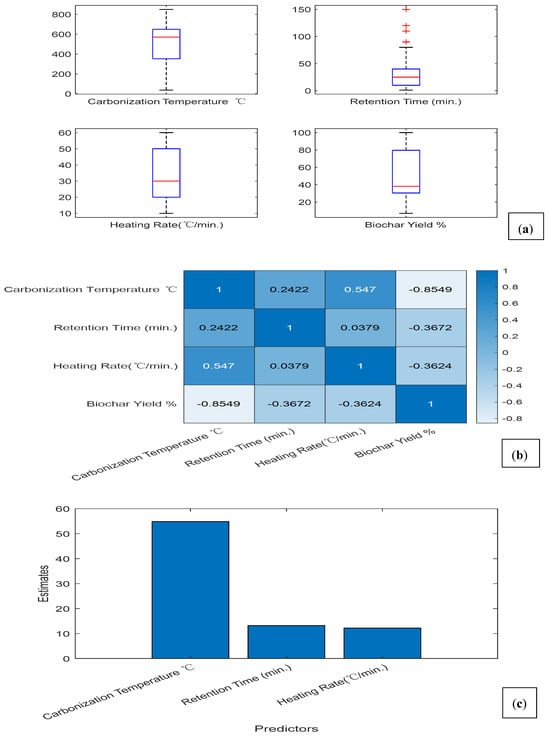
The correlation matrix in Figure 1a quantitatively presents the relationships between the independent variables used in the modeling process and the target variable, biochar yield. The most prominent finding was a strong negative correlation between carbonization temperature and biochar yield (r ≈ −0.8549), indicating that higher temperatures decrease yield by promoting the conversion of solid biomass into liquid and gaseous products. Residence time also exhibited a significant negative correlation (r ≈ −0.3672), suggesting that prolonged exposure accelerates decomposition and further reduces the amount of solid product. Heating rate showed a moderate negative correlation (r ≈ −0.3624), implying that lower heating rates are generally favorable for maintaining higher yields. The presence of moderate correlations among process parameters highlights the potential for interdependency, which supports the use of regularization-based models such as Lasso and ElasticNet for reliable prediction.

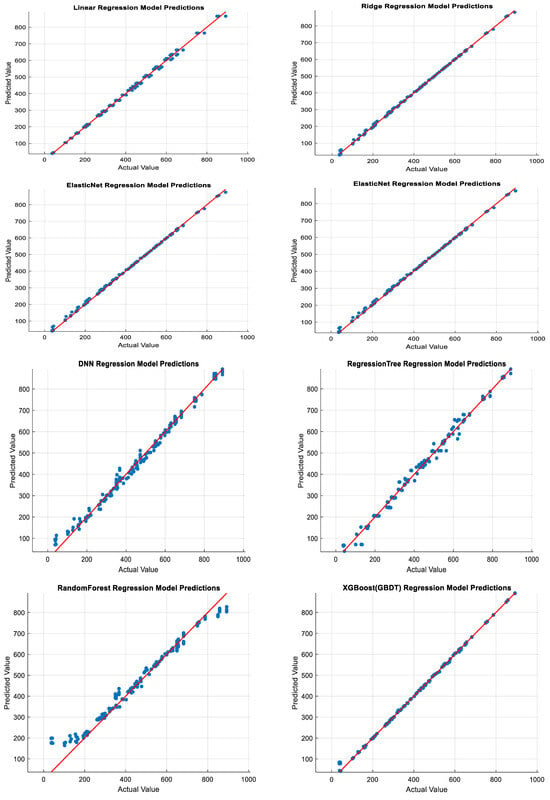
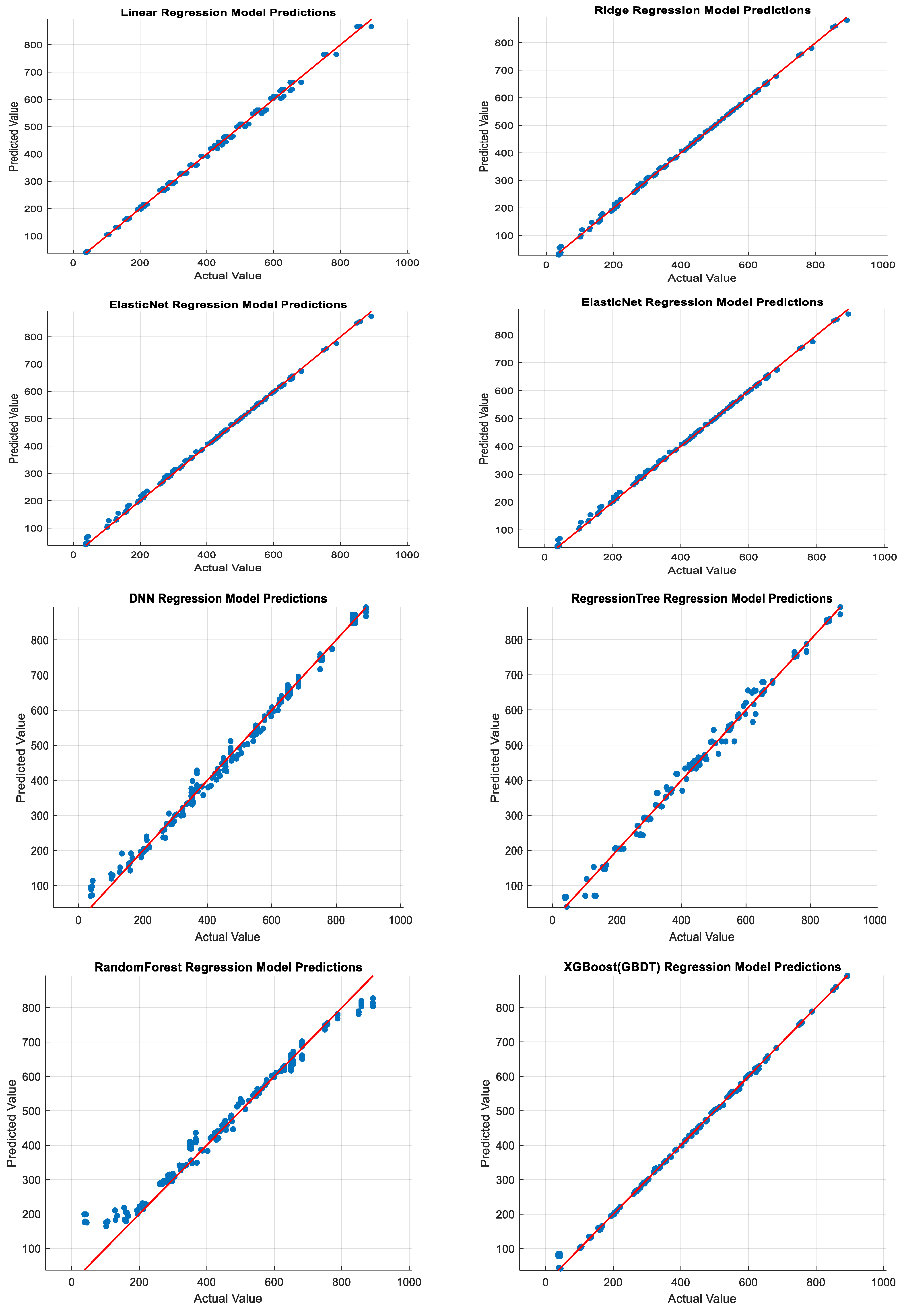
Figure 1b illustrates the predictive performance of the five regression models on the test dataset compared to the actual observed values. The linear regression model captured the general trend but exhibited noticeable deviations in extreme yield cases. Ridge regression provided slightly more stability but retained errors at the distribution tails. Lasso Regression generated closer alignment with the observed data by reducing less influential variables, while ElasticNet produced balanced predictions close to the 1:1 line through the combination of L1 and L2 regularization. The Deep Neural Network (DNN) achieved the highest accuracy on the test dataset, with predicted values closely matching the observed data, demonstrating its ability to capture complex, nonlinear interactions among process parameters.

Figure 1c shows the variable importance scores from the most accurate model, indicating that carbonization temperature was the most influential factor, followed by residence time and heating rate. These three parameters collectively govern the thermal decomposition pathway and the resulting solid product yield. The feature importance analysis derived from the machine learning models revealed that carbonization temperature was the most influential variable, followed by retention time and heating rate. This dominance of temperature is primarily due to its strong physical control over devolatilization, carbonization kinetics, and fixed carbon formation during pyrolysis.

At elevated temperatures (>600 °C), intensified deoxygenation and dehydrogenation reactions lead to the release of oxygen- and hydrogen-rich volatile compounds (e.g., CO, CO₂, H₂O, and light hydrocarbons), resulting in significant mass loss and a reduction in solid biochar yield. Higher temperatures accelerate the release of volatile compounds and promote secondary reactions, which substantially reduce the solid yield, as also indicated by the strong negative correlation (r = −0.85) between temperature and biochar yield. Retention time ranked as the second most influential parameter. A moderate residence period (10–15 min) ensures sufficient carbonization while preventing over-decomposition. However, excessively long retention times at high temperatures can intensify secondary cracking reactions, leading to carbon loss and decreased yield. Compared to conventional slow pyrolysis processes, where residence times are typically on the order of hours, the relatively short residence times employed in this study highlight a more time-efficient conversion process while still achieving comparable biochar yields. Heating rate showed the third-highest contribution. Lower heating rates favor gradual thermal decomposition, allowing more controlled carbonization and thus higher solid yields, whereas rapid heating limits the time for solid formation and enhances volatile release.

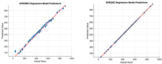
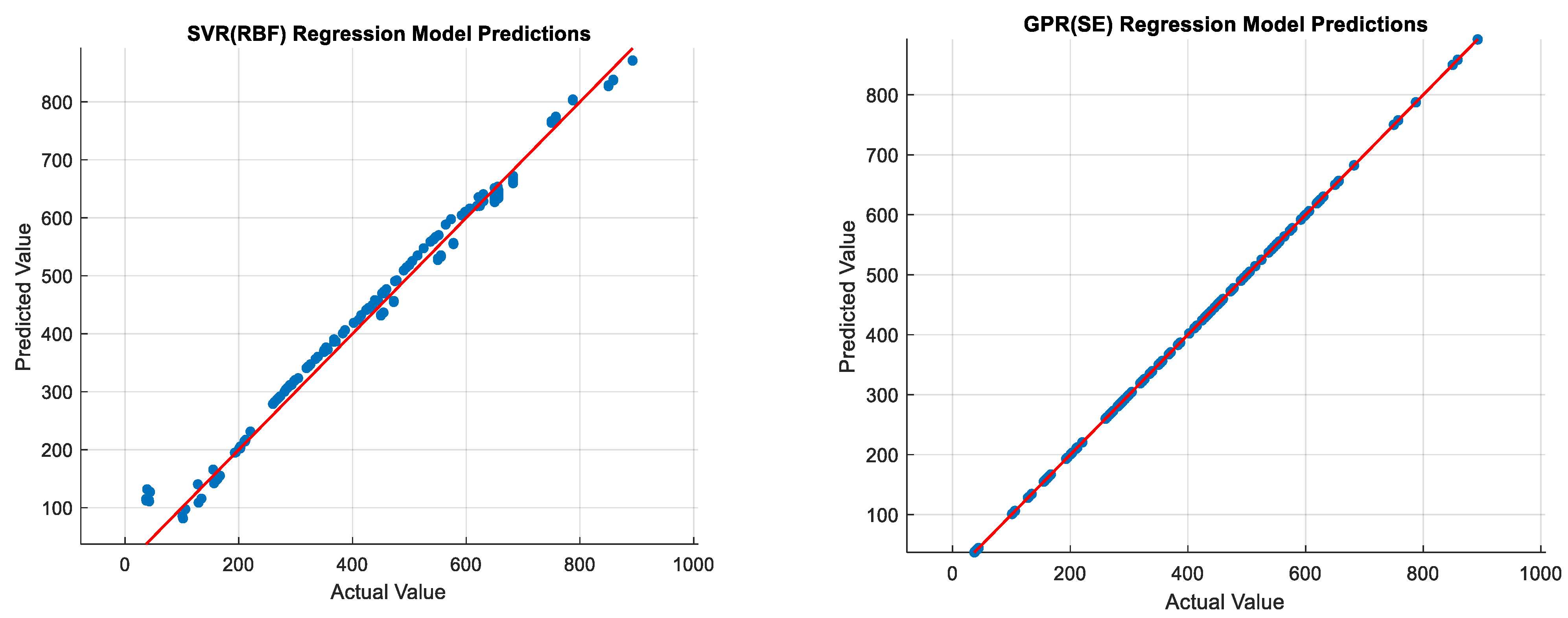
Following the data preprocessing stage, the regression models described in the Methodology Section were applied to predict biochar yield. Their predictive performances were evaluated on the test dataset and compared based on standard regression metrics. The comparative results are presented graphically in Figure 2 and summarized in

Table 2. Ten-fold cross-validation results (mean ± standard deviation) for all regression models for biochar yield prediction.

Model	R2	MAE	MSE	RMSE	MAPE (%)	Adj R2	MFE
Linear	0.9960 ± 0.0012	10.6235 ± 1.0032	148.6751 ± 29.1663	12.1365 ± 1.2384	2.0545 ± 0.1989	0.9953 ± 0.0014	−0.2291 ± 1.9274
Lasso	0.9988 ± 0.0004	4.9019 ± 1.1315	43.8748 ± 17.2635	6.4930 ± 1.3807	1.3009 ± 0.5807	0.9986 ± 0.0005	0.0415 ± 0.9347
Ridge	0.9995 ± 0.0001	3.3649 ± 0.5723	18.9688 ± 6.0470	4.2910 ± 0.7863	1.4248 ± 0.8119	0.9994 ± 0.0001	0.0035 ± 0.6050
ElasticNet	0.9989 ± 0.0004	4.4842 ± 0.7513	43.0428 ± 14.9347	6.4637 ± 1.1848	1.6574 ± 0.8512	0.9987 ± 0.0005	0.0363 ± 0.8437
DNN	0.9920 ± 0.0062	12.4224 ± 4.1834	324.1335 ± 317.5981	16.7537 ± 6.9479	6.0367 ± 5.4990	0.9906 ± 0.0073	−0.8028 ± 5.8727
Regression Tree	0.9848 ± 0.0134	14.2401 ± 5.6105	539.2073 ± 341.0615	22.0977 ± 7.5203	4.8037 ± 2.1056	0.9821 ± 0.0158	−2.9732 ± 5.6975
Random Forest	0.9980 ± 0.0005	5.9284 ± 1.2414	80.9442 ± 35.5867	8.8094 ± 1.9261	2.9050 ± 2.3966	0.9976 ± 0.0006	−0.1292 ± 1.5731
XGBoost (GBDT)	0.9994 ± 0.0010	1.7224 ± 1.4514	30.3119 ± 55.8559	3.8301 ± 4.1690	1.9311 ± 3.3637	0.9993 ± 0.0012	−0.4126 ± 1.4404
SVR (RBF)	0.9882 ± 0.0044	18.6295 ± 2.9955	455.2989 ± 161.0172	21.0073 ± 3.9428	7.7334 ± 5.5752	0.9861 ± 0.0052	3.5003 ± 6.2605
GPR (SE)	0.9999 ± 0.0000	0.0468 ± 0.0075	0.0043 ± 0.0016	0.0642 ± 0.0125	0.0214 ± 0.0155	1.0000 ± 0.0000	−0.0007 ± 0.0157

. Although RMSE provides an error metric in the original unit, MSE is included to emphasize the penalization of larger prediction errors and to provide complementary insight into model performance.

According to the 10-fold cross-validation results in Table 2, the linear regression model showed limited capability in capturing the nonlinear characteristics of the dataset, yielding moderate deviations at extreme biochar yield values (R² = 0.9960 ± 0.0012, RMSE = 12.14 ± 1.24). The Lasso Regression and ElasticNet Regression models improved prediction stability and accuracy through L1 and combined L1–L2 regularization, respectively, achieving R² = 0.9988 ± 0.0004 and 0.9989 ± 0.0004 with correspondingly low RMSE values (6.49 ± 1.38 and 6.46 ± 1.18). The ridge regression model further stabilized the coefficients and provided the lowest bias among the linear approaches (R² = 0.9995 ± 0.0001, RMSE = 4.29 ± 0.79).

Among the nonlinear methods, the Deep Neural Network (DNN) demonstrated strong predictive capability, effectively learning complex parameter interactions (R² = 0.9920 ± 0.0062, MAE = 12.42 ± 4.18, RMSE = 16.75 ± 6.95). However, the best overall predictive performance was obtained with the Gaussian Process Regression (GPR, SE kernel), which achieved near-perfect predictive accuracy within the studied dataset (R² = 0.9999 ± 0.0000, MAE = 0.0468 ± 0.0075, RMSE = 0.0642 ± 0.0125).

Tree-based ensemble methods, including Random Forest (R² = 0.9980 ± 0.0005) and XGBoost (GBDT) (R² = 0.9994 ± 0.0010), also provided highly accurate predictions, confirming their robustness for tabular, nonlinear datasets. The Regression Tree alone exhibited greater variability across folds (R² = 0.9848 ± 0.0134), while the SVR (RBF) model yielded comparatively lower accuracy (R² = 0.9882 ± 0.0044). Overall, the nonlinear and ensemble-based algorithms—particularly GPR and XGBoost—outperformed the linear counterparts, indicating that biochar yield is governed by complex, nonlinear relationships among process parameters.

For GPR models, z-score standardization improved model stability and convergence by ensuring that input variables were on a comparable scale, while also preventing data leakage by computing normalization parameters exclusively from the training data. In contrast, tree-based and linear models (e.g., Random Forest and Regression Tree) demonstrated stable performance without normalization, consistent with their scale-invariant nature. These findings confirm that model-specific preprocessing plays a critical role in achieving reliable predictions within the studied experimental domain, although further validation is required to assess broader generalizability.

As summarized in

Table 3. Summary of recent machine learning-based biochar modeling studies.

Author (Year)	Objective	Data Type/Input Parameters	Applied ML Models	Best Model/Performance
Li et al. (2021) [40]	To predict char yield from lignocellulosic biomass via slow pyrolysis	393–422 literature data: temperature, residence time, particle size, fixed carbon, ash, etc.	Multiple nonlinear regression (MnLR), ANN	ANN: R2 = 0.951 (ash), >0.75 for all outputs
Khan et al. (2022) [41]	To predict biochar yield using ANN with metaheuristic optimization	Biomass properties and pyrolysis parameters	ANN with Rao-2, GA, PSO optimization	ANN–Rao-2: R2 ≈ 0.93, RMSE ≈ 1.74%
Kanthasamy et al. (2023) [42]	To model biochar production from agricultural wastes using data-driven methods	Temperature, heating rate, residence time, N2 flow rate	SVM, GPR, ANN	ANN: R2 > 0.9
Hai et al. (2023) [24]	To predict biochar yield and SSA for 46 biomass types using ML	14 inputs: temperature, ash, fixed carbon, volatile matter, etc.	RF, SVR, ANN, LR, kNN	RF: R2 = 0.85, lowest RMSE
Wang et al. (2024) [43]	To determine the effects of pyrolysis parameters on biochar yield via multi-output ANN	Large dataset: temperature, time, N content, fixed carbon	ANN, RF	ANN: R2 = 0.95, RMSE = 3.6
Ma et al. (2023) [22]	To analyze 13 variables in slow pyrolysis using ML models	Pearson-selected 13 features (biomass + pyrolysis)	GBDT, LM-BP NN, RF, SVR	GBDT and LM-BP NN: R2 > 0.9 (train), >0.8 (test)
Zhao et al. (2025) [44]	To predict biochar yield using classified biomass data	Three classification types (structure, plant, volatile/fixed ratio)	RF, XGBoost, DNN	XGBoost: Avg R2 = 0.883, reduced MAE and RMSE
Bachurin et al. (2025) [45]	To predict product yield ratios from full-scale pyrolysis experiments	750 experimental data: temperature, composition, physical properties	ANN, other NN models	NN: R2 = 0.74, RMSE = 4.58
Bhushan et al. (2025) [46]	To optimize walnut shell pyrolysis parameters for bio-oil and biochar	Temperature, heating rate, inert gas flow rate	RSM + ML (decision tree)	RSM: R2 = 0.92, DT: R2 = 0.74
In this study	To model experimentally obtained biochar yield from tea-brewing waste and almond husk under various pyrolysis conditions using ML	Experimental data: temperature (37–850 °C), residence time (1–150 min), heating rate (10–60 °C/min)	Linear, Ridge, Lasso, ElasticNet, Regression Tree, RF, XGBoost, SVR, GPR, DNN	GPR: R2 = 0.9999, RMSE = 0.064; DNN: R2 = 0.99997, RMSE = 2.54

, most recent studies have explored the application of machine learning to predict biochar yield or kinetic behavior under varying pyrolysis conditions [22,24,40,41,42,43,44,45,46]. Among these, models such as ANN, Random Forest, and XGBoost consistently achieved higher predictive accuracy (R² > 0.85), indicating their robustness in capturing nonlinear dependencies between process parameters and yield. The higher predictive performance observed in this study can be attributed to three main factors. First, the models were trained on a controlled and consistent experimental dataset generated under well-defined conditions, reducing noise and variability compared to heterogeneous literature-based datasets. Second, Gaussian Process Regression (GPR), due to its probabilistic nature and flexibility, is particularly well-suited for small and well-structured datasets, enabling highly accurate modeling of complex nonlinear relationships. Third, the use of 10-fold cross-validation with unseen test data in each iteration ensured that the reported results reflect strong generalization capability rather than overfitting. While studies such as those performed by Li et al. (2021) [40] and Khan et al. (2022) [41] demonstrated the potential of ANN-based hybrid or optimized frameworks, others like those conducted by Hai et al. (2023) [24] and Zhao et al. (2025) [44] emphasized the importance of data preprocessing, feature selection, and biomass classification in improving model performance. In contrast to most of these works, which rely on literature-based or compiled datasets, the present study integrates experimentally generated biochar data with ten distinct ML regression models, providing a hybrid experimental–computational framework. This integration enhances model interpretability and generalization while establishing a methodological bridge between physical experiments and predictive data-driven modeling. Notably, the Gaussian Process Regression (GPR) and Deep Neural Network (DNN) models achieved exceptional accuracy (R² ≈ 0.9999), establishing a robust and generalizable prediction approach for optimizing biochar production under varying pyrolysis conditions.

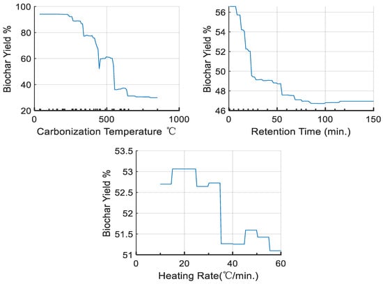
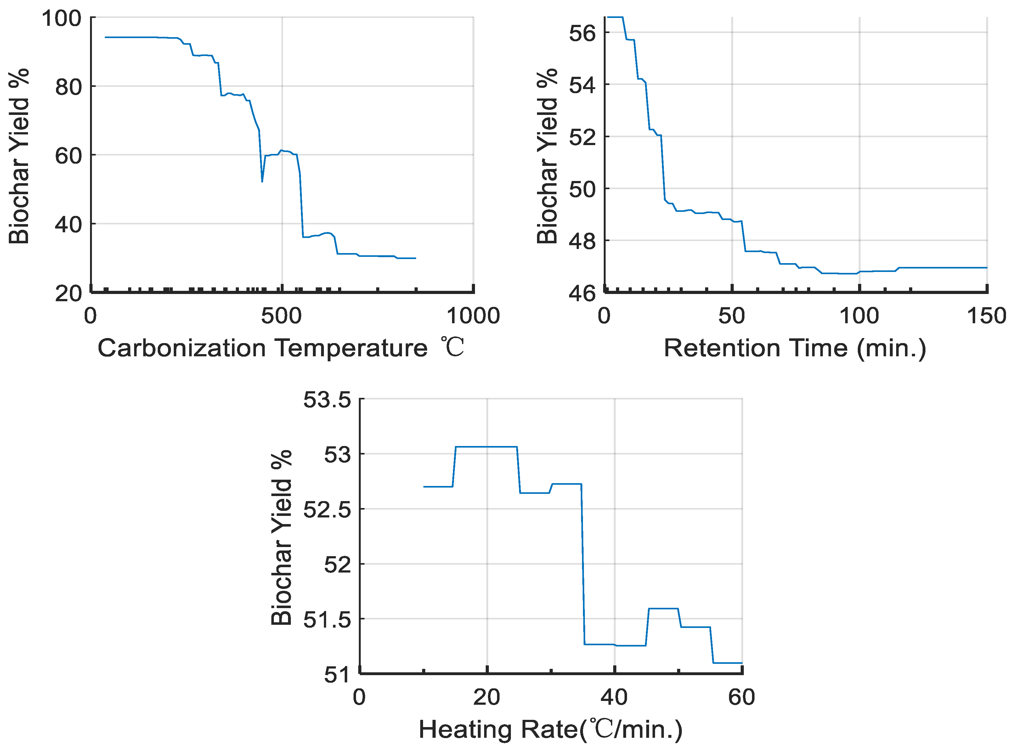
In Figure 3, the effect of each independent variable on biochar yield is presented using a partial dependence plot based on the relationships learned by the machine learning model. This analysis shows what kind of change the model predicts in biochar yield output when the value of a single variable is changed while all other variables remain constant.

Carbonization Temperature (°C)–Biochar Yield Relationship: According to the relationship learned by the model, as temperature increases, biochar yield decreases sharply, especially in the 300–600 °C range, where yield decreases from 60 to 40. This indicates that as carbonization temperature increases, the amount of solid product decreases due to the conversion of organic components into volatile compounds. This behavior is mainly attributed to the thermal decomposition of hemicellulose and cellulose, which predominantly occurs within this temperature range. Beyond 600 °C, yield tends to stabilize, suggesting that the majority of easily decomposable components have already been volatilized. However, lignin—a more thermally resistant component—continues to degrade over a broader temperature range, extending up to approximately 800–900 °C. This gradual degradation of lignin contributes to further structural rearrangement, aromatization, and carbon enrichment of the solid phase, rather than a significant additional loss in mass.

Pyrolysis temperature affects not only the yield but also the physicochemical properties of biochar, including elemental composition, surface area, pore structure, and functional groups [47,48]. Similar to the results obtained in this study, many studies have reported that pyrolysis temperature is inversely proportional to biochar yield and directly related to bio-oil production. For instance, increasing the temperature from 400 °C to 700 °C has been shown to reduce biochar yield by approximately 10–30% [49]. In the present study, a more pronounced decrease was observed, with biochar yield dropping from approximately 60% to 40% within the 300–600 °C range, corresponding to a reduction of about 20 percentage points.

Heating Rate (°C/min)–Biochar Yield Relationship: Heating rate is an important parameter affecting the pyrolysis products and their composition. The model revealed a moderate but distinct influence of heating rate on biochar yield.

At lower heating rates, particularly in the range of 10–20 °C/min, the highest yields (≈52–55%) were achieved, especially when combined with optimal carbonization temperature (400–500 °C) and residence time (10–15 min). This range allows for gradual devolatilization and improved retention of solid carbon in the biochar. As the heating rate increases above 40 °C/min, yield begins to decline steadily, with losses of up to 10–15 percentage points compared to the optimal range. At the maximum tested rate of 60 °C/min, the rapid temperature rise accelerates volatile release and limits the time for solid-phase reactions, resulting in the lowest observed yields in the dataset. Under such conditions, limited heat transfer within the particle and increased thermal gradients promote thermal fragmentation, favoring the formation of condensable vapors (bio-oil) rather than solid biochar.

These results indicate that controlling heating rate within a moderate range is a key operational strategy for maximizing biochar production efficiency. Higher heating rates promote decomposition pathways that increase liquid and gas yields, whereas lower heating rates favor secondary char-forming reactions and enhance biochar production [50]. Similar to our findings, it has been reported that increasing the heating rate to 30–50 °C/min and operating at 400–500 °C leads to a decrease in biochar yield [51].

Retention Time (min)–Biochar Yield Relationship: Retention time is an important factor for the distribution and composition of pyrolysis products. Short residence times favor liquid and gaseous products, while longer residence times increase biochar yield by providing greater repolymerization possibilities [52]. While an increase in retention time initially keeps the biochar yield relatively constant, a significant decrease in biochar yield is observed after 15 min. For example, while the yield remains around 50% between 0 and 10 min, it drops below 40% after 30 min. This indicates that prolongation of the carbonization time leads to increased fragmentation and transition to the gas phase. Similar results have been reported in the literature, supporting our findings [53,54], demonstrating that residence time and biochar yield are inversely related.

These evaluations have revealed that the most critical factor affecting biochar yield is carbonization temperature, followed by residence time and heating rate. Optimizing these process parameters plays a significant role in enhancing the efficiency of biochar production.

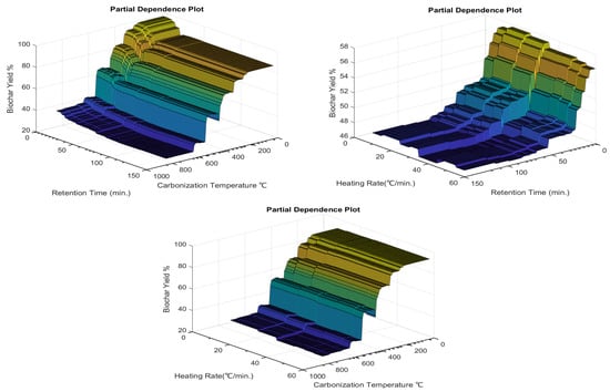
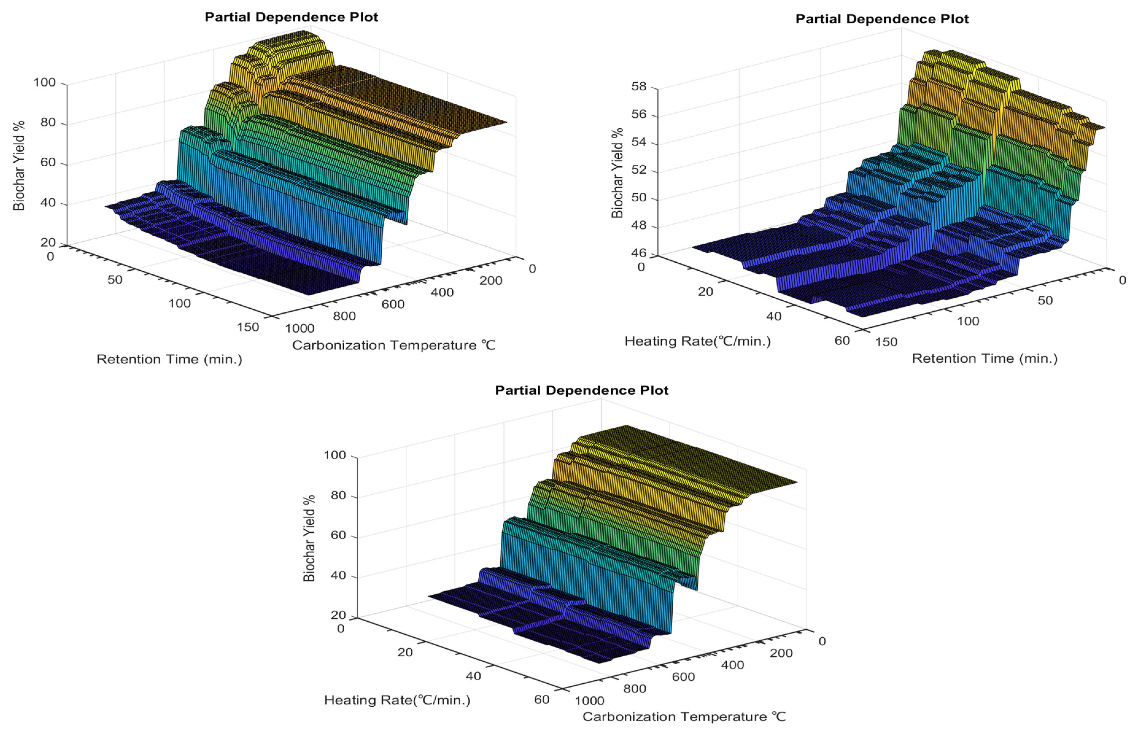
Machine learning models can learn not only the effects of individual variables on the target variable but also the complex interactions between pairs of variables. The two-variable partial dependence analyses (2D partial dependence plots) in Figure 4 illustrate how biochar yield changes when two independent variables vary simultaneously while all others are held constant. These plots are essential for visualizing nonlinear relationships and identifying synergistic or antagonistic effects among process parameters.

Carbonization Temperature and Residence Time: Pyrolysis parameters exhibit synergistic effects. The model shows a pronounced decline in yield when both temperature and residence time are high. Specifically, yields drop below 40% at temperatures above 550 °C combined with residence times longer than 25 min. This region represents severe pyrolysis conditions, where prolonged heating accelerates thermal decomposition and shifts product distribution toward gases and liquids. Conversely, the range of 350–450 °C and 10–15 min residence time are identified as optimal conditions, producing yields of approximately 52–55%.

Although some studies have reported that higher temperatures combined with longer residence times may increase biochar yield [55], this behavior is strongly dependent on biomass type and process conditions. In the present study, the combined effect of high temperature and extended residence time led to enhanced devolatilization, secondary cracking, and carbon loss, resulting in reduced biochar yield. This trend is consistent with findings indicating that prolonged residence time at elevated temperatures promotes further degradation of solid carbon into gaseous and liquid products [56]. Therefore, the apparent discrepancy can be attributed to differences in feedstock composition and operating conditions, highlighting the importance of process-specific optimization.

Carbonization Temperature and Heating Rate: A clear interaction is observed between these parameters. At moderate temperatures (400–500 °C), low heating rates (10–20 °C/min) produce the highest yields (≈54–55%). However, at higher temperatures (>600 °C), increasing the heating rate above 30 °C/min accelerates volatile release and significantly reduces yield to below 40%. This suggests that low heating rates help preserve solid carbon content by allowing more gradual devolatilization, particularly in the optimal temperature range.

Heating Rate and Residence Time: Heating rate alone generally has little effect on pyrolysis products. Therefore, it has been stated in the literature that its evaluation should be considered as a function of retention time and temperature [57]. The interaction between heating rate and residence time shows that the best yields are achieved at low heating rates (10–20 °C/min) combined with moderate residence times (10–15 min), resulting in yields around 53–54%. When both heating rate exceeds 40 °C/min and residence time exceeds 25 min, yield declines sharply to below 35%, indicating that prolonged exposure at rapid heating accelerates carbon loss. In contrast, shorter residence times (<10 min) can partially mitigate the negative impact of higher heating rates, but only when combined with moderate temperatures.

Accordingly, pyrolysis conditions influence the distribution of products among solid, liquid, and gaseous phases, as reported in the literature [57]. However, in the present study, the machine learning models were developed specifically to predict biochar yield. Therefore, the discussion is primarily focused on the solid product, while observations regarding liquid and gaseous products are provided only as general background information. From this perspective, the decrease in biochar yield at higher temperatures and heating rates can be attributed to the enhanced formation of volatile products, which reduces the amount of solid residue.

Overall, the 2D interaction analyses confirm that carbonization temperature is the dominant factor, but its effect is strongly modulated by heating rate and residence time. Extreme values of any two parameters simultaneously tend to suppress yield, while balanced, moderate settings across all three lead to optimal biochar production. These findings underscore the importance of multi-parameter optimization and demonstrate that the best-performing model, GPR, effectively captured and generalized the complex multidimensional interactions governing biochar yield in the pyrolysis system.

4. Conclusions

This study demonstrated that biochar yield from tea-brewing residues and almond husks is governed by strong nonlinear interactions among carbonization temperature, residence time, and heating rate. Comparative modeling results confirmed that conventional linear regressors were limited in capturing these complex dependencies, whereas regularized and ensemble-based machine learning models significantly improved predictive accuracy and robustness. Among the evaluated approaches, Gaussian Process Regression (GPR) achieved the highest predictive performance within the studied dataset (R² = 0.9999, RMSE = 0.064), followed by Deep Neural Networks (DNNs) and Extreme Gradient Boosting (XGBoost), highlighting the effectiveness of advanced nonlinear and probabilistic models for biochar yield prediction.

Sensitivity and interaction analyses identified carbonization temperature as the dominant controlling parameter, with pronounced yield reductions observed above 600 °C. Optimal biochar yields of approximately 52–55% were consistently obtained at moderate temperatures (400–500 °C) and short residence times (10–15 min), while lower heating rates contributed to improved yield stability.

From a practical perspective, the selection of an appropriate machine learning model should be guided by dataset size and complexity. For relatively small experimental datasets, probabilistic models such as GPR can provide high predictive accuracy and stable performance. For medium-sized datasets, ensemble methods such as Random Forest and XGBoost offer a balance between accuracy and computational efficiency. In contrast, for large-scale datasets, deep learning approaches such as DNN are more suitable due to their ability to capture highly complex nonlinear relationships.

Overall, the findings demonstrate that data-driven modeling frameworks, particularly GPR- and DNN-based approaches, provide reliable and interpretable tools for optimizing pyrolysis conditions within the studied experimental domain. This integrated experimental–computational strategy contributes to the valorization of lignocellulosic waste; however, further validation using diverse biomass types and comprehensive sustainability assessments (e.g., LCA or TEA) are required to support broader applicability.

References

- McKendry, P. Energy production from biomass (part 1): Overview of biomass. Bioresour. Technol. 2002, 83, 37–46. [Google Scholar] [CrossRef] [Scilit]
- McKendry, P. Energy production from biomass (part 2): Conversion technologies. Bioresour. Technol. 2002, 83, 47–54. [Google Scholar] [CrossRef] [Scilit]
- Taşar, Ş. Developing a new model equation between proximate compositions of biomass resources and upper heat values and investigation of the model equation’s success. Artvin Çoruh Univ. J. For. Fac. 2021, 22, 42–51. [Google Scholar]
- Li, W.; Xu, Y.; Wang, G.; Xu, T.; Wang, K.; Zhai, S.; Si, C. Sustainable carbon-based catalyst materials derived from lignocellulosic biomass for energy storage and conversion: Atomic modulation and properties improvement. Carbon Energy 2025, 7, e708. [Google Scholar] [CrossRef] [Scilit]
- Ungureanu, N.; Vlăduț, N.V.; Biriș, S.Ș.; Gheorghiță, N.E.; Ionescu, M. Biomass pyrolysis pathways for renewable energy and sustainable resource recovery: A critical review of processes, parameters, and product valorization. Sustainability 2025, 17, 7806. [Google Scholar] [CrossRef] [Scilit]
- González, J.F.; González-Garcı́a, C.M.; Ramiro, A.; González, J.; Sabio, E.; Gañán, J.; Rodrı́guez, M.A. Combustion optimisation of biomass residue pellets for domestic heating with a mural boiler. Biomass Bioenergy 2004, 27, 145–154. [Google Scholar] [CrossRef] [Scilit]
- Kumari, R.; Dwivedi, N.; Meehnian, H. Industrial Framework for Net Zero Emission Transition in Emerging Economies. In Sustainable Biotechnological Remedial Frameworks for the Rejuvenation of Heavily Polluted Environments; CRC Press: Boca Raton, FL, USA, 2025; pp. 387–412. [Google Scholar]
- BEPA-T. C. Ministry of Energy and Natural Resources General Directorate of Energy Affairs, Biomass Energy Potential Atlas. 2025. Available online: https://bepa.enerji.gov.tr/ (accessed on 20 December 2025).
- Tan, M.; Li, H.; Huang, Z.; Wang, Z.; Xiong, R.; Jiang, S.; Zhang, J.; Wu, Z.; Li, C.; Luo, L. Comparison of atmospheric and gas-pressurized oxidative torrefaction of heavy-metal-polluted rice straw. J. Clean. Prod. 2021, 283, 124636. [Google Scholar] [CrossRef] [Scilit]
- Ministry of Agriculture and Forestry. Tea Market Report (July 2025); General Directorate of Agricultural Research and Policies (TEPGE): Ankara, Turkey, 2025. [Google Scholar]
- Turkish Statistical Institute (TURKSTAT). Crop Production Statistics; Turkish Statistical Institute (TURKSTAT): Ankara, Turkey, 2025. [Google Scholar]
- Al-Widyan, M.I.; Tashtoush, G.; Hamasha, A.M. Combustion and emissions of pulverized olive cake in tube furnace. Energy Convers. Manag. 2006, 47, 1588–1596. [Google Scholar] [CrossRef] [Scilit]
- Yaman, S. Pyrolysis of biomass to produce fuels and chemical feedstocks. Energy Convers. Manag. 2004, 45, 651–671. [Google Scholar] [CrossRef] [Scilit]
- Li, J.; Chen, Y.; Yang, H.; Zhu, D.; Chen, X.; Wang, X.; Chen, H. Correlation of feedstock and bio-oil compound distribution. Energy Fuels 2017, 31, 7093–7100. [Google Scholar] [CrossRef] [Scilit]
- Oasmaa, A.; Solantausta, Y.; Arpiainen, V.; Kuoppala, E.; Sipila, K. Fast pyrolysis bio-oils from wood and agricultural residues. Energy Fuels 2010, 24, 1380–1388. [Google Scholar]
- Cao, H.; Xin, Y.; Yuan, Q. Prediction of biochar yield from cattle manure pyrolysis via least squares support vector machine intelligent approach. Bioresour. Technol. 2016, 202, 158–164. [Google Scholar] [CrossRef] [Scilit]
- Sun, Y.; Liu, L.; Wang, Q.; Yang, X.; Tu, X. Pyrolysis products from industrial waste biomass based on a neural network model. J. Anal. Appl. Pyrolysis 2016, 120, 94–102. [Google Scholar] [CrossRef] [Scilit]
- Naqvi, S.R.; Hameed, Z.; Tariq, R.; Taqvi, S.A.; Ali, I.; Niazi, M.B.K.; Noor, T.; Hussain, A.; Iqbal, N.; Shahbaz, M. Synergistic effect on co-pyrolysis of rice husk and sewage sludge by thermal behavior, kinetics, thermodynamic parameters and artificial neural network. Waste Manag. 2019, 85, 131–140. [Google Scholar] [CrossRef] [Scilit]
- Xing, J.; Luo, K.; Wang, H.; Gao, Z.; Fan, J. A comprehensive study on estimating higher heating value of biomass from proximate and ultimate analysis with machine learning approaches. Energy 2019, 188, 116077. [Google Scholar] [CrossRef] [Scilit]
- Tang, Q.; Chen, Y.; Yang, H.; Liu, M.; Xiao, H.; Wu, Z.; Chen, H.; Naqvi, S.R. Prediction of bio-oil yield and hydrogen contents based on machine learning method: Effect of biomass compositions and pyrolysis conditions. Energy Fuels 2020, 34, 11050–11060. [Google Scholar] [CrossRef] [Scilit]
- Panicker, T.F.; Sarkar, D.; Krishna, R.; Mishra, R.K.; Manjeshwar, S.K.; Sharma, A. A machine learning-assisted prediction of potential biochar yield subjected to the physicochemical properties of biomass. Fuel 2026, 409, 137836. [Google Scholar] [CrossRef] [Scilit]
- Ma, J.; Zhang, S.; Liu, X.; Wang, J. Machine learning prediction of biochar yield based on biomass characteristics. Bioresour. Technol. 2023, 389, 129820. [Google Scholar] [CrossRef] [Scilit]
- Li, Y.; Gupta, R.; You, S. Machine learning assisted prediction of biochar yield and composition via pyrolysis of biomass. Bioresour. Technol. 2022, 359, 127511. [Google Scholar] [CrossRef] [Scilit]
- Hai, A.; Bharath, G.; Patah, M.F.A.; Daud, W.M.A.W.; Show, P.; Banat, F. Machine learning models for the prediction of total yield and specific surface area of biochar derived from agricultural biomass by pyrolysis. Environ. Technol. Innov. 2023, 30, 103071. [Google Scholar] [CrossRef] [Scilit]
- ASTM E872–82; Standard Test Method for Volatile Matter in the Analysis of Particulate Wood Fuels. American Society for Testing and Materials: Philadelphia, PA, USA, 1982.
- ASTM E1755–95; Standard Test Method for Ash in Biomass. American Society for Testing and Materials: Philadelphia, PA, USA, 1995.
- ASTM D3176; Standard Practice for Ultimate Analysis of Coal and Coke (ASTM D3176-15). ASTM International, American Society for Testing and Materials: Philadelphia, PA, USA, 2009.
- ASTM E870–82; Standard Test Methods for Analysis of Wood Fuels. American Society for Testing and Materials: Philadelphia, PA, USA, 2006.
- Jiang, H.; Zheng, Y.; Dong, Z.; Ming, H.; Guo, X.; Cheng, L.; Zhang, L. TG-FTIR Analysis of Co-Pyrolysis Behavior Between Petroleum Coke and Model Lignocellulosic Biomass. J. Energy Inst. 2025, 122, 102223. [Google Scholar] [CrossRef] [Scilit]
- Brebu, M.; Butnaru, E.; Stoleru, E.; Sim, S.F. Source discrimination by classical characterization methods, FTIR and statistical analysis–a prerequisite for thermochemical conversion of agriculture biomass residues by torrefaction and pyrolysis. Energy 2025, 334, 137637. [Google Scholar] [CrossRef] [Scilit]
- Tiwari, M.; Dirbeba, M.J.; Lehmusto, J.; Yrjas, P.; Vinu, R. Analytical and applied pyrolysis of challenging biomass feedstocks: Effect of pyrolysis conditions on product yield and composition. J. Anal. Appl. Pyrolysis 2024, 177, 106355. [Google Scholar] [CrossRef] [Scilit]
- Taşar, Ş. Estimation of pyrolysis liquid product yield and its hydrogen content for biomass resources by combined evaluation of pyrolysis conditions with proximate–ultimate analysis data: A machine learning application. J. Anal. Appl. Pyrolysis 2022, 165, 105546. [Google Scholar] [CrossRef] [Scilit]
- Tang, Q.; Chen, Y.; Yang, H.; Liu, M.; Xiao, H.; Wang, S.; Chen, H.; Naqvi, S.R. Machine learning prediction of pyrolytic gas yield and compositions with feature reduction methods: Effects of pyrolysis conditions and biomass characteristics. Bioresour. Technol. 2021, 339, 125581. [Google Scholar] [CrossRef] [Scilit]
- Pahnila, M.; Koskela, A.; Sulasalmi, P.; Fabritius, T. A review of pyrolysis technologies and the effect of process parameters on biocarbon properties. Energies 2023, 16, 6936. [Google Scholar] [CrossRef] [Scilit]
- Tumuluru, J.S.; Ghiasi, B.; Soelberg, N.R.; Sokhansanj, S. Biomass torrefaction process, product properties, reactor types, and moving bed reactor design concepts. Front. Energy Res. 2021, 9, 728140. [Google Scholar] [CrossRef] [Scilit]
- Taşar, Ş. Thermal conversion behavior of cellulose and hemicellulose fractions isolated from tea leaf brewing waste: Kinetic and thermodynamic evaluation. Biomass Convers. Biorefinery 2022, 12, 2935–2947. [Google Scholar] [CrossRef] [Scilit]
- Taşar, Ş.; Özer, A. A comparative study of hemicellulose isolation with hot water, alkaline, and delignification methods from tea leaf brewing waste. Biomass Convers. Biorefinery 2022, 12, 2501–2514. [Google Scholar] [CrossRef] [Scilit]
- Alhaji Mohammed, M.; Basirun, W.J.; Abd Rahman, N.M.M.; Salleh, N. The effect of particle size of almond shell powders, temperature and time on the extraction of cellulose. J. Nat. Fibers 2022, 19, 5577–5587. [Google Scholar] [CrossRef] [Scilit]
- Debevc, S.; Weldekidan, H.; Snowdon, M.R.; Vivekanandhan, S.; Wood, D.F.; Misra, M.; Mohanty, A.K. Valorization of almond shell biomass to biocarbon materials: Influence of pyrolysis temperature on their physicochemical properties and electrical conductivity. Carbon Trends 2022, 9, 100214. [Google Scholar] [CrossRef] [Scilit]
- Li, T.Y.; Xiang, H.; Yang, Y.; Wang, J.; Yildiz, G. Prediction of char production from slow pyrolysis of lignocellulosic biomass using multiple nonlinear regression and artificial neural network. J. Anal. Appl. Pyrolysis 2021, 159, 105286. [Google Scholar] [CrossRef] [Scilit]
- Khan, M.; Ullah, Z.; Mašek, O.; Naqvi, S.R.; Khan, M.N.A. Artificial neural networks for the prediction of biochar yield: A comparative study of metaheuristic algorithms. Bioresour. Technol. 2022, 355, 127215. [Google Scholar] [CrossRef] [Scilit]
- Kanthasamy, R.; Almatrafi, E.; Ali, I.; Sait, H.H.; Zwawi, M.; Abnisa, F.; Peng, L.C.; Ayodele, B.V. Biochar production from valorization of agricultural Wastes: Data-Driven modelling using Machine learning algorithms. Fuel 2023, 351, 128948. [Google Scholar] [CrossRef] [Scilit]
- Wang, Y.; Xu, L.; Li, J.; Ren, Z.; Liu, W.; Ai, Y.; Zhou, Y.; Li, Q.; Zhang, B.; Guo, N.; et al. Multi-output neural network model for predicting biochar yield and composition. Sci. Total Environ. 2024, 945, 173942. [Google Scholar]
- Zhao, C.; Yang, H.; Ma, H.; Chen, A.; Liu, X.; Chen, J. Machine learning prediction of biochar yield based on different classification methods. J. Renew. Sustain. Energy 2025, 17, 053103. [Google Scholar] [CrossRef] [Scilit]
- Bachurin, R.M.; Zakharova, I.G. Artificial Intelligence Methods for Predicting Pyrolysis Product Yields of Lignocellulosic Biomass. In 2025 International Russian Automation Conference (RusAutoCon); IEEE: New York, NY, USA, 2025; pp. 556–560. [Google Scholar]
- Bhushan, D.; Tomar, K.; Mondal, P. Multi-parameter optimization and predictive modeling of pyrolysis of walnut shells in fixed bed reactor using response surface methodology and machine learning algorithms. J. Anal. Appl. Pyrolysis 2025, 192, 107242. [Google Scholar] [CrossRef] [Scilit]
- Al-Rumaihi, A.; Shahbaz, M.; Mckay, G.; Mackey, H.; Al-Ansari, T. A review of pyrolysis technologies and feedstock: A blending approach for plastic and biomass towards optimum biochar yield. Renew. Sustain. Energy Rev. 2022, 167, 112715. [Google Scholar] [CrossRef] [Scilit]
- Dhyani, V.; Bhaskar, T. A comprehensive review on the pyrolysis of lignocellulosic biomass. Renew. Energy 2018, 129, 695–716. [Google Scholar] [CrossRef] [Scilit]
- Choi, H.S.; Choi, Y.S.; Park, H.C. Fast pyrolysis characteristics of lignocellulosic biomass with varying reaction conditions. Renew. Energy 2012, 42, 131–135. [Google Scholar] [CrossRef] [Scilit]
- Ahmad, J.; Patuzzi, F.; Rashid, U.; Shahabz, M.; Ngamcharussrivichai, C.; Baratieri, M. Exploring untapped effect of process conditions on biochar characteristics and applications. Environ. Technol. Innov. 2021, 21, 101310. [Google Scholar] [CrossRef] [Scilit]
- Aysu, T.; Durak, H.; Güner, S.; Bengü, A.Ş.; Esim, N. Bio-oil production via catalytic pyrolysis of Anchusa azurea: Effects of operating conditions on product yields and chromatographic characterization. Bioresour. Technol. 2016, 205, 7–14. [Google Scholar] [CrossRef] [Scilit] [PubMed]
- Chen, W.H.; Farooq, W.; Shahbaz, M.; Naqvi, S.R.; Ali, I.; Al-Ansari, T.; Amin, N.A.S. Current status of biohydrogen production from lignocellulosic biomass, technical challenges and commercial potential through pyrolysis process. Energy 2021, 226, 120433. [Google Scholar] [CrossRef] [Scilit]
- Sun, J.; He, F.; Pan, Y.; Zhang, Z. Effects of pyrolysis temperature and residence time on physicochemical properties of different biochar types. Acta Agric. Scand. Sect. B Soil Plant Sci. 2017, 67, 12–22. [Google Scholar] [CrossRef] [Scilit]
- Sharuddin, S.D.A.; Abnisa, F.; Daud, W.M.A.W.; Aroua, M.K. A review on pyrolysis of plastic wastes. Energy Convers. Manag. 2016, 115, 308–326. [Google Scholar] [CrossRef] [Scilit]
- Fassinou, W.F.; Van de Steene, L.; Toure, S.; Volle, G.; Girard, P. Pyrolysis of Pinus pinaster in a two-stage gasifier: Influence of processing parameters and thermal cracking of tar. Fuel Process. Technol. 2009, 90, 75–90. [Google Scholar] [CrossRef] [Scilit]
- Liang, C.; Gascó, G.; Fu, S.; Méndez, A.; Paz-Ferreiro, J. Biochar from pruning residues as a soil amendment: Effects of pyrolysis temperature and particle size. Soil Tillage Res. 2016, 164, 3–10. [Google Scholar]
- Bridgwater, A.V.; Toft, A.J.; Brammer, J.G. A techno-economic comparison of power production by biomass fast pyrolysis with gasification and combustion. Renew. Sustain. Energy Rev. 2002, 6, 181–246. [Google Scholar] [CrossRef] [Scilit]
Disclaimer/Publisher’s Note: The statements, opinions and data contained in all publications are solely those of the individual author(s) and contributor(s) and not of MDPI and/or the editor(s). MDPI and/or the editor(s) disclaim responsibility for any injury to people or property resulting from any ideas, methods, instructions or products referred to in the content. |
© 2026 by the authors. Licensee MDPI, Basel, Switzerland. This article is an open access article distributed under the terms and conditions of the Creative Commons Attribution (CC BY) license.