Speed Limit Strategies for Median Crossover Sections in Freeway Reconstruction and Expansion: A Case Study of a Four-to-Eight-Lane Expansion Project in a Plain Area

Abstract

During freeway reconstruction and expansion, median crossover sections where traffic is maintained during construction are vulnerable to changes in lane configuration, abrupt geometric changes, and construction interference. These factors may lead to safety risks and operational efficiency losses. Existing studies have mainly relied on microscopic traffic simulation to evaluate speed limit schemes, while engineering costs, environmental impacts, driver responses, and policy constraints have rarely been considered in an integrated manner. This study proposes a two-stage evaluation framework that integrates VISSIM microscopic traffic simulation, the Entropy Weight Method–Technique for Order Preference by Similarity to an Ideal Solution (EWM–TOPSIS), and the Fuzzy Analytic Hierarchy Process (FAHP). A four to eight-lane freeway expansion project in a plain area of northern China is used as the case study. Field speed data from a representative median crossover section are used for model calibration and speed-pattern analysis. A total of 27 simulation scenarios is then constructed by combining three bottleneck types, three traffic saturation levels, and three speed limit schemes. The EWM–TOPSIS results show that the 80→70 km/h scheme achieves the highest relative closeness in all scenarios. The FAHP evaluation, based on six criteria and 21 indicators, also ranks this scheme first. Its ranking remains unchanged under ±10% criteria weight perturbations. Field speed comparison indicates that vehicles exhibit a deceleration–recovery pattern when passing through the crossover opening. Overall, the 80→70 km/h gradual speed reduction scheme can be regarded as a candidate scheme for work zones with similar median crossover configurations. Under localized calibration conditions, it can provide decision-making support for reducing operational disturbances, fuel consumption, and external impacts associated with crash risk.

1. Introduction

In China, as society and the economy rapidly develop, freeway construction is shifting from a stage dominated by new construction to a sustainable stage focused on upgrading existing infrastructure [1]. As a result, older freeways are increasingly unable to meet growing traffic demands, requiring reconstruction or expansion to enhance their capacity and service levels. To minimize the impact of construction on surrounding road networks, the “maintaining traffic during construction” model, which ensures uninterrupted traffic during the expansion or reconstruction process, has become the primary approach for freeway projects in China.

During freeway reconstruction and expansion, staged and alternating construction across different carriageways often requires temporary openings in the original central median. These openings allow traffic to shift from one carriageway to the other, thereby forming median crossover sections. Affected by changes in lane configuration, abrupt geometric changes, inadequate speed control, and construction interference, these sections often become bottleneck areas with frequent crashes and reduced operational efficiency during freeway reconstruction and expansion [2,3]. For such complex work zones, optimizing traffic organization through work zone layout, speed limits, and traffic safety facilities has become an important management measure [4,5]. Among these measures, speed limits play a central role in balancing safety and efficiency. Their rational design directly affects vehicle speed coordination, driver adaptability, and the overall effectiveness of traffic organization during construction.

Existing studies on work zone speed limits and speed control have examined safety risk, operational efficiency, dynamic speed limits, and traffic simulation evaluation. These studies provide a foundation for understanding how speed differences, speed dispersion, abrupt geometric changes, and traffic flow disturbances affect operational safety in work zones. However, for median crossover sections in freeway reconstruction and expansion, relying solely on a single safety indicator or a single simulation-based evaluation remains insufficient. Such an approach cannot fully reflect the comprehensive performance of speed limit schemes in terms of engineering implementation, driver behavioral adaptation, environmental impacts, and policy constraints. In complex work zone traffic organization, a scheme with better technical indicators may not necessarily be equally suitable from a comprehensive management perspective. Therefore, the evaluation of speed limit schemes should consider multiple objectives, including safety, efficiency, economic cost, environment, driving behavior, and social policy.

Based on this background, this study focuses on a median crossover section in a four-to-eight-lane freeway expansion project in a plain area of northern China. VISSIM microscopic traffic simulation scenarios are constructed to cover different bottleneck characteristics, traffic saturation levels, and speed limit schemes. A two-stage evaluation framework is then developed by integrating EWM–TOPSIS, which combines the Entropy Weight Method with the Technique for Order Preference by Similarity to an Ideal Solution, and the Fuzzy Analytic Hierarchy Process (FAHP). In the first stage, an objective technical evaluation is conducted based on simulation output indicators. In the second stage, fuzzy multi-criteria decision-making is performed by incorporating safety, efficiency, economic, environment, driving psychology, and social policy considerations. This study aims to propose a speed limit scheme evaluation method that integrates objective simulation with expert-based multi-criteria decision-making, providing a quantitative basis and methodological reference for speed management at median crossover sections in freeway reconstruction and expansion.

2. Literature Review

2.1. Work Zone Speed Limit Management and Driving Behavior

The primary objective of work zone speed limit management is to reduce traffic safety risks while maintaining acceptable operational efficiency. Existing studies have shown that abrupt geometric changes, restricted sight distance, changes in lane configuration, and construction interference in work zones can alter drivers’ speed choice behavior and affect the distribution and consistency of vehicle speeds. Hang et al. [6] indicated that abrupt changes in geometric conditions and reduced visibility in work zones disturb speed distributions and increase the risk of rear-end collisions. Oikonomou et al. [7] further demonstrated that integrating microscopic traffic simulation with crash risk assessment can be used to quantify the safety effects of speed limit and traffic control strategies. From the perspective of crash risk, Wang et al. [8] and Garber [9] also found that larger speed differences between vehicles increase both the risk and severity of rear-end crashes on freeways. Therefore, speed differences, speed dispersion, deceleration continuity, and vehicle operating stability are key considerations when evaluating the safety effects of speed limit schemes in work zones.

In addition to safety risks, speed limit strategies also affect traffic efficiency and traffic flow continuity at work zone bottlenecks. Excessively low or abrupt speed limits may cause uneven deceleration, car-following disturbances, and local queuing. In contrast, appropriately designed graded speed reductions can mitigate abrupt speed changes and improve operating conditions in bottleneck areas. Studies by Migletz et al. [10] and Shi et al. [11] have shown that reasonable graded speed reduction measures can enhance the capacity of bottleneck areas. In recent years, variable speed limits and dynamic cooperative control methods have also been applied to speed management in complex traffic environments. Cheng et al. [12] and Li et al. [13] further examined speed control issues in complex traffic environments from the perspectives of variable and dynamic speed limits. These studies indicate that work zone speed limit management is not merely a matter of reducing speed. It also requires consideration of traffic flow stability, bottleneck capacity, and the continuity of vehicle operations.

The actual effectiveness of speed limit strategies is also influenced by driver response behavior. Whether drivers accept and comply with posted speed limits affects both the implementation effectiveness of speed control measures and the resulting traffic speed distribution. For freeway variable speed limit control, Wei et al. [14] developed an optimization model that accounts for uncertain traffic demand and driver compliance behavior. Their findings indicate that speed limit control should consider both fluctuations in traffic demand and driver compliance. Based on a work zone case study, Zhang et al. [15] noted that the safety benefits of reducing work zone speed are conditional. When actual operating speeds are already low, further speed reduction may not provide clear additional safety benefits. Monteiro et al. [16] also pointed out that single-objective optimization based solely on technical indicators may lead to an imbalance between safety and efficiency because it overlooks drivers’ psychological load and adaptability.

For median crossover sections in freeway reconstruction and expansion, vehicles must also adapt to compound disturbances, including changes in lane configuration, lateral trajectory shifts, and local abrupt geometric changes. Therefore, the evaluation of speed limits for such sections should simultaneously consider safety risks, operational efficiency, and driver behavioral responses. A lower posted speed limit should not be simply equated with a better comprehensive evaluation outcome.

2.2. Economic and Environmental Impacts of Work Zone Traffic Management

Traffic organization adjustments in freeway reconstruction and expansion work zones affect not only safety and operational efficiency but also road user costs and environmental emissions. Lane reductions, construction interference, and local bottlenecks in work zones may lead to queuing, speed fluctuations, and increased travel time. These effects can further influence road user delay costs, vehicle operating costs, and crash costs. Shahin et al. [17] incorporated safety, mobility, and project cost into a unified decision-making framework for highway work zone optimization. Their model also considered delay, vehicle operating costs, emission costs, and crash costs, indicating that work zone traffic organization decisions involve multiple objectives and multiple cost components. Therefore, in the evaluation of work zone speed limit schemes, economic cost can serve as an additional evaluation dimension alongside safety and efficiency indicators.

Traffic disturbances in work zones may also affect vehicle fuel consumption and emissions. Kim et al. [18] developed a framework for assessing fuel consumption and environmental impacts in highway construction work zones. Liu et al. [19] examined the influence of work zone management on road users’ CO₂ emissions from the perspective of life-cycle assessment for highway maintenance. These studies suggest that construction-period traffic management can affect carbon emissions on the road user side. Although these studies are not direct evaluations of speed limit schemes, they indicate that work zone operating conditions, traffic delay, and vehicle operating processes are associated with energy consumption and emissions. Accordingly, it is reasonable to include fuel consumption, CO₂ emissions, and noise levels as environment-related indicators in the comprehensive evaluation of speed limit schemes.

The effect of speed limit changes on emissions is not simply linear. Fondzenyuy et al. [20] conducted a systematic review of studies on the relationship between speed limit changes and emissions. They found that the emission effects of speed limit changes vary across traffic environments, and that both the direction and magnitude of these effects are influenced by speed ranges, vehicle types, traffic conditions, and supporting management measures.

Therefore, when evaluating speed limit schemes for median crossover sections in freeway reconstruction and expansion, it should not be assumed that lower speed limits necessarily lead to better environmental outcomes. Instead, a comprehensive judgment should be made by considering traffic flow stability, vehicle operating conditions, economic cost, and environmental indicators.

2.3. Simulation-Based Evaluation Methods and Multi-Criteria Decision-Making

Microscopic traffic simulation is widely used in the evaluation of work zone traffic organization and speed limit schemes. Simulation tools such as VISSIM can represent microscopic operating processes under controlled conditions, including car-following, lane changing, deceleration, queuing, and trajectory shifts. They can also generate evaluation indicators such as speed, delay, conflicts, and fuel consumption. Existing studies have shown that properly calibrated microscopic traffic simulation models can be used to quantify the impacts of speed limit and traffic control strategies on safety and operational efficiency in complex traffic environments [7,21]. Because simulation outputs usually involve multiple indicators with different units and attributes, comparisons based on a single indicator cannot adequately reflect the comprehensive performance of a scheme. Comprehensive evaluation methods are therefore needed for normalization, weighting, and ranking. Huang et al. [22] applied the Entropy–TOPSIS method to evaluate the operational performance of urban rail transit systems, indicating that this method can be used for multi-indicator performance evaluation and scheme ranking in transportation systems.

Nevertheless, evaluations based solely on microscopic traffic simulation still have certain limitations. Simulation models can characterize traffic flow operations and vehicle interactions, but they cannot directly capture non-technical factors such as engineering implementation costs, policy and regulatory compliance, and driver psychological load. Ard et al. [23] pointed out the limitations of a single technical perspective when using VISSIM for simulation-based evaluation. Monteiro et al. [16] also noted that single-objective optimization based only on technical indicators may lead to an imbalance between safety and efficiency because it overlooks drivers’ psychological load and adaptability. In addition, traffic organization decisions during road construction usually involve multiple dimensions, including traffic operations, construction management, and safety impacts [24]. Therefore, for median crossover sections in freeway reconstruction and expansion, selecting speed limit schemes solely on the basis of simulation-derived technical indicators cannot fully reflect the multidimensional constraints involved in real-world engineering decisions.

Multi-criteria decision-making methods provide a methodological basis for addressing multi-objective evaluation problems in transportation systems. FAHP extends the conventional Analytic Hierarchy Process (AHP) by incorporating triangular fuzzy numbers, making it suitable for handling uncertainty in expert judgments and for evaluating problems that include both quantitative and qualitative indicators. Moslem et al. [25] applied FAHP to analyze factors associated with frequent lane changing, demonstrating its applicability to multi-factor weight determination in road traffic safety evaluation. Related transportation studies have also applied fuzzy AHP or multi-criteria decision-making methods to decision problems involving traffic safety, operational management, and comprehensive evaluation [26,27,28,29]. At the same time, evaluation results may also be affected by subjectivity if they rely entirely on expert judgments without support from objective data.

Based on these studies, this paper uses VISSIM and EWM–TOPSIS to conduct an objective technical evaluation of speed limit schemes. FAHP is then applied to incorporate safety, operational efficiency, economic cost, energy and environment, driving behavior and psychology, and social and policy considerations. On this basis, a speed limit scheme evaluation system comprising six criteria layers and 21 indicator layers is established.

3. Research Methodology

3.1. Case Study and Simulation Scheme Design

This study uses a freeway reconstruction and expansion project in a plain area of northern China as the case study, where an existing four-lane freeway is expanded to eight lanes. During construction, traffic is maintained while reconstruction and expansion works are carried out on the carriageway and by section. Because adjacent construction sections may differ in construction stage and available carriageway, temporary openings must be created in the original central median. These openings allow vehicles to shift from one carriageway to the other, thereby forming median crossover sections.

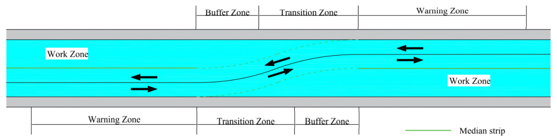
The spatial structure and traffic organization of the section are shown in Figure 1. Through the temporary opening, traffic is transferred between different carriageways. As a result, vehicle trajectories and speed variation patterns differ from those observed on conventional straight freeway sections.

Referring to the functional zoning method in road construction traffic organization standards and considering the characteristics of vehicle trajectory changes, the study section is divided along the driving direction into four areas: the Warning Zone, Transition Zone, Buffer Zone, and Work Zone. The Warning Zone provides construction information and supports speed adjustment. The Transition Zone is where vehicle trajectories shift, and lanes gradually change. The Buffer Zone serves as a safety transition area before vehicles enter the Work Zone. The Work Zone is the area where reconstruction and expansion activities are conducted.

Field speed data were collected from a median crossover section in the case project with a “two-lane to one-lane” configuration. The survey was conducted during off-peak hours on a weekday under clear weather and dry pavement conditions. Speed measurement sections included 100 m upstream of the opening, the opening start point, the opening midpoint, and the opening end point. The measured 85th percentile speeds at these four sections were 86.00 km/h, 72.85 km/h, 48.00 km/h, and 63.90 km/h, respectively. These field speed data were used to describe the longitudinal speed variation pattern of vehicles passing through the median crossover sections and to provide supplementary speed validation for the subsequent VISSIM model. The main traffic flow parameters used as model inputs are presented in

Table 1. Traffic flow parameters of a freeway reconstruction and expansion section.

Parameter	Item	Value
Peak Hourly Flow (PHV)	-	1450 pcu/h
Vehicle Composition	Passenger Cars	75%
	Heavy Trucks	10%
	Other	15%
Measured 85th Percentile Speed	Basic Section	70–75 km/h
	Median crossover section Opening Midpoint	45–50 km/h

Note: pcu = passenger car unit.

.

In the subsequent safety evaluation, a safety conflict rate threshold of ≤0.05 incidents/vehicle·km is adopted as the reference benchmark. To comprehensively evaluate speed limit strategies for median crossover sections in freeway reconstruction and expansion, a simulation matrix containing nine core scenarios is designed, as shown in

Table 2. Simulation matrix of traffic scenarios for median crossover sections in freeway reconstruction and expansion.

Traffic Saturation (Volume-to-Capacity, V/C Ratio)	Capacity Bottleneck (Two-Lane Merging into One-Lane, Forced Merging): a1	Speed Bottleneck (Single-Lane Splitting into Two Lanes, Speed Fluctuations): a2	Geometric Bottleneck (Single-Lane S-Shaped Curve, Abrupt Geometric Change): a3
Low Saturation (0.3): b1	a1b1	a2b1	a3b1
Medium Saturation (0.6): b2	a1b2	a2b2	a3b2
High Saturation (0.9): b3	a1b3	a2b3	a3b3

.

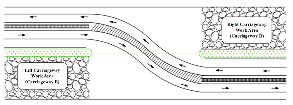
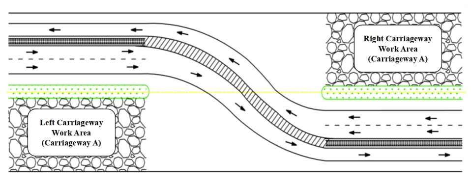
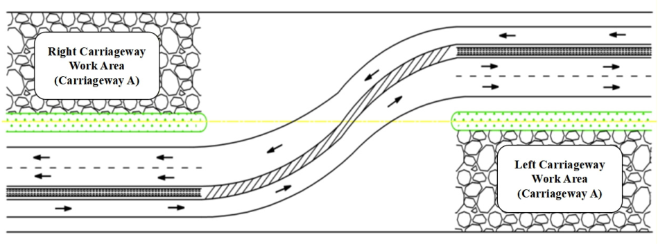
The three types of median crossover sections detailed in Table 2, representing different bottleneck characteristics—namely “capacity bottleneck,” “speed bottleneck,” and “geometric bottleneck”—are illustrated in Figure 2, Figure 3 and Figure 4.

Figure 2 shows a typical forced merging bottleneck, where traffic flow is forced to merge from two lanes into one lane. Figure 3 shows a section where traffic flow splits from one lane into two lanes. In this case, speed fluctuations and disturbances may occur because of uneven vehicle acceleration or differences in lane selection decisions. Figure 4 shows a section where vehicles remain in a single lane but must pass through an S-shaped curve with a small turning radius. This bottleneck is caused by an abrupt geometric change and may affect vehicle lateral stability and the speed adjustment process.

Based on the Chinese standard “Safety Work Rules for Highway Maintenance” (JTG H30-2015) [30], which recommends a gradual speed reduction of 10–20 km/h every 100–200 m, and the U.S. Manual on Uniform Traffic Control Devices for Streets and Highways (MUTCD 2009 Edition), which recommends no more than a 16 km/h speed reduction at a single step [31], this study adopts a baseline model of a 20 km/h reduction every 200 m.

Considering simulation equivalency, regulatory compliance, cost-effectiveness, and driver behavior, three-tiered speed limit schemes were designed for the median crossover section:

(1) Tiered Speed Limit Scheme One: A multi-stage speed reduction method (80→60→40 km/h), where the speed limit is set at 80 km/h before the warning zone, reduced to 60 km/h halfway through the warning zone, and further reduced to 40 km/h after 200 m, forming a stepped gradient speed reduction.

(2) Tiered Speed Limit Scheme Two: A single-stage speed reduction method (80→60 km/h), where the speed limit is set at 80 km/h before the warning zone, reduced to 60 km/h halfway through the warning zone, and maintained until the end of the speed limit zone.

(3) Tiered Speed Limit Scheme Three: A gradual speed reduction method (80→70 km/h), where the speed limit is set at 80 km/h before the warning zone, reduced to 70 km/h halfway through the warning zone, and maintained until the end of the speed limit zone.

By combining the three-tiered speed limit schemes with the simulation matrix shown in Table 2, a total of 27 simulation scenario combinations is formed for median crossover sections in freeway reconstruction and expansion. Each scenario is constructed based on the measured traffic flow parameters listed in Table 1.

It should be noted that the case in this study is used to represent a typical work zone scenario with median crossover sections characteristics. The proposed evaluation process can provide a reference for median crossover sections with similar geometric forms and traffic organization patterns. However, specific speed limits and scheme rankings should still be recalibrated and verified according to actual road conditions.

3.2. Construction of the Two-Stage Evaluation Process

3.2.1. Phase One: VISSIM Objective Simulation

(1) VISSIM Simulation Model Construction and Calibration

VISSIM has been widely demonstrated to be a reliable tool for microscopic traffic flow assessment. It can effectively quantify the impacts of various traffic control strategies on freeway operational efficiency and microscopic safety indicators [32]. In this study, a microscopic traffic simulation model was developed for the median crossover sections in a freeway reconstruction and expansion project. Referring to the Chinese standard Safety Work Rules for Highway Maintenance (JTG H30-2015), the length of the Warning Zone was set to 1600 m to provide drivers with sufficient distance for speed limit perception and deceleration response. The total length of the Transition Zone and Buffer Zone at the opening was set to 100 m, reflecting the continuous trajectory adjustment of vehicles within the crossover opening.

To improve model reproducibility, the simulation model was calibrated before its formal application. The calibration included desired speed settings, which were based on field speed survey data and the designed speed limit schemes, as well as driving behavior parameter calibration. Through sensitivity analysis, CC1, CC2, CC7, and CC8 were selected for orthogonal testing. The final calibrated parameters were CC1 = 1.00, CC2 = 5.00, CC7 = 0.60, and CC8 = 7.00. The detailed parameter settings are listed in

Table 3. Wiedemann 99 car-following parameters used in the calibrated VISSIM model.

Parameter	Meaning	Default Value	Simulation Value	Calibration Status
CC0	Standstill distance	1.50 m	1.50 m	Default value retained
CC1	Headway time	0.90 s	1.00 s	Calibrated value
CC2	Following variation	4.00 m	5.00 m	Calibrated value
CC3	Threshold for entering the following state	−8.00 s	−8.00 s	Default value retained
CC4	Negative following threshold	−0.35	−0.35	Default value retained
CC5	Positive following threshold	0.35	0.35	Default value retained
CC6	Speed oscillation	11.44	11.44	Default value retained
CC7	Oscillation acceleration	0.25 m/s2	0.60 m/s2	Calibrated value
CC8	Standstill acceleration	3.50 m/s2	7.00 m/s2	Calibrated value
CC9	Acceleration at 80 km/h	1.50 m/s2	1.50 m/s2	Default value retained

. Under this calibrated parameter combination, the simulated peak-hour traffic volume was 1428 pcu/h. Compared with the measured value of 1450 pcu/h, the relative error was 1.52%, indicating that the model can adequately reproduce the overall traffic flow level.

On the basis of traffic volume calibration, the 85th percentile speeds at key sections were further used to examine the model’s ability to reproduce the longitudinal speed variation pattern of vehicles. Based on the field speed data described in Section 3.1, four sections were selected: 100 m upstream of the opening, the opening start point, the opening midpoint, and the opening end point. The simulated 85th percentile speeds were compared with the measured values, as shown in

Table 4. Supplementary validation results for the 85th percentile speeds at key sections.

Section Location	Measured 85th Percentile Speed (km/h)	Simulated 85th Percentile Speed (km/h)	Relative Error
100 m upstream of the opening	86.00	83.35	3.08%
Opening start point	72.85	70.17	3.68%
Opening midpoint	48.00	45.97	4.23%
Opening end point	63.90	61.40	3.91%

. The relative errors at all four sections were less than 5%, indicating that the calibrated model can adequately reproduce both the representative speed levels at key sections and the longitudinal deceleration–recovery pattern.

For each combination of bottleneck type, traffic saturation level, and speed limit scheme, five random seeds were used for independent simulations. The average value was then adopted as the final evaluation data to reduce the influence of stochastic fluctuations.

The VISSIM simulation model outputs the following four indicators to quantify the comprehensive performance of each speed limit scheme:

Safety: As drivers navigate the median crossover section, they often engage in deceleration, lane changing, and other driving behaviors, which may increase the risk of rear-end collisions and other conflicts. Therefore, the vehicle conflict rate is used as the safety evaluation indicator. This rate is calculated through the interaction between VISSIM and the Surrogate Safety Assessment Model (SSAM), with a benchmark set at ≤0.05 incidents/vehicle·km based on field measurements.

Stability: Driving through the median crossover section, especially at the opening, involves a process of deceleration followed by acceleration. The smaller the speed variation, the more stable the driving conditions. To represent the stability of vehicle operation, the speed difference at three sections—beginning, middle, and end—of the opening is used, referred to as the two-section speed difference.

Traffic Efficiency: Delay refers to the time lost by drivers due to uncontrollable or unexpected disturbances while passing through the median crossover section, as well as the influence of traffic control measures. The smaller the delay, the less time is lost during the journey, leading to higher traffic efficiency. Thus, the average delay is selected as the evaluation indicator for traffic efficiency.

Fuel Economy: Fuel economy is a crucial factor for drivers when selecting their driving speed. In the absence of constraints like traffic flow or time, drivers typically choose an “economical speed.” Fuel economy is represented by fuel consumption per kilometer, which serves as the indicator for the fuel efficiency of vehicle operation.

(2) EWM-TOPSIS Method for Objective Evaluation

Based on the four indicators described above, the Technique for Order Preference by Similarity to an Ideal Solution (TOPSIS) method was introduced to systematically evaluate the comprehensive performance of each speed limit scheme. TOPSIS is a classical multi-criteria decision-making (MCDM) method. It ranks alternatives by calculating their relative distances from the positive ideal solution, where all indicators are optimal, and the negative ideal solution, where all indicators are the worst [33].

In MCDM, determining indicator weights is essential. This study adopts the Entropy Weight Method (EWM) to assign objective weights [34]. EWM is based on information theory. Its core principle is that an indicator with greater variation across alternatives, and thus lower information entropy, contains more useful information and should be assigned a higher weight. The calculation procedure of the EWM–TOPSIS method is as follows [33,34,35,36]:

① Indicator Normalization: Let $X_{ij}$ represent the original simulation result for the i-th speed limit scheme under the j-th evaluation indicator. Since each evaluation indicator has different units, the original simulation values are first normalized. Based on the nature of the indicators, they are categorized into benefit-type indicators (where larger values represent better operational performance) and cost-type indicators (where smaller values represent better operational status). The extreme value normalization method is applied to map each indicator to the range [0, 1], ensuring that traffic indicators with different physical meanings can be compared within the same evaluation framework, as shown in Equation (1).

$${{\mathrm{X}}_{\mathrm{i}\mathrm{j}}}^{\prime }=\left\{\begin{array}{c}{\displaystyle \frac{{\mathrm{X}}_{\mathrm{i}\mathrm{j}}-\mathrm{m}\mathrm{i}\mathrm{n}\left\{{\mathrm{X}}_{1\mathrm{j}},\dots ,{\mathrm{X}}_{\mathrm{n}\mathrm{j}}\right\}}{\mathrm{m}\mathrm{a}\mathrm{x}\left\{{\mathrm{X}}_{1\mathrm{j}},\dots ,{\mathrm{X}}_{\mathrm{n}\mathrm{j}}\right\}-\mathrm{m}\mathrm{i}\mathrm{n}\left\{{\mathrm{X}}_{1\mathrm{j}},\dots ,{\mathrm{X}}_{\mathrm{n}\mathrm{j}}\right\}}}\left(\mathrm{b}\mathrm{e}\mathrm{n}\mathrm{e}\mathrm{f}\mathrm{i}\mathrm{t}\text{-}\mathrm{t}\mathrm{y}\mathrm{p}\mathrm{e}\right)\\ {\displaystyle \frac{\mathrm{m}\mathrm{a}\mathrm{x}\left\{{\mathrm{X}}_{1\mathrm{j}},\dots ,{\mathrm{X}}_{\mathrm{n}\mathrm{j}}\right\}-{\mathrm{X}}_{\mathrm{i}\mathrm{j}}}{\mathrm{m}\mathrm{a}\mathrm{x}\left\{{\mathrm{X}}_{1\mathrm{j}},\dots ,{\mathrm{X}}_{\mathrm{n}\mathrm{j}}\right\}-\mathrm{m}\mathrm{i}\mathrm{n}\left\{{\mathrm{X}}_{1\mathrm{j}},\dots ,{\mathrm{X}}_{\mathrm{n}\mathrm{j}}\right\}}}\left(\mathrm{c}\mathrm{o}\mathrm{s}\mathrm{t}\text{-}\mathrm{t}\mathrm{y}\mathrm{p}\mathrm{e}\right)\end{array}\right.$$

(1)

In this study, the conflict rate, two-section speed difference, delay, and fuel consumption per kilometer are considered cost-type indicators.

Next, calculate the information entropy $E_j$ for the j-th indicator. First, compute the weight $P_{ij}$ for the i-th scheme, then calculate $E_j$ as shown in Equations (2) and (3).

$${\mathrm{P}}_{\mathrm{i}\mathrm{j}}={\displaystyle \frac{{{\mathrm{X}}_{\mathrm{i}\mathrm{j}}}^{\prime }}{{\sum }_{\mathrm{i}=1}^{\mathrm{n}}{{\mathrm{X}}_{\mathrm{i}\mathrm{j}}}^{\prime }}}$$

(2)

$${\mathrm{E}}_{\mathrm{j}}=-\mathrm{k}{\sum }_{\mathrm{i}=1}^{\mathrm{n}}{\mathrm{P}}_{\mathrm{i}\mathrm{j}}\ln \left({\mathrm{P}}_{\mathrm{i}\mathrm{j}}\right),\mathrm{k}={\displaystyle \frac{1}{\ln \mathrm{n}}}$$

(3)

where n = 3 represents the three-tiered speed limit schemes involved in the evaluation. $P_{ij}$ reflects the proportion of the performance of the speed limit strategy in a single dimension, such as safety or efficiency, after eliminating the influence of the units.

Finally, the final objective weight $W_j$ is calculated using the information entropy redundancy $D_j=1-E_j$, as shown in Equation (4).

$${\mathrm{W}}_{\mathrm{j}}={\displaystyle \frac{{\mathrm{D}}_{\mathrm{j}}}{{\sum }_{\mathrm{j}=1}^{\mathrm{m}}{\mathrm{D}}_{\mathrm{j}}}}={\displaystyle \frac{1-{\mathrm{E}}_{\mathrm{j}}}{{\sum }_{\mathrm{j}=1}^{\mathrm{m}}\left(1-{\mathrm{E}}_{\mathrm{j}}\right)}}$$

(4)

where m = 4 represents the four indicators involved in the evaluation.

This step achieves the automatic focus of the evaluation criteria, meaning that the weights $W_j$ will automatically shift towards those indicators that can significantly distinguish the performance differences among the speed limit schemes, thereby ensuring the objectivity of the first-phase evaluation.

② Construct the Weighted Matrix $Z$: Based on the normalized matrix ${X_{ij}}^{\prime }$ and the objective weights $W_j$, the weighted normalized matrix $Z$ is constructed, as shown in Equation (5).

$${\mathrm{Z}}_{\mathrm{j}}={\mathrm{W}}_{\mathrm{j}}\times {{\mathrm{X}}_{\mathrm{i}\mathrm{j}}}^{\prime }$$

(5)

③ Determine the Ideal Solution $Z^{+}$ and the Negative Ideal Solution $Z^{-}$: Based on the weighted matrix $Z$, the “ideal solution” $Z^{+}$ (the optimal value for each indicator) and the “negative ideal solution” $Z^{-}$ (the worst value for each indicator) are determined. In this study, $Z^{+}$ represents the ideal reference solution where the speed limit scheme achieves optimal performance in terms of safety, operational efficiency, and stability under the current traffic scenario and bottleneck conditions. $Z^{-}$ represents the extreme scenario with the worst possible comprehensive operational performance, as shown in Equations (6) and (7):

$${\mathrm{Z}}^{+}=\left({{\mathrm{Z}}_1}^{+},{{\mathrm{Z}}_2}^{+},\dots ,{{\mathrm{Z}}_{\mathrm{m}}}^{+}\right)=\left(\mathrm{m}\mathrm{a}\mathrm{x}{\mathrm{Z}}_{\mathrm{i}1},\mathrm{m}\mathrm{a}\mathrm{x}{\mathrm{Z}}_{\mathrm{i}2},\dots ,\mathrm{m}\mathrm{a}\mathrm{x}{\mathrm{Z}}_{\mathrm{i}\mathrm{m}}\right)$$

(6)

$${\mathrm{Z}}^{-}=\left({{\mathrm{Z}}_1}^{-},{{\mathrm{Z}}_2}^{-},\dots ,{{\mathrm{Z}}_{\mathrm{m}}}^{-}\right)=\left(\mathrm{m}\mathrm{i}\mathrm{n}{\mathrm{Z}}_{\mathrm{i}1},\mathrm{m}\mathrm{i}\mathrm{n}{\mathrm{Z}}_{\mathrm{i}2},\dots ,\mathrm{m}\mathrm{i}\mathrm{n}{\mathrm{Z}}_{\mathrm{i}\mathrm{m}}\right)$$

(7)

④ Calculate the Distances ${D_i}^{+}$ and ${D_i}^{-}$: The Euclidean distance is used to measure the deviation of the i-th speed limit scheme from the ideal solution and the negative ideal solution, as shown in Equations (8) and (9):

$${{\mathrm{D}}_{\mathrm{i}}}^{+}=\sqrt{{\sum }_{\mathrm{i}=1}^{\mathrm{m}}{(\mathrm{m}\mathrm{a}\mathrm{x}{\mathrm{Z}}_{\mathrm{i}\mathrm{j}}-{\mathrm{Z}}_{\mathrm{i}\mathrm{j}})}^2}$$

(8)

$${{\mathrm{D}}_{\mathrm{i}}}^{-}=\sqrt{{\sum }_{\mathrm{i}=1}^{\mathrm{m}}{(\mathrm{m}\mathrm{i}\mathrm{n}{\mathrm{Z}}_{\mathrm{i}\mathrm{j}}-{\mathrm{Z}}_{\mathrm{i}\mathrm{j}})}^2}$$

(9)

⑤ Calculate the Relative Closeness $C_i$ to the Ideal Solution: Typically, $0\ll C_i\ll 1$, where a value closer to 1 indicates better overall performance of the scheme. In this study, $C_i$ is used as the final output of the first-phase VISSIM objective simulation evaluation to assess the objective technical superiority or inferiority of different speed limit schemes across various traffic scenarios, providing quantitative data for the subsequent FAHP multi-objective decision-making process, as shown in Equation (10):

$${\mathrm{C}}_{\mathrm{i}}={\displaystyle \frac{{{\mathrm{D}}_{\mathrm{i}}}^{-}}{{{\mathrm{D}}_{\mathrm{i}}}^{+}+{{\mathrm{D}}_{\mathrm{i}}}^{-}}}$$

(10)

3.2.2. Phase Two: FAHP Multi-Criteria Evaluation

(1) Construction of the FAHP Evaluation System

The core of the FAHP is to decompose a complex decision-making problem into a multi-level hierarchical structure consisting of the goal, criteria, and indicators. By introducing triangular fuzzy numbers, FAHP can effectively address the fuzziness and uncertainty inherent in expert judgments, thereby establishing a multi-level comprehensive evaluation model [37,38].

Based on the literature review in Section 2 on work zone speed control, economic and environmental impacts, simulation-based evaluation, and multi-criteria decision-making, and considering the operating characteristics of median crossover sections and the results of expert consultation, this study establishes a speed limit scheme evaluation system comprising six criteria layers (B) and 21 indicator layers (C). This system includes evaluation dimensions that can be supported by simulation outputs or engineering data, such as safety, efficiency, and environment. It also incorporates decision-making factors that are difficult to directly capture through microscopic traffic simulation, including economic, driving psychology, and social policy considerations. The specific indicator system is presented in

Table 5. Evaluation system for speed limit indicators of median crossover sections in freeway reconstruction and expansion.

Criteria Layer (B)	Indicator Layer (C)	Explanation
B1: Safety	C1: Horizontal Curve Radius	Key geometric parameter affecting vehicle lateral stability
	C2: Longitudinal Slope	Affects vehicle acceleration and deceleration safety
	C3: Sight Distance	Affects driver’s visibility and reaction time
	C4: Traffic Volume (V/C Ratio)	High traffic volume increases conflict risks
	C5: Truck Proportion	Trucks affect speed differences, increasing lane change conflict risks
	C6: Speed Dispersion	Large speed differences increase the risk of rear-end collisions and other accidents
	C7: Historical Accident Rate	Reflects the operational safety risks of the section
B2: Efficiency	C8: Average Travel Speed	Reflects the impact of speed limits on traffic efficiency
	C9: Peak Hour Delay Rate	Adaptability of speed limits under peak congestion
	C10: Traffic Capacity	The impact of speed limits on the section’s maximum traffic capacity
B3: Economic	C11: Reconstruction Cost	Costs of engineering modifications due to speed limit adjustments
	C12: Operation and Maintenance Costs	Long-term operational and maintenance costs
	C13: Economic Loss from Accidents	Economic losses due to accidents
B4: Environment	C14: Noise Level	Impact of speed limits on vehicle noise emissions
	C15: CO2 Emissions	Control of emissions under low-carbon traffic requirements
	C16: Fuel Consumption	Optimization of fuel efficiency under economical speeds
B5: Driver Psychology	C17: Driver Psychological Load	Matching speed limits with the driver’s psychological tolerance
	C18: Speed Compliance Rate	Reflects driver adherence to speed limits
	C19: Driver Satisfaction	User acceptance of the speed limit scheme
B6: Social Policy	C20: Public Acceptance	Social opinion regarding the acceptability of the speed limit scheme
	C21: Policy and Regulatory Compliance	Conformance with traffic management policies and regulations

.

(2) Expert Survey and Judgment Matrix Construction

To obtain expert judgment information for the multi-criteria evaluation of speed limit schemes, 15 experts in the field of traffic engineering were invited to participate in the FAHP fuzzy judgment scoring. All members of the expert panel held senior professional titles or above. Their expertise covered five professional fields: freeway survey and design, freeway construction management, freeway operation management, traffic safety and traffic simulation research, and traffic policy, standards, and specifications. The composition of the expert panel is shown in

Table 6. Composition of the FAHP expert panel.

Expert Category	Number of Experts	Professional Background
Freeway survey and design	3	Freeway survey and design, reconstruction and expansion engineering design, traffic organization design
Freeway construction management	3	Reconstruction and expansion construction organization, work zone layout, traffic maintenance during construction
Freeway operation management	3	Freeway operation control, traffic organization, operational safety management
Traffic safety and simulation research	3	Traffic safety evaluation, microscopic traffic simulation, speed limit strategy analysis
Traffic policy and technical standards	3	Traffic management policy, highway engineering standards and specifications, work zone management requirements
Total	15	—

.

The expert survey consisted of two parts: the criteria layer and the indicator layer. The criteria layer included six evaluation criteria: safety, operational efficiency, economic cost, energy and environment, driving behavior and psychology, and social and policy considerations. The indicator layer included the corresponding sub-indicators under each criterion. Based on the triangular fuzzy number (TFN)-based Saaty 1–9 scale, the experts independently conducted pairwise comparisons of the relative importance of indicators within the same layer. The correspondence between the fuzzy scale and triangular fuzzy numbers is presented in

Table 7. Fuzzy Scale and Triangular Fuzzy Number Correspondence.

Saaty Scale (Language Description)	Value	Fuzzy Number
Equally Important (EI)	1	(1, 1, 1)
Slightly Important (SI)	3	(2, 3, 4)
Quite Important (QI)	5	(4, 5, 6)
Very Important (VI)	7	(6, 7, 8)
Absolutely Important (AI)	9	(8, 9, 10)
Intermediate Value Between Two Adjacent Scales	2	(1, 2, 3)
	4	(3, 4, 5)
	6	(5, 6, 7)
	8	(7, 8, 9)

.

(3) Aggregation of Expert Judgments, Weight Calculation, and Consistency Check

Let the triangular fuzzy judgment of the k-th expert for indicator i relative to indicator j be denoted as ${\tilde{a}}_{ij}^{\left(k\right)}=(l_{ij}^{\left(k\right)},m_{ij}^{\left(k\right)},u_{ij}^{\left(k\right)})$, where l, m, and u represent the lower bound, most likely value, and upper bound of the triangular fuzzy number, respectively. For the same indicator pair, this study adopts the arithmetic mean method to aggregate the judgments of the 15 experts and obtain the integrated fuzzy judgment value, as shown in Equation (11):

$${\tilde{\mathrm{a}}}_{\mathrm{i}\mathrm{j}}=\left({\displaystyle \frac{1}{\mathrm{K}}}{\displaystyle \sum _{\mathrm{k}=1}^{\mathrm{K}}}{\mathrm{l}}_{\mathrm{i}\mathrm{j}}^{\left(\mathrm{k}\right)},{\displaystyle \frac{1}{\mathrm{K}}}{\displaystyle \sum _{\mathrm{k}=1}^{\mathrm{K}}}{\mathrm{m}}_{\mathrm{i}\mathrm{j}}^{\left(\mathrm{k}\right)},{\displaystyle \frac{1}{\mathrm{K}}}{\displaystyle \sum _{\mathrm{k}=1}^{\mathrm{K}}}{\mathrm{u}}_{\mathrm{i}\mathrm{j}}^{\left(\mathrm{k}\right)}\right)$$

(11)

where K is the number of experts. This aggregation procedure forms the integrated fuzzy judgment matrix and reduces the influence of any single expert’s judgment on the aggregated results.

After the integrated fuzzy judgment matrix is obtained, consistency checks are first conducted for the judgment matrices at each layer. For an n-order judgment matrix, the consistency index (CI) and consistency ratio (CR) are calculated using Equations (12) and (13), respectively:

$$\mathrm{C}\mathrm{I}={\displaystyle \frac{{\mathsf{\lambda }}_{\mathrm{m}\mathrm{a}\mathrm{x}}-\mathrm{n}}{\mathrm{n}-1}}$$

(12)

$$\mathrm{C}\mathrm{R}={\displaystyle \frac{\mathrm{C}\mathrm{I}}{\mathrm{R}\mathrm{I}}}$$

(13)

where ${\lambda }_{\mathrm{m}\mathrm{a}\mathrm{x}}$ is the maximum eigenvalue of the judgment matrix, and RI is the random consistency index. When CR < 0.1, the judgment matrix is considered to have acceptable consistency.

After passing the consistency check, the geometric mean method is used to calculate the triangular fuzzy weights of each indicator [39]. The centroid method is then applied to transform the triangular fuzzy weights into crisp values [40], as shown in Equation (14):

$$W_{clear}={\displaystyle \frac{l+4m+u}{6}}$$

(14)

The defuzzified weights are subsequently normalized to obtain the weights of the criteria layer and indicator layer. The consistency check results for the judgment matrices at each layer are presented in

Table 8. Consistency check results of the FAHP judgment matrices.

Judgment Matrix	Matrix Dimension	Consistency Ratio (CR)	Consistency Check Result
Criteria layer B1–B6	6 × 6	0.0415	Passed
Safety indicator layer C1–C7	7 × 7	0.0809	Passed
Efficiency indicator layer C8–C10	3 × 3	0.0462	Passed
Economic indicator layer C11–C13	3 × 3	0.0462	Passed
Environment indicator layer C14–C16	3 × 3	0.0462	Passed
Driving psychology indicator layer C17–C19	3 × 3	0.0462	Passed
Social policy indicator layer C20–C21	2 × 2	0.0000	Passed

. The results show that the CR values of all judgment matrices are less than 0.1, indicating that they are suitable for subsequent FAHP weight calculation.

It should be noted that the social policy indicator layer C20–C21 is a 2 × 2 judgment matrix, which naturally satisfies the consistency requirement. Therefore, its CR value is 0.0000.

(4) Comprehensive Score Calculation

Each scheme is evaluated by experts across 21 sub-indicators using a five-level discrete rating system, $\mathrm{V}=\left\{\mathrm{E}\mathrm{x}\mathrm{c}\mathrm{e}\mathrm{l}\mathrm{l}\mathrm{e}\mathrm{n}\mathrm{t},\mathrm{G}\mathrm{o}\mathrm{o}\mathrm{d},\mathrm{F}\mathrm{a}\mathrm{i}\mathrm{r},\mathrm{P}\mathrm{o}\mathrm{o}\mathrm{r},\mathrm{Very}\mathrm{Poor}\right\}=\left\{5,4,3,2,1\right\}$. A two-layer weighted summation model is applied to compute the final comprehensive score [41].

First, the score of each criterion layer $S_{B_i}$ is calculated as the weighted sum of its corresponding sub-indicators, as expressed in Equation (15):

$$S_{B_i}={\sum }_{j=1}^{m_i}\left(S_{C_{i,j}}\times W_{C_{i,j}}\right)$$

(15)

where

$S_{B_i}$ is the comprehensive score of the i-th criterion;

$S_{C_{i,j}}$ is the average expert rating of the j-th indicator under the i-th criterion;

$W_{C_{i,j}}$ is the normalized weight of the j-th indicator under the i-th criterion;

$m_i$ is the number of indicators under the i-th criterion.

Subsequently, the overall comprehensive score of the scheme, $S_{total}$ is calculated as the weighted sum of all criterion-layer scores, as shown in Equation (16):

$$S_{total}={\sum }_{i=1}^6\left(S_{B_i}\times W_{B_i}\right)$$

(16)

where

$W_{B_i}$ is the normalized weight of the i-th criterion;

$S_{total}$ is the global comprehensive score of the scheme.

(5) Sensitivity Analysis

Sensitivity analysis is conducted by perturbing the weights of the six primary criteria (B1–B6) by ±10% and recalculating the overall comprehensive score. The resulting changes in scheme rankings are then examined to determine whether variations in criterion weights lead to significant shifts in decision outcomes. This procedure evaluates the stability and robustness of the proposed decision-making model [42].

3.2.3. Two-Stage Evaluation Process

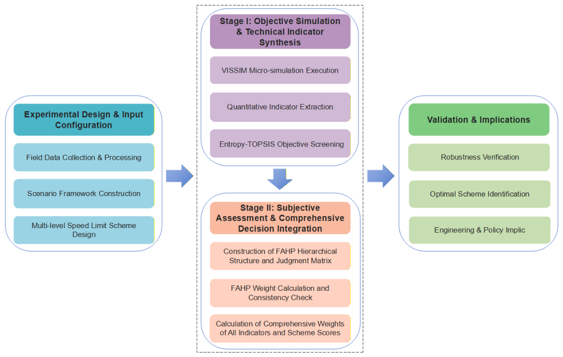
Based on the Phase One VISSIM objective simulation and the Phase Two FAHP subjective evaluation, this study develops a two-stage evaluation process for speed limit strategies at median crossover sections in freeway reconstruction and expansion, as shown in Figure 5.

As shown in Figure 5, the evaluation of speed limit strategies for median crossover sections in freeway reconstruction and expansion begins with the design of road section types characterized by different bottleneck features. VISSIM is then used to simulate the tiered speed limit schemes for each road section type under low, medium, and high traffic saturation levels. The EWM–TOPSIS method is subsequently applied to obtain the objective technical ranking of each scheme. In the second stage, a multi-objective evaluation system is established for speed limit schemes at median crossover sections. This system includes six primary criteria—safety, efficiency, economic cost, environment, driving psychology, and policy—together with 21 indicators. The FAHP method is then used to integrate objective microscopic traffic simulation data with expert-assessed qualitative decision factors, thereby producing a comprehensive evaluation of the speed limit schemes.

4. Results

4.1. Phase One: VISSIM Objective Simulation Results

4.1.1. Analysis of VISSIM Simulation Outputs

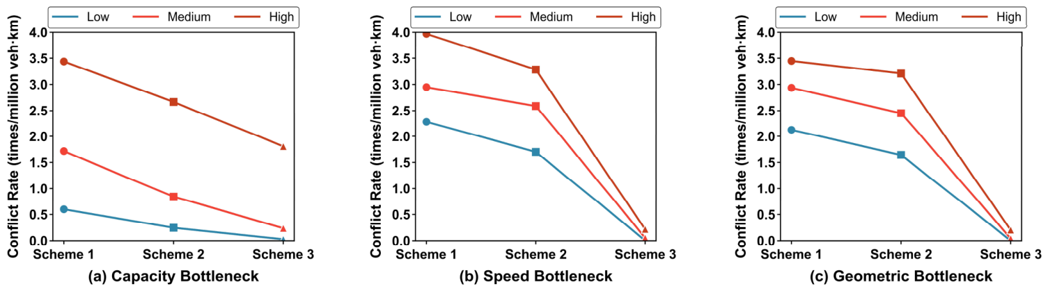
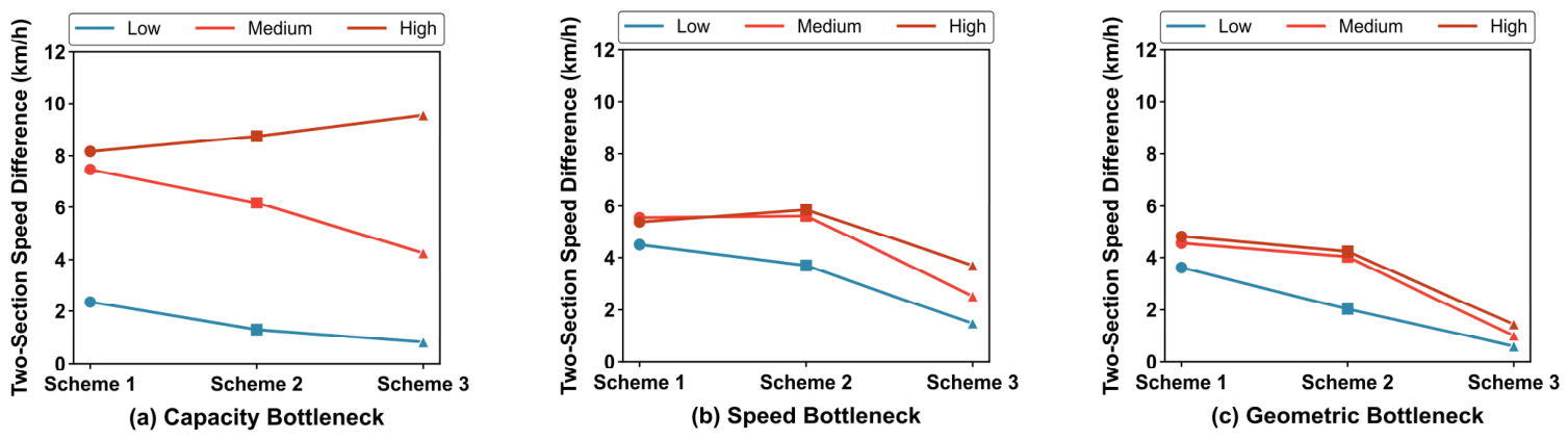
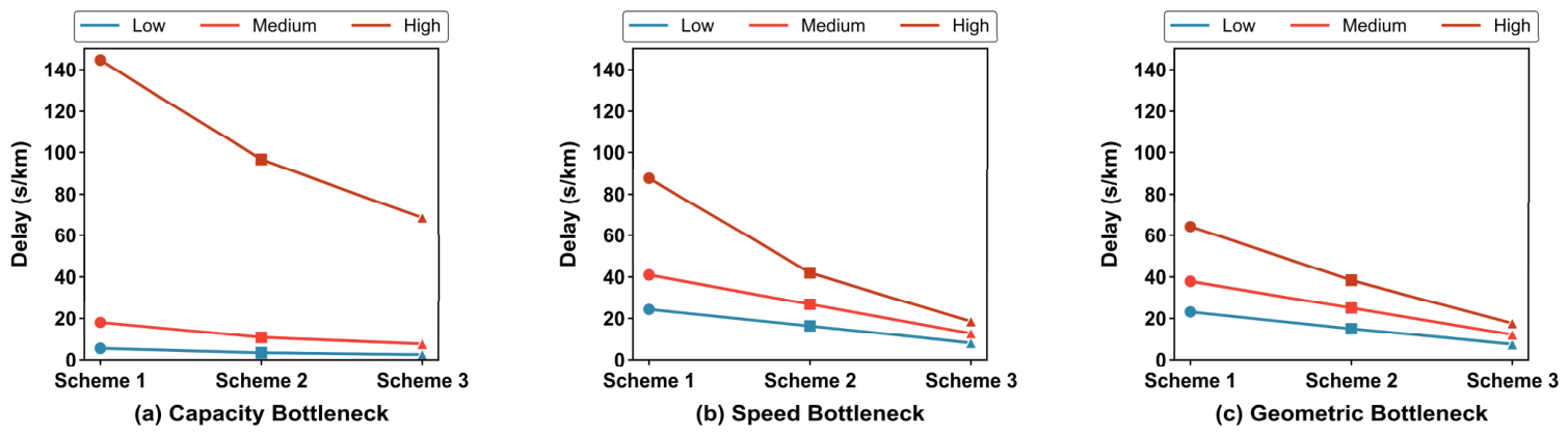
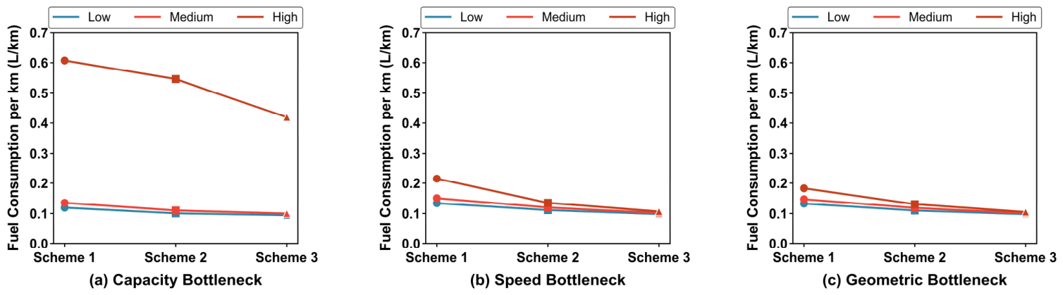
VISSIM was used to simulate traffic operations at median crossover sections in freeway reconstruction and expansion under three road section types and three speed limit schemes. The vehicle conflict rate, two-section speed difference, average delay, and fuel consumption per kilometer under low, medium, and high saturation levels are shown in Figure 6, Figure 7, Figure 8 and Figure 9.

As shown in Figure 6, Figure 8 and Figure 9, the speed limit schemes differ in conflict rate, average delay, and fuel consumption per kilometer across different combinations of bottleneck types and traffic saturation levels. In most scenarios, Scheme 3 (80→70 km/h) produces lower values for these indicators than Scheme 1 (80→60→40 km/h) and Scheme 2 (80→60 km/h).

Figure 7 shows that the schemes do not exhibit fully consistent performance in terms of the two-section speed difference. In particular, under the high-saturation capacity bottleneck scenario, where two lanes are forced to merge into one, and the V/C ratio is 0.9, the two-section speed difference in Scheme 3 is higher than that of Scheme 1. Overall, the VISSIM outputs reveal differences among the speed limit schemes in safety, speed stability, traffic efficiency, and fuel economy. These results provide the basic data for the subsequent multi-indicator comprehensive evaluation using the EWM–TOPSIS method.

4.1.2. Objective Comprehensive Evaluation Based on EWM–TOPSIS

To further compare the technical performance of different speed limit schemes across all simulation scenarios, the EWM–TOPSIS method was used to conduct a comprehensive evaluation based on four microscopic simulation indicators: conflict rate, two-section speed difference, average delay, and fuel consumption per kilometer. All four indicators are cost-type indicators, meaning that lower values indicate better scheme performance. After the objective weights of the indicators were determined using the Entropy Weight Method, the relative closeness $C_i$ between each of the three speed limit schemes and the positive ideal solution was calculated. A $C_i$ value closer to 1 indicates that the scheme is closer to the comprehensive optimal state. The relative closeness values of the speed limit schemes under the three bottleneck scenarios are presented in

Table 9. EWM–TOPSIS relative closeness values of speed limit schemes under the three bottleneck conditions.

Bottleneck Type	Saturation Level	Scheme 1	Scheme 2	Scheme 3
Capacity bottleneck	Low	0.000000	0.687391	1.000000
Capacity bottleneck	Medium	0.000000	0.579126	1.000000
Capacity bottleneck	High	0.344985	0.480106	0.655015
Speed bottleneck	Low	0.000000	0.379514	1.000000
Speed bottleneck	Medium	0.013892	0.230288	1.000000
Speed bottleneck	High	0.120237	0.338607	1.000000
Geometric bottleneck	Low	0.000000	0.437979	1.000000
Geometric bottleneck	Medium	0.000000	0.304235	1.000000
Geometric bottleneck	High	0.000000	0.285368	1.000000

.

As shown in Table 9, Scheme 3 (80→70 km/h) achieves the highest relative closeness across all combinations of the three bottleneck types and three traffic saturation levels. Under the speed bottleneck and geometric bottleneck scenarios, the relative closeness of Scheme 3 is 1.000000 under low, medium, and high saturation levels. Under the capacity bottleneck scenario, Scheme 3 also reaches 1.000000 under low and medium saturation levels. Although its relative closeness decreases to 0.655015 under high saturation, it remains higher than those of Scheme 1 and Scheme 2.

Scheme 1 (80→60→40 km/h) shows relatively low closeness values in most scenarios, especially under low and medium saturation levels, where its values are repeatedly zero or close to zero. Scheme 2 (80→60 km/h) generally falls between Scheme 1 and Scheme 3 in terms of relative closeness. These results indicate that, under the comprehensive evaluation of the four technical indicators used in this study, Scheme 3 maintains the highest objective ranking across all three bottleneck conditions. At the same time, the relative closeness gap among the schemes narrows under the high-saturation capacity bottleneck scenario. This result provides an objective simulation basis for the subsequent FAHP multi-criteria evaluation.

4.2. Phase Two: FAHP Multi-Criteria Evaluation Results

4.2.1. FAHP Weight Analysis

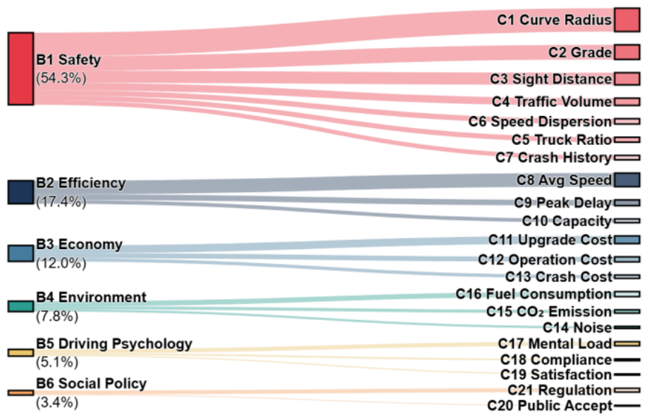
After the aggregation of expert judgment matrices, consistency checks, and weight calculation, the FAHP weights of the criteria layer and indicator layer were obtained. Figure 10 presents the global weight distribution of the six criteria and their corresponding 21 indicators.

As shown in Figure 10, Safety (B1) has the highest normalized weight in the criteria layer, accounting for 54.3%. It is followed by Efficiency (B2) and Economic (B3), with weights of 17.4% and 12.0%, respectively. The weights of Environment (B4), Driving Psychology (B5), and Social Policy Considerations (B6) are 7.8%, 5.1%, and 3.4%, respectively. These results indicate that safety is the most important criterion in the FAHP evaluation system established in this study, while operational efficiency and economic cost also play important roles in the comprehensive evaluation.

At the indicator layer, Horizontal Curve Radius (C1), Longitudinal Slope (C2), and Sight Distance (C3) under the Safety criterion have relatively high weights. This suggests that geometric conditions and sight distance are important factors in the safety evaluation of median crossover sections. Under the Operational Efficiency criterion, the weight of Average Travel Speed (C8) is higher than that of Peak Hour Delay Rate (C9) and Traffic Capacity (C10). Under the Energy and Environment criterion, Fuel Consumption (C16) has a relatively high weight. Under the Driving Behavior and Psychology criterion, Driver Psychological Load (C17) receives a relatively high weight. Under the Social and Policy Considerations criterion, Policy and Regulatory Compliance (C21) has a higher weight than Public Acceptance (C20).

Overall, the FAHP weight results indicate that the evaluation of speed limit schemes for median crossover sections primarily emphasizes safety, while also considering operational efficiency, economic cost, energy and environment, driving behavior, and policy adaptability. These weight results provide the criteria-layer and indicator-layer basis for calculating the comprehensive scores of different speed limit schemes in the subsequent analysis.

4.2.2. FAHP Comprehensive Scores of the Schemes

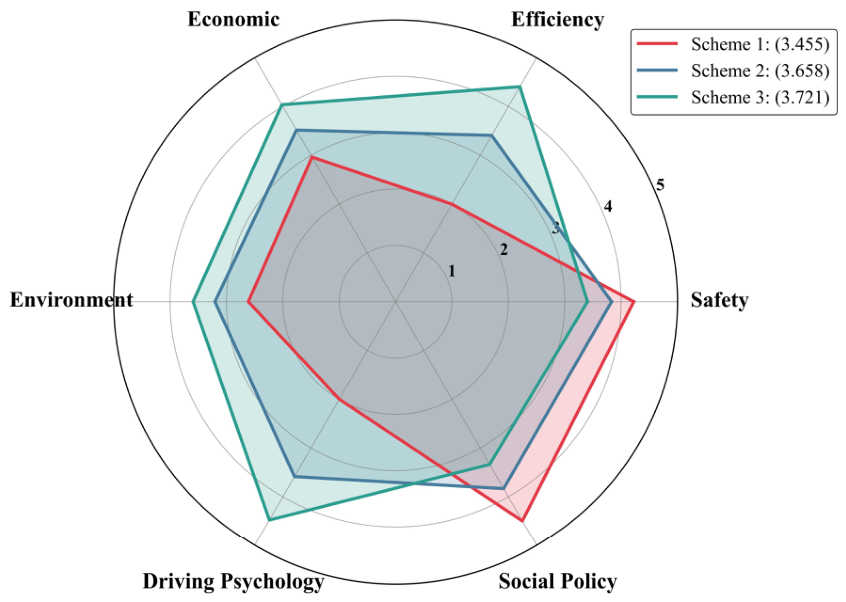
Based on expert ratings and FAHP weights, the scores of the three speed-limit schemes under the six criteria and their comprehensive scores were calculated using Equations (15) and (16). The criteria weights and comprehensive evaluation results are presented in

Table 10. Criterion-level scores and comprehensive evaluation results based on FAHP.

Item	Safety B1	Efficiency B2	Economic B3	Environment B4	Driver Psychology B5	Social Policy B6	Comprehensive Score
Weight ($W_{B_i}$)	0.543	0.174	0.120	0.078	0.051	0.034	—
Scheme 1	4.224	1.998	2.964	2.612	1.998	4.496	3.455
Scheme 2	3.831	3.408	3.518	3.204	3.585	3.832	3.658
Scheme 3	3.404	4.407	4.036	3.592	4.476	3.336	3.721

Note: The first row shows the criteria weights $W_{B_i}$, and the values in the scheme rows represent the criterion-level scores $S_{B_i}$ of each scheme under the corresponding criterion.

, and Figure 11 shows the score distribution of each scheme across the six criteria.

As shown in Table 10 and Figure 11, the three speed limit schemes perform differently across the criteria dimensions. Scheme 1 obtains relatively high scores for Safety (B1) and Social Policy Considerations (B6), but lower scores for Efficiency (B2), Environment (B4), and Driving Psychology (B5). The scores of Scheme 2 generally fall between those of Scheme 1 and Scheme 3 across the criteria. Scheme 3 achieves higher scores for Efficiency (B2), Economic (B3), Environment (B4), and Driving Psychology (B5). Its comprehensive score is therefore higher than those of Scheme 1 and Scheme 2.

The comprehensive scores of Scheme 1, Scheme 2, and Scheme 3 are 3.455, 3.658, and 3.721, respectively, resulting in the ranking Scheme 3 > Scheme 2 > Scheme 1. The FAHP comprehensive score ranking is broadly consistent with the objective ranking obtained from EWM–TOPSIS. This indicates that Scheme 3 has relatively strong comprehensive performance within the evaluation system established in this study.

4.2.3. Sensitivity Analysis

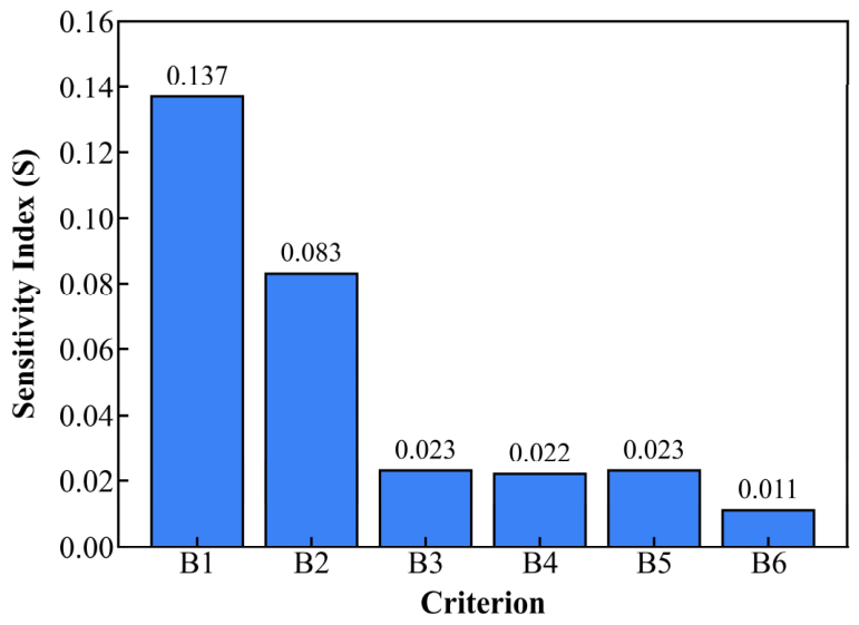
To examine the sensitivity of the FAHP multi-criteria evaluation results to changes in criteria-layer weights, a ±10% perturbation was applied separately to the weights of the six primary criteria (B1–B6). The perturbed weights were then normalized, and the comprehensive scores of the three speed-limit schemes were recalculated. In this study, the sensitivity index S is defined as the sum of the absolute changes in the comprehensive scores of all schemes under a ±10% perturbation of a given criterion weight. A larger S value indicates a stronger influence of the corresponding criterion weight on the comprehensive evaluation results. Figure 12 presents the sensitivity indices of the six primary criteria.

As shown in Figure 12, Safety (B1) has the highest sensitivity index, with S = 0.137, followed by Efficiency (B2), with S = 0.083. The sensitivity indices of Economic (B3), Environment (B4), and Driver Psychology (B5) are 0.023, 0.022, and 0.023, respectively, while Social Policy (B6) has the lowest sensitivity index, with S = 0.011. These results indicate that, within the ±10% weight perturbation range, changes in the weights of Safety and Efficiency have relatively greater effects on the comprehensive scores, whereas perturbations in the remaining criteria weights have relatively smaller effects.

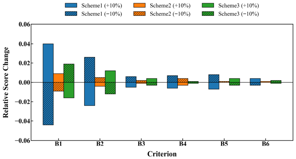
To further compare the score variations in the three speed limit schemes under weight perturbations, the relative changes in the comprehensive score of each scheme were calculated under ±10% perturbations of the six criteria. The results are shown in Figure 13.

As shown in Figure 13, the three speed-limit schemes respond differently to perturbations in different criteria weights. Score variations are relatively more evident under perturbations of Safety B1 and Efficiency B2. Specifically, Scheme 1 is more sensitive to perturbations in B1, whereas Scheme 2 is more sensitive to perturbations in B2. Scheme 3 shows relatively small score variations under all perturbation conditions. Across all 12 weight perturbation scenarios, the ranking of the three schemes remains unchanged as Scheme 3 > Scheme 2 > Scheme 1, indicating that the FAHP comprehensive evaluation results have a certain degree of stability within the ±10% weight perturbation range.

4.2.4. Comparison of Field Speed Characteristics

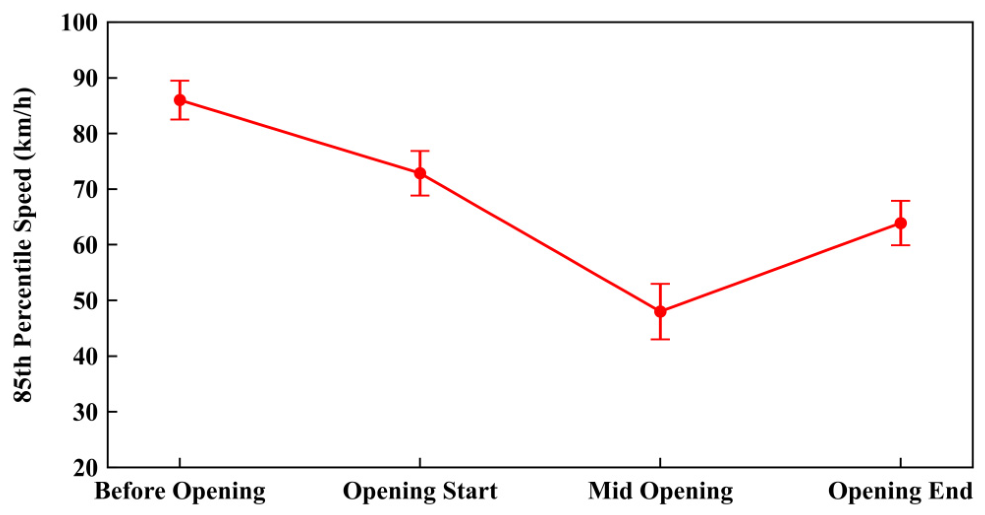
To further illustrate the longitudinal speed variation characteristics of vehicles passing through median crossover sections, the field speed data described above were used for an illustrative comparison. The variation in the measured 85th percentile speed is shown in Figure 14.

As shown in Figure 14, vehicles begin to decelerate before approaching the median crossover sections. The measured 85th percentile speed is 86.00 km/h at 100 m upstream of the opening and decreases to 72.85 km/h at the opening start point. After entering the opening, vehicles are affected by geometric changes and lateral trajectory shifts. As a result, the 85th percentile speed further decreases to 48.00 km/h at the opening midpoint. At the opening end point, the 85th percentile speed increases to 63.90 km/h. The error bars represent the standard error of the measured speed data.

These field data are used only to illustrate the longitudinal speed variation trend of vehicles passing through the crossover opening. They do not constitute external validation for all simulation scenarios.

5. Discussion and Limitations

5.1. Comprehensive Interpretation of the Speed Limit Scheme Evaluation Results

The results of this study show that the gradual speed reduction scheme (80→70 km/h) achieves a relatively high comprehensive performance in both the EWM–TOPSIS objective evaluation and the FAHP comprehensive evaluation. This finding is generally consistent with existing knowledge in work zone speed limit research regarding speed differences, speed dispersion, and vehicle operating stability. Previous studies have shown that abrupt geometric changes, restricted sight distance, and increased speed differences between vehicles can affect operational safety in work zones [6,8,9]. For median crossover sections in freeway reconstruction and expansion, the evaluation of speed limit schemes should not focus only on reducing absolute speed. It should also consider the continuity of the deceleration process, traffic flow stability, and driver adaptability to speed limit changes.

From the perspective of scheme comparison, Scheme 1 (80→60→40 km/h) sets a lower final speed limit, but it does not achieve better comprehensive evaluation results in most scenarios. Related studies on work zone speed control have also indicated that the safety benefits of reducing work zone speed are conditional. The actual effects are influenced by traffic conditions, work zone layout, and driver behavioral responses [15]. Combined with the results of this study, an excessive speed reduction may lead to uneven deceleration, car-following disturbances, and local queuing, thereby affecting traffic efficiency and fuel economy.

Driver response behavior also influences the effectiveness of speed limits. Existing studies have shown that the effectiveness of variable speed limit control is related to driver compliance behavior [14]. Single-objective optimization based solely on technical indicators may also overlook drivers’ psychological load and adaptability [16]. The field speed comparison in this study shows that vehicles begin to decelerate naturally before approaching the median crossover sections and reach a relatively low speed level near the midpoint of the opening. This trend is generally consistent with the design logic of the gradual speed reduction scheme and helps explain the relative advantage of Scheme 3 in the driving behavior and psychology dimension. However, the field speed data are mainly used to illustrate the speed variation characteristics of vehicles passing through the crossover opening. They cannot directly replace the validation of driver compliance with posted speed limits.

5.2. Differences in Bottleneck Types and the Mechanisms of Speed Limit Effects

The mechanisms through which speed limit schemes affect traffic operations differ across bottleneck types. In the capacity bottleneck scenario, traffic flow merges from two lanes into one lane, and vehicles must complete both merging and speed adjustment near the opening. Existing studies have shown that merging behavior in work zones is affected by factors such as lane closure type, traffic volume, vehicle type, and the availability of gaps in the target lane [43]. The risk of merging conflicts on freeways is also related to traffic flow conditions and driver decision-making environments [44]. Therefore, under high-saturation forced merging conditions, speed limit schemes affect not only speed levels but also speed coordination and local conflict risk during the merging process. In this study, the relative closeness gap among the schemes narrows under the high-saturation capacity bottleneck scenario. This indicates a more evident trade-off between speed, stability and traffic efficiency in this scenario. Lower operating speeds may reduce local speed differences, but they may also reduce capacity and induce queuing.

In the speed bottleneck scenario, vehicles split from one lane into two lanes. Differences in acceleration recovery and lane selection may affect local speed fluctuations. In the geometric bottleneck scenario, vehicles must pass through an S-shaped curve, where abrupt geometric changes impose higher requirements on lateral stability and speed control. In such scenarios, speed limit schemes should be matched with curve radius, sight distance, and vehicle lateral stability, rather than simply reducing the target speed. Overall, the three bottleneck scenarios indicate that speed limit design for median crossover sections should be comprehensively determined by considering bottleneck causes, traffic saturation levels, and vehicle operating trajectories.

5.3. Engineering Applicability and Sustainable Traffic Management

From the perspective of engineering application, this study identifies the 80→70 km/h gradual speed reduction scheme as a candidate scheme for similar median crossover sections in freeway reconstruction and expansion. This scheme can balance indicators such as conflict rate, delay, and fuel consumption in most simulation scenarios, and it also achieves a relatively high comprehensive score in the FAHP multi-criteria evaluation. This result indicates that the selection of speed limit schemes for median crossover sections should not be based solely on the final speed limit value. Instead, it should be determined through a comprehensive assessment that considers traffic flow continuity, driver adaptability, and multidimensional evaluation results.

From the perspective of sustainable traffic management at the operational level, the evaluation of speed limit schemes should not focus only on crash risk and traffic efficiency. Delay, fuel consumption, economic cost, and environment-related indicators should also be considered. For freeway reconstruction and expansion work zones where traffic is maintained during construction, excessive speed reduction may increase vehicle queuing and uneven acceleration and deceleration, thereby affecting vehicle operating costs and energy consumption. If a relatively gradual speed control strategy can maintain traffic flow continuity, it may reduce the additional operating losses caused by speed fluctuations and local congestion.

5.4. Research Limitations and Future Research Directions

This study still has several limitations. It is based on a median crossover section in a four-to-eight-lane freeway expansion project in a plain area of northern China. The case can reflect the typical traffic organization characteristics of similar reconstruction and expansion work zones. However, different projects may vary in opening length, terrain, alignment conditions, traffic volume, vehicle composition, and construction organization. Therefore, the specific speed limits and scheme rankings obtained in this study should not be directly generalized to all roads without recalibration. In practical applications, they should be rechecked and verified according to project-specific conditions.

Future research may further combine field trajectory data with driving simulation experiments to characterize driver behavioral response mechanisms in median crossover sections in greater detail. In terms of data processing methods, deep learning approaches can be explored to identify vehicle trajectories, speed fluctuations, and conflict risks. Such efforts could provide support for traffic organization optimization under dynamic speed limits and vehicle–infrastructure cooperative conditions.

6. Conclusions

To evaluate speed limit schemes for the median crossover sections in freeway reconstruction and expansion, this study developed a two-stage evaluation framework that integrates VISSIM microscopic traffic simulation, EWM–TOPSIS objective evaluation, and FAHP multi-criteria decision-making. A total of 27 simulation scenario combinations were established based on three bottleneck characteristics, three traffic saturation levels, and three speed limit schemes. The technical performance and comprehensive evaluation results of different speed limit schemes were then analyzed. The main conclusions are as follows:

(1) The VISSIM simulation and EWM–TOPSIS objective evaluation results show that Scheme 3 (80→70 km/h) achieves the highest relative closeness under all three bottleneck scenarios. This indicates that Scheme 3 performs well in the comprehensive evaluation of technical indicators, including conflict rate, two-section speed difference, average delay, and fuel consumption per kilometer. Although Scheme 1 (80→60→40 km/h) has a lower final speed limit, it shows lower comprehensive closeness in most scenarios. This suggests that a lower speed limit does not necessarily correspond to better comprehensive safety–efficiency performance.

(2) The performance of speed limit schemes varies across different bottleneck conditions. In the high-saturation capacity bottleneck scenario, the closeness gap among the schemes becomes narrower. This indicates a trade-off between speed, stability and traffic efficiency under forced merging and high traffic load conditions. Under the speed bottleneck and geometric bottleneck scenarios, Scheme 3 maintains relatively high comprehensive evaluation results under low, medium, and high saturation levels. This suggests that the gradual speed reduction scheme has good adaptability under different bottleneck conditions.

(3) The FAHP multi-criteria evaluation results show that safety has the highest weight in the criteria layer, followed by efficiency and economic. The comprehensive score results indicate that Scheme 3 achieves higher scores in efficiency, economic, environment, and driving psychology. Its overall comprehensive score is higher than those of Scheme 1 and Scheme 2. The sensitivity analysis shows that the comprehensive ranking of Scheme 3 remains unchanged within the ±10% criteria weight perturbation range, indicating that the evaluation results have a certain degree of stability under the specified perturbation conditions.

(4) The comparison of field speed characteristics shows that vehicles exhibit a longitudinal deceleration pattern when passing through the median crossover sections, followed by speed recovery after leaving the opening. This trend is generally consistent with the design logic of the gradual speed reduction scheme. Considering the EWM–TOPSIS objective evaluation and FAHP multi-criteria evaluation results, the 80→70 km/h scheme can be regarded as a candidate speed limit scheme under similar traffic organization conditions, with its practical application subject to site-specific engineering and traffic conditions.

References

1. Cheng, G.; Cheng, R. Optimizing Speed Limits Upstream of Freeway Reconstruction and Expansion Work Zones Based on Driver Characteristics. J. Transp. Eng. Part A-Syst. 2020, 146, 04020066. [Google Scholar] [CrossRef]
2. Xu, C.; Bao, J.; Wang, C.; Liu, P. Association Rule Analysis of Factors Contributing to Extraordinarily Severe Traffic Crashes in China. J. Saf. Res. 2018, 67, 65–75. [Google Scholar] [CrossRef] [PubMed]
3. Difei, J.; Cancan, S.; Zhongyin, G.; Ran, L. Influence of the Median Opening Length on Driving Behaviors in the Crossover Work Zone-a Driving Simulation Study. Transp. Res. Part F Psychol. Behav. 2021, 82, 333–347. [Google Scholar] [CrossRef]
4. Yin, Y.; Choi, K.; Lee, Y.-C.; Jeong, H.D.; Liu, X. Determining the Most Economical Work Zone Lengths for Rural Highway Rehabilitation Projects. J. Manag. Eng. 2023, 39, 06022002. [Google Scholar] [CrossRef]
5. Yang, X.; Lu, Y.; Lin, Y. Optimal Variable Speed Limit Control System for Freeway Work Zone Operations. J. Comput. Civ. Eng. 2017, 31, 04016044. [Google Scholar] [CrossRef]
6. Hang, J.; Yan, X.; Li, X.; Duan, K. In-Vehicle Warnings for Work Zone and Related Rear-End Collisions: A Driving Simulator Experiment. Accid. Anal. Prev. 2022, 174, 106768. [Google Scholar] [CrossRef]
7. Oikonomou, M.G.; Yannis, G. Validating Traffic Simulation for Crash Risk Assessment Using Field Crash Data. J. Saf. Res. 2025, 94, 24–34. [Google Scholar] [CrossRef]
8. Wang, C.; Abdel-Aty, M.; Han, L. Effects of Speed Difference on Injury Severity of Freeway Rear-End Crashes: Insights from Correlated Joint Random Parameters Bivariate Probit Models and Temporal Instability. Anal. Methods Accid. Res. 2024, 42, 100320. [Google Scholar] [CrossRef]
9. Garber, N.J.; Ehrhart, A.A. The Effect of Speed, Flow, and Geometric Characteristics on Crash Rates for Different Types of Virginia Highways. Available online: https://rosap.ntl.bts.gov (accessed on 7 March 2026).
10. Migletz, J.; Graham, J.L.; Anderson, I.B.; Harwood, D.W.; Bauer, K.M. Work Zone Speed Limit Procedure. Transp. Res. Rec. J. Transp. Res. Board 1999, 1657, 24–30. [Google Scholar] [CrossRef]
11. Shi, Y.; Liu, C.; Sun, Q.; Liu, C.; Liu, H.; Gu, Z.; Liu, S.; Feng, S.; Wang, R. Real-Time Bottleneck Identification and Graded Variable Speed Limit Control Framework for Mixed Traffic Flow on Highways Based on Deep Reinforcement Learning. J. Transp. Eng. Part A Syst. 2025, 151, 04025017. [Google Scholar] [CrossRef]
12. Cheng, Z.; Lu, J.; Li, Y. Freeway Crash Risks Evaluation by Variable Speed Limit Strategy Using Real-World Traffic Flow Data. Accid. Anal. Prev. 2018, 119, 176–187. [Google Scholar] [CrossRef]
13. Li, Y.; Pan, B.; Xing, L.; Yang, M.; Dai, J. Developing Dynamic Speed Limit Strategies for Mixed Traffic Flow to Reduce Collision Risks at Freeway Bottlenecks. Accid. Anal. Prev. 2022, 175, 106781. [Google Scholar] [CrossRef]
14. Wei, X.; Zheng, L.; Liu, P.; Zhang, S.; Tang, H. Bi-Objective Simulation Optimization for Online Feedback Control of Variable Speed Limits Considering Uncertain Traffic Demands and Compliance Behaviours. Transp. Saf. Environ. 2024, 6, tdae002. [Google Scholar] [CrossRef]
15. Zhang, Z.; Akinci, B.; Qian, S. How Effective Is Reducing Traffic Speed for Safer Work Zones? Methodology and a Case Study in Pennsylvania. Accid. Anal. Prev. 2023, 183, 106966. [Google Scholar] [CrossRef]
16. Monteiro, F.V.; Ioannou, P. Safe Autonomous Lane Changes and Impact on Traffic Flow in a Connected Vehicle Environment. Transp. Res. Part C Emerg. Technol. 2023, 151, 104138. [Google Scholar] [CrossRef]
17. Shahin, F.; Elias, W.; Rosenfeld, Y.; Toledo, T. An Optimization Model for Highway Work Zones Considering Safety, Mobility, and Project Cost. Sustainability 2022, 14, 1442. [Google Scholar] [CrossRef]
18. Kim, C.; Butt, A.A.; Harvey, J.T.; Ostovar, M. Environmental Impacts from Traffic on Highway Construction Work Zones: Framework and Simulations. Int. J. Sustain. Transp. 2024, 18, 680–694. [Google Scholar] [CrossRef]
19. Liu, Y.; Zhu, X.; Wang, X.; Wang, Y.; Yu, Q.; Han, S. The Influence of Work Zone Management on User Carbon Dioxide Emissions in Life Cycle Assessment on Highway Pavement Maintenance. Adv. Meteorol. 2022, 2022, 1993564. [Google Scholar] [CrossRef]
20. Fondzenyuy, S.K.; Turner, B.M.; Burlacu, A.F.; Jurewicz, C.; Usami, D.S.; Feudjio, S.L.T.; Persia, L. The Impact of Speed Limit Change on Emissions: A Systematic Review of Literature. Sustainability 2024, 16, 7712. [Google Scholar] [CrossRef]
21. Das, A.; Ahmed, M.M. Adjustment of Key Lane Change Parameters to Develop Microsimulation Models for Representative Assessment of Safety and Operational Impacts of Adverse Weather Using SHRP2 Naturalistic Driving Data. J. Saf. Res. 2022, 81, 9–20. [Google Scholar] [CrossRef] [PubMed]
22. Huang, W.; Shuai, B.; Sun, Y.; Wang, Y.; Antwi, E. Using Entropy-TOPSIS Method to Evaluate Urban Rail Transit System Operation Performance: The China Case. Transp. Res. Part A Policy Pract. 2018, 111, 292–303. [Google Scholar] [CrossRef]
23. Ard, T.; Dollar, R.A.; Vahidi, A.; Zhang, Y.; Karbowski, D. Microsimulation of Energy and Flow Effects from Optimal Automated Driving in Mixed Traffic. Transp. Res. Part C Emerg. Technol. 2020, 120, 102806. [Google Scholar] [CrossRef]
24. Morshedi, M.; Padhye, S.; Mwamba, I.; Kang, K.; Labi, S.; Hastak, M. Suitability Assessment of Detour Routes for Road Construction Projects: Framework and Case Studies. J. Manag. Eng. 2023, 39, 04022077. [Google Scholar] [CrossRef]
25. Moslem, S.; Farooq, D.; Jamal, A.; Almarhabi, Y.; Almoshaogeh, M.; Butt, F.M.; Tufail, R.F. An Integrated Fuzzy Analytic Hierarchy Process (AHP) Model for Studying Significant Factors Associated with Frequent Lane Changing. Entropy 2022, 24, 367. [Google Scholar] [CrossRef]
26. Ruiz-Padillo, A.; Pasqual, F.M.; Larranaga Uriarte, A.M.; Cybis, H.B.B. Application of Multi-Criteria Decision Analysis Methods for Assessing Walkability: A Case Study in Porto Alegre, Brazil. Transp. Res. Part D Transp. Environ. 2018, 63, 855–871. [Google Scholar] [CrossRef]
27. Mahdinia, M.; Yarandi, M.S.; Jafarinia, E.; Soltanzadeh, A. Development of a New Technique for Safety Risk Assessment in Construction Projects Based on Fuzzy Analytic Hierarchy Process. ASCE-ASME J. Risk Uncertain. Eng. Syst. A Civ. Eng. 2021, 7, 04021037. [Google Scholar] [CrossRef]
28. Mhana, K.H.; Awad, H.A. An Ideal Location Selection of Electric Vehicle Charging Stations: Employment of Integrated Analytical Hierarchy Process with Geographical Information System. Sustain. Cities Soc. 2024, 107, 105456. [Google Scholar] [CrossRef]
29. Ju, Y.; Ju, D.; Santibanez Gonzalez, E.D.R.; Giannakis, M.; Wang, A. Study of Site Selection of Electric Vehicle Charging Station Based on Extended GRP Method under Picture Fuzzy Environment. Comput. Ind. Eng. 2019, 135, 1271–1285. [Google Scholar] [CrossRef]
30. JTG H30-2015; Safety Work Rules for Highway Maintenance. Ministry of Transport of the People’s Republic of China: Beijing, China, 2015.
31. Federal Highway Administration. Manual on Uniform Traffic Control Devices for Streets and Highways, 2009th ed.; U.S. Department of Transportation: Washington, DC, USA, 2009.
32. Eom, T.; Park, M. Evaluating the Impact of AV Penetration and Behavior on Freeway Traffic Efficiency and Safety Using Microscopic Simulation. Sustainability 2025, 17, 5536. [Google Scholar] [CrossRef]
33. Bakioglu, G.; Atahan, A.O. AHP Integrated TOPSIS and VIKOR Methods with Pythagorean Fuzzy Sets to Prioritize Risks in Self-Driving Vehicles. Appl. Soft Comput. 2021, 99, 106948. [Google Scholar] [CrossRef]
34. Li, Z.; Luo, Z.; Wang, Y.; Fan, G.; Zhang, J. Suitability Evaluation System for the Shallow Geothermal Energy Implementation in Region by Entropy Weight Method and TOPSIS Method. Renew. Energy 2022, 184, 564–576. [Google Scholar] [CrossRef]
35. Wang, B.; Liu, Y.; Liang, G.; Men, Y. Behavior-Based Safety Evaluation Model of Vehicles Turning Left at Intersections with a Permitted Left-Turn Phase. J. Transp. Eng. Part A Syst. 2023, 149, 04023091. [Google Scholar] [CrossRef]
36. Chen, P. Effects of Normalization on the Entropy-Based TOPSIS Method. Expert Syst. Appl. 2019, 136, 33–41. [Google Scholar] [CrossRef]
37. Ho, J.Y.; Ooi, J.; Wan, Y.K.; Andiappan, V. Synthesis of Wastewater Treatment Process (WWTP) and Supplier Selection via Fuzzy Analytic Hierarchy Process (FAHP). J. Clean. Prod. 2021, 314, 128104. [Google Scholar] [CrossRef]
38. Thompson, E.A.; Lu, P. Determinants of Rail Freight Transportation Impact on Port Competition in West Africa. J. Transp. Geogr. 2025, 127, 104286. [Google Scholar] [CrossRef]
39. Liu, Y.; Eckert, C.M.; Earl, C. A Review of Fuzzy AHP Methods for Decision-Making with Subjective Judgements. Expert Syst. Appl. 2020, 161, 113738. [Google Scholar] [CrossRef]
40. Kahraman, C.; Cebeci, U.; Ulukan, Z. Multi-criteria Supplier Selection Using Fuzzy AHP. Logist. Inf. Manag. 2003, 16, 382–394. [Google Scholar] [CrossRef]
41. Duleba, S.; Moslem, S. Examining Pareto Optimality in Analytic Hierarchy Process on Real Data: An Application in Public Transport Service Development. Expert Syst. Appl. 2019, 116, 21–30. [Google Scholar] [CrossRef]
42. Więckowski, J.; Sałabun, W. Sensitivity Analysis Approaches in Multi-Criteria Decision Analysis: A Systematic Review. Appl. Soft Comput. 2023, 148, 110915. [Google Scholar] [CrossRef]
43. Siriwardene, S.; Ashraf, M.; Debnath, A.K. An Observational Study of Understanding the Factors Influencing Merging Behaviour in Work Zones. Transp. Res. Part F Psychol. Behav. 2025, 109, 556–570. [Google Scholar] [CrossRef]
44. Xu, Z.; Zou, X.; Oh, T.; Vu, H.L. Studying Freeway Merging Conflicts Using Virtual Reality Technology. J. Saf. Res. 2021, 76, 16–29. [Google Scholar] [CrossRef]
Figure 1. Schematic Diagram of the Median Crossover Section.
Sustainability 18 04983 g001
Figure 2. Schematic Diagram of Median Crossover Section Representing “Capacity Bottleneck”.
Sustainability 18 04983 g002
Figure 3. Schematic Diagram of Median Crossover Section Representing “Speed Bottleneck”.
Sustainability 18 04983 g003
Figure 4. Schematic Diagram of Median Crossover Section Representing “Geometric Bottleneck”.
Sustainability 18 04983 g004
Figure 5. Two-stage Evaluation Process Diagram.
Sustainability 18 04983 g005
Figure 6. Speed limit scheme comparison for conflict rate.
Sustainability 18 04983 g006
Figure 7. Speed limit scheme comparison for two-section speed difference.
Sustainability 18 04983 g007
Figure 8. Speed limit scheme comparison for delay.
Sustainability 18 04983 g008
Figure 9. Speed limit scheme comparison for fuel consumption per kilometer.
Sustainability 18 04983 g009
Figure 10. Weighted Sankey Diagram.
Sustainability 18 04983 g010
Figure 11. Radar chart of comprehensive scheme scores.
Sustainability 18 04983 g011
Figure 12. Sensitivity Indices of the Six Primary Evaluation Criteria.
Sustainability 18 04983 g012
Figure 13. Relative Score Variations in Speed Limit Schemes under ±10% Weight Perturbations.
Sustainability 18 04983 g013
Figure 14. Distribution of measured 85th percentile speed in the median crossover section.
Sustainability 18 04983 g014