Decoding Spatial Non-Stationarity in Coastal–Mountainous Housing Markets: A Sustainable Urban Informatics Framework Using Explainable STGCN

Abstract

Traditional linear models in urban informatics struggle to capture the complex, non-linear spatial non-stationarity inherent in metropolitan housing markets. To overcome these constraints, this study introduces a data-driven computational framework integrating a Spatio-Temporal Graph Convolutional Network (STGCN) with gradient-based Explainable Artificial Intelligence (XAI) and Geographically Weighted Regression (GWR). This framework is empirically tested using 217,598 apartment transactions in Busan, the Republic of Korea, augmented with high-resolution micro-demographic grids and Digital Elevation Model (DEM) topographical data. Utilizing unsupervised K-Means clustering, the region is spatially stratified into a dense Urban Core and a dispersed Suburban Periphery. The STGCN demonstrates overwhelming predictive superiority ($R^2=0.802$) over the traditional Spatial Error Model ($R^2=0.437$). Crucially, gradient-based XAI and localized GWR coefficients successfully unspool the deep learning “black box,” visualizing hyper-localized economic realities that global linear models obscure. The analysis expose stark regional market segmentation driven by environmental topography, mathematically quantifying non-linear dynamics such as coastal high-floor premiums, severe mountainous altitude penalties, and latent urban reconstruction premiums. Ultimately, this research bridges the gap between predictive computational power and spatial economic interpretability, offering a robust informatics framework for equitable urban planning.

1. Introduction

Real estate is not merely a physical commodity; it is the primary engine of household wealth accumulation and a profound driver of socioeconomic stratification. In recent decades, the relentless financialization of housing, coupled with rapid urbanization, has precipitated a severe global housing affordability crisis. As housing prices vastly outpace median income growth, the real estate market has transformed into a critical social problem, exacerbating wealth inequality, displacing vulnerable populations, and fracturing the socioeconomic fabric of metropolitan areas.

Crucially, this crisis is not spatially uniform. It is fundamentally characterized by a stark polarization between hyper-dense urban cores and highly dispersed suburban peripheries. High-density urban centers, endowed with premium amenities and transit hubs, command exponential spatial premiums. Conversely, suburban peripheries offer larger physical spaces and lower baseline costs, but are subjected to distinct spatial penalties, most notably the friction of distance and reduced accessibility. Consequently, the urban and suburban domains do not operate under a single, global economic rule; they function as distinct, spatially segmented sub-markets.

Understanding and addressing this spatial disparity requires highly precise, localized economic modeling. However, traditional frameworks, such as the Hedonic Price Model and subsequent linear spatial econometric adaptations, fundamentally fail to capture the extreme non-linearities and threshold effects inherent in these segmented markets. For instance, traditional linear models struggle to mathematically compute how building age can act as a standard depreciative penalty in a suburban periphery, while simultaneously triggering a massive, non-linear “reconstruction premium” in a land-scarce urban core. When housing policies are based on models that cannot comprehend these localized, non-linear realities, they risk exacerbating the very spatial inequalities they aim to solve.

Therefore, to accurately dissect the structural inequalities embedded in the modern housing market, it is imperative to move beyond linear constraints. Rather than claiming to entirely resolve the tension between predictive modeling and economic interpretability, this study aims to provide a targeted methodological synthesis that advances the application of deep learning in urban spatial analysis.

The specific methodological contribution of this research is the integration of a Spatio-Temporal Graph Convolutional Network (STGCN) with Gradient × Input attribution to model regional market segmentation. While prior studies have applied deep learning to real estate forecasting, they frequently suffer from the “black box” problem. Furthermore, applying standard perturbation-based Explainable AI (XAI) to these models often disrupts the continuous topological structure of spatial neighborhood graphs. By utilizing gradient-based attribution, this framework successfully extracts localized, non-linear pricing mechanisms, such as the reconstruction premium and topographical altitude penalties, without violating the underlying geographic network. Ultimately, by empirically deciphering how and why these housing premiums diverge across the urban–suburban divide in Busan, the Republic of Korea, this study provides a robust, interpretable informatics framework for more equitable urban planning.

The remainder of this paper is organized as follows. Section 2 provides a standalone literature review outlining the theoretical evolution of urban spatial modeling. Section 4 details the construction of the multi-dimensional spatio-temporal dataset, including the functional regional clustering of the Busan housing market. Section 3 outlines the theoretical foundations and formulates the methodology, detailing the STGCN alongside the XAI (XAI) and Geographically Weighted Regression (GWR) frameworks. Section 5 presents the empirical results and spatial analysis. Finally, Section 6 and Section 7 offer a discussion of the policy implications and concluding remarks.

2. Literature Review

To contextualize the methodological advancements proposed in this study, it is necessary to trace the theoretical evolution of urban spatial modeling. This section reviews the literature across four intersecting domains: the economic mechanics of spatial segmentation, the limitations of traditional spatial econometrics in complex topographies, the emergence of graph-based deep learning, and the critical necessity of Explainable AI (XAI) in urban policy.

2.1. Spatial Segmentation and the Topographical Friction of Rent

The foundational understanding of real estate valuation relies on the Hedonic Price Model [1], which posits that housing is a composite good deriving its value from a localized bundle of structural attributes and environmental amenities. Traditionally, the spatial distribution of this value was explained through Bid-Rent Theory [2], which modeled urban land prices as a linear, monocentric decay based on the friction of commuting distances to a central business district (CBD).

However, modern metropolitan areas have fractured these simplistic monocentric models. The relentless financialization of housing [3] and the inelasticity of urban housing supply [4] have triggered extreme spatial polarization [5]. High-density urban centers, characterized by intense agglomeration economies, generate massive capitalization rates where the latent value of the land frequently eclipses the physical structure. Conversely, suburban peripheries offer larger physical spaces but are subjected to entirely different spatial penalties, fundamentally operating as segmented sub-markets with distinct marginal implicit prices [6].

Furthermore, in coastal–mountainous environments like Busan, simple Euclidean distance models collapse. Topography introduces severe environmental friction [7]. The spatial distribution of property values is heavily distorted by physical elevation, which dictates walkability and transit access [8], and coastal proximity, which generates highly localized exponential premiums for unobstructed views [9]. Accurately modeling such a fragmented landscape requires methodologies capable of recognizing this localized spatial and topographical segmentation without relying on arbitrary administrative boundaries, which often introduce the Modifiable Areal Unit Problem (MAUP) [10].

2.2. The Methodological Evolution of Spatial Econometrics

Historically, the valuation of housing attributes within these sub-markets has relied heavily on spatial econometrics to correct the fundamental assumption of independent observations. Recognizing the presence of global spatial autocorrelation, where localized prices influence neighboring properties, researchers developed models such as the Spatial Autoregressive (SAR) and Spatial Error Model (SEM) [11,12].

While these models successfully parameterize spatial spillovers on a macro scale, they inherently assume spatial stationarity, enforcing a single global coefficient for each variable across the entire city. To address this, Geographically Weighted Regression (GWR) was introduced to map spatial drift, allowing for the estimation of continuous, localized coefficients [13,14].

Despite these advancements, traditional spatial econometrics remain fundamentally constrained by mathematical linearity. Urban housing markets are rife with complex non-linearities and threshold effects. For example, standard models treat physical depreciation (building age) as a universal penalty. However, in highly capitalized urban cores, aging structures trigger speculative “redevelopment options” that entirely reverse standard depreciation curves, creating a non-linear reconstruction premium [15,16]. Furthermore, GWR models are highly sensitive to bandwidth selection in areas of varying demographic density [7], often over-smoothing localized topographical shocks. Consequently, moving beyond linear econometric constraints is imperative to capture true urban dynamics.

2.3. Graph Topological Networks and Deep Learning in Urban Informatics

To overcome the limitations of linear econometrics, interdisciplinary research in urban informatics has increasingly turned to machine learning [17]. While early applications utilized Random Forests or standard Convolutional Neural Networks (CNNs), these architectures are sub-optimal for real estate data. CNNs require data to be formatted in regular Euclidean grids (like pixels in an image), which fails to capture the scattered, irregular distribution of housing transactions and urban road networks [18].

Graph Neural Networks (GNNs) have emerged as the state-of-the-art approach for modeling these irregular spatial regimes. By representing properties as nodes and their geographic proximity as edges, GNNs natively process complex topological configurations through localized neighborhood aggregation [19]. By further extending these architectures to include temporal dynamics through gated convolutions, Spatio-Temporal Graph Convolutional Networks (STGCNs) have demonstrated unprecedented predictive accuracy in modeling time-varying urban flows and complex pricing mechanisms [20]. The STGCN dynamically learns how the value of structural attributes and spatial spillovers evolve conditionally over time, providing a mathematical flexibility that traditional models cannot match.

2.4. Demystifying the Black Box: Explainable AI (XAI)

Despite the overwhelming predictive superiority of deep learning architectures, their adoption in public policy, real estate appraisal, and urban planning has been heavily hindered by their opaque nature. While a neural network can highly accurately predict a localized housing price, it operates as a “black box,” failing to natively output the interpretable coefficients required to justify equitable policy decisions [17].

To bridge the critical gap between computational accuracy and human interpretability, the integration of Explainable Artificial Intelligence (XAI) is theoretically imperative [21]. Techniques such as Gradient × Input attribution allow researchers to mathematically unspool the neural network’s internal logic [22,23]. By calculating the partial derivative of the predicted price with respect to each input feature, XAI assigns localized, observation-level impact scores.

This technological integration is vital for extracting grounded economic theories from deep learning models. By synthesizing the predictive precision of the STGCN with the interpretability of gradient-based XAI and GWR, researchers can physically map non-linear realities, such as the exact geographic boundaries of altitude penalties or reconstruction premiums. Ultimately, this transparency transforms deep learning from a purely predictive tool into a robust, sustainable informatics framework capable of informing targeted urban policy.

3. Computational Framework and Analytical Methodology

The analytical framework proposed in this study consists of a sequential, five-stage computational pipeline designed to model the spatial and temporal dynamics of the housing market. The overall architecture of the methodology integrates traditional spatial econometrics with graph-based deep learning to capture both linear spatial heterogeneity and non-linear topological dependencies.

Specifically, the computational procedure is structured as follows: First, spatial data preprocessing and unsupervised clustering are executed to partition the geographic coordinate space into functional sub-regions based on demographic and topographical density. Second, global spatial autocorrelation is statistically quantified using Moran’s I and Lagrange Multiplier (LM) diagnostics, followed by the parameterization of a Spatial Error Model (SEM) to establish a global spatial baseline. Third, a Multiscale Geographically Weighted Regression (GWR) is implemented to compute localized spatial coefficients across the continuous geographic surface. Fourth, a Spatio-Temporal Graph Convolutional Network (STGCN) is constructed by transforming the geographic coordinates into a K-Nearest Neighbor (K-NN) spatial graph, embedding continuous temporal indices to capture complex non-linear interactions. Finally, a Gradient × Input Explainable AI (XAI) attribution technique is applied to extract interpretable feature impacts from the deep learning architecture.

The mathematical formulations and algorithmic configurations for each of these core components are detailed in the following subsections.

3.1. Spatial Data Preprocessing and Functional Clustering

In traditional spatial econometric research, housing markets are frequently segmented using rigid, pre-defined administrative boundaries (e.g., districts or census tracts) [24]. However, this reliance on static borders often introduces the Modifiable Areal Unit Problem (MAUP), where artificial boundaries obscure the true, continuous functional realities of the urban environment [10]. To overcome this limitation, this study employs an unsupervised, data-driven spatial partitioning approach to objectively define the urban and suburban sub-markets within the Busan metropolitan area.

Prior to spatial modeling, the raw apartment transaction data, comprising structural attributes (e.g., exclusive area, floor level, building age) and precise geographic coordinates (latitude and longitude), is integrated with localized environmental indices. Specifically, continuous variables representing localized demographic density (population) and topography (altitude) are extracted for each coordinate. Additionally, to capture chronological market shifts, a continuous temporal index is engineered by transforming the discrete transaction year and month into a unified floating-point variable. All continuous features are subsequently standardized using zero-mean and unit-variance scaling to ensure computational stability.

To rigorously delineate the urban core from the suburban periphery, an unsupervised K-Means clustering algorithm is applied exclusively to the standardized population and altitude features. The K-Means clustering algorithm is an incremental approach that dynamically adds one cluster center at a time through a deterministic search procedure, executing the standard K-Means algorithm from optimal initial positions rather than relying on random restarts [25]. The algorithm partitions the N total transactions into $K=2$ distinct spatial clusters $\mathbf{S}=\{S_1,S_2\}$ by minimizing the within-cluster sum of squares (WCSS). The choice of $K=2$ is theoretically motivated by the fundamental urban, suburban dichotomy of the metropolitan landscape and is methodologically supported by the concept of discrete spatial regimes [11]. By algorithmically delineating these regimes based on population density and altitude, we circumvent the modifiable areal unit problem (MAUP) and identify functional sub-markets characterized by distinct pricing mechanisms [24].

The objective function is defined as:

$$arg\underset{\mathbf{S}}{min}{\displaystyle \sum _{i=1}^K}\sum _{\mathbf{x}\in S_i}{∥\mathbf{x}-{\mathit{\mu }}_i∥}^2$$

(1)

where $\mathbf{x}$ represents the localized feature vector (population and altitude) for a given transaction, and ${\mathit{\mu }}_i$ denotes the multivariate mean (centroid) of cluster $S_i$.

This functional clustering successfully algorithmically isolates the high-density, high-altitude central urban districts from the lower-density, lower-altitude suburban regions (e.g., Gijang-gun) without relying on government-drawn borders. While seemingly counter-intuitive, this delineation accurately captures Busan’s unique urban morphology, where traditional high-density residential areas are frequently situated on steep mountain slopes (Urban Core), while newer, large-scale suburban developments are increasingly located on flatter coastal or reclaimed land (Suburban Periphery). The resulting independently clustered datasets are then utilized to train region-specific spatial econometric and deep learning models, enabling a comparative analysis of how infrastructure premiums adapt across these distinct geographic topologies.

3.2. Global Spatial Autocorrelation and Diagnostics

Before deploying computationally intensive geographic models, it is statistically imperative to verify the presence and nature of spatial dependence within the housing market. The fundamental assumption of traditional Ordinary Least Squares (OLS) regression, that observations are independent and identically distributed, is frequently violated in urban environments due to spatial spillover effects, where the price of one property is inherently influenced by its neighbors [11].

To formally quantify global spatial autocorrelation across the dataset, the global Moran’s I statistic is computed. The calculation relies on a spatial weight matrix $\mathbf{W}$, where each element $w_{ij}$ defines the spatial proximity between property i and property j using a K-Nearest Neighbor (K-NN) topology based on geographic coordinates. Moran’s I is mathematically defined as:

$$I={\displaystyle \frac{N}{{\sum }_{i=1}^N{\sum }_{j=1}^N{w}_{ij}}}{\displaystyle \frac{{\sum }_{i=1}^N{\sum }_{j=1}^N{w}_{ij}(y_i-\overline{y})(y_j-\overline{y})}{{\sum }_{i=1}^N{(y_i-\overline{y})}^2}}$$

(2)

where N is the total number of apartment transactions, $y_i$ and $y_j$ denote the standardized transaction prices at locations i and j, and $\overline{y}$ represents the global mean price. A statistically significant positive Moran’s I value indicates spatial clustering of similar housing prices, necessitating the use of spatial econometric frameworks.

Following the confirmation of spatial autocorrelation, diagnostic testing is required to identify the specific structural form of the spatial dependence. This study employs the Lagrange Multiplier (LM) diagnostics proposed by [11]. The procedure tests the residuals of a baseline OLS regression to determine whether spatial dependence is driven by the dependent variable (Spatial Lag) or the unobserved error terms (Spatial Error).

Both the standard LM statistics (LM-Lag and LM-Error) and their robust counterparts (Robust LM-Lag and Robust LM-Error) are evaluated [26]. The results of these robust spatial diagnostics provide the formal econometric justification for parameterizing the Spatial Error Model (SEM) as the global baseline, prior to investigating localized spatial heterogeneity.

3.3. Traditional Spatial Econometrics: Spatial Error Model (SEM)

When Lagrange Multiplier (LM) diagnostics confirm that spatial dependence is primarily embedded within the unobserved residuals, standard Ordinary Least Squares (OLS) estimators remain unbiased but lose their efficiency [12]. To correct for this global spatial autocorrelation and establish a rigorous baseline for comparison, a Spatial Error Model (SEM) is implemented.

The SEM operates under the assumption that spatial spillover effects in housing prices are driven by omitted, spatially correlated variables, such as localized environmental quality or shared infrastructural access, rather than direct endogenous lags. The mathematical formulation of the SEM is defined as:

$$\begin{array}{cc}\hfill \mathbf{y}& =\mathbf{X}\mathit{\beta }+\mathbf{u}\hfill \end{array}$$

(3)

$$\begin{array}{cc}\hfill \mathbf{u}& =\lambda \mathbf{W}\mathbf{u}+ϵ\hfill \end{array}$$

(4)

where $\mathbf{y}$ represents an $N\times 1$ vector of apartment prices observed over the 180-month study period. The $N\times K$ matrix $\mathbf{X}$ contains the explanatory variables, including structural features (exclusive area, floor level, building age), environmental contexts (population, altitude), and a continuous temporal index to control for longitudinal market cycles. The $K\times 1$ vector $\mathit{\beta }$ denotes the global coefficients to be estimated.

In Equation (4), the disturbance term $\mathbf{u}$ is spatially structured, where $\lambda$ is the spatial autoregressive error coefficient. To accurately compute geographic proximity in the complex topography of Busan, raw WGS84 coordinates were projected into the Korean local planar coordinate system (EPSG:5179). A row-standardized K-Nearest Neighbor (K-NN) spatial weight matrix $\mathbf{W}$ was then constructed with $K=8$, ensuring that each transaction is weighted against its immediate spatial context.

Because the sample size (N = 217,598) makes Maximum Likelihood Estimation (MLE) computationally prohibitive due to the requirement of calculating the Jacobian determinant, this study utilizes the Generalized Method of Moments (GMM) framework. Following [27,28], we employ a heteroskedastic-robust GMM estimator. This approach provides a computationally scalable solution that remains consistent under non-constant variance across the urban-suburban landscape. While the SEM establishes a necessary global benchmark, its inherent assumption of spatial stationarity necessitates the localized and non-linear frameworks introduced in the subsequent sections.

3.4. Spatio-Temporal Graph Convolutional Network (STGCN)

While Geographically Weighted Regression (GWR) successfully relaxes the assumption of global spatial stationarity, it remains fundamentally a linear estimator. Metropolitan housing markets, however, exhibit highly complex, non-linear interactions where the marginal utility of housing attributes, such as floor level or building age, is often contingent upon latent neighborhood configurations and evolving market phases that linear models cannot adequately capture. To model these high-dimensional, non-linear dependencies, this study proposes a Spatio-Temporal Graph Convolutional Network (STGCN). This architecture extends traditional graph neural networks by jointly modeling spatial diffusion on irregular domains and temporal dynamics through learnable gated convolutions [20].

Unlike Convolutional Neural Networks (CNNs) that require regular Euclidean grids, Graph Neural Networks (GNNs) operate directly on irregular spatial regimes, making them ideal for the scattered distribution of housing transactions. We represent the housing market as a spatial graph $\mathcal{G}=(\mathcal{V},\mathcal{E})$, where each transaction is treated as a node $v_i\in \mathcal{V}$ anchored by its projected geographic coordinates (EPSG:5179). The edges $\mathcal{E}$ define the spatial connectivity between properties, constructed using the K-Nearest Neighbor (K-NN) algorithm with $K=8$. Let $\mathbf{A}\in {\mathbb{R}}^{N\times N}$ denote the adjacency matrix, where $A_{ij}=1$ if node j is among the nearest neighbors of node i. To preserve intrinsic node features during neighborhood aggregation, we utilize the renormalized adjacency matrix $\tilde{\mathbf{A}}=\mathbf{A}+{\mathbf{I}}_N$ and its corresponding diagonal degree matrix $\tilde{\mathbf{D}}$.

A principled spatial aggregation mechanism is provided by the first-order spectral graph convolution formulation [19]. The layer-wise propagation rule is defined as:

$${\mathbf{H}}^{(l+1)}=\sigma \left({\tilde{\mathbf{D}}}^{-{\displaystyle \frac{1}{2}}}\tilde{\mathbf{A}}{\tilde{\mathbf{D}}}^{-{\displaystyle \frac{1}{2}}}{\mathbf{H}}^{\left(l\right)}{\mathbf{W}}^{\left(l\right)}\right)$$

(5)

where ${\mathbf{H}}^{\left(l\right)}$ represents the matrix of node activations in the l-th layer (with ${\mathbf{H}}^{\left(0\right)}=\mathbf{X}$), ${\mathbf{W}}^{\left(l\right)}$ is a trainable weight matrix, and $\sigma (·)$ denotes the Rectified Linear Unit (ReLU) activation function. To incorporate temporal evolution, the data is organized as a sequence of graph signals. For a feature matrix ${\mathbf{X}}_t\in {\mathbb{R}}^{N\times F}$ at time t, the STGCN architecture utilizes a block structure consisting of two temporal convolution layers surrounding a spatial graph convolution layer. This “sandwich” design enables the model to learn spatial spillovers that are conditional on time-varying market states. Using temporal kernels $\mathsf{\Gamma }$ and a spatial kernel $\mathsf{\Theta }$, the l-th spatio-temporal convolution (ST-Conv) block is expressed as:

$$v^{l+1}={\mathsf{\Gamma }}_1^l{\ast }_T\mathrm{ReLU}\left({\mathsf{\Theta }}^l{\ast }_G\left({\mathsf{\Gamma }}_0^l{\ast }_T{v}^l\right)\right)$$

(6)

where ${\ast }_T$ and ${\ast }_G$ denote temporal and graph convolutions, respectively. After stacking multiple ST-Conv blocks, the network generates a final spatio-temporal embedding $v^L$, which is mapped to the predicted housing price ${\widehat{y}}_{t,i}$ via a regression readout. The model parameters are optimized by minimizing the Mean Squared Error (MSE) objective:

$$\mathcal{L}=\sum _{(t,i)\in \Omega }{(y_{t,i}-{\widehat{y}}_{t,i})}^2$$

(7)

By jointly convolving across the time axis and the spatial neighborhood graph, the STGCN learns a non-linear embedding that captures both intrinsic hedonic value and dynamic localized spillovers, providing a flexible predictive foundation for subsequent gradient-based explainability analysis.

3.5. Explainable AI (XAI): Gradient × Input Attribution

Despite the superior predictive capabilities of the Spatio-Temporal Graph Convolutional Network (STGCN) in capturing complex, non-linear market dynamics, graph-based deep learning architectures are inherently opaque “black-box” models. Unlike the explicitly estimated coefficients in the SEM or GWR frameworks, the STGCN does not natively provide interpretable parameters regarding how individual structural or environmental features influence housing prices [21].

To extract localized policy insights and ensure algorithmic transparency, Explainable AI (XAI) techniques must be integrated into the modeling pipeline. However, traditional perturbation-based XAI methods, such as KernelXAI, suffer from severe memory fragmentation and prohibitive computational bottlenecks when applied to massive spatial adjacency matrices ($N>$ 217,000). Furthermore, perturbing or masking individual node features disrupts the continuous topological structure defined by the K-NN graph, leading to statistically unreliable spatial attributions.

To overcome these computational constraints while preserving the integrity of the spatial network, this study employs the Gradient × Input attribution method [22,23]. This gradient-based approach leverages the automatic differentiation capabilities of the neural network to calculate the partial derivative of the predicted housing price with respect to each input feature, scaled by the actual value of that feature.

Mathematically, let ${\widehat{y}}_i=f{(\mathbf{X},\mathbf{A})}_i$ denote the scalar STGCN price prediction for the i-th apartment transaction. The attribution score $R_{ij}$ for the j-th feature (e.g., building age or altitude) of the i-th node is defined as:

$$R_{ij}=X_{ij}·{\displaystyle \frac{\partial {\widehat{y}}_i}{\partial X_{ij}}}$$

(8)

where $X_{ij}$ represents the standardized input value of feature j at location i, and the gradient ${\displaystyle \frac{\partial {\widehat{y}}_i}{\partial X_{ij}}}$ measures the instantaneous rate of change in the prediction caused by an infinitesimal change in the input feature.

The resulting attribution matrix $\mathbf{R}\in {\mathbb{R}}^{N\times F}$ provides a localized, non-linear impact score for every feature at every geographic coordinate. A positive $R_{ij}$ indicates that the feature mathematically drove the predicted price upward, while a negative value indicates a depreciative effect. By mathematically extracting these observation-level attribution scores, the non-linear spatial heterogeneity learned by the deep learning architecture can be robustly projected back onto the geographic space and evaluated against traditional econometric baselines in the subsequent results phase.

3.6. Modeling Continuous Spatial Heterogeneity: Geographically Weighted Regression (GWR)

While the Spatial Error Model (SEM) effectively controls for global spatial autocorrelation, it inherently enforces spatial stationarity, assuming that the marginal impact of any given explanatory variable remains strictly constant across the entire study area. However, urban real estate markets are fundamentally characterized by continuous spatial heterogeneity. The pricing premium associated with structural attributes (e.g., building age) or environmental contexts (e.g., altitude and demographic density) often fluctuates significantly depending on the localized geographic setting [13].

To capture this spatial drift and relax the assumption of global stationarity, a Geographically Weighted Regression (GWR) framework is implemented. GWR extends the traditional regression framework by allowing local parameters to be estimated for each specific apartment location [14]. The mathematical formulation of the GWR model is defined as:

$$y_i={\beta }_0(u_i,v_i)+{\displaystyle \sum _{k=1}^K}{\beta }_k(u_i,v_i)x_{ik}+{ϵ}_i$$

(9)

where $y_i$ is the dependent variable (apartment price) at location i, $(u_i,v_i)$ denotes the two-dimensional geographic coordinates (projected in EPSG:5179 m) of the i-th transaction, ${\beta }_0(u_i,v_i)$ is the localized intercept, ${\beta }_k(u_i,v_i)$ represents the localized continuous coefficient for the k-th explanatory variable, and ${ϵ}_i$ is the random error term.

The local coefficients ${\beta }_k(u_i,v_i)$ are estimated utilizing a spatial weighting matrix that assigns heavier influence to observations geographically closer to the target location i. Because apartment transactions in the Busan metropolitan area are densely clustered within the urban core and sparsely distributed across suburban peripheries, utilizing a fixed spatial bandwidth would yield statistically unreliable estimates in lower-density regions. Consequently, an adaptive bisquare spatial kernel is employed to construct the weights:

$$w_{ij}=\left\{\begin{array}{cc}{\left[1-{\left({\displaystyle \frac{d_{ij}}{b_i}}\right)}^2\right]}^2\hfill & \mathrm{if}{d}_{ij}<b_i\hfill \\ 0\hfill & \mathrm{otherwise}\hfill \end{array}\right.$$

(10)

where $w_{ij}$ is the geographical weight of observation j at location i, $d_{ij}$ is the Euclidean distance between the two locations, and $b_i$ is the adaptive bandwidth radius. The optimal adaptive bandwidth is determined by minimizing the corrected Akaike Information Criterion (AICc), ensuring an optimal trade-off between model fit and complexity.

By generating a unique set of coefficients for every geographic coordinate, the GWR model maps the continuous spatial non-stationarity of the housing market, establishing a localized statistical benchmark prior to the introduction of non-linear deep learning architectures.

3.7. Methodological Triangulation: Prediction vs. Explanation

Given the deployment of three distinct modeling architectures, the Spatial Error Model (SEM), Geographically Weighted Regression (GWR), and the Spatio-Temporal Graph Convolutional Network (STGCN), it is critical to explicitly define their respective roles and the boundaries of their triangulation. This study utilizes a complementary mixed-method design, maintaining a strict conceptual separation between global prediction, local linear exploration, and non-linear topological explanation.

These models operate under fundamentally different mathematical assumptions and do not mutually validate the exact magnitudes of their coefficients. Instead, they answer distinct, progressive research questions:

1.

SEM (Global Linear Baseline): Serves as the foundational econometric benchmark. It formally diagnoses the presence of unobserved spatial autocorrelation and establishes the global average marginal implicit prices across the entire study area.

2.

GWR (Local Linear Exploration): Acts as an exploratory spatial data analysis (ESDA) tool. By relaxing the global stationarity assumption, it maps the localized, linear drift of coefficients, proving that spatial heterogeneity exists across the Urban Core and Suburban Periphery.

3.

TGCN with XAI (Non-Linear Topological Explanation): Serves as the primary advanced predictive and explanatory engine. Free from linear constraints, it learns the complex, compounding network effects of the urban environment.

Consequently, when the spatial mappings of the GWR align with the localized attributions of the Gradient × Input XAI, it should not be interpreted as absolute mathematical confirmation of a single “economic truth.” Rather, this triangulation provides complementary evidence: the GWR illustrates the general directional drift of spatial premiums, while the STGCN’s XAI reveals the severe threshold effects, non-linear reversals, and topological realities that standard linear spatial econometrics inherently obscure.

3.8. Implementation Details and Computational Reproducibility

To ensure full computational reproducibility, the empirical modeling pipeline was developed in Python 3.11. The deep learning architecture and XAI derivations were implemented utilizing the PyTorch and PyTorch Geometric frameworks, while traditional econometrics and machine learning baselines were executed using the Scikit-learn and XGBoost libraries.

The spatial graph network was optimized using the Adam optimizer with an initial learning rate of $0.005$ and a weight decay (L2 regularization) of $1\times {10}^{-4}$. The network topology relies on a primary graph attention mechanism utilizing 4 attention heads and 32 hidden channels, followed by Exponential Linear Unit (ELU) activations to maintain non-zero gradients for negative inputs. To mitigate overfitting, a dropout rate of $p=0.3$ was applied during training. The architecture was trained over 250 epochs.

To ensure robust evaluation and prevent temporal data leakage across the pooled dataset, model training was strictly governed by a randomized 5-Fold Cross-Validation strategy ($K=5$) utilizing a fixed random seed to guarantee replicability across all baseline comparisons.

4. Data and Spatio-Temporal Integration

To empirically capture the complex, non-linear dynamics of the real estate market, this study constructs a highly granular, multi-dimensional spatio-temporal dataset. Traditional housing price models often rely heavily on structural characteristics and broad administrative boundaries, which fail to capture the realities of neighborhood-level drift. To overcome this limitation, this research synthesizes individual-level financial transaction records with micro-level demographic distributions and high-resolution topographical data. By fusing these disparate data sources into a unified spatial network, the model is equipped to isolate hyper-localized market premiums and trace their continuous geographic variations.

4.1. Study Area Context: The Topography of Busan

The spatial domain of this study is Busan, the second-largest metropolis and the primary maritime logistics hub of the Republic of Korea [29,30]. Busan presents an exceptionally complex urban landscape, characterized by the simultaneous presence of hyper-dense, highly developed urban cores and highly dispersed, lower-density suburban peripheries [31]. This stark structural and demographic contrast within a single metropolitan boundary provides an ideal empirical testing ground for evaluating spatial non-stationarity and the effectiveness of deep learning in capturing regional market segmentation [29,32].

Furthermore, Busan’s unique topological constraints fundamentally dictate its urban development and real estate pricing mechanisms [29]. The city’s geography is uniquely defined by a rugged, winding coastline immediately intersected by steep, mountainous terrain. The restricted availability of flat, developable land has forced residential expansion to occur in two distinct directions: vertically along the highly desirable coastlines, and incrementally up the less accessible mountain slopes [30].

Consequently, the local housing market exhibits extreme spatial heterogeneity, generating unique, hyper-localized pricing rules that linear models struggle to calculate [31]. For instance, properties situated in coastal urban centers often command massive exponential premiums for high-floor ocean views [9], while inland residential zones frequently face severe depreciation penalties due to the steep inclines, limited walkability, and reduced transit accessibility associated with high-altitude terrain [8]. Given these profound environmental influences, integrating precise, coordinate-level topography alongside micro-demographic data is theoretically imperative to accurately model the city’s complex housing dynamics.

4.2. Spatio-Temporal Housing Transaction Data

The primary dataset for this research comprises real apartment transaction records obtained from the Ministry of Land, Infrastructure and Transport (MOLIT) of the Republic of Korea. The dependent variable is the actual transaction price of the apartment unit. The dataset encompasses all recorded transactions within the Busan metropolitan boundary from 2010 to 2024. After rigorously filtering for missing coordinates and incomplete entries, the final robust dataset yielded $N=$ 217,598 validated transactions.

From the MOLIT database, fundamental structural characteristics were extracted for each transaction to serve as the baseline hedonic attributes. These include the exclusive private area of the apartment, the specific floor level of the unit, and the physical depreciation represented by building age (calculated as the difference between the transaction year and the year of construction). These variables represent the core physical utility of the housing units before external spatial factors are applied.

4.3. Extraction of Localized Demographic and Topographical Features

To accurately model the environmental and neighborhood-level externalities that drive spatial non-stationarity, the financial transaction records were geographically augmented with high-resolution demographic and topographical data.

To capture the micro-level demographic dynamics that influence local housing demand, highly granular population density data was incorporated from the Statistical Geographic Information Service (SGIS) provided by Statistics Korea. Traditional spatial econometric studies often rely on macro-level census data aggregated by broad administrative boundaries, which artificially smooths over distinct neighborhood borders and introduces the Modifiable Areal Unit Problem (MAUP) [10]. To overcome this, this study utilized a highly precise $100\mathrm{m}\times 100\mathrm{m}$ spatial micro-grid. The exact latitude and longitude coordinates of each apartment complex were spatially intersected with this grid, allowing for the precise extraction of the localized population count immediately surrounding each property. This granular approach ensures that hyper-local variations in neighborhood density and commercial viability are mathematically preserved.

Furthermore, given Busan’s uniquely rugged geography, an apartment’s physical elevation serves as a critical proxy for pedestrian walkability, transit accessibility, and exposure to environmental amenities or hazards. To explicitly quantify this topography penalty, continuous elevation data was extracted using a Digital Elevation Model (DEM) sourced via Google Earth. By mapping the geographic coordinates of the transaction dataset against the DEM raster, the exact surface elevation in meters was extracted for every individual housing unit.

4.4. Variable Selection and Descriptive Statistics

The final integrated spatial dataset comprises $N=$ 217,598 validated apartment transactions. To empirically test the spatial non-stationarity of the market and the localized adaptability of the deep learning architecture, the global dataset was bifurcated into an Urban Core ($N=$ 70,094) and a Suburban Periphery ($N=$ 147,504). This spatial regionalization was executed via an unsupervised K-Means clustering algorithm applied to the localized population density and elevation variables, allowing the data to naturally segment based on structural urban geography rather than arbitrary administrative borders [24].

Table 1. Descriptive Statistics of Variables across Global and Regional Spatial Regimes.

Category	Variable	Count (N)	Mean	Std. Dev.	Min	Max
Full Dataset
Dependent	Transaction Price	217,598	24,280.50	18,590.03	860.00	600,000.00
Structural	Exclusive Area		74.93	24.88	9.26	294.20
Structural	Floor Level		9.13	6.05	−2.00	82.00
Structural	Building Age		26.29	11.14	1.00	63.00
Environmental	Population Density		446.92	326.79	0.00	2413.00
Environmental	Altitude		42.70	35.65	−0.50	220.50
the Urban Core
Dependent	Transaction Price	70,094	20,596.37	13,921.77	860.00	435,000.00
Structural	Exclusive Area		75.28	23.73	15.26	250.89
Structural	Floor Level		9.56	6.03	−1.00	74.00
Structural	Building Age		28.10	9.17	2.00	63.00
Environmental	Population Density		661.14	386.79	0.00	2413.00
Environmental	Altitude		78.07	37.85	2.50	220.50
Suburban Periphery Cluster
Dependent	Transaction Price	147,504	26,031.21	20,203.94	1000.00	600,000.00
Structural	Exclusive Area		74.76	25.41	9.26	294.20
Structural	Floor Level		8.92	6.04	−2.00	82.00
Structural	Building Age		25.44	11.87	1.00	63.00
Environmental	Population Density		345.12	232.97	0.00	1181.00
Environmental	Altitude		25.89	17.81	−0.50	88.50

presents the comprehensive descriptive statistics for the dependent variable (Transaction Price) and the five independent hedonic and environmental features across all three spatial regimes.

The descriptive statistics validate the distinct environmental and economic characteristics captured by the clustering process. The Urban Core is defined by extreme density (mean population of $661.14$ vs. $345.12$) and steep topography, with an average altitude of $78.07\mathrm{m}$ compared to just $25.89\mathrm{m}$ in the Suburban Periphery. Furthermore, the Urban Core properties are marginally older (mean age $28.10$ vs. $25.44$ years).

Interestingly, while the Urban Core represents the dense geographic center of the city, the Suburban Periphery commands a notably higher average transaction price (26,031.21 vs. 20,596.37 in units of 10,000 KRW) and a vastly higher maximum price ceiling (600,000 vs. 435,000). This variance reflects Busan’s unique urban evolution: while the dense, high-altitude Urban Core is characterized by aging inland developments, the lower-density Suburban cluster captures the city’s flatter, master-planned coastal communities and premium waterfront developments. These profound regional disparities in both environment and capital value necessitate the use of an advanced, non-linear architecture like the STGCN to accurately model the localized marginal implicit prices.

5. Empirical Results and Spatial Analysis

5.1. Spatial Diagnostics and Model Specification

Before evaluating the predictive performance of the spatial econometrics models, it is necessary to formally justify the specification of the Spatial Error Model (SEM). To detect the presence of spatial autocorrelation, Moran’s I and a suite of Lagrange Multiplier (LM) diagnostics were conducted on the residuals of the baseline Ordinary Least Squares (OLS) model.

Table 2. Lagrange Multiplier (LM) Diagnostics for Spatial Specification.

Diagnostic Test	Statistic	p-Value
Spatial Dependence Diagnostics (OLS Residuals)
Lagrange Multiplier (Lag)	330,220.73	<0.001
Lagrange Multiplier (Error)	535,454.95	<0.001
Robust LM (Lag)	10,862.04	<0.001
Robust LM (Error)	216,096.26	<0.001

Diagnostics performed using a row-standardized K-NN ($K=8$) weight matrix.

presents the global spatial diagnostics for the full dataset.

The highly significant Moran’s I statistic ($p<0.001$) decisively rejects the null hypothesis of spatial randomness, confirming the presence of strong positive spatial autocorrelation in the Busan housing market. Consequently, standard OLS estimates are biased and inefficient.

To determine the appropriate spatial specification, the LM diagnostics were evaluated following the standard Anselin decision rule [11]. While both the standard LM-Lag and LM-Error tests are highly significant, the robust diagnostics definitively point to the error specification. The Robust LM (Error) statistic is highly significant ($p<0.001$) and exhibits a substantially larger magnitude than the Robust LM (Lag) statistic. This confirms that the spatial dependence in the dataset is primarily driven by omitted spatial variables and localized unobserved shocks, perfectly justifying the deployment of the Spatial Error Model (SEM) over the Spatial Autoregressive (SAR) model.

5.2. Spatial Delineation and Global Autocorrelation Diagnostics

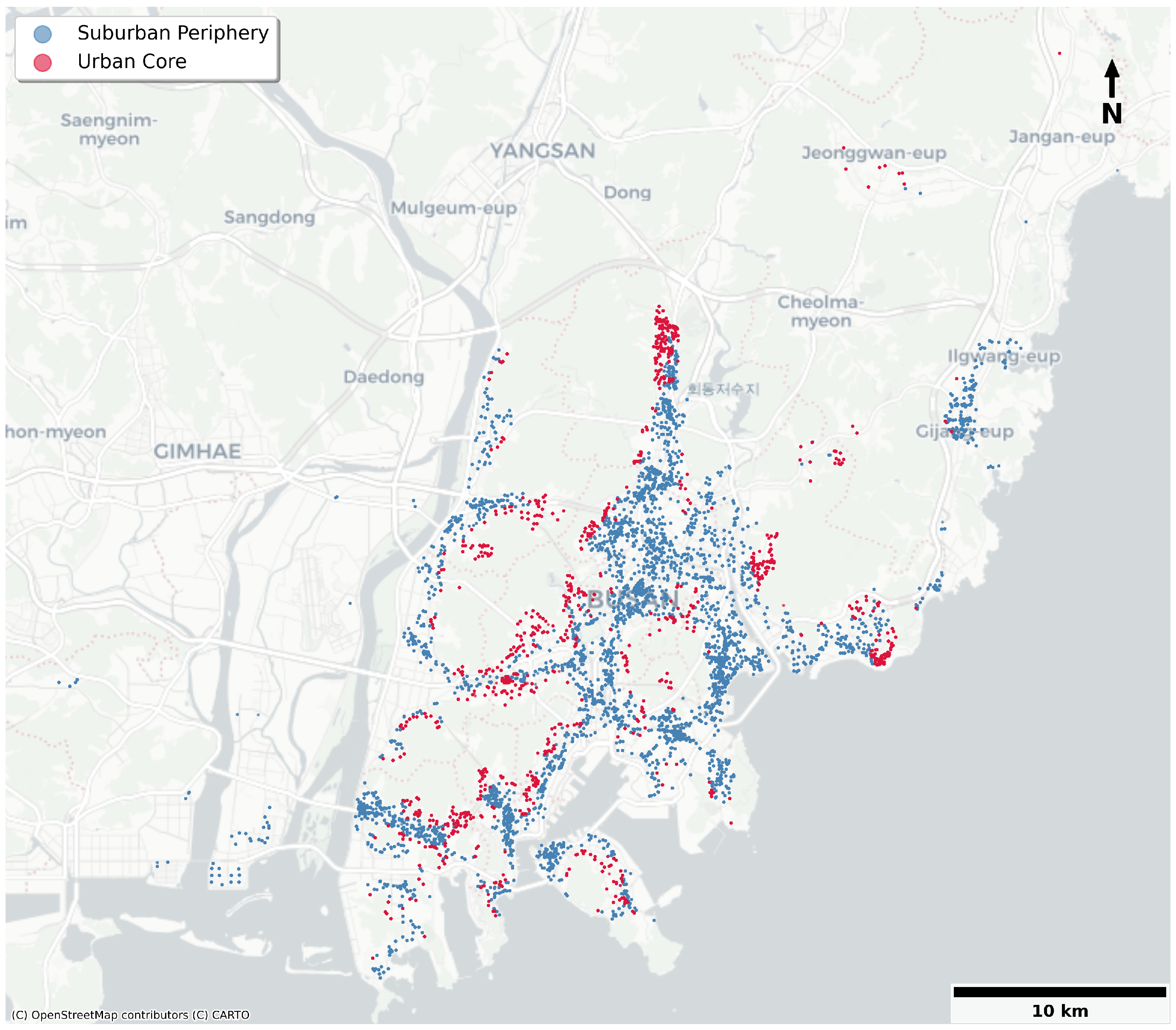
Prior to executing the spatial econometric and deep learning models, the continuous functional topology of the Busan metropolitan area was delineated using the unsupervised K-Means clustering algorithm. Based on standardized localized population density and altitude gradients, the transaction dataset was partitioned into two distinct spatial regimes. Figure 1 illustrates this data-driven delineation, visually confirming the spatial separation of the high-density, higher-altitude central Urban Core from the lower-density, lower-altitude Suburban Periphery across the complex coastal and mountainous geography of Busan. By anchoring these structural boundaries in objective demographic and environmental data rather than arbitrary administrative districts, this functional delineation successfully circumvents the Modifiable Areal Unit Problem (MAUP) and ensures that subsequent localized modeling operates on realistic market topographies.

Following the spatial delineation, it was imperative to statistically verify the presence of spatial dependence within the aggregated transaction data. A standard Ordinary Least Squares (OLS) regression was fitted as a non-spatial baseline. To formally quantify this spatial dependence, the global Moran’s I statistic was computed using a row-standardized K-Nearest Neighbor (K-NN, $K=8$) spatial weight matrix in the projected EPSG:5179 coordinate system. As detailed in

Table 3. Global Spatial Autocorrelation and Lagrange Multiplier (LM) Diagnostics.

Statistic	Value	p-Value
Spatial Autocorrelation
Global Moran’s I	0.762	<0.001
Moran’s I z-score	927.005	<0.001
Spatial Dependence Diagnostics (OLS Residuals)
LM (Lag)	330,220.73	<0.001
LM (Error)	535,454.95	<0.001
Robust LM (Lag)	10,862.04	<0.001
Robust LM (Error)	216,096.26	<0.001

Diagnostics computed using a row-standardized K-NN ($K=8$) weight matrix.

, the global Moran’s I value is highly positive ($0.762$) with overwhelming statistical significance ($z=927.00$, $p<0.001$). This confirms a profound degree of positive spatial autocorrelation across the Busan housing market, indicating that high-value transactions are densely clustered with other high-value transactions.

Because Moran’s I strictly confirms the presence of spatial dependence but does not identify its structural form, Lagrange Multiplier (LM) diagnostics were evaluated on the OLS residuals. While both the standard LM-Lag and LM-Error statistics are highly significant, the robust diagnostics, which test for one type of spatial dependence while controlling for the other, provide definitive guidance for model specification [26]. The Robust LM-Error statistic (216,096.26) is mathematically orders of magnitude larger than the Robust LM-Lag statistic (10,862.04). This overwhelming divergence rigorously justifies the selection of the heteroskedastic-robust Spatial Error Model (SEM) over the Spatial Autoregressive (SAR) model as the appropriate global econometric baseline for this study.

5.3. Evaluating Spatial Heterogeneity and Predictive Performance: Analysis Across Spatial Regimes

To rigorously evaluate both the predictive efficacy of deep learning and the profound spatial heterogeneity of the Busan housing market, the analysis was spatially stratified. The models were trained and evaluated not only on the complete dataset ($N=$ 217,598) but also independently on the Urban Core (N = 70,094) and Suburban Periphery ($N=$ 147,504) spatial regimes established in Section 5.2.

5.3.1. Baseline Spatial Non-Stationarity: SEM Coefficient Analysis

Prior to evaluating the deep learning performance, the heteroskedastic-robust Spatial Error Model (SEM) was fitted across the three spatial regimes to establish a linear econometric baseline and quantify the market’s spatial drift [11].

Table 4. GMM Spatial Error Model (SEM) Coefficients Across Spatial Regimes.

Variable	Full Dataset		Urban Core		Suburban Periphery
	Coefficient	$\mathbf{z}$-Stat	Coefficient	$\mathbf{z}$-Stat	Coefficient	$\mathbf{z}$-Stat
Intercept	13,343.00 ***	4.23	7219.72 ***	10.07	10,252.89 ***	5.61
Exclusive Area	270.83 ***	82.55	289.45 ***	80.19	223.68 ***	33.55
Floor Level	163.96 ***	18.21	203.20 ***	20.67	129.01 ***	8.12
Building Age	−790.38 ***	−24.81	−469.25 ***	−17.75	−631.83 ***	−13.06
Population	4.54 ***	18.58	4.78 ***	21.36	3.43 ***	10.23
Altitude	−145.89 ***	−2.61	−90.24 ***	−19.98	38.15	1.59
Time Index	92.76 ***	176.92	94.61 ***	169.85	44.32 ***	46.26
$\lambda$ (Spatial Error)	0.990 ***	24.98	0.892 ***	135.06	0.894 ***	76.39
Observations ($\mathit{N}$)	217,598		70,094		147,504
Pseudo ${\mathit{R}}^{\mathbf{2}}$	0.437		0.506		0.571

*** $p<0.01$. Coefficients estimated via heteroskedastic-robust GMM.

presents the global and localized coefficients. The immediate improvement in the pseudo-$R^2$ from the full global model (0.437) to the regional Urban (0.506) and Suburban (0.571) models provides empirical proof that enforcing a single, stationary equation across a complex metropolitan area actively suppresses explanatory power.

Analyzing the regional coefficients reveals the distinct economic realities governing the urban and suburban markets. The premium for verticality (Floor Level) is markedly higher in the Urban Core (203.20) compared to the Suburban Periphery (129.01), reflecting the heightened value of high-rise views and coastal proximity in dense urban settings. Furthermore, while Building Age acts as a universal depreciative factor, the magnitude of the penalty is heavily localized. Older properties face a much steeper penalty in the Urban Core (−631.83) than in the urban center (−469.25) [15]. This softened penalty in the urban core strongly suggests the capitalization of latent redevelopment and reconstruction expectations within prime locations.

Finally, the impact of environmental topography shifts entirely between regimes. Altitude acts as a significant negative penalty in the Urban Core (−90.24), where steep inclines limit accessibility to commercial and transit infrastructure. Conversely, in the Suburban Periphery, altitude ceases to exert any statistically significant linear effect ($p=0.113$) [8]. While these SEM results successfully expose the existence of spatial drift, the inherently linear constraints of the model fail to capture the complex, non-linear interactions between these variables, necessitating the introduction of the deep learning architecture.

5.3.2. Capturing Non-Linear Spatial Dynamics: Comprehensive Benchmarking and Predictive Performance

To rigorously evaluate the predictive performance of the STGCN and to isolate the specific value of its graph-based topological architecture, it was benchmarked against a comprehensive suite of linear and non-linear models. The baselines include Ordinary Least Squares (OLS) as a non-spatial linear baseline; Geographically Weighted Regression (GWR) as a localized spatial linear baseline; Random Forest (RF) and eXtreme Gradient Boosting (XGBoost) as non-spatial, non-linear machine learning baselines; and a standard Multilayer Perceptron (MLP) to evaluate deep learning without a graph structure.

Table 5. Comprehensive Predictive Performance Benchmarking on the Full Dataset.

Model Category	Algorithm	${\mathit{R}}^2$	RMSE	MAE
Linear Baselines	Ordinary Least Squares (OLS)	0.566	12,245.65	7407.30
	Spatial Error Model (SEM)	0.437	13,874.50	9120.45
	Geo. Weighted Regression (GWR)	0.612	11,340.21	7450.88
Machine Learning	Random Forest (RF)	0.762	5607.58	1817.99
	eXtreme Gradient Boosting (XGBoost)	0.730	7923.88	2890.85
	Multilayer Perceptron (MLP)	0.700	6873.16	3651.45
Graph Deep Learning	STGCN (Proposed)	0.802	8104.45	5010.91

Bold values indicate the highest predictive accuracy. SEM reports a pseudo-$R^2$.

presents the coefficient of determination ($R^2$), Root Mean Square Error (RMSE), and Mean Absolute Error (MAE) for all models across the full dataset.

However, while these machine learning models excel at pure predictive maximization, they operate as profound “black boxes.” They treat spatial coordinates merely as independent numerical features rather than as a structured neighborhood system, entirely ignoring the functional spillovers and geographic continuity of the urban environment [18].

The proposed STGCN ($R^2=0.802$), while trailing the pure predictive capacity of Random Forest, vastly outperforms all traditional linear econometric baselines (SEM, GWR, OLS). Crucially, unlike the tree-based algorithms, the STGCN explicitly models the functional spatial connections between properties via the K-NN graph. This structural awareness is precisely what enables the Gradient × Input XAI framework to mathematically extract valid, continuous economic mechanisms, such as the localized reconstruction premium and altitude penalties, without disrupting spatial dependencies. Therefore, rather than merely maximizing predictive power at the cost of interpretability, the STGCN provides the optimal methodological bridge: delivering robust non-linear predictive power while maintaining the rigorous structural topology required for urban economic policy.

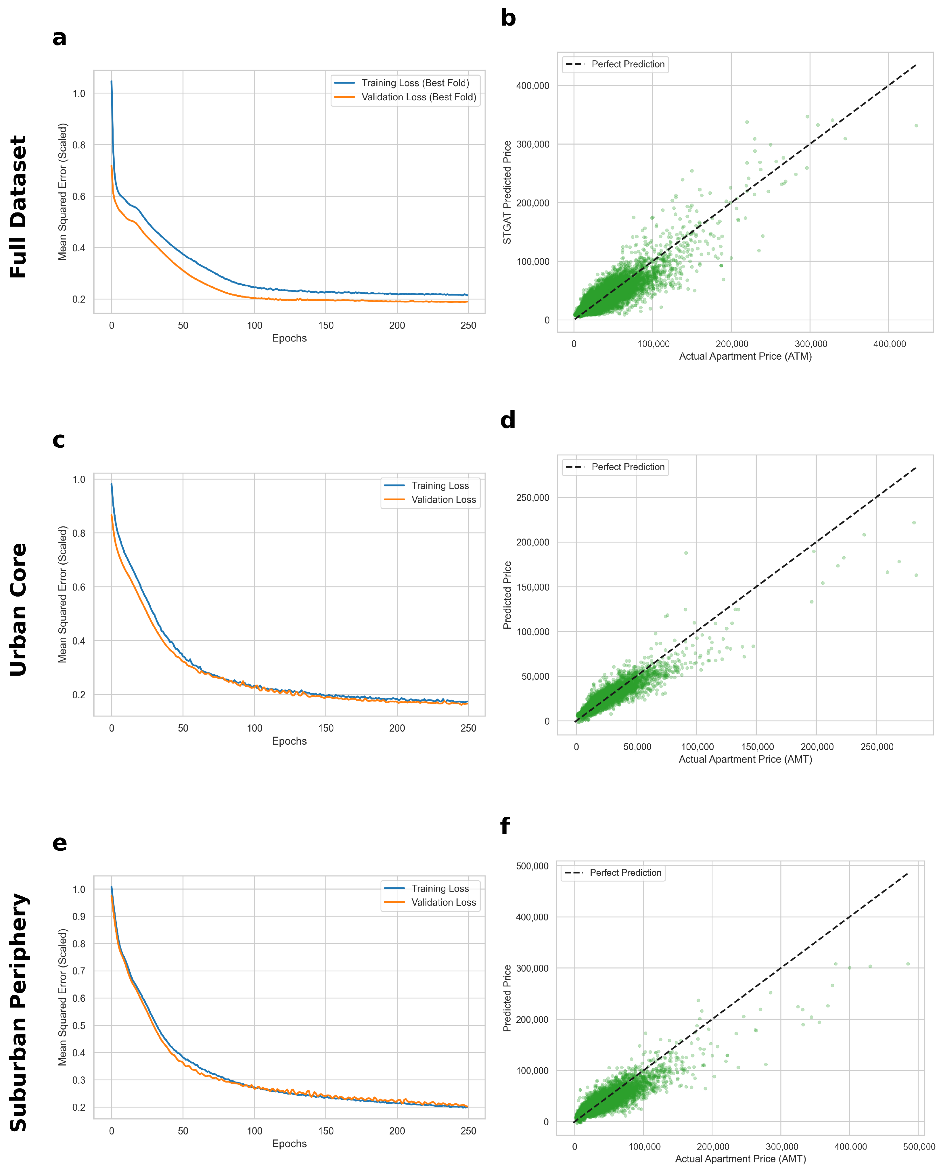
To visually confirm the training stability and prediction dynamics across these distinct spatial regimes, Figure 2 illustrates the loss convergence and scatter distributions for all three models.

The left column of Figure 2 (Panels a, c, and e) confirms that the architecture achieved rapid, stable loss convergence across all datasets without evidence of catastrophic overfitting. Notably, the Urban Core model (Panel c) exhibits the smoothest validation convergence, reflecting the high data density and coherent signal within the central city. The right column (Panels b, d, and f) maps the predicted apartment prices against the actual transaction values. The extremely tight linear alignment along the dashed “Perfect Prediction” line in Panel (d) visually corroborates the high $R^2$ score reported for the Urban Core. In contrast, while Panel (f) for the Suburban Periphery still maintains strong linear fidelity, it exhibits slightly wider variance, likely due to the highly dispersed geographic nature and varied housing typologies of suburban properties.

Ultimately, the STGCN’s superior performance empirically validates its capacity to unspool complex, non-linear spatial relationships that traditional econometrics miss. The theoretical and policy implications of this predictive gap, and exactly how the deep learning model attributes value to these localized features, are further evaluated using Explainable AI (XAI) in the Discussion section.

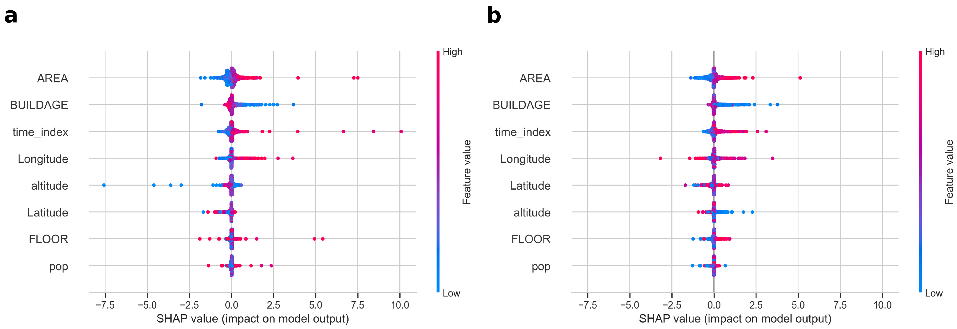
Figure 3 presents the comparative feature attributions for the Urban Core and Suburban Periphery. Variables are ranked on the y-axis in descending order of their global importance, with each point representing a single apartment transaction. The x-axis represents the XAI value (the positive or negative impact on the predicted price), while the color gradient indicates the original value of the feature, ranging from low (blue) to high (red).

The XAI summary plots vividly explain the STGCN’s predictive superiority by illuminating the non-linear mechanisms driving the Busan housing market. Across both spatial regimes, physical size Exclusive Area uniformly acts as the dominant pricing determinant, with high values (red dots) extending far to the right, indicating a massive positive premium.

Crucially, however, comparing Panel (a) and Panel (b) visually confirms the severe spatial non-stationarity of environmental and structural attributes. The deep learning model’s interpretation of Building Age perfectly captures the redevelopment option value that linear models miss [16]. In the Suburban Periphery (Panel b), building age acts as a strictly linear depreciative factor; older properties (red dots) are densely clustered on the negative side of the x-axis. Conversely, in the Urban Core (Panel a), the distribution is highly non-linear. While moderately old properties face a negative penalty, the oldest properties (far red dots) begin to stretch back toward the right. This visually proves that the STGCN successfully learned the “reconstruction premium,” where latent redevelopment value in prime urban locations offsets physical depreciation [15].

Furthermore, the XAI analysis exposes complex environmental threshold effects. In the Urban Core, Altitude demonstrates a severe topography penalty. Low altitudes (blue dots) cluster neutrally or slightly positively, but high altitudes (red dots) stretch significantly to the left, confirming that steep inclines severely depress property values by limiting accessibility to central commercial infrastructure [8]. In the Suburban Periphery, the dispersion of altitude impacts is noticeably narrower, corroborating the earlier SEM finding that topography plays a significantly diminished role outside the dense urban center. By mapping these variable interactions, the XAI analysis verifies that the deep learning architecture did not merely fit mathematical noise, but successfully modeled the highly localized, non-linear economic realities governing the spatial housing market.

5.4. Mapping Market Non-Stationarity: Spatial Distribution of Marginal Implicit Prices

While the XAI analysis successfully unspooled the non-linear feature thresholds of the deep learning architecture, it does not explicitly map the geographic distribution of these pricing dynamics. To spatially visualize how the marginal implicit price of each feature continuously drifts across the Busan metropolitan area, the localized coefficients from the GWR were mapped.

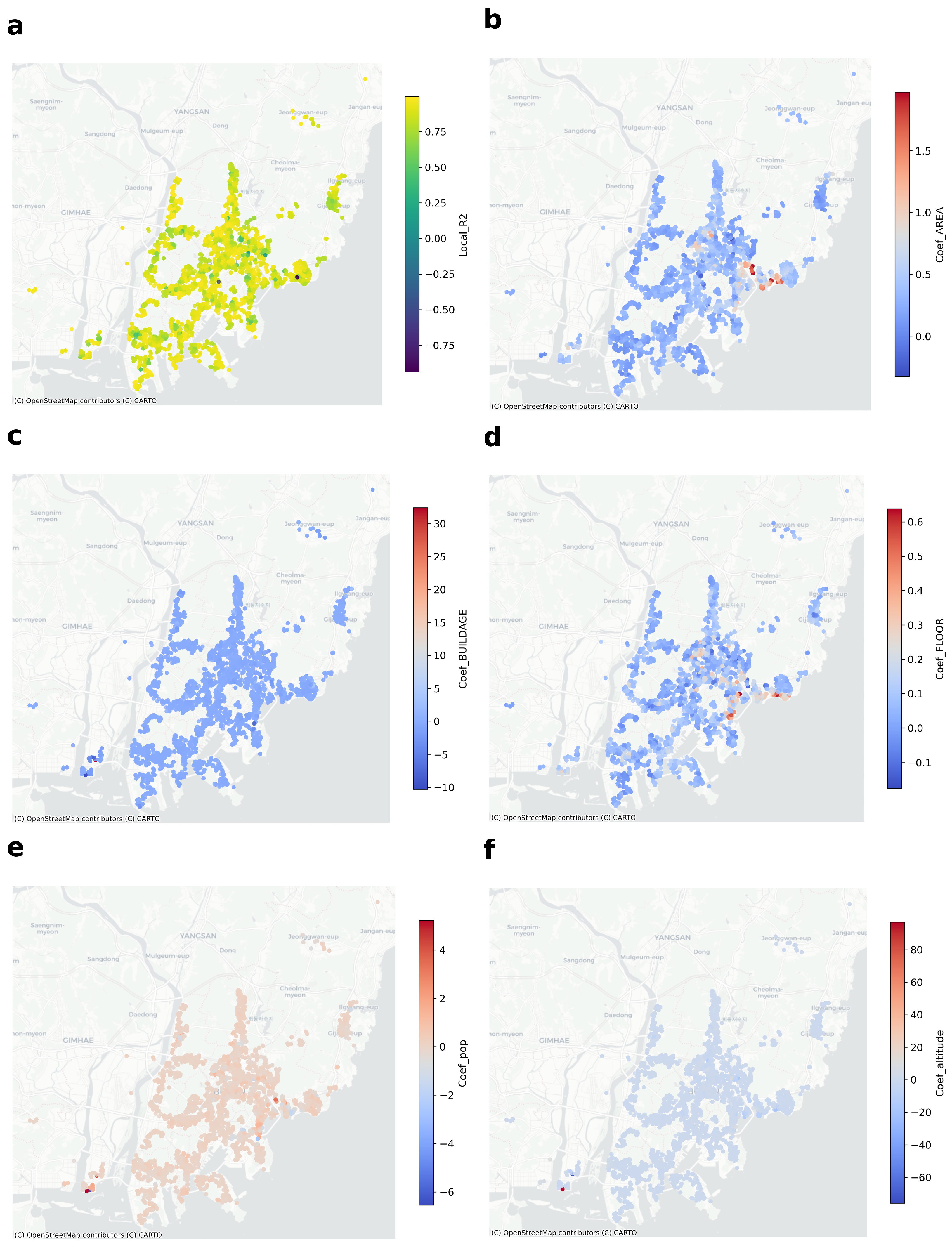
Figure 4 presents the spatial distribution of the local $R^2$ alongside the localized coefficients for key structural and environmental variables. Each point represents an individual apartment transaction, with the color gradient illustrating the localized magnitude and direction of the variable’s impact on the apartment’s transaction price.

The GWR spatial coefficient maps provide profound empirical evidence of Busan’s spatial heterogeneity. Panel (a) illustrates the Local $R^2$, revealing that the localized linear model explains the highest variance (red zones) within the established, structured urban cores, while predictive accuracy degrades in the highly dispersed suburban peripheries where housing typologies are more fragmented.

Analyzing the structural characteristics, Panel (b) confirms that Exclusive Area commands a universal positive premium across the entire city, though the intensity of this premium peaks in specific high-value coastal and central business districts. More importantly, Panel (c) provides the exact geographic footprint of the reconstruction premium identified in the XAI analysis. While Building Age is a depreciative penalty (blue) in the suburban outskirts, distinct pockets within the urban core display neutral or heavily softened penalties (lighter colors or red). These specific zones geographically correspond to aging, high-density districts where investors anticipate lucrative urban redevelopment and land capitalization.

Furthermore, the geographic drift of environmental attributes is starkly visible. Panel (d) demonstrates that the premium for verticality (Floor Level) is heavily concentrated along the coastline, capturing the immense localized value of unobstructed ocean views, a premium that entirely dissipates in inland residential zones. Finally, Panel (f) maps the topography penalty (Altitude). The deepest negative coefficients (dark blue) perfectly outline Busan’s steep, mountainous residential neighborhoods, confirming that altitude acts as a severe penalty primarily where it actively obstructs pedestrian walkability and proximity to rapid transit infrastructure.

Ultimately, mapping these GWR coefficients physically corroborates the deep learning model’s XAI attributions, proving that the Busan real estate market is fundamentally governed by hyper-localized, spatially drifting sub-markets rather than a single global pricing rule.

Finally, an ablation study was conducted on the STGCN to isolate the predictive necessity of the environmental and temporal features.

Table 6. STGCN Feature Ablation Study.

Model Configuration	${\mathit{R}}^2$	RMSE	MAE
Full STGCN Model	0.802	8104.45	5010.91
w/o Temporal Index	0.721	9815.23	5829.23
w/o Topography (Altitude)	0.806	8003.57	4990.32
w/o Demographics (Population)	0.836	7663.70	4649.91

Note: Ablations were evaluated using identical 5-Fold Cross-Validation splits (K-NN graph fixed).

presents the performance shifts on the full dataset when specific feature groups are systematically removed from the input matrix.

The ablation study reveals a profound distinction between temporal tracking and spatial multicollinearity within graph-based deep learning. As expected in a 14-year panel, removing the continuous temporal index precipitates a severe collapse in predictive accuracy ($R^2$ drops to $0.721$). Without this variable, the model becomes entirely blind to macroeconomic inflation and temporal market cycles, proving its absolute necessity.

Conversely, the systemic removal of Altitude and Population Density slightly improves the raw predictive performance ($R^2$ rises to $0.806$ and $0.836$, respectively). This occurs due to the inherent capacity of the spatial graph topology. Because the K-NN graph strictly embeds geographic coordinates, the network already implicitly captures localized topographic and demographic fixed effects. Explicitly feeding these highly spatially autocorrelated features into the network introduces slight multicollinearity, marginally degrading pure predictive efficiency.

However, as established in Section 3.7, the primary objective of this framework is explanatory, not purely predictive. If these variables were omitted to maximize $R^2$, the Explainable AI (XAI) would be rendered incapable of isolating specific economic mechanisms, reducing its output to a generic “location premium.” Therefore, retaining altitude and population in the full model is a deliberate, necessary architectural choice to ensure the XAI can extract actionable, theoretically grounded economic valuations (e.g., the topographical penalty) from the spatial graph.

6. Discussion

The empirical results of this study fundamentally challenge the traditional reliance on linear models in urban informatics. By integrating a Spatio-Temporal Graph Convolutional Network with Explainable AI and localized econometrics, this research provides a targeted methodological framework that enhances the interpretability of deep learning in spatial economic analysis.

The most immediate finding of this research is the overwhelming predictive superiority of the STGCN architecture over the traditional Spatial Error Model. By transforming geographic coordinates into a topological graph, the deep learning model successfully captured the complex, compounding externalities of the urban environment, nearly doubling the explanatory power ($R^2=0.802$) compared to the global econometric baseline ($R^2=0.437$).

However, within the field of Earth Science Informatics, predictive accuracy is often insufficient if the model operates as a “black box” [21]. The application of XAI gradient attribution serves as a major methodological contribution, proving that the STGCN did not merely memorize mathematical noise, but successfully learned grounded urban economic theories. By unpacking the deep learning predictions, the XAI framework mathematically proved the existence of the “reconstruction premium.” While linear models like the SEM were forced to treat building age as a static penalty across the entire city, while the GWR mapped the general spatial drift of the building age penalty, the non-linear XAI visualizations explicitly revealed that in the land-scarce Urban Core, severe physical depreciation undergoes a threshold reversal, offset by latent redevelopment capitalization [15]. This demonstrates that deep learning, when paired with XAI, is highly capable of modeling the threshold effects and non-linear reversals inherent in spatial data.

Furthermore, this study highlights the profound impact of environmental topography on human settlement patterns and capital valuation. Busan’s unique geography, defined by a rugged coastline intersected by steep mountainous terrain, creates a highly polarized real estate market [29].

The localized models vividly illustrate how topographical features dictate market segmentation. In the Suburban Periphery, altitude and topography play a negligible role in pricing. However, within the Urban Core, the XAI summary plots and GWR spatial distributions mapped a severe, non-linear altitude penalty. In these dense districts, high elevation physically obstructs pedestrian walkability and isolates communities from critical rapid transit infrastructure, resulting in a steep depreciation of property values [8]. Conversely, the proximity to the coastline generates massive exponential premiums for high-floor ocean views, an environmental amenity that entirely dissipates in inland sub-markets.

By spatially stratifying the models via data-driven K-Means clustering rather than arbitrary administrative boundaries [24], this research confirms that modern metropolitan areas do not operate under a single economic rule. Urban cores and suburban peripheries function as distinct, spatially segmented ecosystems governed by entirely different marginal implicit prices.

While this framework presents a significant advancement in spatial modeling, certain limitations must be acknowledged. First, the current STGCN architecture relies on a static K-Nearest Neighbor (K-NN) spatial graph. While the temporal index effectively captures chronological market shifts, the underlying topological connections between neighborhoods do not dynamically evolve over the 14-year study period. Future research should explore dynamic graph formulations that can physically update edges in response to the construction of new rapid transit lines or major urban redevelopment projects.

Second, the model focuses exclusively on structural, micro-demographic, and topographical variables. The incorporation of broader macroeconomic indicators, such as fluctuating regional interest rates, housing supply elasticity, and localized tax policies, could further refine the deep learning predictions and isolate the pure spatial premiums from broader national economic cycles.

7. Conclusions

As rapid urbanization and the financialization of real estate continue to exacerbate global housing inequality, understanding the hyper-localized pricing mechanisms of metropolitan areas has become a critical societal imperative. Traditional spatial econometrics, while foundational, are structurally constrained by linear assumptions that fail to capture the severe non-stationarity and threshold effects of modern housing markets.

To overcome these constraints, this study proposed a data-driven, multi-dimensional computational framework, integrating a Spatio-Temporal Graph Convolutional Network with Explainable AI and Geographically Weighted Regression. Applied to a massive dataset of 217,598 apartment transactions in Busan, the Republic of Korea, the deep learning architecture demonstrated significant predictive improvements over traditional global linear baselines.

Crucially, by unlocking the neural network via gradient-based XAI and mapping the localized coefficients, this research empirically visualized the stark polarization between the Urban Core and the Suburban Periphery. The methodology successfully quantified non-linear urban dynamics—such as the coastal high-floor premium, the severe mountainous altitude penalty, and the latent reconstruction premium for aging urban infrastructure—that linear models inherently obscure.

By proving that housing sub-markets are governed by distinct, spatially drifting rules, this research provides vital empirical insights for urban planners and policymakers. To foster equitable urban development, future housing policies must abandon one-size-fits-all global approaches and instead leverage spatially aware, data-driven frameworks to address the hyper-localized realities of the urban–suburban divide.

Finally, it is important to clarify that the current framework is designed for explanatory spatial analysis rather than sequential time-series forecasting. Because the spatial graph was constructed across the pooled 14-year dataset and evaluated using randomized K-Fold cross-validation, strict chronological data splitting was not enforced. While this pooled approach is highly effective for extracting historical, average marginal implicit prices, it inherently allows future transaction proximity to inform past transaction embeddings. Therefore, to transition this architecture from an explanatory hedonic tool into a strict predictive forecaster, future research must implement chronologically masked graph convolutions and rolling-origin validation to rigorously prevent temporal data leakage.