1. Introduction
In recent years, global tourism has grown rapidly, but “overtourism” has intensified, placing heavy pressure on ecosystems, infrastructure, and residents’ quality of life [
1,
2,
3,
4,
5]. Sustainable tourism seeks economic benefits with minimal environmental and social costs [
6,
7,
8], yet balancing growth with ecological protection remains a persistent challenge—particularly in destinations where tourism dominates the local economy.
Existing studies on policy evaluation, tourist flow regulation, and carbon accounting often fail to capture multi-objective trade-offs involving revenue, emissions, and infrastructure [
9,
10]. A critical limitation in these approaches is the prevalent reliance on linear assumptions, which assume constant proportional relationships between tourist numbers and their impacts. However, recent empirical research increasingly demonstrates that the relationship between tourism growth and environmental or social outcomes is inherently non-linear. For instance, studies on the Tourism Environmental Kuznets Curve (TEKC) have identified distinct threshold effects, where carbon emissions accelerate exponentially once tourist arrivals exceed a specific carrying capacity [
11,
12]. Similarly, overtourism scholars observe that congestion costs and resident dissatisfaction follow a non-linear trajectory: Maggi and Bertocchi (2025) argue that when visitor density surpasses critical tipping points, it triggers a disproportionate decline in destination efficiency and visitor satisfaction due to saturation [
13,
14]. Ignoring these non-linear dynamics risks generating planning strategies that underestimate the compounding risks of high-intensity tourism.
Juneau, Alaska, exemplifies these tensions. As the state capital and a premier cruise destination, Juneau receives over 1.7 million visitors annually—predominantly during the summer cruise season—despite a permanent population of fewer than 32,000 [
3]. This extreme visitor-to-resident ratio strains roads, waste systems, and fragile alpine and marine ecosystems, while simultaneously underpinning the local economy. The city thus represents an ideal testbed for modeling the nonlinear trade-offs between economic dependency and ecological resilience in overtourism contexts.
To address these challenges, this study makes three specific contributions:
- (1)
We develop a multi-objective nonlinear optimization model that explicitly incorporates threshold-based functional forms to capture the complex, non-proportional relationships among tourist volume, tax revenue, carbon emissions, and infrastructure costs—thereby overcoming the limitations of linear frameworks;
- (2)
We integrate real-world policy constraints (e.g., emission ceilings, fiscal feasibility) and solve the model using a genetic algorithm to derive actionable, Pareto-efficient policy levers, such as optimal visitor caps and tourism tax rates;
- (3)
We validate the model’s generalizability through cross-case applications in Venice—a global icon of overtourism—and Kodiak—an underutilized Alaskan destination— demonstrating its adaptability for both containment and sustainable growth strategies.
Therefore, we hypothesize that sustainable tourism planning must explicitly account for nonlinear threshold effects in the relationships among tourist volume, economic returns, carbon emissions, and infrastructure costs to achieve Pareto-optimal and ecologically viable outcomes. Building on this hypothesis, our multi-objective nonlinear optimization framework offers a decision-support tool for destinations worldwide seeking to navigate the delicate balance between tourism-driven prosperity and long-term sustainability.
2. Related Work
2.1. Research on Sustainable Tourism Development
Sustainable tourism aims to satisfy current tourist demand while ensuring resources for future generations [
6,
7,
8]. Early studies examined environmental impacts and carrying capacity [
15,
16,
17]; e.g., Buckley [
18] used ecological footprint analysis, while Hunter [
15] developed a framework combining economic, social, and ecological indicators. With climate change gaining attention, research increasingly analyzed tourism-related emissions and mitigation [
10,
19], such as Gössling et al. [
1] on emission structures and low-carbon strategies.
Recently, multi-objective optimization has been applied to balance economic, environmental, and social benefits [
20,
21,
22]. Examples include linear programming for capacity control [
2], system dynamics for policy simulations [
23], and MCDA-based collaborative frameworks [
9]. Yet, these models struggle with nonlinear interdependencies among taxation, infrastructure costs, and emissions, limiting refined optimization.
2.2. Applications of Multi-Objective Optimization and Genetic Algorithms in Tourism Management
Multi-objective optimization enables Pareto-efficient trade-offs across objectives [
24]. Deb et al. [
25] summarized its theoretical foundations. Among metaheuristics, genetic algorithms (GA) are widely applied in tourism for their global search ability and low modeling requirements [
26,
27]. Luo et al. [
28] used GA to optimize tourist flow and reduce congestion, while Kumar and Singh [
29] integrated GA with fuzzy programming for pricing and capacity allocation.
GA also handles nonlinear and non-convex problems in forecasting and policy simulation [
30]. Coello et al. [
31] showed adaptive crossover and mutation improve diversity and convergence. These approaches provide the methodological basis for our framework.
2.3. Carbon Emission Accounting and Mitigation Strategies
Carbon accounting is vital to assessing tourism’s environmental impact [
10]. Scott et al. [
19] found tourism contributes about 8% of global emissions, mainly from transport. Becken and Patterson [
32] proposed an LCA-based framework. Mitigation strategies involve supply-side measures (green energy, infrastructure) and demand-side measures (behavioral guidance) [
33]. Carbon taxation and emissions trading have also been explored [
34,
35], closely linked to tax optimization.
2.4. Infrastructure Carrying Capacity
Infrastructure capacity constrains sustainable tourism [
36]. Bramwell and Lane [
37] introduced environmental thresholds in investment planning, while Nguyen et al. [
38] optimized facility layout via multi-objective planning. Tax feedback mechanisms reinvesting revenues into infrastructure and protection [
39,
40] have been shown to extend destination lifecycles and improve satisfaction.
2.5. Summary
Research has advanced sustainable tourism modeling, emission accounting, and infrastructure planning, but integrated frameworks covering economic, tax, emission, and cost factors remain scarce. This paper addresses this gap by developing a multi-objective nonlinear optimization model with GA and sensitivity analysis to jointly optimize tourist flows and tax policies, supporting balanced economic, environmental, and social outcomes.
The contributions are as follows:
A comprehensive model integrating revenue, taxation, emissions, and infrastructure costs.
A solution framework combining sub-models, sensitivity analysis, and GA for robust global optimization.
Validation across destinations of different scales (Juneau, Venice, Kodiak), demonstrating adaptability and transferability.
3. Our Work
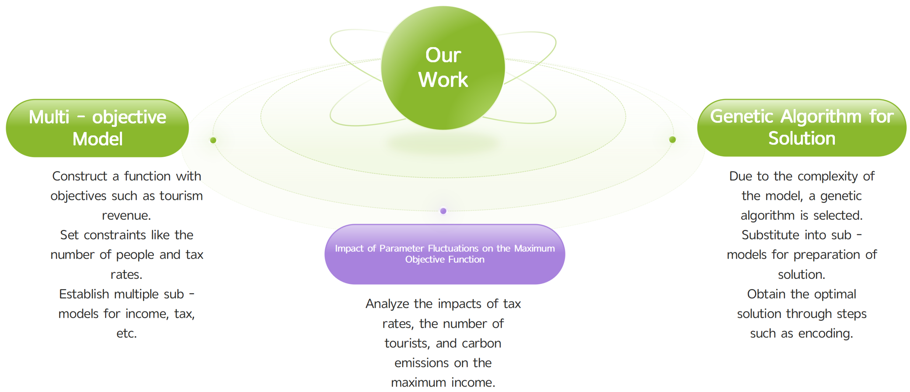
As shown in
Figure 1, this paper constructs a multi-objective optimization model centered on income, taxation, carbon emissions, and infrastructure costs. Combined with parameter sensitivity analysis and solved using genetic algorithms, this model provides quantitative decision support for sustainable tourism development. The key mathematical notations used in this paper are listed in
Table 1.
Table 2 presents descriptive statistics for the four core variables used in our optimization model, covering annual data from 2019 to 2023. The sharp decline in tourist volume in 2020–2021 reflects pandemic-related disruptions, followed by a strong rebound in 2022–2023. Correspondingly, tax revenue and carbon emissions exhibit high volatility (coefficient of variation > 40%), underscoring the need for robust policy design under uncertainty. Infrastructure costs remain relatively stable, indicating fixed operational baselines despite visitor fluctuations.
Assumptions and Justifications
To ensure the feasibility and tractability of the proposed model, several assumptions are introduced and justified as follows:
Assumption 1: No special environmental factors or abnormal tourist demands will occur during the model operation. Justification: Such factors are highly unstable and may lead to inaccuracies in the model solution.
Assumption 2: The policies implemented and the situations faced by Juneau City in 2026 are assumed to be consistent with those in 2023. Justification: If the implemented policies change significantly, the results derived from the model would no longer be applicable to reality.
4. Construction of Sustainable Tourism Industry Model
4.1. Data Description
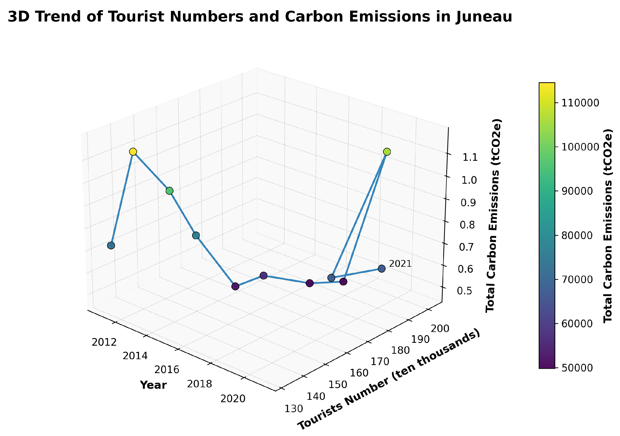
We collected multi-year data on tourist numbers, revenues, taxes, infrastructure costs, and carbon emissions in Juneau. As shown in
Figure 2, all indicators exhibited steady growth: increasing tourist arrivals and revenues were accompanied by rising emissions and infrastructure costs, indicating strong correlations among the variables. It should be noted that these data differ from conventional datasets commonly used in computer science research, as they are derived from real-world long-term statistics and monitoring records, thereby ensuring high authenticity and reference value.
A strong positive, nonlinear relationship exists between visitor numbers and carbon emissions: as tourist flows rise, energy use and transport increase disproportionately, intensifying emissions. This underscores the environmental burden of tourism expansion and the need to embed emission constraints in sustainable planning.
4.2. Objective Functions
To address the tourism problem and promote sustainable development in Juneau, we establish a multi-objective optimization model with four goals: tourism revenue, tax revenue, carbon emissions, and infrastructure costs. In order to integrate these objectives into a unified framework, we construct a comprehensive objective function
Z by applying weighted coefficients. The objective function to be maximized is expressed as
Here, Z represents a dimensionless index of overall sustainability performance, constructed by balancing economic gains against environmental and infrastructural costs; it is not a utility function but a policy-oriented composite indicator.
Where
denote the weights assigned to tourism revenue, tax revenue, carbon emissions, and infrastructure costs, respectively. These weights satisfy the normalization condition
Here, N denotes the actual number of tourists; represents the total tourism revenue; indicates the tax revenue generated by tourism; corresponds to the carbon emissions; and reflects the infrastructure costs.
When evaluating different weight configurations, the relative importance of these objectives may vary, leading to different optimization sensitivities. To simplify the analysis, we adopt a general case in which all weights are assumed to be equal, allowing us to focus on identifying the optimal solution of the comprehensive objective function without explicitly considering weight variation.
4.2.1. Constraint Conditions
In order to ensure the rationality and sustainability of the optimization model, the following constraints are imposed:
Tourist number constraint:
where
N is the actual number of tourists and
is the maximum allowable capacity of scenic spots. This constraint ensures that the number of visitors does not exceed the upper limit, thereby preventing irreversible damage caused by overcrowding.
Tax rate constraint:
where
denotes the tax rate. The tax rate must remain within a reasonable range: if set too low, fiscal revenue will be insufficient; if set too high, it will discourage tourism and hinder market development. This paper examines several major economies, including the maximum tax rates applicable in each country. The maximum tax rate is set at 45% for the purposes of this study.
Carbon emission constraint:
where
represents carbon emissions generated by tourism, and
is the maximum acceptable threshold. This condition guarantees that emissions remain within environmentally sustainable limits.
Infrastructure cost constraint:
where
is the infrastructure cost and
is the total tourism revenue. This constraint ensures that the investment in infrastructure does not exceed the revenue generated by tourism, maintaining the economic viability of development.
4.2.2. Sub-Models
- (1)
Revenue calculation model.
The total revenue generated from tourism is assumed to be positively correlated with the number of visitors. If the average expenditure per visitor is denoted as a constant
M, then the total revenue can be formulated as:
where
N represents the actual number of visitors, and
M denotes the average spending per visitor.
However, visitor consumption patterns are often influenced by various external factors such as seasonal fluctuations, regional characteristics, and overall market conditions. To account for these influences and improve model accuracy, a correction factor
is incorporated into the revenue function. Thus, the adjusted model becomes:
where
is a function of the visitor volume, reflecting that total revenue may vary nonlinearly with changes in the number of tourists.
- (2)
Tax calculation model.
Taxes are assumed to be linearly proportional to the total tourism revenue. Thus, the tax revenue function can be defined as:
where
denotes the tax rate, and
represents the total tourism revenue.
- (3)
Carbon emission model.
Carbon emissions
are considered to have a nonlinear relationship with the number of visitors
N. The basic form of the model is expressed as:
where
n is an exponent that captures the nonlinear influence of visitor numbers on carbon emissions, and
k is a constant representing the average carbon emissions per visitor.
To further improve model accuracy, external factors such as seasonal variations and technological progress are considered. By introducing a correction function
, the refined model becomes:
where
adjusts the emission estimation under varying conditions.
- (4)
Infrastructure cost model.
Infrastructure cost
is assumed to have a nonlinear relationship with the number of visitors
N. In addition, part of the tax revenue is reinvested into infrastructure improvements. The model is initially defined as:
where
is the infrastructure cost coefficient (usually a constant),
denotes the proportion of tax revenue allocated to infrastructure, and
is the total tax revenue.
To enhance accuracy, we further consider additional factors such as infrastructure aging and maintenance. By introducing a correction factor
, the model is refined as:
where
represents the aging or maintenance effect of infrastructure.
- (5)
Actual visitor number model.
Changes in the tax rate may lead to nonlinear fluctuations in visitor numbers. Since visitors exhibit varying sensitivities to tax burdens, and external factors such as seasonal variations or economic cycles may also play a role, the actual number of visitors
N is modeled as:
where
denotes the tax rate,
is the maximum potential number of visitors, and
is a sensitivity function that reflects how visitor numbers respond to changes in taxation.
4.3. Relationship Between Objectives
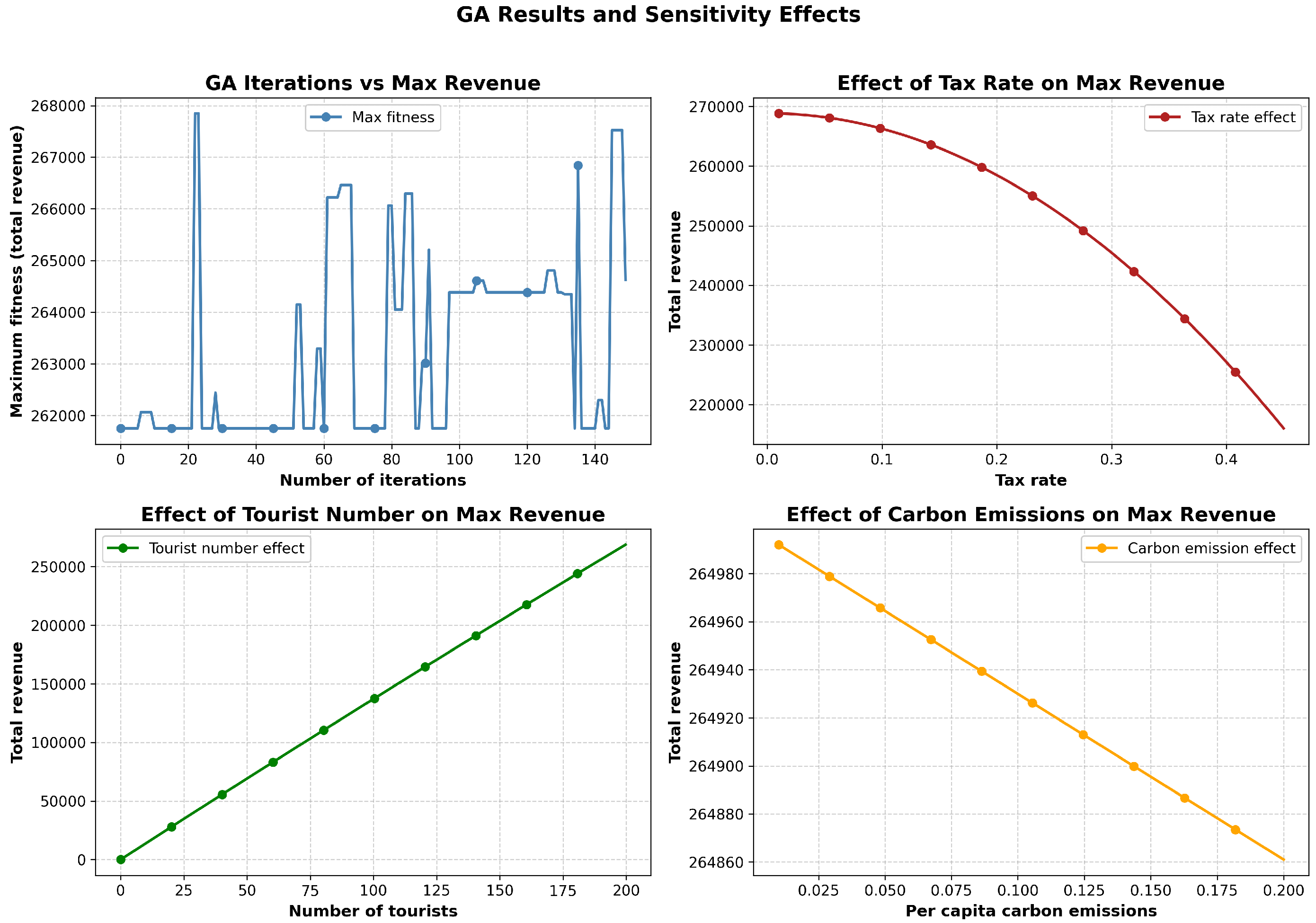
Figure 3 shows that moderate tax increases promote revenue growth, but excessive rates (near 0.45) suppress it. Likewise, rising tourist numbers initially boost revenue, yet excessive growth (around 199.75) causes diminishing returns. Moreover, higher carbon emissions reduce revenue by reflecting greater environmental stress and management costs.
4.4. Expenditure of Additional Revenue
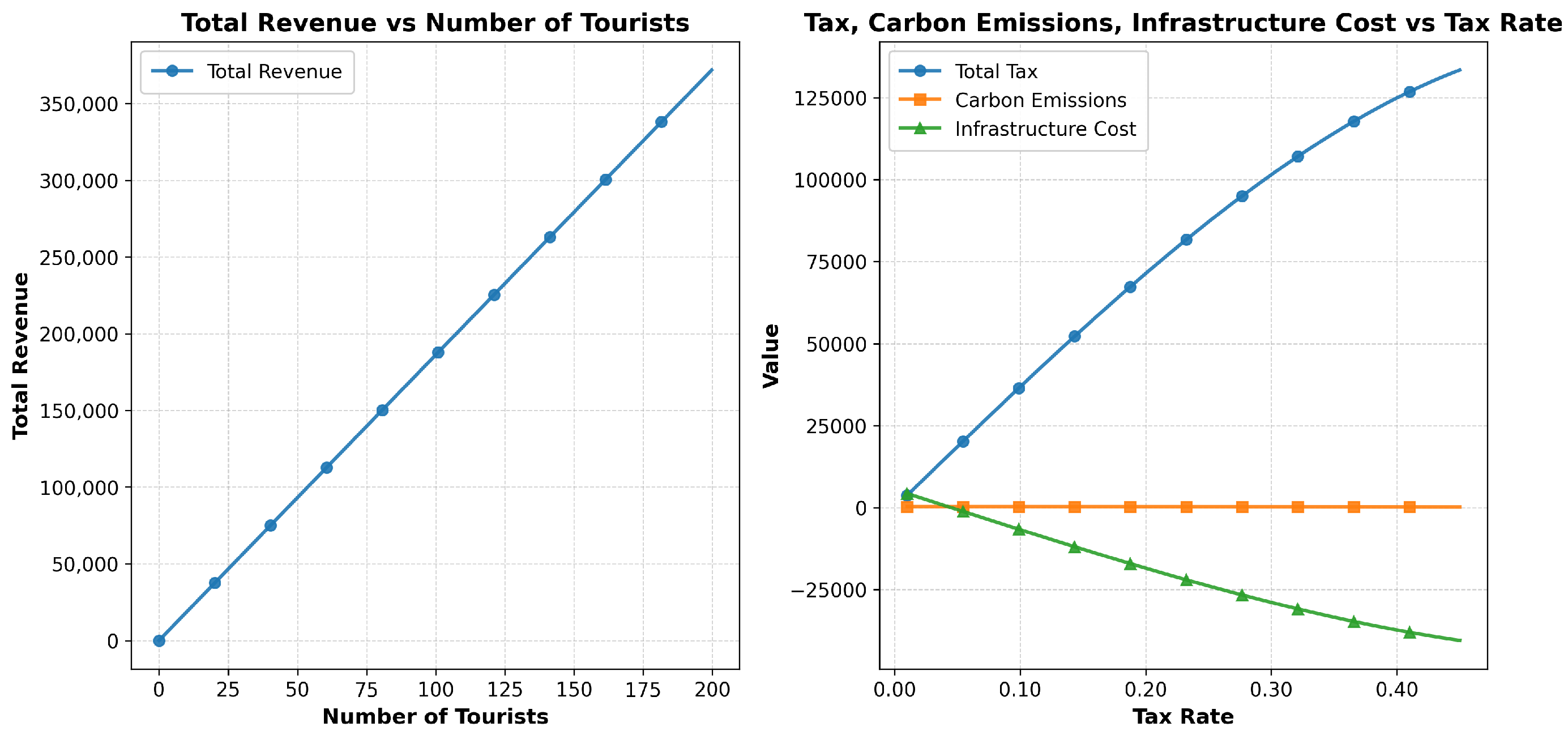
The additional revenue generated through taxation serves as a critical factor in influencing the comprehensive objective function. It is essential to analyze how taxation impacts this function and how the resulting feedback can be incorporated into the previously established model. Accordingly, we solved the related sub-model, and the obtained results are presented in the following
Figure 4.
From the figure above, the following conclusions can be summarized:
Owing to the linear relationship between tax revenue and the tax rate, an increase in the tax rate results in a continuous rise in total tax revenue.
The infrastructure cost is defined as
By combining this formula with the figure, it can be observed that infrastructure cost decreases as the tax rate increases.
The simultaneous growth in tax revenue and reduction in infrastructure cost enhance the comprehensive objective function. In this process, the additional revenue is integrated back into the established model through the variation in infrastructure cost.
5. Model Solving
5.1. Data Processing
To construct a sustainable tourism model for Juno City and ensure its applicability in the coming years, we incorporate projections for 2026 as the reference data, thereby enhancing the rationality and feasibility of the proposed framework.
5.1.1. Prediction of the Maximum Number of Tourists in 2026
Data Preparation
According to the Alaska Visitor Volume Report 2023 (Version 24 7.12.24 rev FINAL), Juneau City has become a popular tourist destination. The number of cruise tourists has steadily increased, rising from approximately million in 2019 to million in 2023.
Modeling and Analysis
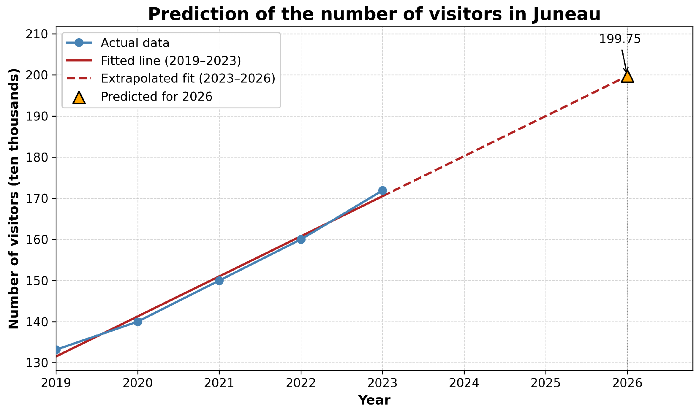
To estimate the potential maximum number of tourists in 2026, a mathematical model was constructed based on historical data. The years 2019 and 2023 were encoded as 0 and 4, respectively, with the corresponding number of tourists as the target variable. A linear regression model was then built using the LinearRegression class in the scikit-learn library and trained by minimizing the sum of squared errors between predicted and observed values.
With the regression model, the year 2026 was encoded as 7, and the expected tourist number was predicted using the model’s
predict function. Visualization was conducted with the
matplotlib library to display actual data points, the fitted regression line, and the extrapolated prediction, as shown in
Figure 5. The final estimated tourist capacity for Juneau in 2026 is denoted as
(measured in units of
people).
5.1.2. Solve for , , k and M
As shown in
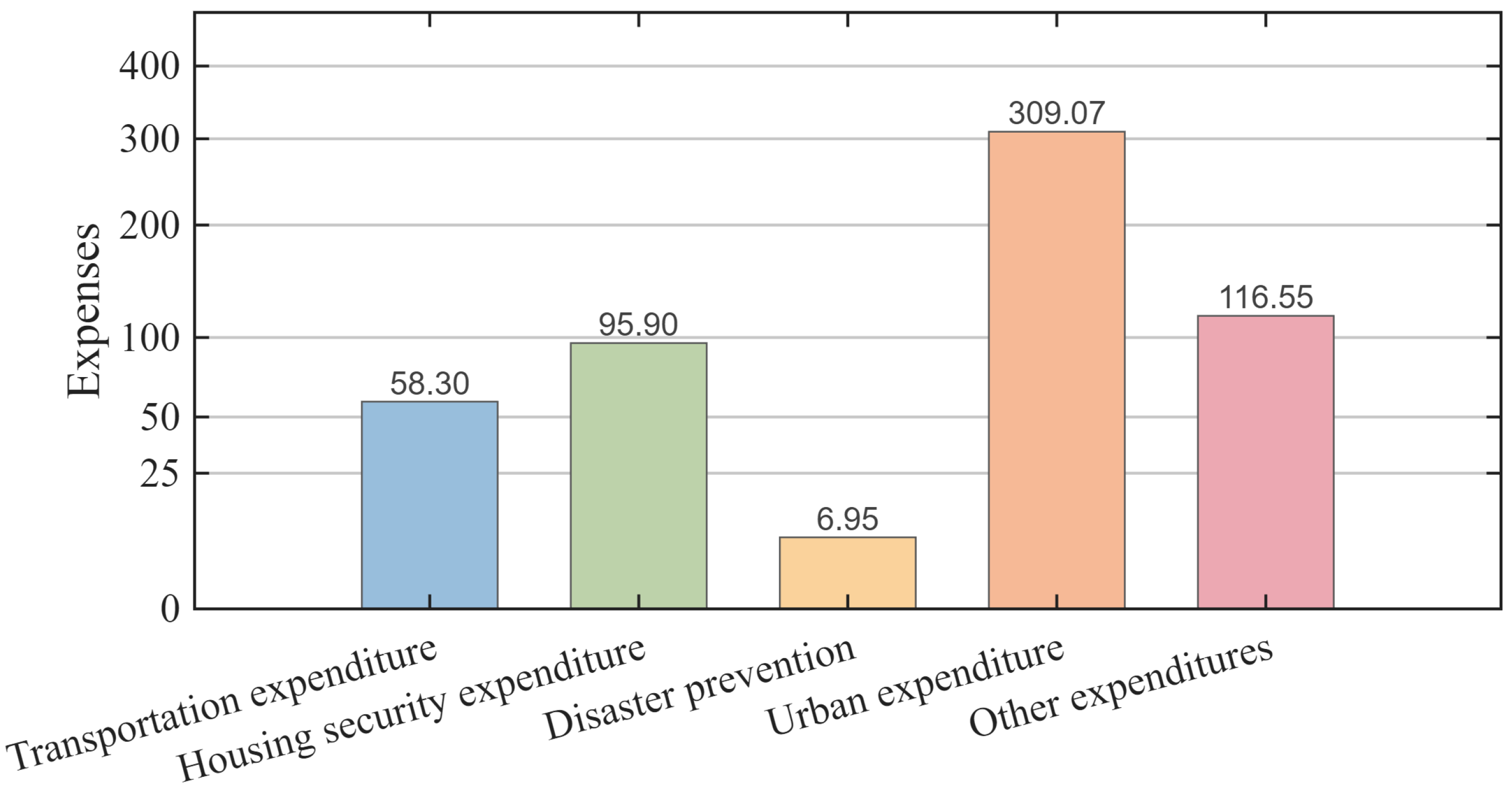
Figure 6, the government’s fiscal expenditure is distributed across five major categories.
(1) According to the official statistics, the government’s fiscal expenditure is summarized in
Figure 6. The coefficient
is calculated as
which yields
(2) The additional revenue from taxation is allocated to environmental protection, infrastructure construction, and community development projects. Therefore, the allocation coefficient is defined as
(3) Based on the data, the total carbon dioxide emissions from electricity consumption in Juneau amounted to
kilograms, with the per capita emissions being
kilograms. Hence, the coefficient
k is given by
(4) According to the “CBJ-Cruise-Impacts-2023-Report-1.22.24” [
3], the total expenditure of cruise passengers in Juneau in 2023 was approximately 320 million. Furthermore, the “Alaska Visitor Volume Report 2023–2412.24 rev FINAL” [
4] indicates that Juneau received about
million cruise tourists in 2023. Thus, the per capita expenditure
M is calculated as
5.1.3. Solve for Carbon Emission Maximum
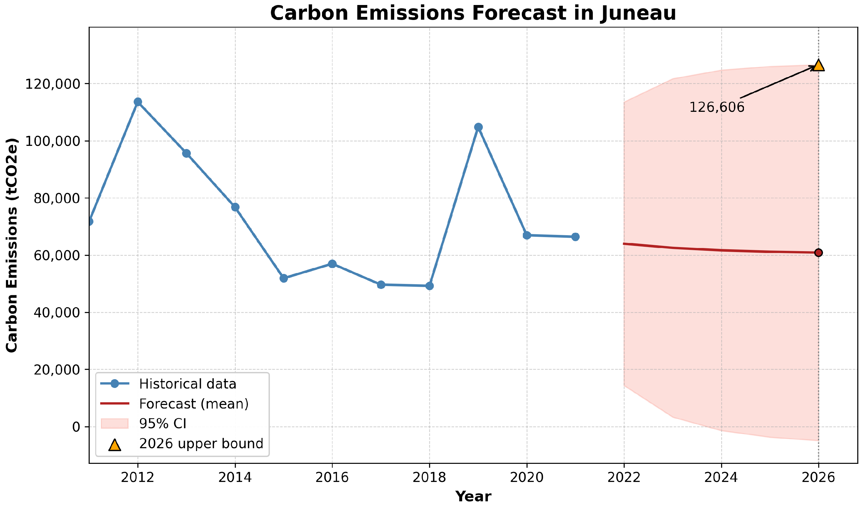
We used Juneau’s annual CO2, CH4, and N2O emission data (2011–2021), aggregated by year to construct a time series dataset. Total carbon emissions were obtained by summation, forming the basis for prediction.
The Auto-Regressive Integrated Moving Average (ARIMA) model was applied, as it effectively captures trends, seasonality, and cycles in time series data. Parameters
were initially set to
, with potential for further optimization. The fitted model was then used to forecast emissions in 2026, yielding an estimate of about
The forecast results are shown in
Figure 7.
5.2. Genetic Algorithms
5.2.1. Selection of Genetic Algorithm
To address the problem of sustainable development in Juneau City, a multi-objective optimization model was constructed. Each objective is associated with a corresponding sub-model, which introduces multiple variables and constraints into the overall framework. Traditional single-objective optimization methods are often insufficient to handle such complex problems. Therefore, a genetic algorithm (GA) is adopted to effectively solve this optimization problem.
5.2.2. Preliminary Preparation of Genetic Algorithm
To overcome the limitations between the main model and its sub-models and to improve the accuracy of the optimization process, the sub-model is substituted back into the multi-objective optimization framework, thereby establishing an integrated formulation. The resulting model can be expressed as:
It is subject to the following constraints:
This formulation integrates the objectives and constraints of both the model and sub-model, thereby providing a suitable foundation for applying the genetic algorithm to obtain the optimal solution.
5.2.3. Steps of Genetic Algorithm
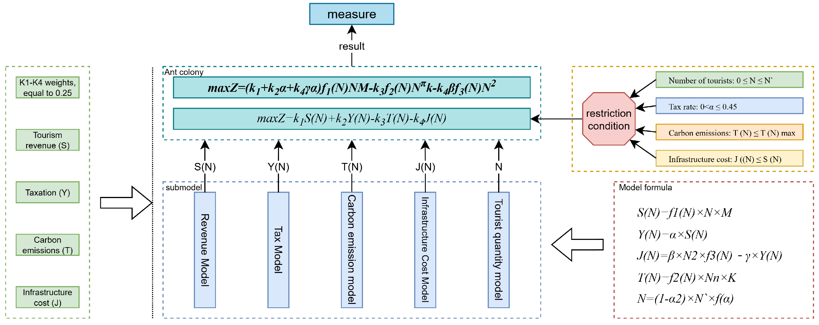
The genetic algorithm (GA) simulates the evolutionary process through selection, crossover, and mutation in order to iteratively search for the optimal solution in the solution space. The overall procedure is illustrated in
Figure 8, and the detailed steps are described as follows.
Step 1: Encoding
Each individual is represented using real-number encoding in the form of a two-dimensional vector , where N denotes the number of tourists and represents the tax rate. This encoding scheme facilitates subsequent computation and genetic operations.
Step 2: Initialization
An initial population of individuals is randomly generated within the specified constraints to ensure diversity and prevent premature convergence. For example, a population of 100 individuals may be generated, each encoded as , while satisfying all constraints.
Step 3: Fitness Evaluation
A fitness function is defined to evaluate the quality of individuals. In this study, the integrated objective function
Z serves directly as the fitness function:
Individuals with higher fitness values have a greater probability of being selected for the next generation, while ensuring that all fitness values remain positive.
Step 4: Selection
Proportional selection is employed to construct the next generation. The probability of selecting the
i-th individual is given by
where
is the fitness of the
i-th individual. Based on these probabilities, 100 new individuals are generated for the next generation, with higher-fitness individuals having a greater chance of propagation.
Step 5: Crossover
A single-point crossover operator is applied to increase genetic diversity. After selection, two adjacent individuals are chosen, and one component of their vectors is swapped. For instance, and may produce and .
Step 6: Mutation
Mutation is performed to introduce random variations and avoid premature convergence. A small perturbation is applied to one variable of a selected individual. For example, may mutate to or .
Step 7: Termination
The algorithm terminates once a predefined maximum number of iterations is reached or when the fitness values converge within a specified tolerance. At this stage, the individual with the highest fitness is regarded as the approximate optimal solution, and its encoding corresponds to the final solution of the model.
5.2.4. Results of Genetic Algorithm
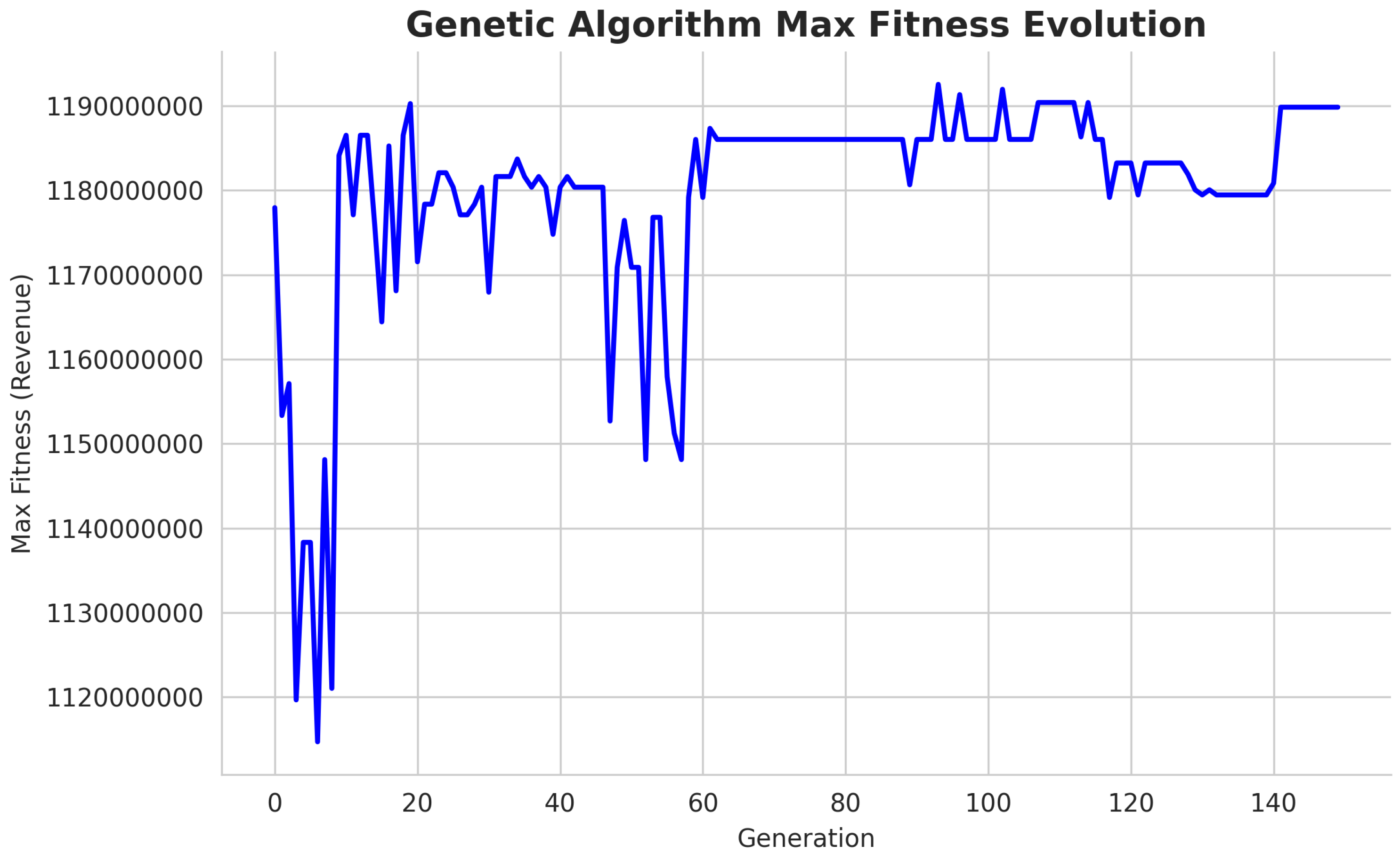
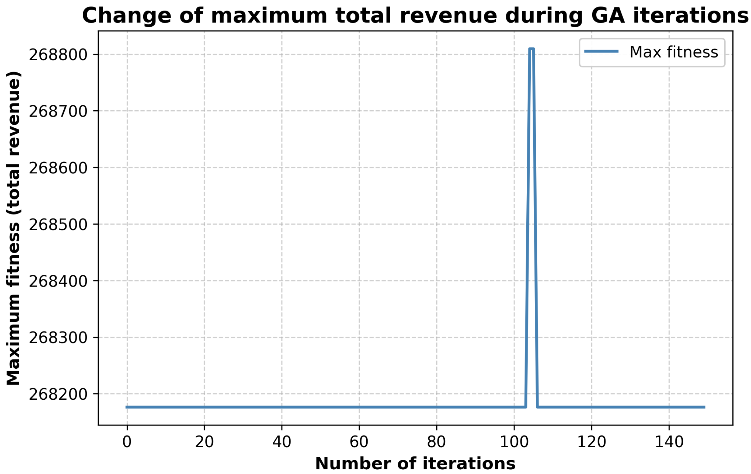
The genetic algorithm, implemented in Python3.8, iteratively optimized the comprehensive objective function. As shown in
Figure 9, fitness values fluctuated in early iterations due to stochastic operations but stabilized after ∼20 generations within
–
, confirming convergence.
The optimal solution obtained is:
Optimal number of tourists N: 196.2805 (rounded to 196)
Optimal tax rate : 0.1986
Maximum total revenue: 264,355.4569
Thus, the comprehensive optimum is approximately with .
5.2.5. Suggested Measures
To optimize the overall benefits while minimizing the environmental and infrastructural burden, the daily number of tourists should be controlled at approximately 196.
For tax regulation, the local tax rate is recommended to be maintained at around 0.198, which allows for maximizing total revenue without the adverse effects of excessive or insufficient tourist numbers.
In addition, a flexible adjustment mechanism should be established. When special environmental conditions or changes in tourist demand occur, scenic areas should appropriately and efficiently adjust both the tourist capacity and the tax rate. This ensures the achievement of comprehensive benefits while supporting the sustainable development of scenic destinations.
6. Sensitivity Analysis
In solving this model, it is not sufficient to simply apply the genetic algorithm to obtain the optimal solution. It is also necessary to verify the stability of the model by conducting sensitivity analysis. To simplify the calculation, all decimal data are rounded to integers before performing the analysis.
The procedure involves systematically adjusting the constraints to observe changes in the maximum value of the composite objective function after each variation. Specifically, once the constraints are modified, the genetic algorithm is employed to resolve the optimization problem. The results are summarized in
Table 3.
Here, denotes the fluctuation range of the upper limit of the constraint. The notation represents the change in the maximum value of the composite objective function when the upper constraint varies. R corresponds to the variables considered in the perturbation, including tax revenues, the number of tourists, and the carbon-emissions cap.
To evaluate the sensitivity between two variables, the relationship is usually represented in terms of a relative or percentage change. For instance, a
reduction in
r may result in a proportional increase in
t. Let the variation in
t be
, then the relative change of
t is expressed as
, while the percentage change is
. If
r changes by
and induces a corresponding change
in
t, the ratio of the relative changes is given by
which, in the limit
, leads to the following derivative form:
Hence, the sensitivity of
t with respect to
r is defined as the limit
Based on this definition, the sensitivity of each constraint variable with respect to the composite objective function can be systematically derived using the above sensitivity expression, and the computed values are summarized in
Table 4.
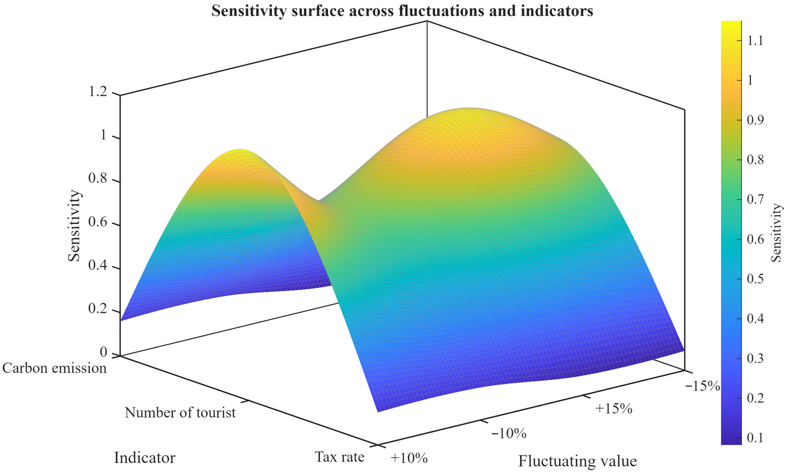
In order to transform the data in the above table into an easy-to-understand visualization and to identify the trend of sensitivity under each fluctuation, we plot the sensitivity results as a surface diagram in
Figure 10.
From
Figure 10, it is clear that tourist numbers show the highest sensitivity among all fluctuation scenarios. For instance, when the number of tourists increases by
, the elasticity
implies that the composite objective function
Z increases by approximately
. Under the same
change, the tax rate with
leads to about
change in
Z, and the carbon-emissions cap with
leads to about
change. This indicates that, compared with tax rate and carbon-emissions cap, tourist numbers exert a much stronger influence on the objective function and demonstrate greater variability. Therefore, as a key lever, controlling tourist numbers plays a decisive role in promoting sustainable development in Juneau.
7. Applicable to Other Regions
This section applies the model to Kodiak and Venice, two regions significantly affected by overtourism. The objective is to analyze the impact of regional differences on the comprehensive objective function and to identify the most critical control measures. By employing the model, less-visited areas such as Kodiak can be promoted to increase their popularity and tourism revenue, while in overcrowded destinations such as Venice, the number of tourists can be effectively controlled to avoid exceeding the maximum environmental carrying capacity, thereby supporting sustainable tourism development.
7.1. Preparation Before Model Establishment
To extend the model to two representative regions—one with a large influx of tourists and the other with comparatively fewer visitors—we first define the following variables:
: the number of tourists in the region with a high level of visitation,
: the number of tourists in the region with a low level of visitation,
: the tax rate in the region with a large number of tourists,
: the tax rate in the region with a small number of tourists.
These variables provide the foundation for constructing the optimization model.
7.2. Objective Function
To capture the trade-offs among economic, environmental, and infrastructural factors, we construct a comprehensive benefit function
Q. The optimization goal is to maximize this function, which is expressed as:
where
are weighting coefficients satisfying
. Here,
S denotes the total tourism revenues of the two regions,
Y represents the total tax revenue generated from tourism,
T is the combined carbon emissions of the two regions, and
J denotes the total infrastructure costs. This objective function balances economic benefits with environmental and infrastructural constraints, ensuring a sustainable development path.
7.3. Constraints
In order to ensure the feasibility and rationality of the optimization model, the following constraints are imposed:
Scenic Spot Capacity Constraints:
where
and
denote the maximum number of tourists that can be accommodated in the scenic spots of the two regions within a certain period. This constraint ensures that the actual number of tourists does not exceed the capacity, thereby preventing irreversible impacts caused by over-visitation.
The tax rate must remain within a reasonable range. A tax rate that is too low will reduce fiscal revenue, whereas an excessively high rate will discourage tourists and hinder the tourism market. This paper examines several major economies, including the maximum tax rates applicable in each country. The maximum tax rate is set at 45% for the purposes of this study.
Carbon Emission Constraints:
To safeguard ecological sustainability, the environmental impact of tourism should be controlled. The total carbon emissions generated by the two regions must not exceed the maximum acceptable level .
Infrastructure Cost Constraints:
Considering that the primary purpose of tourism development is profitability, the total infrastructure costs J of both regions must not surpass the total tourism revenues S.
7.4. Sub-Models
7.4.1. Revenue Calculation Model
The total revenue is assumed to exhibit a linear relationship with the number of tourists. Let the average consumption per tourist be denoted by a constant
M. Thus, the total revenue can be formulated as:
where
denotes the average expenditure of tourists in regions with a large number of visitors, and
represents the average expenditure of tourists in regions with a relatively small number of visitors.
To enhance the accuracy of the model, it is necessary to account for fluctuations in tourists’ consumption behavior due to seasonal variation, geographic location, and other external factors. Therefore, a correction factor
, defined as a function of the tourist number
N, is incorporated:
where
adjusts the revenue estimation to reflect the variability induced by changes in the number of tourists.
7.4.2. Tax Calculation Model
Since taxes are linearly correlated with the total revenue
S, the total tax can be expressed as:
where
and
denote the tax coefficients corresponding to regions with high and low tourist numbers, respectively.
7.4.3. Carbon Emission Model
Carbon emissions
T exhibit a non-linear relationship with the number of tourists
N. We therefore define the following formulation:
where
n is an exponent representing the non-linear impact of the number of tourists on carbon emissions, and
k is a constant denoting the average carbon emissions per person. To enhance the accuracy of this model, considering that
k and
n may vary due to seasonal changes and technological progress, we introduce an additional influencing factor
:
7.4.4. Infrastructure Cost Model
The infrastructure cost
J also has a non-linear relationship with the number of tourists
N, while additional revenue from taxes is invested into improving infrastructure. The model is expressed as:
where
is the infrastructure cost coefficient (usually a constant),
is the proportion of taxes allocated to infrastructure improvement, and
Y denotes the tax revenue. To improve accuracy, we further incorporate factors such as infrastructure aging and maintenance costs, revising the model as:
where
represents the degree of infrastructure aging.
7.4.5. Actual Number of Tourists Model
Changes in the tax rate lead to non-linear fluctuations in the number of tourists. Since tourists exhibit varying sensitivities to tax changes, while also being influenced by seasonal or economic cycles, the actual number of tourists is modeled as:
where
and
represent the maximum tourist capacity of the two regions within a given period, and
is the sensitivity function of tourists with respect to the tax rate.
7.4.6. Application of the Model to Venice and Kodiak
In order to further validate the effectiveness of the proposed model, we employ a genetic algorithm for optimization and apply the model to two representative regions. For the region with a large number of tourists, Venice is selected, while for the region with a small number of tourists, Kodiak is chosen. The data used in this process are obtained from public sources on the Internet. Due to space limitations, detailed data will not be listed individually.
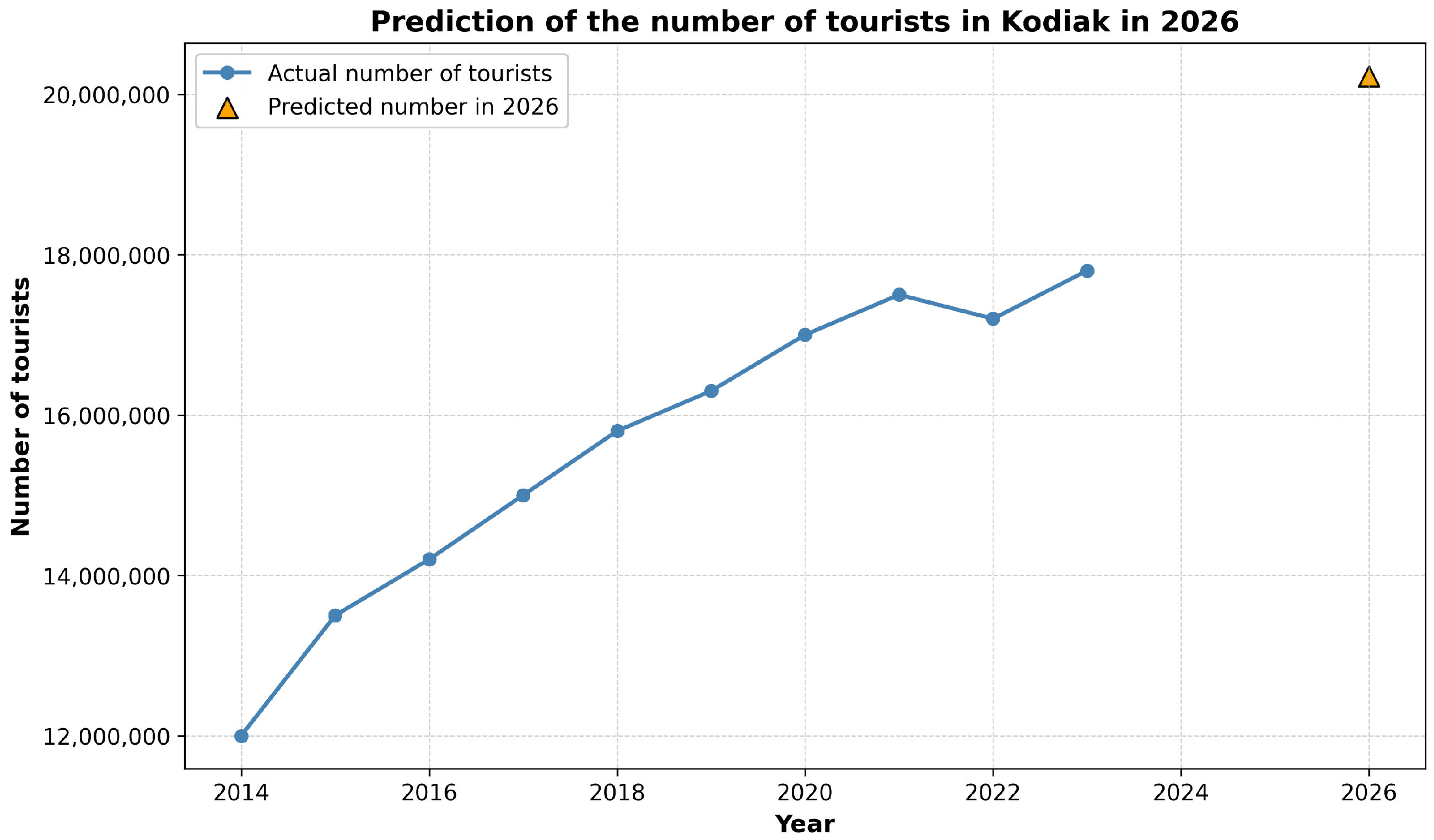
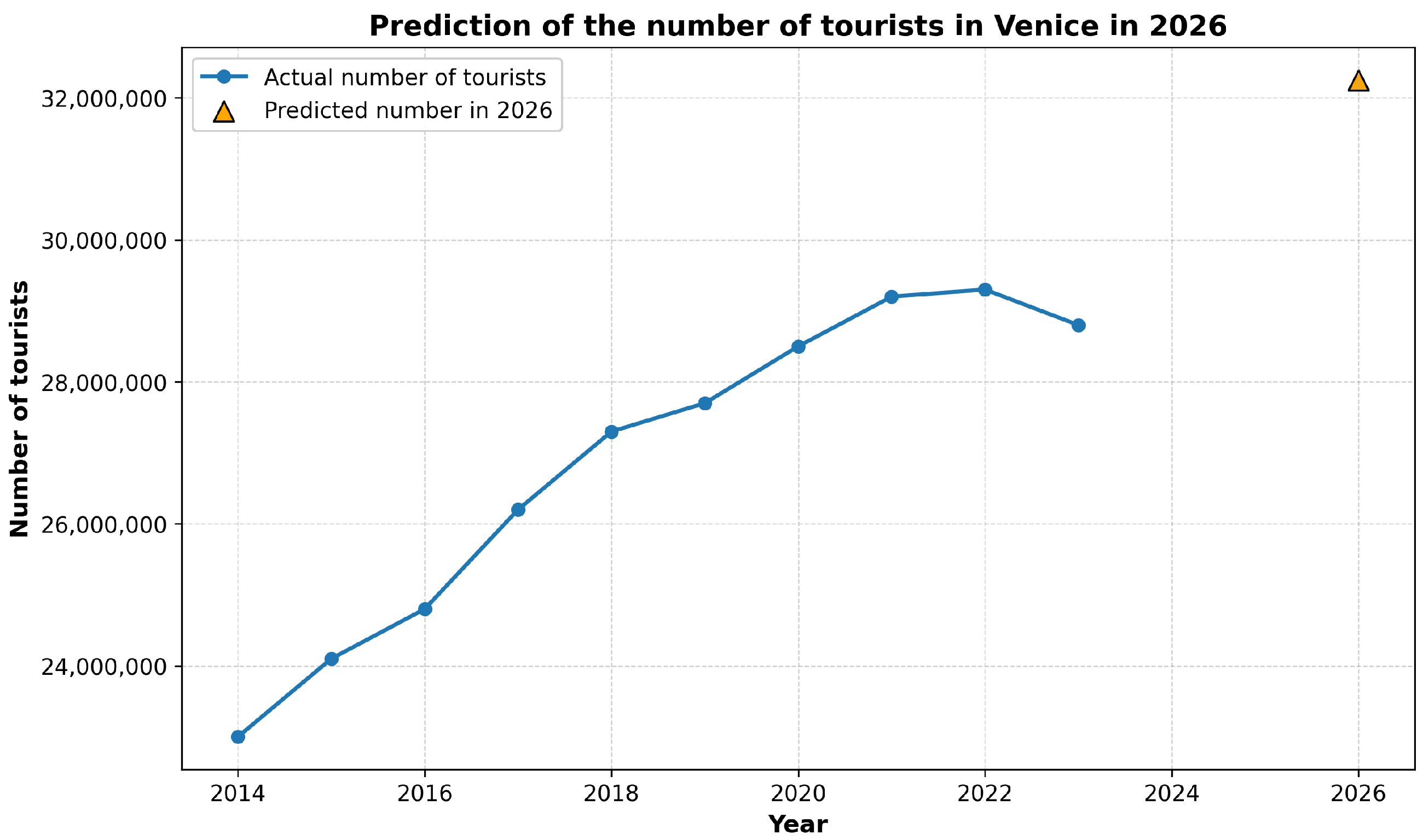
To explore the balance of tourist numbers between regions with significant differences in tourism volume, we first predict the number of tourists in Venice and Kodiak in 2026 under the natural growth trend. This provides a baseline for comparison, enabling us to later analyze whether, after implementing certain regulatory or promotional measures, the model can effectively promote tourism in regions with fewer visitors and thus achieve a better balance across regions.
The prediction results of the number of tourists in the two regions in 2026 are shown in the following
Figure 11 and
Figure 12:
7.4.7. Solution Results
Venice Region
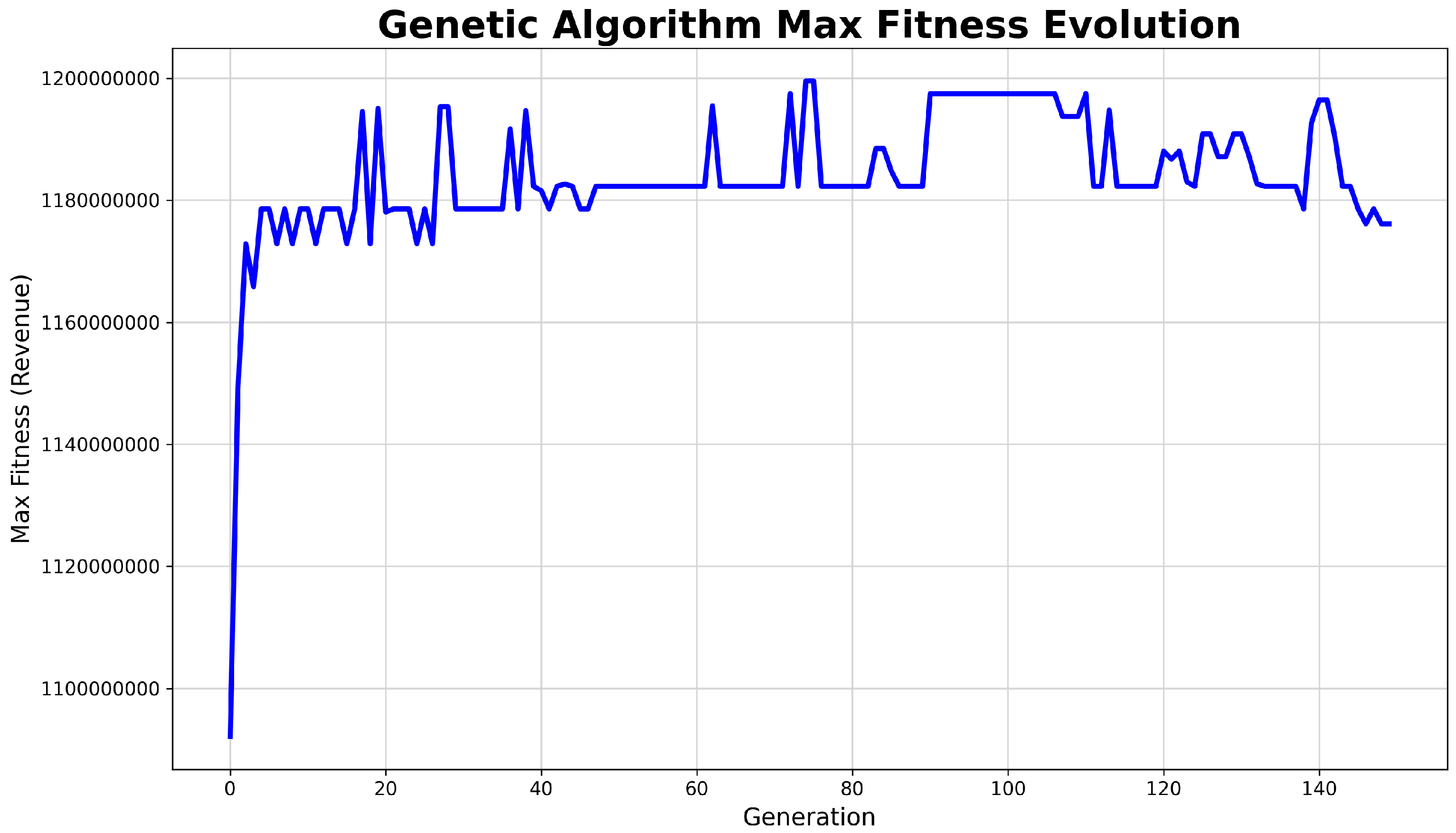
Using Python-based GA optimization, the fitness value converged after ∼40 iterations within
–
, indicating a near-optimal solution (
Figure 13). In 2026, Venice is projected to receive 32,249,090 tourists/year with 1638 t/year emissions. The optimal adjustment is 29,982,732 tourists/year with a tax rate of 0.1977, yielding maximum benefits of 1,185,337,949. This shows that regulating tourist numbers and tax rates is crucial for balancing economic and environmental goals.
Kodiak Region
Similarly, GA convergence occurred after ∼70 iterations, stabilizing within
–
(
Figure 14). In 2026, Kodiak is expected to host 20,225,454 tourists/year with 1125 t/year emissions. Optimal adjustment increases volume to 29,567,162 tourists/year with a tax rate of 0.1989, achieving maximum revenue of 1,470,921,999. Again, tourist volume and taxation emerge as decisive factors for maximizing sustainability and benefits.
7.4.8. Result Analysis
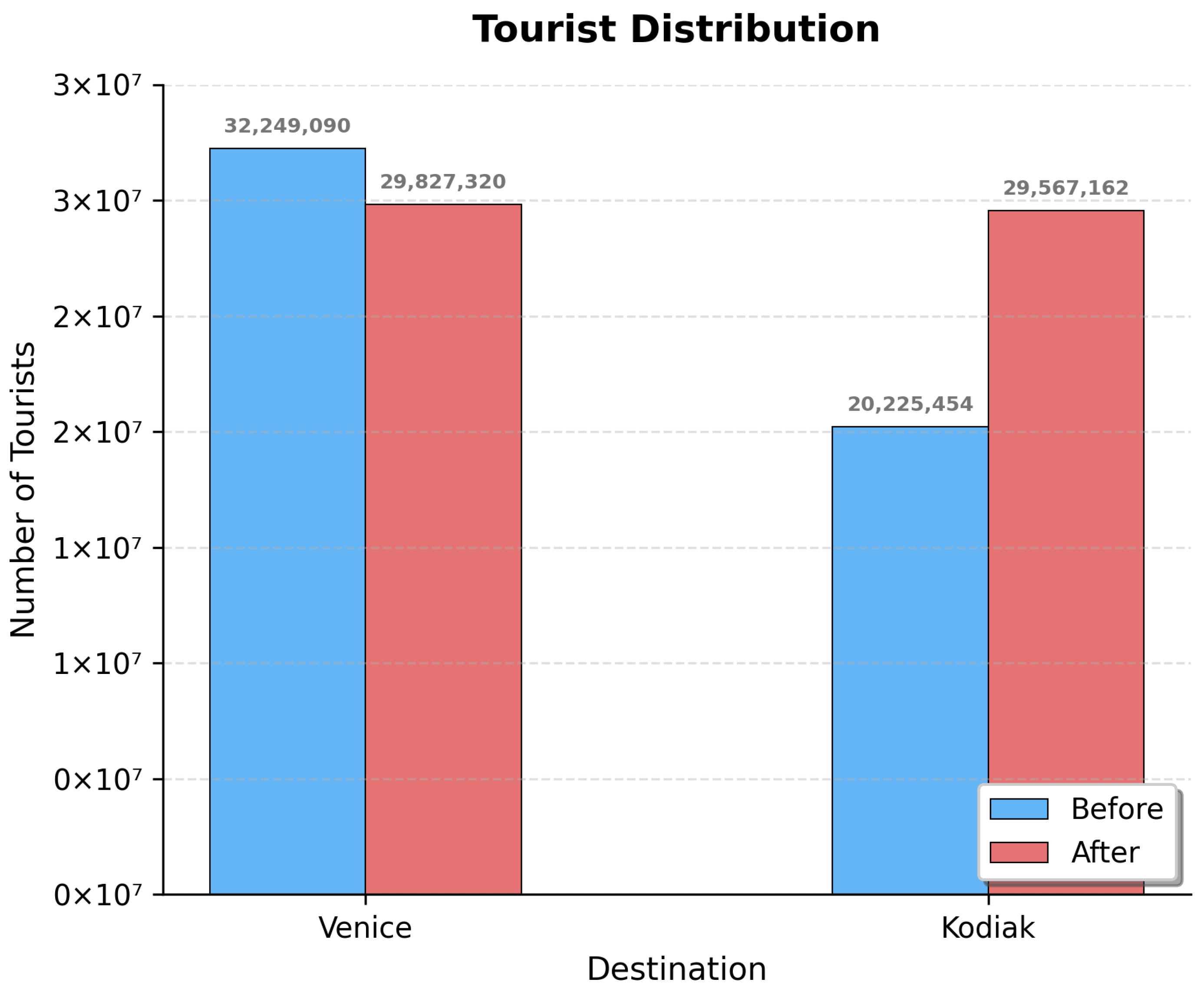
Tourist numbers and tax rates are the key factors in optimizing attractions and maximizing overall benefits, making them the primary levers for sustainable outcomes. The optimization, starting from an initial tax rate of , adjusted rates downward in both regions to enhance total benefits and balance visitor distribution. A bar chart illustrates how tax rate changes equalized tourist flows across regions.
As shown in
Figure 15, prior to the tax rate adjustment, there was a significant imbalance in the number of tourists between the two regions. After applying our model and adjusting the tax rate to the optimal value, the distribution of tourists became nearly equal, alleviating the excessive pressure on Venice while bringing greater benefits to Kodiak.
7.4.9. Suggested Measures
To regulate tourist flows, the number of visitors at attractions should be adjusted to an optimal level through a tax rate mechanism. This approach helps alleviate excessive concentration at popular destinations while encouraging more tourists to visit less-crowded sites.
For tax rate control, setting the rates of the two regions to approximately ensures a balanced distribution of tourists, preventing one region from experiencing excessive pressure.
Moreover, a dynamic adjustment mechanism should be established. In response to special environmental conditions or varying tourist demands, scenic areas should flexibly adjust both tourist numbers and tax rates. This strategy maximizes overall benefits and supports the sustainable development of tourist destinations.
8. Discussion
8.1. Verification of Hypothesis
The results of this study validate the hypothesis that the relationship between tourism growth and sustainable indicators—specifically revenue, carbon emissions, and infrastructure costs—is inherently non-linear. Unlike linear models that may overestimate carrying capacity, our multi-objective optimization framework successfully identified specific Pareto-optimal thresholds (e.g., a tax rate of for Juneau). This confirms that establishing a mathematical equilibrium between economic gain and environmental cost is essential for determining the "limits of acceptability" for a destination.
8.2. Applicability to Overtourism and Developing Destinations
The application of the model to Venice and Kodiak demonstrates its versatile applicability across destinations with distinct management needs. For Venice, a paradigmatic case of overtourism, the model functions as a restriction tool, suggesting optimal tax rates to curb excessive visitor flows while preserving revenue. In contrast, for Kodiak, the optimization results indicate that the region operates below its theoretical economic–environmental equilibrium compared to Venice; thus, the model identifies a pathway for controlled sustainable growth, allowing for an increase in visitor numbers strictly bounded by carbon emission constraints. This dichotomy proves that the proposed model is a generalized framework capable of generating tailored strategies—whether for containment or development—based on the specific carrying capacity and emission data of the destination.
9. Conclusions
This study proposes a multi-objective nonlinear optimization framework that integrates regression-based sub-models with a genetic algorithm to balance tourism revenue, tax income, carbon emissions, and infrastructure costs. By explicitly modeling threshold effects and solving for Pareto-optimal solutions, the approach identifies actionable policy levers—such as an optimal tourist volume of approximately 1.96 million and a tax rate of 0.198 for Juneau—that maximize socioeconomic benefits while respecting environmental and infrastructural constraints. The successful application to Venice and Kodiak further demonstrates the model’s adaptability across diverse tourism contexts.
Nevertheless, this work is subject to several limitations. First, the model relies on two key assumptions:
- (1)
No extreme environmental events or abnormal tourist demand shocks occur during the planning horizon.
- (2)
The policy and operational environment in Juneau remains consistent with that of 2023. While these assumptions ensure model tractability, they represent idealized conditions that may not hold under real-world volatility, such as climate disruptions, geopolitical shifts, or sudden changes in cruise industry practices. Second, the nonlinear relationships are approximated using simplified functional forms calibrated from historical data, which may overlook dynamic feedbacks or emerging behavioral patterns. Third, the genetic algorithm, though effective, is computationally intensive and sensitive to parameter settings, potentially limiting its use in real-time decision-making without further optimization.
Future research should address these gaps by incorporating stochastic or robust optimization to handle uncertainty, leveraging machine learning to capture more complex nonlinear dynamics from high-resolution data, and developing adaptive tuning strategies for metaheuristic algorithms. Expanding the framework to destinations with strong seasonality, indigenous governance, or heightened climate vulnerability would also enhance its global relevance and practical utility for sustainable tourism planning.
Author Contributions
Z.X. and X.X. contributed equally to this work and should be considered co-first authors. Z.X. was primarily responsible for conducting the core model implementation, performing extensive simulations, and drafting the initial manuscript. X.X. was responsible for the detailed study design, developing the foundational algorithm framework, interpreting the computational results, and critically revising the manuscript for intellectual content. K.Q. took charge of establishing the overall experimental design, defining the methodology for performance evaluation, and structuring the main thesis draft. W.P. and N.W. were instrumental in the subsequent validation of the model’s robustness, conducting advanced statistical data analysis, and meticulously preparing high quality figures and tables for presentation. C.C. and R.L. provided essential technical consultation, facilitated access to high performance computing resources and specialized datasets, and participated in critical discussions regarding optimization strategies. H.Q. supervised the entire project, provided critical intellectual guidance on theoretical foundations, secured necessary project funding, and was responsible for the final review and overall quality control of the manuscript. All authors have read and agreed to the published version of the manuscript.
Funding
This research received no external funding.
Institutional Review Board Statement
Not applicable.
Informed Consent Statement
Not applicable.
Data Availability Statement
Conflicts of Interest
The authors declare no conflicts of interest.
References
- Gössling, S.; Peeters, P.; Hall, C.M.; Ceron, J.-P.; Dubois, G.; Lehmann, L.V.; Scott, D.; Brajkovic, J.; Dubois, M.; Gossling, I. Tourism and water use: Supply, demand, and security. Tour. Manag. 2012, 33, 1–15. [Google Scholar] [CrossRef] [Scilit]
- Seraphin, H.; Sheeran, P.; Pilato, M. Over-tourism and the fall of Venice as a destination. J. Destin. Mark. Manag. 2018, 9, 374–376. [Google Scholar] [CrossRef] [Scilit]
- McKinley Research Group, LLC. Economic Impact of Juneau’s Cruise Industry 2023; McKinley Research Group, LLC: Juneau, AK, USA, 2024. [Google Scholar]
- McKinley Research Group, LLC. Alaska Visitor Volume Summer 2023 & Winter 2023–24; Alaska Travel Industry Association: Anchorage, AK, USA, 2024. [Google Scholar]
- Hall, C.M.; Higham, J. Tourism, climate change and the geographies of vulnerability. Tour. Geogr. 2005, 7, 331–352. [Google Scholar]
- United Nations World Tourism Organization (UNWTO). Sustainable Development of Tourism Conceptual Definition; UNWTO: Madrid, Spain, 2021. [Google Scholar]
- Sharpley, R. Tourism and sustainable development: Exploring the theoretical divide. J. Sustain. Tour. 2000, 8, 1–19. [Google Scholar] [CrossRef] [Scilit]
- Bramwell, B.; Lane, B. Critical research on the governance of tourism and sustainability. J. Sustain. Tour. 2011, 19, 411–421. [Google Scholar] [CrossRef] [Scilit]
- Li, Y.; Yang, L.; Shen, H.; Wu, Z. Urban tourism and urban change: Tourism impacts on Beijing’s hutong and courtyard housing. Tour. Geogr. 2008, 10, 453–475. [Google Scholar]
- Scott, D.; Gössling, S.; Hall, C.M. International tourism and climate change. Wiley Interdiscip. Rev. Clim. Chang. 2012, 3, 213–232. [Google Scholar] [CrossRef] [Scilit]
- Zhang, J.; Zhang, Y. Can tourism economy enhance the level of urban green development? A study based on spatial effects and threshold characteristics. J. Resour. Ecol. 2024, 15, 1094–1105. [Google Scholar] [CrossRef] [Scilit]
- Zhang, T.; Wong, W.-K.; Kilinc, O.; Alzoubi, M.A. Modeling the nonlinear impact of tourism fluctuations on green economic growth. Sustainability 2025, 24, 2540013. [Google Scholar] [CrossRef] [Scilit]
- Peeters, P.; Papp, Z. Analyzing the nexus between tourism and CO2 emissions: The role of renewable energy and R&D. Front. Environ. Sci. 2023, 11, 1257013. [Google Scholar] [CrossRef] [Scilit]
- Maggi, R.; Bertocchi, P. Anti-gravity tourism planning: An analytical approach to manage tourism congestion, seasonality and overtourism. Sustainability 2025, 17, 524. [Google Scholar]
- Hunter, C. Sustainable tourism and the touristic ecological footprint. Environ. Dev. Sustain. 2002, 4, 7–20. [Google Scholar] [CrossRef] [Scilit]
- Buckley, R. Sustainable tourism: Research and reality. Ann. Tour. Res. 2012, 39, 528–546. [Google Scholar] [CrossRef] [Scilit]
- Hunter, C. Aspects of the sustainable tourism debate from a natural resources perspective. Tour. Manag. 1995, 16, 411–423. [Google Scholar]
- Buckley, R. Ecological indicators of sustainable tourism management. Tour. Manag. 1999, 20, 51–58. [Google Scholar]
- Scott, D.; Hall, C.M.; Gössling, S. Global tourism vulnerability to climate change. Ann. Tour. Res. 2019, 77, 49–61. [Google Scholar] [CrossRef] [Scilit]
- Li, J.; Chen, X.; Li, X. Multi-objective decision making for sustainable tourism: A case study in China. J. Clean. Prod. 2018, 176, 324–339. [Google Scholar]
- Liu, Y.; Wang, E.; Li, X. System dynamics model for sustainable tourism development: A case study in China. J. Environ. Manag. 2020, 262, 110331. [Google Scholar]
- Mavrotas, G. Effective implementation of the ϵ-constraint method in multi-objective programming problems. Appl. Math. Comput. 2009, 213, 455–465. [Google Scholar]
- Nguyen, T.; Do, T.; Pham, H. Multi-objective optimization for sustainable tourism infrastructure planning. Sustainability 2019, 11. [Google Scholar]
- Lambora, A.; Gupta, K.; Chopra, K. Genetic algorithm—A literature review. In Proceedings of the 2019 International Conference on Machine Learning, Big Data, Cloud and Parallel Computing (COMITCon), Faridabad, India, 14–16 February 2019; pp. 380–384. [Google Scholar]
- Deb, K.; Sindhya, K.; Hakanen, J. Multi-objective optimization. In Decision Sciences; CRC Press: Boca Raton, FL, USA, 2016; pp. 161–200. [Google Scholar]
- Li, J.; Xu, L.; Tang, L.; Wang, S. A multi-objective optimization approach for sustainable tourism development under environmental constraints. J. Clean. Prod. 2019, 210, 233–245. [Google Scholar]
- Mavrotas, G.; Florios, K. An improved version of the augmented ϵ-constraint method (AUGMECON2) for finding the exact Pareto set in multi-objective integer programming problems. Appl. Math. Comput. 2013, 219, 9652–9669. [Google Scholar]
- Luo, Y.; Yang, L.; Tang, R. Application of genetic algorithms to optimize scenic spot tourist flow allocation. Tour. Trib. 2017, 32, 56–65. [Google Scholar]
- Kumar, S.; Singh, R. Fuzzy multi-objective programming for sustainable tourism development. Ann. Oper. Res. 2014, 227, 301–320. [Google Scholar]
- Konak, A.; Coit, D.W.; Smith, A.E. Multi-objective optimization using genetic algorithms: A tutorial. Reliab. Eng. Syst. Saf. 2006, 91, 992–1007. [Google Scholar] [CrossRef] [Scilit]
- Coello, C.A.C.; Lamont, G.B.; Van Veldhuizen, D.A. Evolutionary Algorithms for Solving Multi-Objective Problems; Springer: Berlin/Heidelberg, Germany, 2007. [Google Scholar]
- Becken, S.; Patterson, M. Measuring national carbon dioxide emissions from tourism as a key step towards achieving sustainable tourism. J. Sustain. Tour. 2006, 14, 323–338. [Google Scholar] [CrossRef] [Scilit]
- Higham, J.E.S.; Cohen, S.A. Air travel, climate change and tourism. J. Sustain. Tour. 2011, 19, 109–130. [Google Scholar]
- Dwyer, L.; Forsyth, P.; Spurr, R.; Hoque, S. Estimating the carbon footprint of Australian tourism. J. Sustain. Tour. 2010, 18, 355–376. [Google Scholar] [CrossRef] [Scilit]
- Becken, S. Operators’ perceptions of energy use and actual saving opportunities for tourism accommodation. Asia Pac. J. Tour. Res. 2013, 18, 72–91. [Google Scholar] [CrossRef] [Scilit]
- UNWTO. Indicators of Sustainable Development for Tourism Destinations: A Guidebook; World Tourism Organization: Madrid, Spain, 2004. [Google Scholar]
- Bramwell, B.; Lane, B. Sustainable tourism: An evolving global approach. J. Sustain. Tour. 2011, 19, 411–421. [Google Scholar] [CrossRef] [Scilit]
- Nguyen, T.; Jones, P.; Munday, M. Sustainable tourism infrastructure planning: A multi-objective approach. Tour. Manag. 2019, 72, 263–276. [Google Scholar]
- Mak, J.; Nishimura, E. The economics of a tourism tax earmarked for environmental protection: The case of the Hanauma Bay entrance fee. J. Travel Res. 2007, 46, 388–394. [Google Scholar]
- Garrod, B.; Fyall, A. Managing heritage tourism. Ann. Tour. Res. 2000, 27, 682–708. [Google Scholar] [CrossRef] [Scilit]
Figure 2.
3D Visualization of Tourist Numbers and Carbon Emissions Trends in Juneau.
Figure 2.
3D Visualization of Tourist Numbers and Carbon Emissions Trends in Juneau.
Figure 3.
Genetic algorithm optimization results and sensitivity analysis of key factors.
Figure 3.
Genetic algorithm optimization results and sensitivity analysis of key factors.
Figure 4.
Relationship between tourism, taxation, carbon emissions, and infrastructure cost.
Figure 4.
Relationship between tourism, taxation, carbon emissions, and infrastructure cost.
Figure 5.
Relationship between tourism, taxation, carbon emissions, and infrastructure cost.
Figure 5.
Relationship between tourism, taxation, carbon emissions, and infrastructure cost.
Figure 6.
Distribution of government fiscal expenditure across categories (unit: 104 USD).
Figure 6.
Distribution of government fiscal expenditure across categories (unit: 104 USD).
Figure 7.
Carbon Emissions Forecast in Juneau.
Figure 7.
Carbon Emissions Forecast in Juneau.
Figure 8.
Illustration of the genetic algorithm model.
Figure 8.
Illustration of the genetic algorithm model.
Figure 9.
Convergence of maximum total revenue during GA iterations.
Figure 9.
Convergence of maximum total revenue during GA iterations.
Figure 10.
Sensitivity intuitive surface plot.
Figure 10.
Sensitivity intuitive surface plot.
Figure 11.
Prediction of tourist volume in Kodiak for 2026.
Figure 11.
Prediction of tourist volume in Kodiak for 2026.
Figure 12.
Prediction of tourist volume in Venice for 2026.
Figure 12.
Prediction of tourist volume in Venice for 2026.
Figure 13.
Genetic algorithm convergence in Venice.
Figure 13.
Genetic algorithm convergence in Venice.
Figure 14.
Genetic algorithm convergence in Kodiak.
Figure 14.
Genetic algorithm convergence in Kodiak.
Figure 15.
Tourist numbers in Venice and Kodiak before and after adjustment.
Figure 15.
Tourist numbers in Venice and Kodiak before and after adjustment.
Table 1.
Notations used in this paper.
Table 1.
Notations used in this paper.
| Symbol | Description | Unit |
|---|
| N | Actual number of tourists | Ten-thousand people |
| Maximum number of tourists | Ten-thousand people |
| M | Average tourist spending | Ten-thousand US dollars |
| Total revenue | Ten-thousand US dollars |
| Total tax amount | Ten-thousand US dollars |
| Tax rate | US dollars |
| Carbon emissions | Tons |
| Infrastructure cost | US dollars |
| Weight coefficients | / |
| n | Carbon emission model exponent | / |
| k | Average per capita carbon emission | Tons/person |
| Cost coefficient | / |
| Proportion of tax revenue used to improve infrastructure | / |
Table 2.
Descriptive Statistics of Key Variables for Juneau (2019–2023).
Table 2.
Descriptive Statistics of Key Variables for Juneau (2019–2023).
| Variable | Obs | Mean | Std. Dev. | Min | Max |
|---|
| Tourist Volume (N, thousands) | 5 | 1036.5 | 672.8 | 50.0 | 1719.0 |
| Tax Revenue (Y, $ million) | 5 | 28.2 | 12.1 | 1.8 | 32.4 |
| Carbon Emissions (T, kt CO2e) | 5 | 73.9 | 14.2 | 59.7 | 92.4 |
| Infrastructure Cost (J, $ million) | 5 | 47.1 | 2.3 | 45.0 | 50.0 |
Table 3.
Descriptive statistics of dataset.
Table 3.
Descriptive statistics of dataset.
| | | Constraint Variables R |
|---|
| | Tax Revenue | Tourists | Carbon Emissions |
|---|
| +10% | 4050 | 30,282 | 4113 |
| −10% | 4050 | 21,486 | 4113 |
| +15% | 3679 | 43,099 | 3739 |
| −15% | 3679 | 34,554 | 3739 |
Table 4.
Sensitivity statistics table.
Table 4.
Sensitivity statistics table.
| | | Constraint Variables R |
|---|
| | Tax Rate α | Tourists | Carbon Emissions |
|---|
| +10% | 0.15 | 1.15 | 0.16 |
| −10% | 0.15 | 0.81 | 0.16 |
| +15% | 0.09 | 1.09 | 0.09 |
| −15% | 0.09 | 0.87 | 0.09 |
| Disclaimer/Publisher’s Note: The statements, opinions and data contained in all publications are solely those of the individual author(s) and contributor(s) and not of MDPI and/or the editor(s). MDPI and/or the editor(s) disclaim responsibility for any injury to people or property resulting from any ideas, methods, instructions or products referred to in the content. |





 ,
,