Short-Term Wind Power Prediction Model Based on SVMD-KANCNN-BiLSTM

Abstract

The large-scale integration of wind power generation, as an important sustainable energy, into the power grid relies on the support of the power system, and accurate wind power prediction is the key to ensuring the continuous and stable operation of the power system. Therefore, this paper proposes a hybrid wind power prediction model that integrates Successive Variational Mode Decomposition (SVMD) with KANCNN-BiLSTM. To address data volatility, the original wind power sequence is decomposed into seven modal components using SVMD. Subsequently, for enhanced capability in capturing nonlinear relationships, a KAN linear layer is integrated into a convolutional neural network, constructing the KANCNN-BiLSTM model for component prediction. Simultaneously, model hyperparameters are optimized via the Optuna framework to further improve predictive performance. Additionally, SHAP theory is applied to interpret the contribution of each component to the prediction results, thereby enhancing the transparency of the decomposition–integration process. Experimental results indicate that the proposed interpretable SVMD-KANCNN-BiLSTM wind power prediction model achieves a prediction accuracy of 0.998959, outperforms all comparison models across multiple evaluation metrics, and indicates superior predictive capability; additionally, the global interpretability analysis reveals that all IMF components positively contribute to the model’s predictions. The establishment of this model provides an interpretable new approach for realizing wind power prediction.

1. Introduction

Wind power generation can be said to be one of the most promising renewable energy sources. Its penetration in the global power mix is gradually increasing [1,2]. Against this backdrop, the large-scale integration of wind power into electrical grids poses considerable challenges to the operational stability, reliability and scheduling of power systems [3], while the prediction of wind power stability is pivotal to attaining this goal. Most wind power forecasting methods focus on predicting wind speed, which is then used to calculate wind power output using established models [4]. This approach has limitations, as wind speed prediction alone cannot fully capture the complex relationship between wind conditions and wind power output. It also fails to account for factors such as turbine efficiency, wind turbine characteristics [5], and environmental conditions [6]. Direct short-term wind power prediction which uses actual wind power data has gained increasing attention. This method directly forecasts power output, incorporating the real-time performance of tur-bines, leading to more accurate and reliable predictions that are crucial for operational decision-making and grid management [7,8].

Moving from physical models to statistical models [9], and recently to intelligent models, technology for predicting wind power has been constantly evolving and improving. In terms of physical models, it utilizes fluid dynamics equations and numerical weather forecasts. With the help of physical models, the relationship between wind speed and power is derived [10]. Li et al. proposed a short-term wind speed prediction method, which is based on computational fluid dynamics flow field prediction [11]. This method has the advantage of relatively strong interpretability, and high prediction accuracy. However, it has the problem of poor real-time performance and a large amount of computation. For statistical models, it relies on the use of historical data to create statistical mapping connections [12]. To evaluate the statistical wind power prediction model under uniform conditions, Manuel et al. proposed a benchmark scheme [13]. These techniques are relatively direct and their computational efficiency is also acceptable. However, they have certain obstacles in capturing nonlinear dynamic features.

Due to the strong feature extraction and pattern recognition capabilities, deep learning techniques have recently shown exceptional performance in wind power prediction. Meng et al. [14] proposed an Evolutionary Adaptive Transient Deep Learning Neural Network (EATDLNN) prediction model, combined multivariate variational modal decomposition techniques with generative adversarial networks for time series. Yin et al. [15] suggested a hybrid method for predicting wind power by using a cascaded deep learning model to extract latent meteorological and temporal data from each subsequence produced by decomposition techniques. Based on the results of feature selection, Peng et al. [16] developed a wind farm model that combined feature selection and deep learning using Bidirectional Long Short-Term Memory (BiLSTM), which provided an invaluable standard for wind power prediction in wind farm clusters.

In the early days of wind power prediction research, single neural network models were the most popular forecasting technique. However, because of the inherent instability and intermittent nature of wind energy, these single models proved insufficiently accurate in real-world applications [17]. To resolve this problem, researchers have used a “decompose-and-integrate” method. This procedure began by using a signal decomposition methodology to divide the complicated original power sequence into more regular sub-sequences, after which several prediction models were constructed for each of these sub-sequences [18]. To obtain more accurate forecast values, the prediction from each subsequence were pooled and mixed. Zhang et al. effectively modeled offshore wind generation patterns using their DWT-SARIMA-LSTM model for offshore wind power prediction [19]. Su et al. proposed a hybrid prediction system that combined Complementary Ensemble Empirical Mode Decomposition (CEEMDAN), Variational Mode Decomposition (VMD), Sample Entropy (SE), Transformers, and Gated Recurrent Units (GRU) to make ultra-short-term wind power prediction more accurate and reliable [20]. For wind power prediction, Xiong et al. developed a hybrid model that combined CEEMD, SE, RF, IRSA, BiLSTM, and ELM, attaining better prediction performance [21]; Kim et al. developed a model for predicting wind power using deep learning algorithms, thoroughly examining several deep learning techniques and input feature combinations before determining the best model architecture [22]. Nonetheless, single neural network models like Transformer and LSTM have limitations when it comes to model interpretability, hyperparameter tuning, and handling data non-stationarity.

To solve the aforementioned issues, this study proposes an explicable SVMD-KANCNN-BiLSTM wind power prediction model. The following is a summary of the main innovations and contributions:

(1) To improve the nonlinear modeling capabilities of conventional convolutional neural networks, this paper creates a KAN convolutional neural network by substituting a KAN linear layer for the CNN’s fully connected layer. This gives the network more flexibility and adaptability during the feature integration phase and serves as a foundation for developing a hybrid wind power prediction model.

(2) This research proposes an SVMD-KANCNN-BiLSTM based wind power prediction model to attain accurate wind power prediction. The wildly fluctuating raw power sequence is divided into several stable modal components by the SVMD technique. Each component is then forecasted using a KANCNN-BiLSTM model. At the same time, the Optuna framework adapts to optimize the hyperparameters of the KANCNN-BiLSTM model. It selects the optimal combination of hyperparameters to significantly improve the accuracy of the wind power prediction model.

(3) This paper introduces the SHAP theory to explain the decomposition results of SVMD since it is challenging to identify and measure the degrees of contribution of various components to the final prediction results in the current decomposition–integration framework. The decomposition–integration process is made more transparent by utilizing SHAP’s global interpretability to investigate the patterns and amounts of contribution of each IMF component to the model’s prediction outcomes. This theory provides robust backing for practical engineering applications and efficient resource distribution.

The rest of this paper is set up like this: Section 2 discusses the model framework and algorithm support. Section 3 evaluates the performance of the model through experiments and analysis. Section 4 concludes the paper and discusses directions for future research.

2. SVMD-KANCNN-BiLSTM Model Framework

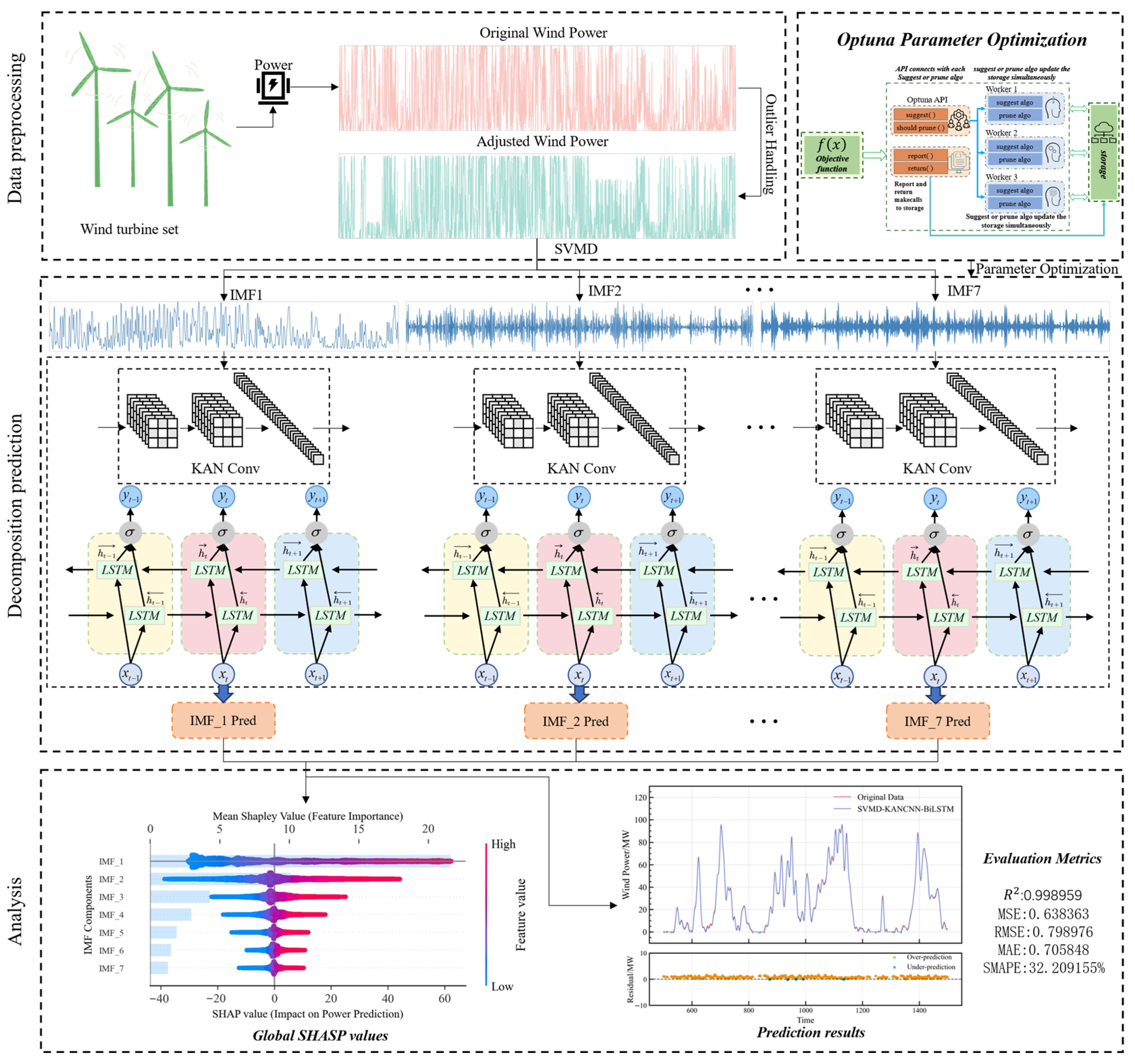
To accurately predict wind power, this paper proposes an interpretable SVMD-KANCNN-BiLSTM hybrid wind power prediction model. Three components make up this model: time series decomposition, model effect integration, and data pretreatment. Figure 1 displays the model’s schematic diagram.

The following are the model’s specific steps:

Step 1: Abnormal data less than zero should be set to zero since wind power values cannot be negative. The data is then transformed into a standard distribution with a mean of 0 and a standard deviation of 1 using the Z-score standardization technique.

Step 2: The data is broken down using the Successive Variational Modal Decomposition (SVMD) method. The ideal number of modes (K = 7) and bandwidth control parameters are found using the center frequency approach. Lastly, seven quasi-orthogonal eigenmode components (IMFs) are obtained by decomposing the original sequence.

Step 3: The Kolmogorov Arnold Network (KAN) linear layer is introduced into the convolutional neural network to construct the KANCNN-BiLSTM model for predicting each component. The KAN Convolutional Neural Network (KANCNN) module extracts spatio-temporal features from subsequences, which are subsequently processed by a bidirectional LSTM network: the forward layer captures historical temporal dependencies, while the backward layer integrates future contextual information. Dynamic temporal representations are generated through bidirectional hidden state fusion.

Step 4: Use the Optuna framework to search the KANCNN-BiLSTM model’s hyperparameter space and optimize the hyperparameters to determine the best combination.

Step 5: Use Shapley Additive Explanations (SHAP) theory to evaluate the SVMD model’s decomposition results. By utilizing SHAP’s global interpretability, you can see how each IMF component contributes to the model’s prediction results.

2.1. Algorithm Support

2.1.1. SVMD

The signal decomposition problem is converted into a global variational optimization problem via the VMD technique, which is a completely non-transitive model. The goal is to discover discrete modal components [23]. The number of modal components and the penalty factor have a significant impact on the speed of VMD [24]. Although a non-recursive method is used to address the modal overlap issue, its adaptability remains limited. Nazari M et al. introduced the SVMD approach as an extension of the VMD technique [25]. Without defining a fixed number of modal components, SVMD can continuously extract all IMFs by decomposing a signal into a series of intrinsic modal functions. Use the energy ratio and orthogonality in the mode’s frequency domain to adaptively update the two parameters. The precise solution process is outlined below:

The input signal is $f(t)$, and decompose it into two parts:

$$f(t)=u_k(t)+f_r(t)$$

(1)

where $u_k(t)$ denotes the decomposition levels of order $k$, $f_r(t)$ indicates the residual signal, which contains the unprocessed part $f_u(t)$ and the sum of the decomposition levels of order $k-1$. The calculation formula is:

$$f_r(t)={\displaystyle \sum _{i=1}^{k-1}{u}_i(t)}+f_u(t)$$

(2)

To realize the aforementioned assumptions, the following constraints must also be satisfied:

(1) The following criteria must be met in order for the decomposition sequence to include modal components with finite bandwidth focused on certain frequencies. The solution must minimize the sum of the anticipated bandwidths for all modes. Furthermore, it is bound by the requirement that the sum of all modes equal the original signal.

$$J_1={‖{\partial }_t\left[\left(\delta (t)+{\displaystyle \frac{j}{\pi t}}\right)\ast u_k(t)\right]e^{-j{\omega }_{k}t}‖}_2^2$$

(3)

where ${\omega }_k$ represents the corresponding center frequency of each mode, $k$ denotes the number of modal components, ${\partial }_t$ indicates the partial derivative of time, and $\delta (t)$ is the activation function.

(2) Another should take as many measures as possible to minimize residual signals $f_r(t)$. An adequate filter should be chosen to guarantee that this requirement may be attained steadily. The following is frequency response ${\widehat{\beta }}_k(\omega )$ and the defined constraint conditions:

$${\widehat{\beta }}_k(\omega )={\displaystyle \frac{1}{\alpha {(\omega -{\omega }_k)}^2}}$$

(4)

$$J_2={\left|\right|{\beta }_k(t)\ast f_r(t)\left|\right|}_2^2$$

(5)

where $\alpha$ denotes the penalty factor, ${\beta }_k(t)$ represents the impulse response of the filter.

(3) For the decomposition levels of order 1 to $k-1$, the corresponding process is executed. ${\beta }_i(t)$ represents the impulse response of the filter to the decomposition levels of order $i$. The following expressions give the frequency response ${\widehat{\beta }}_i(\omega )$ and the associated constraint condition:

$${\widehat{\beta }}_i(\omega )={\displaystyle \frac{1}{\alpha {(\omega -{\omega }_i)}^2}},i=1,2,\dots ,k-1$$

(6)

$$J_3={\displaystyle \sum _{i=1}^{k-1}{\Vert {\beta }_k(t)\ast u_k(t)\Vert }_2^2}$$

(7)

(4) To achieve a fully reconstructed signal, the following constraints should be added:

$$f(t)=f_r(t)+{\displaystyle \sum _{i=1}^{k-1}{u}_i(t)}$$

(8)

When the decomposition levels of order $k-1$ is known, the decomposition levels of order $k$ is:

$$\underset{u_k,{\omega }_k,f_r}{\min }\left\{\alpha J_1+J_2+J_3\right\},s.t.f(t)=u_k(t)+f_r(t)$$

(9)

The constrained variational problem is converted into an unconstrained variational problem to improve the fidelity of signal reconstruction. The augmented Lagrange function is introduced to ensure that the decomposition process effectively suppresses noise interference:

$$\begin{array}{l}L\left(\left\{u_k\right\},\left\{{\omega }_k\right\},\lambda \right)=\alpha {\displaystyle \sum _{i=1}^K{‖{\partial }_t\left[\left(\delta (t)+\frac{j}{\pi t}\right)\ast u_k(t)\right]e^{-j{\omega }_{k}t}‖}_2^2}\\ {+‖f(t)-{\displaystyle \sum _{i=1}^K{u}_k}(t)‖}_2^2+〈\lambda (t),f(t)-{\displaystyle \sum _{i=1}^K{u}_k}(t)〉\end{array}$$

(10)

where $\lambda (t)$ represents the Lagrange multiplier.

2.1.2. KAN Convolution Neural Network

(1) Kolmogorov-Arnold Network

The theoretical foundation for the KAN aims to improve on the classic Multilayer Perceptron (MLP) architecture by providing more efficient function approximation capabilities. The foundation was based on the scientific achievements of Soviet mathematicians Andrey Kolmogorov and Vladimir Arnold [22]. The MLP layer, known as the fully connected feedforward neural network, is a fundamental building block of deep learning. It is commonly used in machine learning to model nonlinear functions. A K-layer MLP neural network can be described as the interaction between the transformation matrix and the activation function. Its mathematical expression is given by:

$$MLP(\mathrm{Z})=(W_{K-1}\cdot \sigma \cdot W_{K-2}\cdot \sigma \cdots \cdots W_2\cdot \sigma \cdot W_1\cdot \sigma )\mathrm{Z}$$

(11)

The KAN neural network is a novel architecture inspired by the Kolmogorov-Arnold Representation Theorem [23]. This theorem states that for any positive integer $n$, every continuous function $f:{[0,1]}^n\to ℝ$ defined on ${[0,1]}^n$ can be represented as a finite, nested combination of one-dimensional, and continuous functions [26].

$$f(X)=f(x_1,\cdots ,x_n)={\displaystyle \sum _{i=1}^{2n+1}{\phi }_i}\left({\displaystyle \sum _{j=1}^n{\psi }_{i,j}(x_j)}\right)$$

(12)

where $f(X)$ denotes the objective function, ${\phi }_i$ is the external function, ${\psi }_{i,j}(x_j)$ represents the internal function corresponding to $j$ the external function, $X$ is the input vector and $x_j$ denotes the component of $X$.

Internal functions are used to transform input variables, providing inputs for external functions. External functions are composed of the outputs of $n$ internal functions, allowing any multivariate objective function $f(X)$ to be represented by $2n+1$ external functions. The internal function ${\psi }_{i,j}(x_j)$ of the KAN neural network is represented by the following activation function:

$${\psi }_{i,j}(x_j)=w_{1}d(x)+w_{2}spline(x)$$

(13)

where $w_1$, $w_2$ are the learning weight.

The base function $d(x)$ in the activation function is represented as:

$$d(x)=silu(x)={\displaystyle \frac{x}{1+e^{-x}}}$$

(14)

B-splines, or spline functions defined by linear combinations of basis splines, are typically used to set spline functions. This approach improves the network’s capacity to pick up complicated data representations:

$$spline(x)={\displaystyle \sum _i{c}_i{B}_i(x)}$$

(15)

where $c_i$ denotes a trainable weight coefficient.

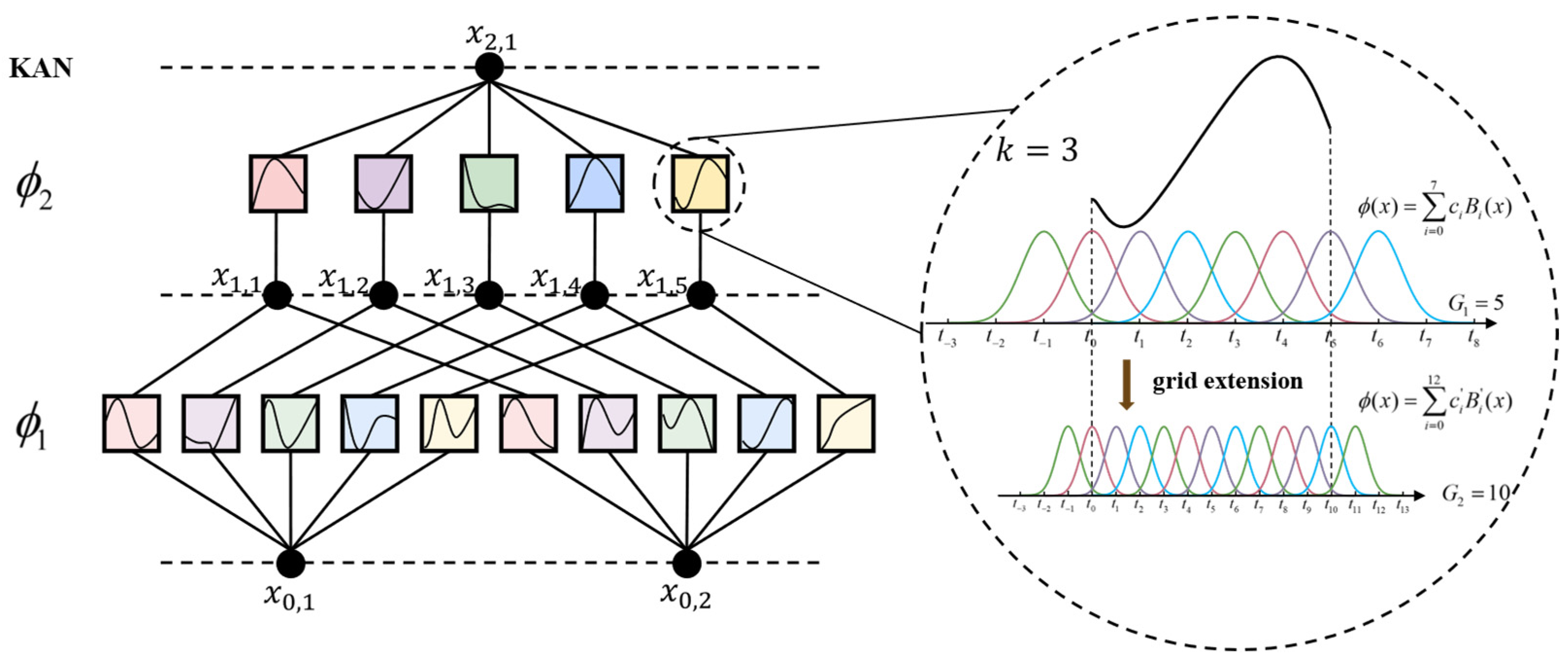
The architecture diagram of the KAN neural network is shown in Figure 2. It shares stacked layers with MLP neural networks, combining complex function mappings rather than simple linear transformations and nonlinear activations.

$$KAN(\mathrm{Z})=({\psi }_{L-1}\cdot {\psi }_{L-2}\cdots \cdots {\psi }_2\cdot {\psi }_1)\mathrm{Z}$$

(16)

The transformation ${\psi }_L$ applies to the input $x_l$ generates the next layer’s input $x_{l+1}$, which is:

$$x_{l+1}={\psi }_l(x_l)=\left(\begin{array}{ccc}{\varphi }_{l,1,1}\left(\cdot \right)& \dots & {\varphi }_{l,1,n_l}\left(\cdot \right)\\ ⋮& \ddots & ⋮\\ {\varphi }_{l,n_{l+1},1}\left(\cdot \right)& \dots & {\varphi }_{l,n_{l+1},n_l}\left(\cdot \right)\end{array}\right)x_l$$

(17)

where each activation function ${\varphi }_{l,j,i}$ serves as a spline that provides the model with a rich and adaptable response surface.

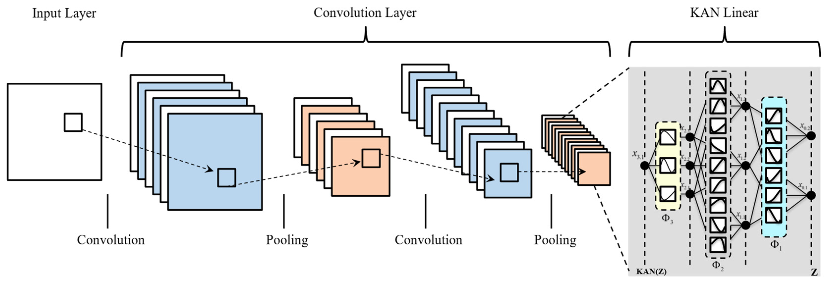
(2) KANCNN

Convolutional Neural Network (CNN) is a type of feedforward neural network that is quite frequent [27]. It has been widely employed in studies involving the learning and processing of two-dimensional data due to their ability to extract characteristics. A CNN has three main parts: convolutional layers, pooling layers, and fully connected layers. In the information processing chain, each layer serves a distinct purpose. Convolutional layers use convolutional kernels to find local features in the input data. Pooling layers keep important information by downsampling and making the process less complex. Fully connected layers combine high-dimensional features to make final predictions and classifications. During network training, the backpropagation technique is often used to optimize and update parameters [28,29,30].

This section explores methods to improve the performance of convolutional neural networks by replacing the MLP structure in fully connected layers with KAN linear layers. KAN layers use B-splines to make smooth representations of any nonlinear activation function. This means that fewer parameters are needed while still keeping the model’s expressiveness. This improvement not only enhances nonlinear modeling but also makes training more efficient and improves generalization performance to some extent. Therefore, the proposed KANCNN keeps the overall structure of classical CNNs the same, with the roles of the convolutional and pooling layers staying the same. The main distinction is the KAN modification that is used during the fully linked stage. In standard convolutions, the kernel weights are fixed and linear. In the KAN method, kernel elements are made up of learnable nonlinear functions, which gives the network more flexibility and adaptability during the feature integration phase. Figure 3 shows the KANCNN neural network design.

2.1.3. BiLSTM

One particular kind of Recurrent Neural Network (RNN) that can handle sequential data while maintaining long-term memory is called BiLSTM [31]. To overcome the drawbacks of conventional LSTMs, which only take historical data into account, BiLSTM captures bidirectional interdependence within sequences by connecting two LSTMs in opposite directions.

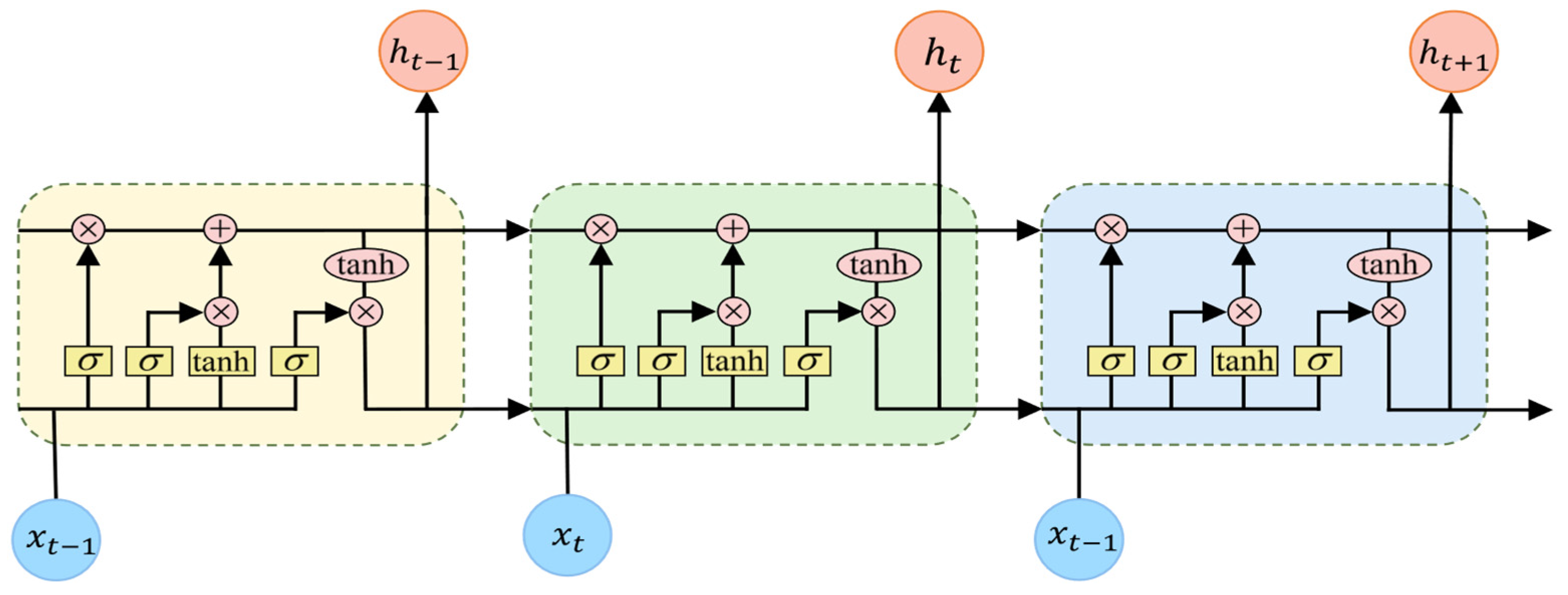
The structure of LSTM neural network is depicted in Figure 4, and its fundamental elements are the cell state and different gating mechanisms, such as the forget gate, input gate, and output gate. Because these gating methods use sigmoid functions to control information flow, LSTMs are commonly used in time-series data processing. The following is the precise computational formula for the LSTM network:

$$\left\{\begin{array}{l}{i}_t=\sigma (W_i\cdot [h_{t-1},x_t]+b_i)\\ f_t=\sigma (W_f\cdot [h_{t-1},x_t]+b_f)\\ o_t=\sigma (W_o\cdot [h_{t-1},x_t]+b_o)\\ {\tilde{C}}_t=\tanh (W_C\cdot [h_{t-1},x_t]+b_C)\\ C_t=f_t\ast C_{t-1}+i_t\ast {\tilde{C}}_t\\ h_t=o_t\ast \tanh (C_t)\end{array}\right.$$

(18)

where $i_t$ represents the input gate, $o_t$ denotes the output gate and $f_t$ is the forget gate, $\sigma$ is the sigmoid function, $\tanh$ indicates the hyperbolic tangent function, $h_{t-1}$ is the output of the memory unit at time $t-1$, and $x_t$ denotes the input to the memory unit at time $t$; $W_i$, $W_f$, $W_o$, $W_C$ are the weight vectors of $x_t$; $b_i$, $b_f$, $b_o$, $b_C$ represent the respective biases, ${\tilde{C}}_t$ indicates the candidate state of the memory unit, and $C_t$ is the state of the memory unit at time $t$.

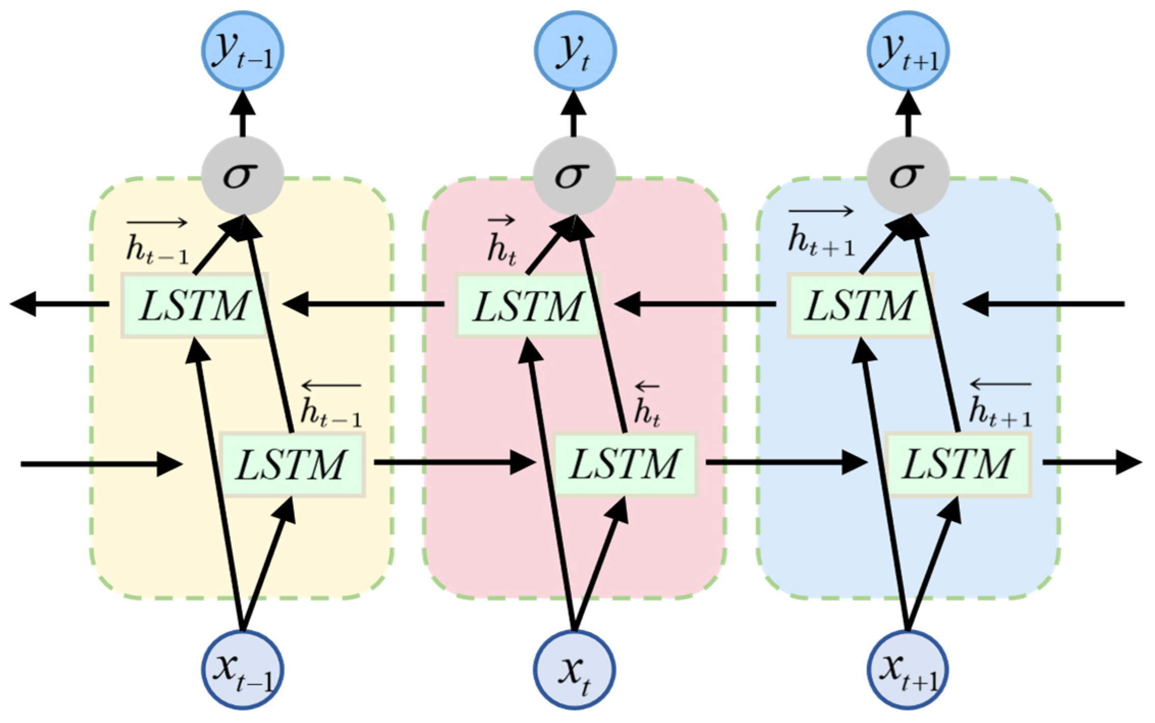
When two LSTMs analyze a time series simultaneously, one from front to back and the other from back to front. BiLSTM combines a forward LSTM and a backward LSTM [32,33,34]. Figure 5 displays its network structure. While the backward LSTM computes, the forward LSTM computes. Lastly, a new representation is created by concatenating the two outputs, as indicated by the formula below:

$$\left\{\begin{array}{l}\overrightarrow{h_t}=\mathrm{LSTM}(x_t,\overrightarrow{h_{t-1}})\\ \overleftarrow{h_t}=\mathrm{LSTM}(x_t,\overleftarrow{h_{t+1}})\\ h_t=[\overrightarrow{h_t},\overleftarrow{h_t}]\end{array}\right.$$

(19)

where $x_t$ denotes the input information at the current time step, $\overrightarrow{h_t}$ represents the hidden layer output of the forward LSTM and $\overleftarrow{h_t}$ is the hidden layer output of the backward LSTM.

2.2. Optimization Theory

2.2.1. Model Hyperparameter Optimization Method

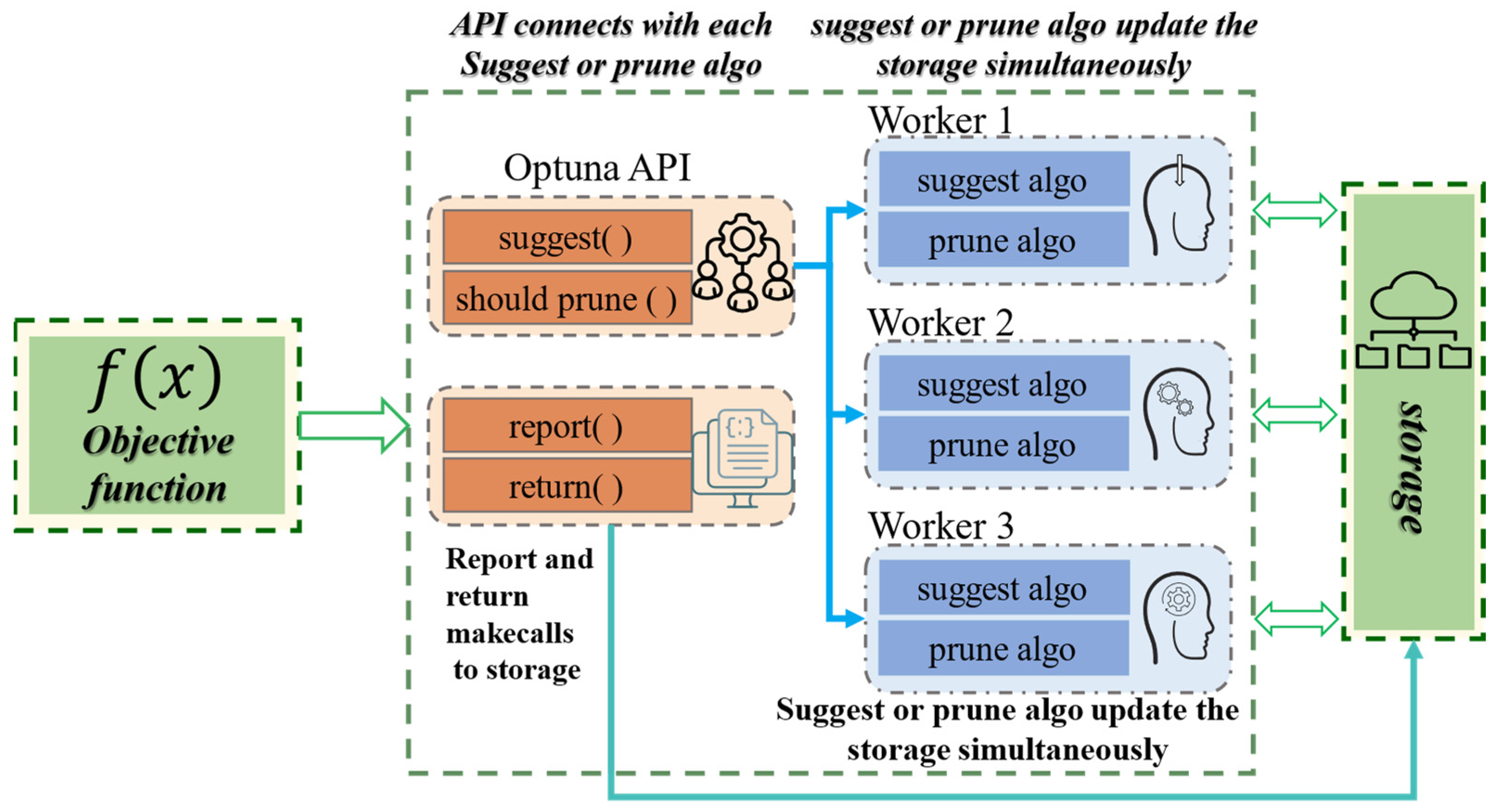
Optuna is a Python toolkit for hyperparameter optimization that can help automatically select the optimal collection of hyperparameters to improve the performance of machine learning models. Optuna supports the vast majority of machine learning frameworks, including TensorFlow, PyTorch, scikit-learn, and others (Python 3.10). Optuna utilizes Bayesian optimization techniques to explore the hyperparameter space. The Trial object, which stands for an experiment with a mix of hyperparameters, is its central component. It automatically chooses the subsequent set of hyperparameter combinations for the experiment based on the current experimental results and progressively approaches the ideal solution [35,36].

The core of the Optuna framework, as shown in Figure 6, lies in achieving a balance between efficient exploration and effective exploitation through Bayesian optimization, thereby finding the optimal hyperparameter configuration for machine learning models or algorithms.

This paper uses the Optuna framework to determine the best hyperparameters for a model, and the optimized model makes the best predictions. The exact actions to take are as follows:

Step 1: Choose the hyperparameters for the optimization.

Based on the attributes of each model module, three types of hyperparameters are carefully chosen for optimization. KANCNN used discrete search to adjust the number of convolutional kernels and the size of the pooling windows, making it easier to extract local features. This made it easier to extract local features. The number of neurons in each layer of the dual-layer BiLSTM was changed to make it better at simulating global dependencies. The nonlinear representation was improved by adjusting the number of nodes in the fully connected layer [37].

Step 2: Establish a multi-objective optimization framework.

This method employs both early stopping mechanisms and a multidimensional assessment system to determine a balance between how well the model works, how quickly it converges, and how valuable it is. This guarantees the creation of reliable and effective final models, even in situations where resources are scarce.

Step 3: Choose the optimization method and specify the search space for the hyperparameters.

In this study, Optuna’s categorical parameter is used to search for the number of convolutional kernels in the KANCNN module within the range [32, 64, 128, 256]; an integer parameter is used to optimize the pooling window size within the range [2, 8]; and Optuna’s integer parameters are used to optimize the number of neurons in two layers of the BiLSTM module independently, within the ranges 64–256 and 32–128, respectively. A joint optimization strategy is also employed to optimize the number of nodes in the fully connected layer. To efficiently explore the specified high-dimensional parameter space and ensure near-optimal hyperparameter configurations with limited computational resources, this study employs Optuna’s TPE sampling technique in combination with the Hyperband pruning strategy.

2.2.2. Decomposition Parameter Optimization Method

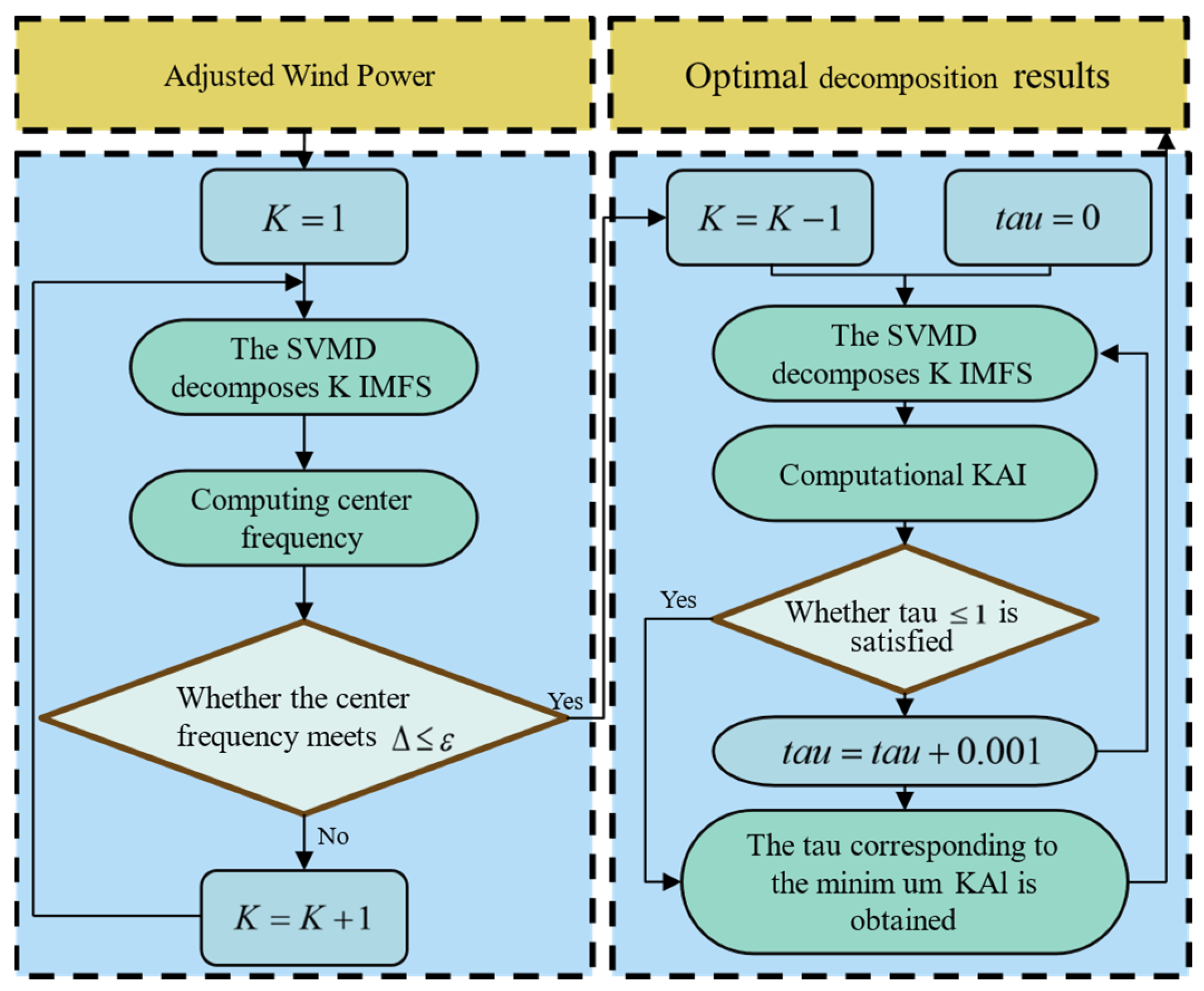
One crucial technique for determining the number of modes K in SVMD is the center frequency method. The basic concept is to achieve a balance between the requirement for decomposition and the risk of overfitting by examining how each mode’s center frequency is distributed over various K values. This method employs an iterative search approach. It begins with a smaller K number (K = 1), performs SVMD, and then logs each mode’s center frequencies. Thereafter, it gradually increases K and repeats the breakdown procedure. Each new mode typically picks up a previously unseparated frequency component in the signal when K is too low. A discernible dispersion of center frequencies across the spectrum is the result of this. By reaching a critical threshold K₀, the new mode’s center frequency approaches that of an existing mode, a phenomenon known as “mode replication. ”The center frequencies of the earlier K₀-1 modes, however, essentially remain constant across a range of K values. This means that further dissection will either produce redundant modes or fake modes rather than additional effective frequency components. Therefore, K₀-1 is the ideal number of modes since it allows you to obtain all of the major components of the signal without going too deep in the decomposition.

Compared with other decomposition parameter optimization methods, envelope entropy is often used to evaluate the purity or randomness of a single feature mode function (IMF), with the optimal IMF typically selected based on the minimum envelope entropy. For complex wind power signals, the K value corresponding to the minimum envelope entropy cannot guarantee the completeness of the overall decomposition and the degree of separation between each mode, and thus is not used as a preferred criterion. Due to the obvious volatility and noise of wind power signals, the changes in the energy difference curve are often relatively gentle and lack distinct inflection points. Therefore, determining the K value through energy difference is highly subjective and uncertain.

After establishing the optimal K, the update step parameter tau must be further optimized based on the REI metric. The following is the formula used to calculate REI:

$$REI=\min {\displaystyle \frac{1}{N}}{\displaystyle \sum _{i=1}^N\left[{\displaystyle \sum _{K=1}^K{U}_K-f}\right]}$$

(20)

where $U_K$ indicates a decomposed mode; $f$ denotes the original signal, $N$ stands for the number of signals.

Figure 7 illustrates how to update the step size parameter tau and find the best decomposition result.

Given that the value range of tau is constrained within the interval [0, 1], this study sets the iteration step size to 0.01 for global search. Based on the REI metric variation curves for different tau values, the REI metric begins to stabilize (or reach a converged state) when tau exceeds 0.18. Therefore, the optimal range for the tau parameter is defined as [0.18, 1].

2.3. Result Analysis Method

2.3.1. SHAP Theory

This study introduces the SHAP theory, which seeks to increase transparency in the decomposition–integration process. This theory also emphasizes the proportional contributions of each IMF component to the model’s forecast findings, which aids comprehension of the model’s conclusions.

SHAP is a game-theoretic approach to model interpretation that quantifies the contribution of each attribute to model predictions [38]. Compared to traditional interpretation methods, SHAP provides more granular analysis, precisely capturing local feature interactions and their specific impact on prediction outcomes [39,40]. In machine learning, the mathematical formula for SHAP values can be expressed as:

$${\varphi }_i={\displaystyle \sum }_{S\subseteq F\left\{i\right\}}{\displaystyle \frac{\left|S\right|!(g-|S|-1)!}{g!}}[f(S\cup \{i\})-f(S)]$$

(21)

where ${\varphi }_i$ represents the SHAP value for feature $i$. When the SHAP value is greater than 0, it indicates that the feature makes a positive contribution to the model’s prediction result. When the SHAP value is less than 0, it indicates that the feature makes a negative contribution to the prediction result. $g$ denotes the set containing all features, $S$ is the set excluding the feature, $f(S)$ indicates the model’s prediction value on the feature subset $S$, excluding the prediction result for feature $i$, $f(S\cup \{i\})$ is the model prediction result including the feature.

This paper explains the decision-making process of wind power prediction models using the SHAP global interpretation framework. Initially, the SHAP values for each sample in the test set are determined sequentially. The overall marginal contribution of each IMF component to the prediction outcome is then displayed using statistical aggregation. This approach determines the average strength and direction of each IMF component’s influence on power prediction at various numerical levels and offers a global ranking of feature importance. This serves as a foundation for later feature selection and model optimization while validating the model’s interpretability and logic [41,42,43].

2.3.2. Evaluation Metrics

This study uses five different error metrics—the coefficient of determination (R²) [44,45], mean squared error (MSE), root mean squared error (RMSE), and mean absolute error (MAE)-to thoroughly assess the predictive model’s performance and circumvent the drawbacks of depending just on one [46]. The following are their respective formulas:

$$R^2=1-{\displaystyle \frac{{\displaystyle \sum _{i=1}^m{\left(\widehat{u_i}-u_i\right)}^2}}{{\displaystyle \sum _{i=1}^m{\left(\overline{u_i}-u_i\right)}^2}}}$$

(22)

$$MSE={\displaystyle \frac{1}{m}}{\displaystyle \sum _{i=1}^m{\left(u_i-\widehat{u_i}\right)}^2}$$

(23)

$$RMSE=\sqrt{{\displaystyle \frac{1}{m}}{\displaystyle \sum _{i=1}^m{\left(u_i-\widehat{u_i}\right)}^2}}$$

(24)

$$MAE={\displaystyle \frac{1}{m}}{\displaystyle \sum _{i=1}^m\left|u_i-\widehat{u_i}\right|}$$

(25)

where $m$ indicates the length of the test set, $u_i$ is the actual measured value, $\widehat{u_i}$ denotes the predicted value and $\overline{u_i}$ is the mean of the actual measured values.

Each evaluation metric can undergo further normalization processing. For the R² metric, positive standardization is applied:

$${R^2}_{s,i}={\displaystyle \frac{R_i^2}{R_{\max }^2}}\times 100$$

(26)

where $R_i^2$ represents the correlation coefficient for the model, $R_{\max }^2$ is the highest correlation coefficient among all models.

For the three indicators of MSE, RMSE and MAE, negative standardization is adopted:

$$M_{s,j}=(1-{\displaystyle \frac{M_{j,i}}{M_{j,max}}})\times 100$$

(27)

where $M_{j,i}$ denotes the metric values corresponding to each model, $M_{j,max}$ represents the maximum value among all model metrics.

$$T_{s,i}={\displaystyle \sum _{i=1}^4{w}_i}\times S_{j,i}$$

(28)

where $w_i$ is the weighting assigned to each indicator, $S_{j,i}$ is the score of each indicator of each model.

3. Experiment and Analysis

To guarantee the reproducibility and engineering viability of the suggested model during experimentation, all of the tests in this study were carried out on a single computer. This computing platform includes an AMD Ryzen 9 7945HX processor (2.50 GHz, 16 cores, 32 threads), 16 GB of RAM, an NVIDIA GeForce RTX 4060 laptop GPU with 8 GB of VRAM, and 954 GB of SSD storage. The software environment comprises the Windows 10 operating system and Python 3.10 as the programming language. The main framework is TensorFlow 2.12.0. This environment guarantees the consistency and dependability of experimental results, satisfying the computational performance requirements for training and validating deep learning models.

3.1. Data Sources and Processing

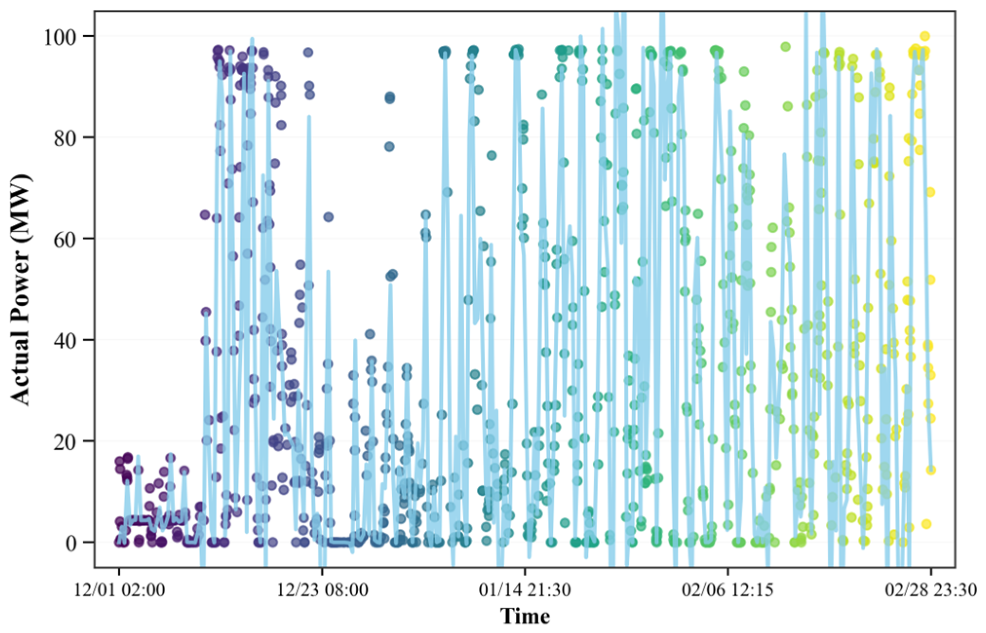
This research uses wind power production data gathered from a wind farm in Hebei Province between 2022 and 2023, with a 15 min sample interval per instance, to perform experiments. Several wind turbines are erected in real wind farms, and each one produces electricity on its own. This study considers the power-generating data from each turbine at a specific location. A training set (80%) and a test set (20%) are created from the complete dataset [47].

Figure 8 displays the actual power values from a portion of the data. Data processing is first conducted, as the collected dataset is extensive and contained a certain number of outliers. This study rigorous quality control and preprocessing for the wind power data, following this specific workflow: (1) Outlier handling: All data points below zero are considered outliers and corrected using a zero-filling technique because wind power cannot be negative; (2) Data normalization: The processed data is then converted into a standard normal distribution with a mean of zero and a standard deviation of one using the Z-score normalization method, which complies with the training requirements of deep learning models.

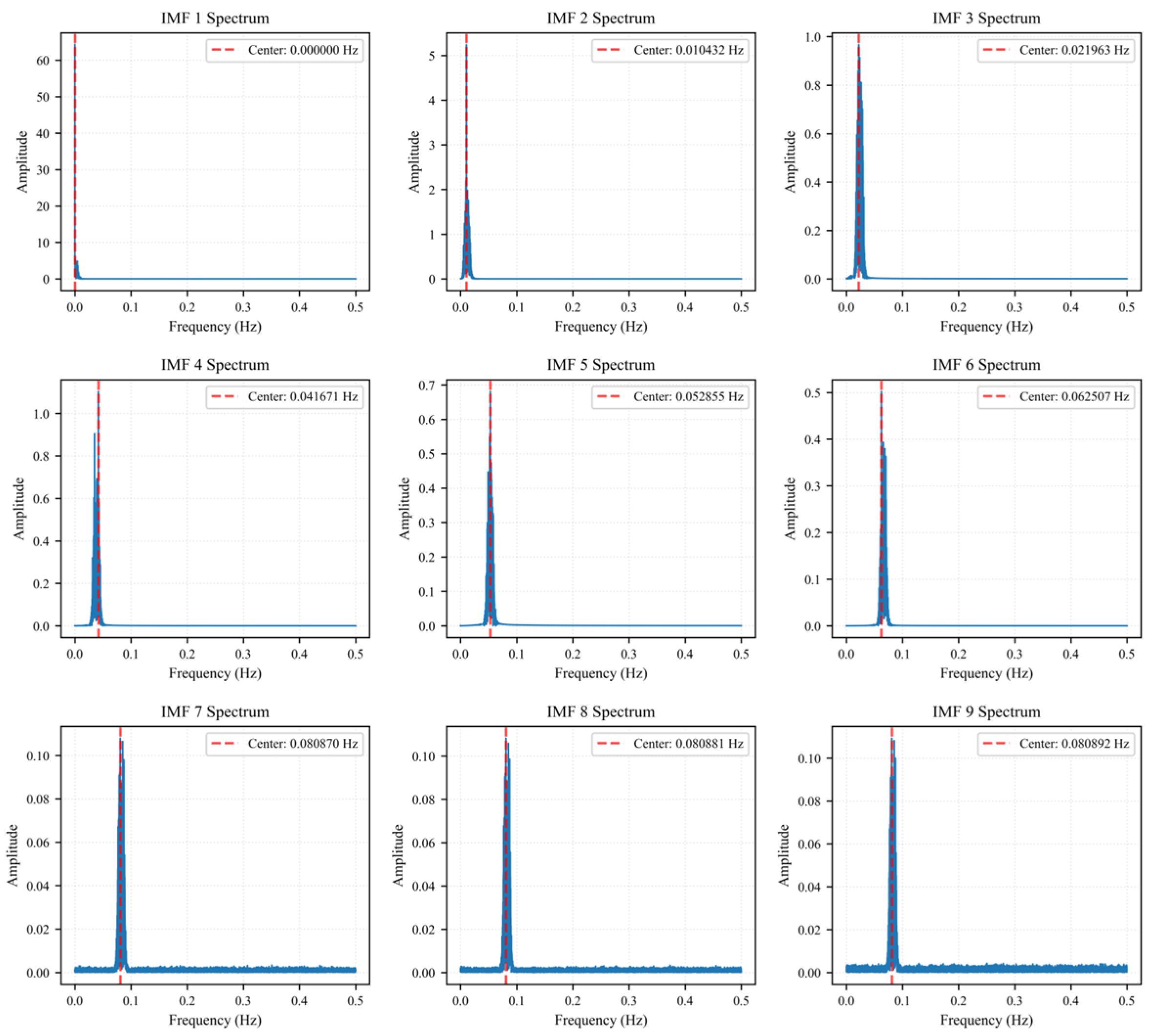
The preprocessed data is broken down using the SVMD. The starting frequency estimation technique parameter init = 1, the convergence tolerance parameter tol = 10⁻⁷, the operating frequency = 1000, and the DC component DC = 0 are the default SVMD parameters. The core parameter K for SVMD is optimized using the center frequency technique. The update step size, tau, is then determined using the residual index (REI) [48]. Figure 9 displays the computed center frequencies for each order as the modal component grows from the first to the ninth order.

When the modal component is raised to 7, the computed center frequency shows a very consistent pattern with the outcomes of an 8th-order decomposition, as can be seen by examining the change in center frequency across various K values. Continuing to increase K to 8 reveals that the model can no longer extract new, independent frequency components, indicating signs of over-decomposition. Therefore, selecting K = 7 ensures decomposition effectiveness while achieving model simplicity and efficiency. Based on this, the 7th-order (calculating by Equation (9)) decomposition is determined to be the optimal modal component value.

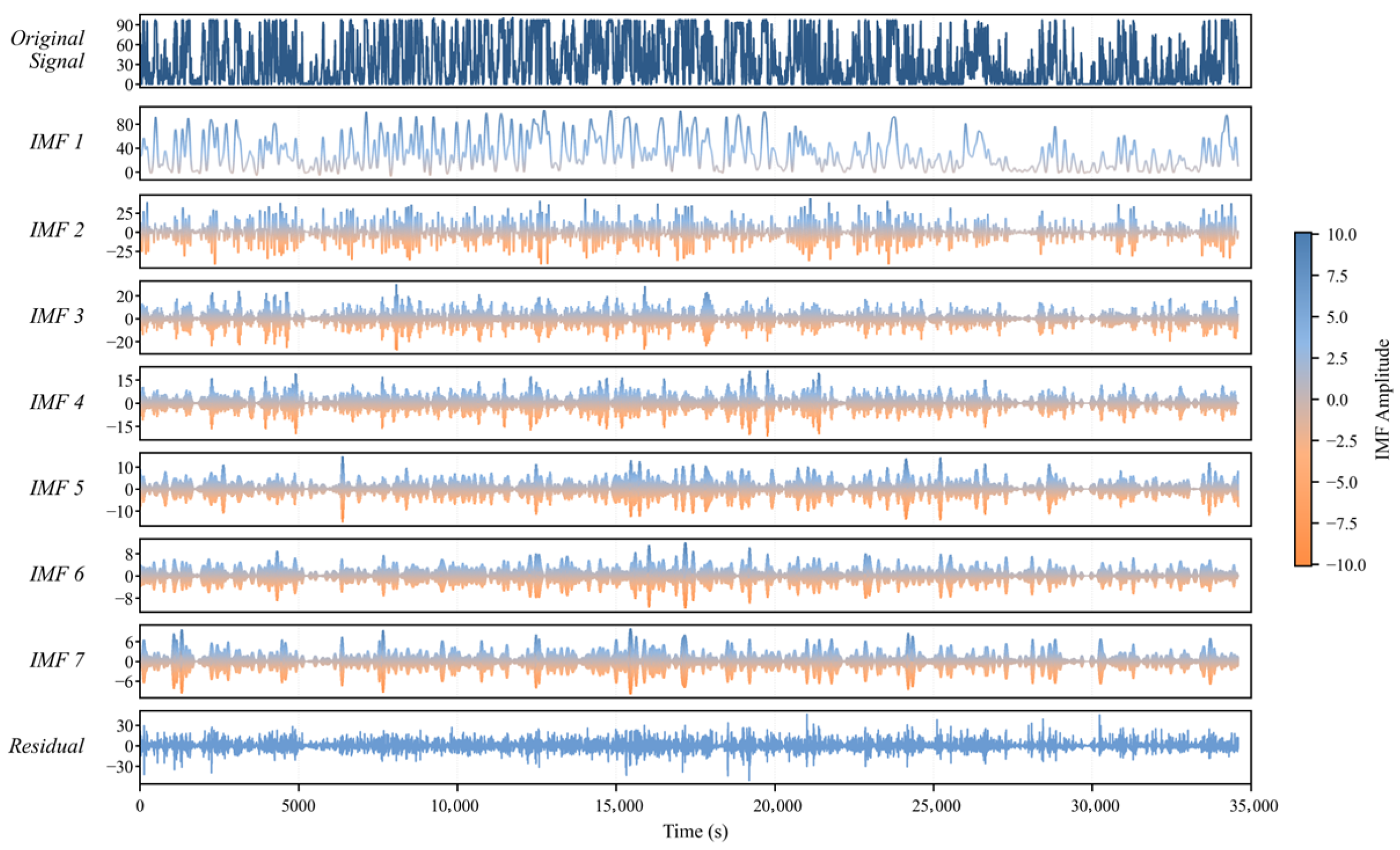
Based on the optimization results of the step size parameter for the REI indicator, the numerical inflection point is used to determine the update step size, with its set value being 0.255 (calculating by Equation (20)). The decomposition results are displayed in Figure 10 after the experimental data is simultaneously fed into the SVMD algorithm with seven decomposed modes.

Wind power time-series data is broken down into IMF1~7 using the SVMD technique from a frequency domain viewpoint. The wind power time-series dataset has several sub-signals, and as time passes, these sub-signals alter, impacting the wind power prediction model. In this study, the wind power time-series data is divided into seven sub-signals using the SVMD approach to effectively eliminate errors caused by random oscillations.

3.2. Hyperparameter Optimization for the KANCNN-BiLSTM Model

Following parameter tuning and model training based on Optuna, the core architecture and training parameter configuration of the KANCNN-BiLSTM model presented in this paper are shown in

Table 1. KANCNN-BiLSTM model Hyperparameter Optimization Table.

Module		Parameter	Value
KANCNN	Convolutional Layer	Number of convolution kernels	32
		Kernel Size	(1,1)
		Stride	(1,1)
		Pooling	1
		Kernel Size	(1,2)
	KAN Linear	Grid size	5
		Spline Order	3
		Scale Noise	0.1
		Scale Base	1
		Scale Spline	1
		Activation Function	SiLU
BiLSTM		Input Size	1
		Hidden Size 1	64
		Hidden Size 2	128
		Num Layers	2
		Output Size	1
Training hyperparameters		Epochs	50
		Patience	5
		Batch Size	256
		Learning Rate	0.001
		Optimizer	Adam

.

3.3. Analysis of Model Convergence

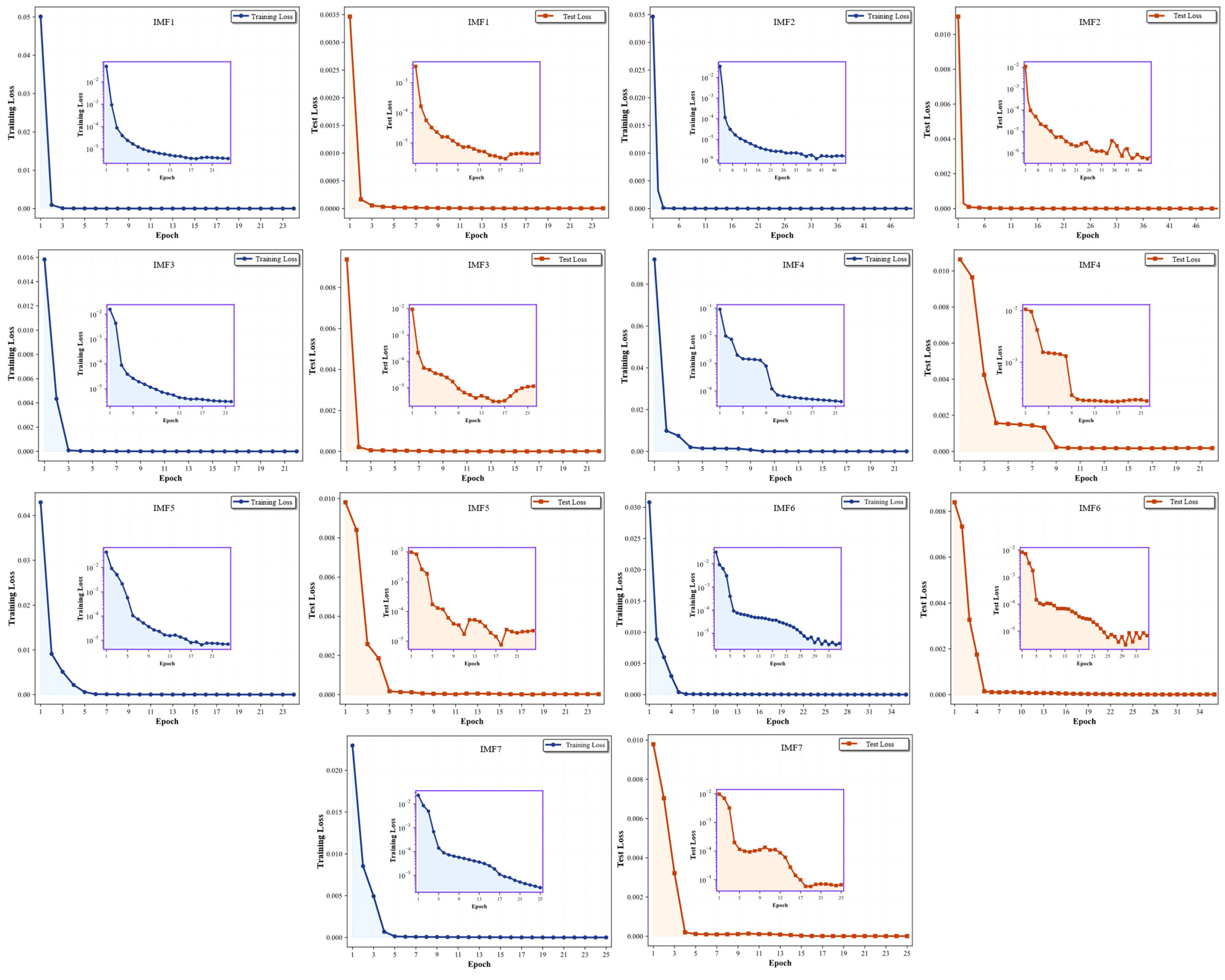
We concurrently tracked the model’s loss convergence on each eigenmode function (IMF) component training submodule in order to assess the suggested SVMD-KANCNN-BiLSTM hybrid model’s capacity for generalization and identify any instances of overfitting. Figure 11 displays the curve.

By observing the loss curves of each IMF component, it can be seen that both the training loss and the test loss can rapidly converge to a stable low value close to zero, and the convergence trajectories of the two are highly consistent without obvious divergence. This indicates that the model has achieved good generalization ability for each component, with neither underfitting nor obvious overfitting. Meanwhile, this model adopts an early stop mechanism. The early stop rule dynamically terminates training based on the performance of the test set, preventing the model from undergoing ineffective over-optimization on the training set. Therefore, the actual number of training rounds for each IMF component model is adaptively determined by this mechanism to ensure that each component stops training in the optimal generalization state.

3.4. Model Interpretability Analysis

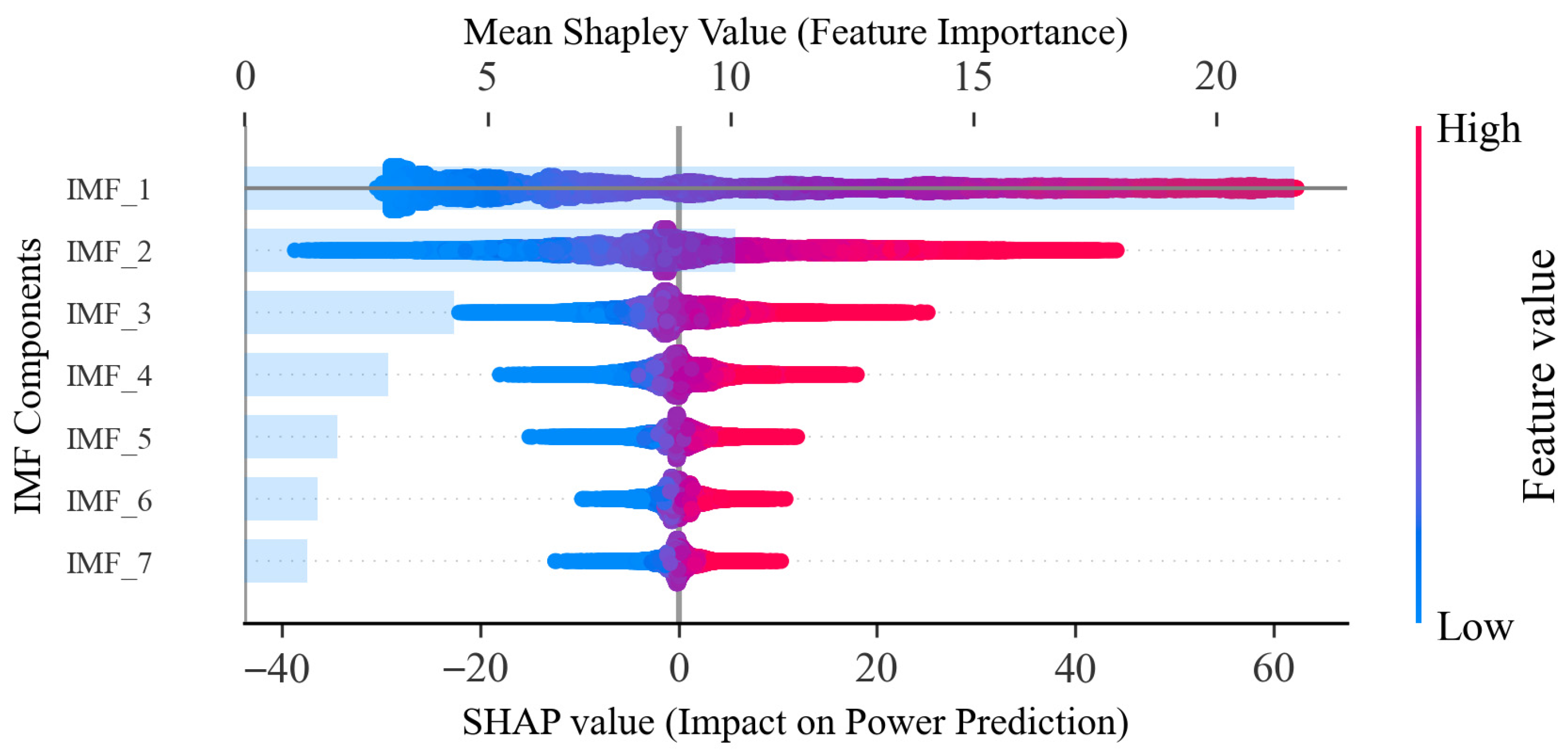
The contribution and directional influence of each IMF component on the wind power forecast output are thoroughly examined using the SHAP approach for global model interpretation. The vertical axis of the figure ranks the average absolute SHAP values of each IMF component from high to low, while the horizontal axis displays the magnitude of SHAP values, which indicate the direction and strength of a feature’s influence on forecast outcomes. Cool hues (blue) denote lower values, whereas warm hues (red) denote greater values. The feature values’ magnitude is depicted in this color mapping.

IMF_1 has the highest average absolute SHAP value, as shown in Figure 12, which indicates that it has the most impact on the model’s prediction outcomes. A strong positive contribution is shown by the fact that its high-value sample points (red) primarily cluster in the positive SHAP region, suggesting that a rise in the value of this component causes a corresponding rise in the model’s estimated wind power production. IMF_2 is the second most important. Its high-value samples are primarily found in the negative SHAP region, suggesting that raising this component has a detrimental effect by lowering the model’s estimated power output. Similarly to IMF_2, IMF_3 exhibits a distribution pattern that suggests a power suppression effect: High-value samples are associated with negative SHAP values, indicating that raising this component tends to reduce the anticipated power. IMF_4’s influence strength is marginally less than that of the previous components. The alternating positive and negative values in its SHAP distribution suggest a potentially intricate nonlinear link between this mode and wind power output. On the other hand, IMF_5 to IMF_7 exhibit lower average absolute SHAP values, with the majority of sample points clustering near zero. This suggests that these elements are comparatively insignificant in wind power prediction and have little effect on the model’s overall output.

In conclusion, SHAP theory enables a comprehensive quantification of the contribution of each IMF component to the prediction outputs. All IMF components exhibit a positive correlation with predicted outcomes, according to the result, and their contribution levels decrease from IMF1 to IMF7. This pattern provides objective explanations for identifying significant IMF components and demonstrates that various modal components of the signal are not equally essential. With the popularization of large-scale parallel computing, a computational basis has been provided for the decomposed wind power prediction model. Based on the importance of each component of the IMF analyzed by SHAP, a wind power prediction and allocation strategy for optimal resource calculation can be designed. It not only enhances the clarity of the decomposition–integration process, but also provides support for resource allocation and practical engineering applications in wind power prediction [42].

3.5. Method Comparison

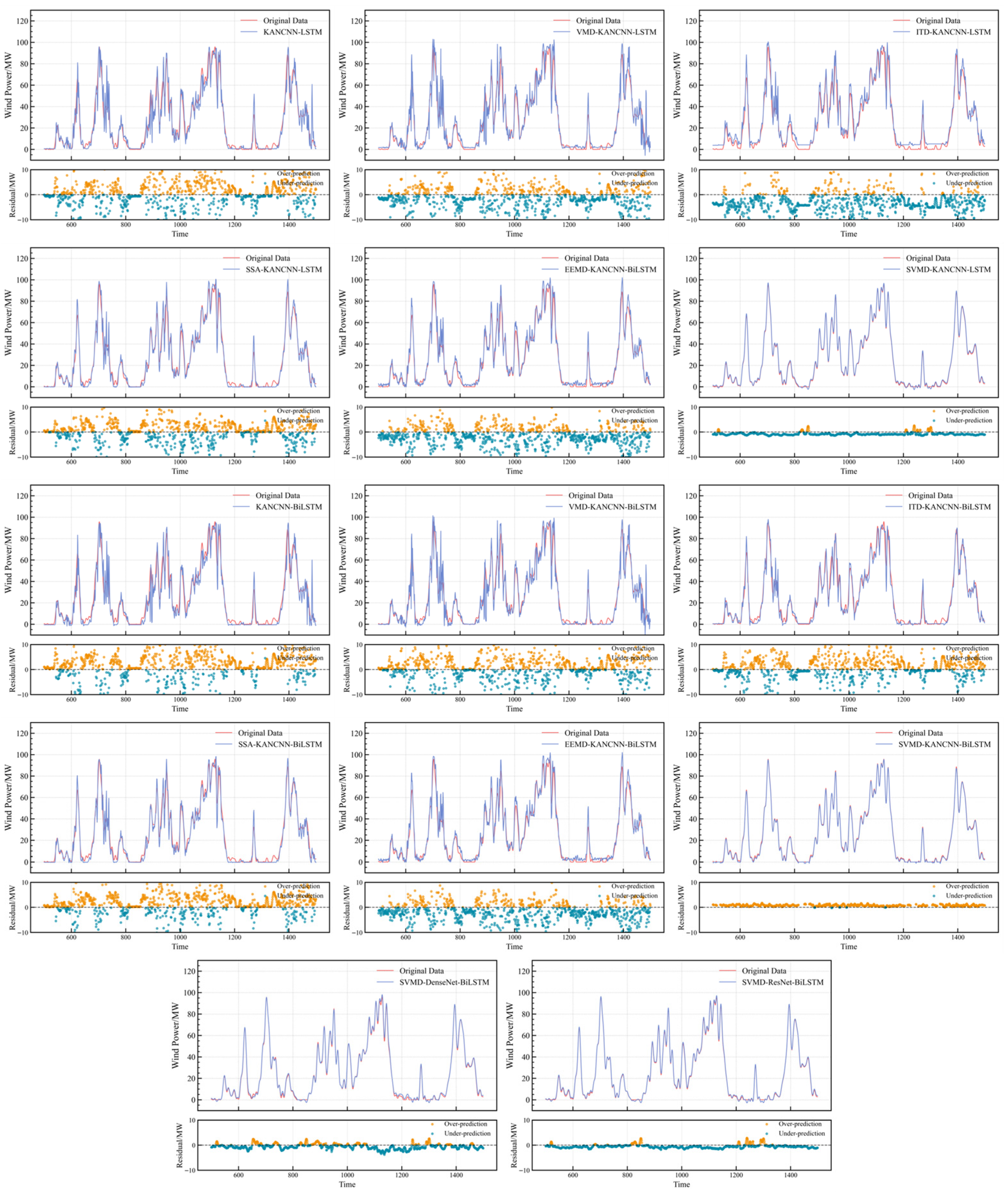
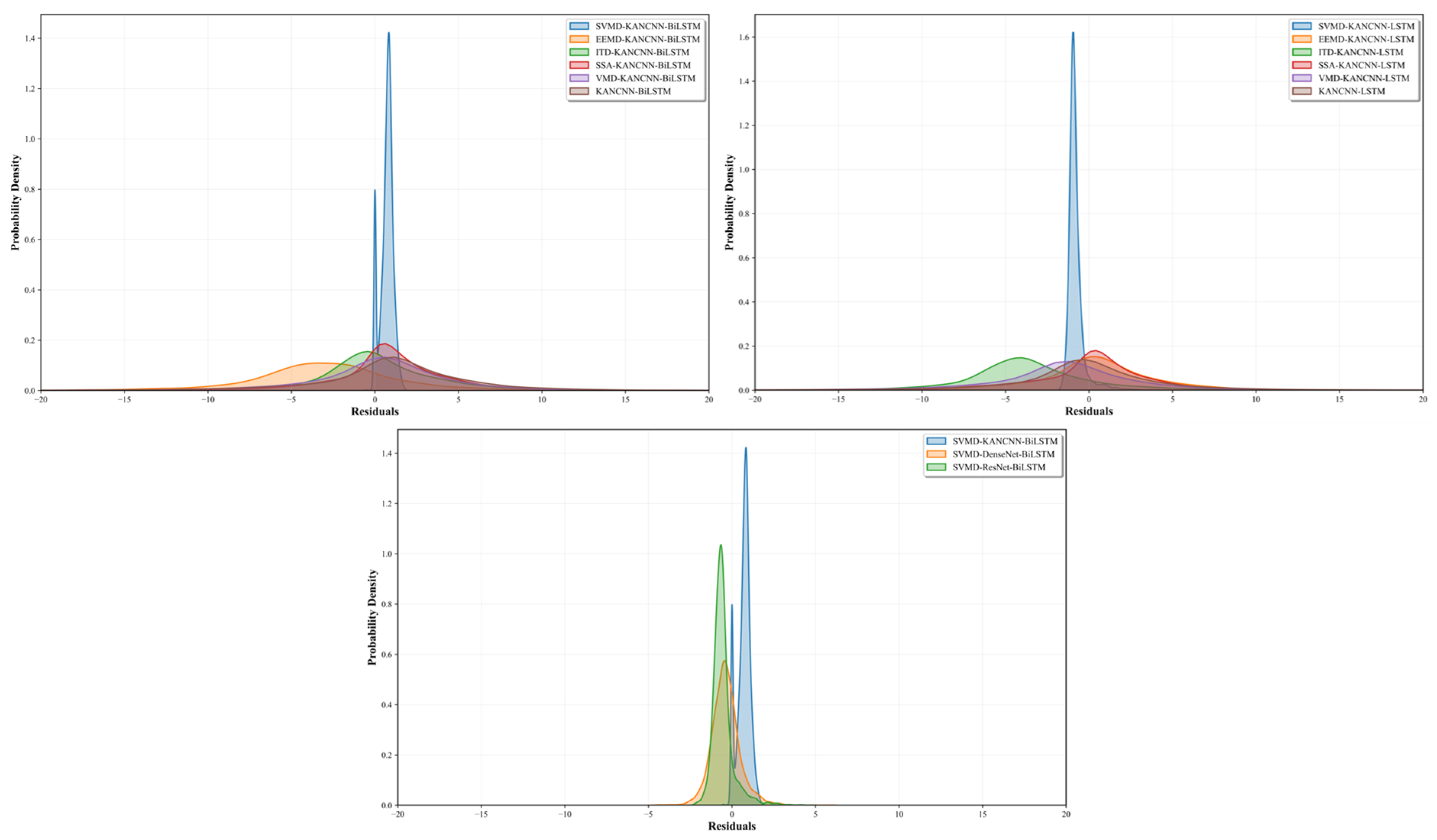
This study used a dataset of measured power data from the same wind farm that had undergone data correction to run comparative tests to thoroughly assess the overall performance of the suggested hybrid prediction of the wind power model based on SVMD-KANCNN-BiLSTM. The trials compared the proposed model to a number of benchmark approaches in two areas: prediction model architecture and signal decomposition techniques. Five decomposition algorithms, including SVMD, VMD, SSA, EEMD, and ITD, are assessed at the signal decomposition level. Several KANCNN-BiLSTM variations and KACNN variants, including KANCNN-LSTM, KANCNN-BP, KANCNN-RNN, KANCNN-MLP, ResNet-BiLSTM and DenseNet-BiLSTM are assessed at the prediction model level. The same dataset is used to train all comparison models, and on a separate prediction set, the prediction accuracy of each model is examined both quantitatively and qualitatively. This study uses similar hyperparameter setups for functionally equal modules in strict adherence to the notion of controlling variables to achieve experimental fairness. To clearly show variations in predicted performance, representative sample segments are chosen from the prediction set due to the test set’s vast scale. Figure 13 shows their prediction curves and matching residual distributions, whereas Figure 14 shows the probability density distributions of residuals across models.

The SVMD-KANCNN-BiLSTM model has the most exceptional prediction performance across all important metrics, according to this study’s thorough examination of residual data from fourteen typical hybrid models in

Table 2. Residual Comparison Analysis of Each Model.

Prediction Model	Mean Residual	Standard Deviation	Standard Error	95% CI	100% CI
SVMD-KANCNN-BiLSTM	0.7046	0.3767	0.0045	[0.6957, 0.7135]	[−0.5445, 1.9164]
SSA-KANCNN-BiLSTM	0.7330	4.1513	0.0500	[0.6347, 0.8311]	[−36.7890, 26.2099]
ITD-KANCNN-BiLSTM	0.0684	4.2178	0.0508	[−0.0312, 0.1681]	[−34.1603, 35.1380]
EEMD-KANCNN-BiLSTM	−3.2245	4.6273	0.0558	[−3.3339, −3.1152]	[−45.1030, 17.2969]
VMD-KANCNN-BiLSTM	−0.1976	7.4439	0.0897	[−0.3735, −0.0217]	[−81.7701, 69.4102]
KANCNN-BiLSTM	0.7466	7.0937	0.0855	[0.5790, 0.9143]	[−74.8312, 60.6196]
SVMD-KANCNN-LSTM	−0.7932	0.5251	0.0063	[−0.8056, −0.7808]	[−1.6990, 5.1407]
EEMD-KANCNN-LSTM	0.0961	4.1962	0.0506	[−0.0031, 0.1952]	[−42.0137, 20.4195]
SSA-KANCNN-LSTM	−0.2215	4.3319	0.0522	[−0.3238, −0.1191]	[−37.5093, 22.9843]
ITD-KANCNN-LSTM	−3.8341	4.3824	0.0528	[−3.9376, −3.7305]	[−41.4643, 28.6018]
VMD-KANCNN-LSTM	−2.1020	7.5705	0.0913	[−2.2809, −1.9232]	[−85.2807, 67.5681]
KANCNN-LSTM	−0.5957	7.4524	0.0898	[−0.7718, −0.4196]	[−75.8344, 57.4949]
SVMD-DenseNet-BiLSTM	−0.3713	0.5104	0.0204	[−0.3918, −0.3509]	[−4.4618, 5.8022]
SVMD-ResNet-BiLSTM	−0.5560	0.6475	0.0178	[−0.5713, −0.5407]	[−2.2984, 4.7633]

. With a residual standard deviation of just 0.3767, this model shows remarkably outstanding prediction stability compared to other comparable models. At the same time, its 0.0045 standard error is the lowest of all models, indicating the best level of parameter estimation accuracy. This model has the lowest 95% CI [0.6957, 0.7135], indicating strong statistical reliability, despite somewhat systematic overestimation (mean residual of 0.7046). Overall, SVMD series models outperform other signal decomposition methods. The SVMD-KANCNN-LSTM model has strong prediction stability but suffers from systematic underestimation, whereas the SVMD-KANCNN-BiLSTM model has the best overall performance. In terms of neural network designs, BiLSTM models performed better than their LSTM counterparts in most cases, with the greatest gain seen when SVMD is added. Other hybrid models, such as ITD-KANCNN-BiLSTM and EEMD-KANCNN-LSTM, have higher unbiasedness but worse predictive consistency. Both the basic KANCNN model and the VMD-based models exhibit strong volatility and bias. After careful consideration of statistical properties, reliability, and predictive accuracy, SVMD-KANCNN-BiLSTM is chosen to be the best prediction model. This conclusion is an essential point of reference for choosing a model for challenging time series forecasts.

This study uses R², MSE, RMSE, and MAE (calculating by Equations (22)–(25)) as assessment measures to further analyze model performance.

Table 3. Comparison of Model Evaluation Metrics.

Method	R2	MSE	RMSE	MAE
SVMD-KANCNN-BiLSTM	0.998959	0.6383	0.7989	0.7058
SSA-KANCNN-BiLSTM	0.971020	17.7681	4.2152	2.8193
ITD-KANCNN-BiLSTM	0.970982	17.7916	4.2180	2.8422
EEMD-KANCNN-BiLSTM	0.948124	31.8059	5.6396	4.3145
KANCNN-BiLSTM	0.917030	50.8702	7.1323	4.0953
VMD-KANCNN-BiLSTM	0.909572	55.4431	7.4460	3.7540
SVMD-KANCNN-LSTM	0.998524	0.9050	0.9513	0.8939
EEMD-KANCNN-LSTM	0.971271	17.6145	4.1967	2.8706
SSA-KANCNN-LSTM	0.969317	18.8121	4.3373	2.8514
ITD-KANCNN-LSTM	0.944704	33.9026	5.8226	4.7009
KANCNN-LSTM	0.916999	55.8845	7.4756	3.8708
VMD-KANCNN-LSTM	0.899330	61.7225	7.8564	4.1669
SVMD-DenseNet-BiLSTM	0.988552	0.8880	0.9423	0.7981
SVMD-ResNet-BiLSTM	0.992812	0.7885	0.8534	0.7899

shows that the hybrid model for predicting wind power based on SVMD-KANCNN-BiLSTM outperformed all other comparison models. The R² value is 0.998959, with the lowest MSE, RMSE, and MAE values of 0.6383, 0.7989, and 0.7058, respectively. This suggests that the model has the highest prediction accuracy and outstanding fitting capability. Compared to the KANCNN-LSTM model, the KANCNN-BiLSTM model improves R² by 0.000031, while decreasing MSE and RMSE by 5.0143 and 0.3433, respectively. Compared with the CNN variant models SVMD-DenseNet-BiLSTM and SVMD-ResNet-BiLSTM, the R² of the SVMD-KANCNN-BiLSTM model has increased by 0.010407 and 0.006147. MSE and RMSE decreased by 0.2497, 0.1502, 0.0923 and 0.0841, respectively. The KANCNN-LSTM model, which uses SVMD, has adequate accuracy, although R² is somewhat lower (0.998524) and other error metrics are greater. This statistic further demonstrates the superiority of the BiLSTM structure for gathering time series information about bidirectional interdependence. Furthermore, all decomposed models perform much better than the baseline models (KANCNN-BiLSTM and KANCNN-LSTM), which do not use physical integration and signal decomposition approaches. This data shows how the decomposition–integration method significantly reduces non-stationarity in wind power sequences, increasing the accuracy of feature extraction and pattern recognition.

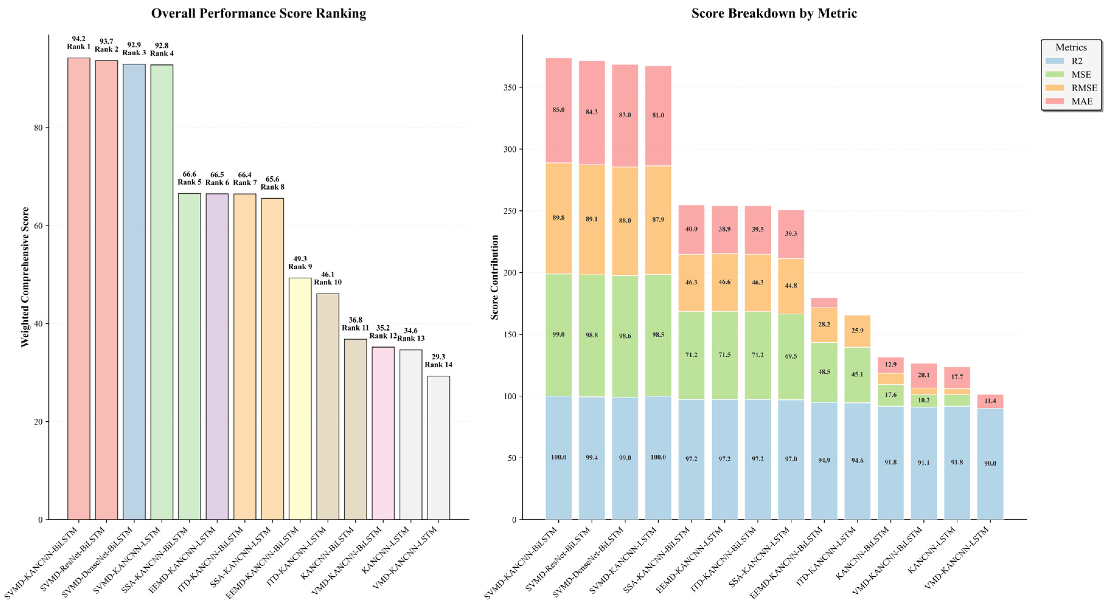
This study normalizes each evaluation indicator and turns them into percentage-scale scores to further demonstrate the model’s accuracy. As Figure 15 shows, positive standardization is used for the R² statistic, while negative standardization is used for the MSE, RMSE, and MAE metrics. Finally, a weighted sum technique with the following weight distribution is used to obtain the comprehensive score: MAE (20%), MSE (25%), RMSE (25%), and R² (30%) (calculating by Equations (26) and (27)). Each model’s comprehensive scores are acquired (calculating by Equation (28)), and illustrates how the models are rated in relation to these scores. A higher score indicates better overall model performance.

In conclusion, the SVMD-KANCNN-BiLSTM based interpretable wind power prediction model performs better than alternative models in terms of overall prediction accuracy, stability, and generalization ability. It validates the superiority of the model that combines the SVMD approach with the KAN convolutional neural network and BiLSTM in the prediction of wind power by achieving the best R² value and the lowest error rate.

To verify the significant performance differences between the SVMD-KANCNN-BiLSTM wind power prediction model and other comparison models, this paper conducts pairwise tests on the proposed model and 13 comparison models on the test set. The mean based t-test and the variance based Levene test were, respectively, used.

Table 4. Statistical significance test results.

Comparative Model	t Test p Value	Levene Test p Value
SSA-KANCNN-BiLSTM	0.00	0.00
ITD-KANCNN-BiLSTM	0.00	0.00
EEMD-KANCNN-BiLSTM	0.00	0.00
KANCNN-BiLSTM	0.00	0.00
VMD-KANCNN-BiLSTM	1.66 × 10−304	2.16 × 10−286
SVMD-KANCNN-LSTM	6.87 × 10−210	2.64 × 10−56
EEMD-KANCNN-LSTM	0.00	0.00
SSA-KANCNN-LSTM	0.00	0.00
ITD-KANCNN-LSTM	0.00	0.00
KANCNN-LSTM	0.00	0.00
VMD-KANCNN-LSTM	0.00	7.44 × 10−269
SVMD-ResNetT-BiLSTM	0.00	0.00
SVMD-DenseNet-BiLSTM	8.90 × 10−3	3.91 × 10−144

shows the outcomes.

According to the results of the t-test and Levene test, the SVMD-KANCNN-BiLSTM model has significant differences from other comparison models. Because its performance indicators are all superior to those of other models, the model proposed in this paper is significantly better than all the comparison models.

Furthermore, this study compares the training timeframes needed for various models and examines model complexity in light of the aforementioned findings:

As shown in

Table 5. Model Runtime Comparison.

Data Processing Method	KANCNN-LSTM	KANCNN-BiLSTM
Do not Decomposition	58 s	69 s
EEMD	66 s	74 s
ITD	178 s	208 s
SSA	145 s	382 s
VMD	76 s	124 s
SVMD	37 s	49 s

, the time complexity of the proposed SVMD-KANCNN-BiLSTM hybrid wind power prediction model is primarily influenced by data preprocessing, model training, prediction, and result integration stages. Therefore, the polynomial time complexity is $O(f(l,V,a,b,r,p,q))$, where $l$ denotes the sample size, $V$ indicates the number of training iterations, and $a$ represents the number of training samples, $b$ is the parameters within the model and $r$ denotes the number of prediction samples, while $p$ and $q$ represent the dimension and length of data in the ensemble phase. As can be seen from the above, the number of iterations in the training phase, the scale of the data, and the number of model parameters $(V,a,b)$ dominate the overall time complexity. After introducing SVMD, although the data is decomposed into multiple submodal signals, increasing the data volume, this method exhibits high parallelism and convergence. It enables parallel training and prediction of multiple sub-signals with the support of modern computational hardware. Therefore, the overall training time is primarily composed of the longest single sub-signal training time and the overhead of the decomposition and integration process. It can be expressed as: $T_t\approx T_{SVMD}+\max (T_{t,i})+T_e$, where $T_{SVMD}$ denotes the SVMD time, $T_{t,i}$ denotes the training time, and $T_e$ denotes the ensemble phase time.

Table 3 and Table 5 demonstrate that SVMD maintains satisfactory prediction accuracy while achieving greater computing efficiency. In addition to showing better decomposition accuracy than more conventional techniques like EEMD, ITD, SSA, and VMD, SVMD also shows notable improvements in signal smoothness and pattern separability. This further optimizes the model’s runtime during the prediction phase by successfully lowering noise interference and information redundancy. The SVMD-KANCNN-BiLSTM model considerably improves prediction accuracy and stability under comparable runtime conditions, according to an additional comparison between the KANCNN-LSTM and KANCNN-BiLSTM architectures. Meanwhile, compared with the variant model architectures of CNN, including SVMD-DenseNet-BiLSTM and SVMD-ResNet-BiLSTM, the SVMD-KANCNN-BiLSTM Proposed model demonstrates superior prediction accuracy and reliability. This shows that the suggested hybrid wind power prediction model based on SVMD-KANCNN-BiLSTM performs better than other prediction models in terms of both performance and viability when taking into account the extensive requirements of engineering practice for prediction accuracy, generalization capability, and operational efficiency.

4. Conclusions

Due to the inherently unpredictable, volatile, and intermittent nature of wind energy, accurately anticipating wind power remains a significant challenge. Drawing on the interpretability of the decomposition ensemble framework, this study proposes a hybrid SVMD-KANCNN-BiLSTM model to enhance the accuracy of wind power predictions.

(1) To address the issue of data fluctuations, this paper uses SVMD to decompose the original power sequence into seven modal components. Then, the KAN linear layer is introduced into the convolutional neural network to construct the KANCNN-BiLSTM model to predict each component, enhancing the nonlinear modeling ability of the model. Based on the Optuna framework, the model hyperparameters were optimized, and the optimal combination of hyperparameters for the training of the KANCNN-BiLSTM model was obtained, effectively improving the model accuracy.

(2) This paper introduces SHAP theory to conduct a global interpretability analysis of the decomposition model, revealing that each IMF component makes a positive contribution to the model’s prediction results. Furthermore, the contribution levels of IMF1 through IMF7 exhibit a progressively decreasing pattern, thereby enhancing the transparency of the decomposition-ensemble process.

(3) To further verify the validity of the model, this paper selects five decomposition methods, namely EEMD, ITD, SSA, SVMD and VMD, and conducts a comparative analysis in combination with the two prediction structures of KANCNN-BiLSTM and KANCNN-LSTM. We conduct a performance comparison with the undecomposed models (KANCNN-BiLSTM and KANCNN-LSTM). The prediction result of the hybrid wind power prediction model of SVMD-KANCNN-BiLSTM based on interpretability proposed in this paper shows that the R² reaches 0.998959, and the MSE, RMSE and MAE are 0.6383, 0.7989 and 0.7058, respectively. All the evaluation indicators are superior to the above comparison models. It demonstrates the best prediction accuracy.

The SVMD-KANCNN-BiLSTM hybrid model proposed in this paper demonstrates excellent performance in terms of prediction accuracy, but it also makes training and structuring more difficult. To realize possible real-time or edge computing applications, future work will concentrate on model lightweighting and efficiency optimization. The limits of relying solely on historical wind speed data have been discussed in more detail. In order to capture a wider spectrum of weather dynamics, future research will incorporate multivariable meteorological inputs (such as wind direction, temperature, and pressure) and use multimodal learning frameworks or data fusion techniques. We have also included the possibility of using the suggested decomposition integration architecture for predicting time series beyond wind speed, such as solar energy or offshore wind energy prediction [49].

References

1. Meng, Q.L.; He, Y.; Hussain, S.; Lu, J.H.; Guerrero, J.M. Robust single-layer predictive control for grid-tied solar systems with integrated maximum power point tracking and power flow optimization. Energy Rep. 2025, 14, 2557–2569. [Google Scholar] [CrossRef]
2. Xiahou, K.; Du, W.; Xu, X.Y.; Lin, Z.J.; Liu, Y.; Liu, Z.X.; Wu, Q.W. Resilience Assessment for Hybrid AC/DC Cyber-Physical Power Systems Under Cascading Failures. IEEE Trans. Reliab. 2025, 74, 3442–3453. [Google Scholar] [CrossRef]
3. Qiu, H.; Zhang, J.; Zhou, J.; Shi, G.; Yao, G.; Cai, X. A Novel Delta-Type Transformerless Unified Power Flow Controller with Multiple Power Regulation Ports. IEEE Trans. Power Electron. 2025, 40, 15820–15834. [Google Scholar] [CrossRef]
4. Wang, H.; Wang, Y.; Xiao, X.; Ma, Z.; Xu, Q. Investigation on Transformer Inrush Current in Wind Farms Connected MMC-HVDC Systems. J. Mod. Power Syst. Clean Energy 2025, 1–11. [Google Scholar] [CrossRef]
5. Gao, W.; Xiahou, K.; Liu, Y.; Li, Z.G.; Wu, Q.H.; Chang, D.X.; Zhu, Y.H. Transient Frequency-Voltage Support Strategy for VSC-MTDC Integrated Offshore Wind Farms Based on Perturbation Observer and Funnel Control. IEEE Trans. Sustain. Energy 2025, 16, 1931–1943. [Google Scholar] [CrossRef]
6. Soleimani, A.; Roghanian, P.; Heidari, M.; Heidari, M.; Pinnarelli, A.; Vizza, P.; Mahdavi, M.; Mousavi, S.F. Refining hybrid energy systems: Elevating PV sustainability, cutting emissions, and maximizing battery cost efficiency in remote areas. Energy Nexus 2025, 18, 100452. [Google Scholar] [CrossRef]
7. Zeng, Z.Y.; Goetz, S.M. A Zero Common Mode Voltage PWM Scheme with Minimum Zero-Sequence Circulating Current for Two-Parallel Three-Phase Two-Level Converters. IEEE J. Emerg. Sel. Top. Power Electron. 2025, 13, 1503–1513. [Google Scholar] [CrossRef]
8. Zeng, Z.Y.; Goetz, S.M. A General Interchanged Interleaving Carriers for Eliminating DC/Low-Frequency Circulating Currents in Multiparallel Three-Phase Power Converters. IEEE Trans. Power Electron. 2024, 39, 12323–12335. [Google Scholar] [CrossRef]
9. Xin, P.; Liu, P. Study on Vibration Characteristics of Stator Core During Inter-Turn Short Circuit of Field Winding in Hydro-Generator. J. Electr. Eng. Technol. 2025, 21, 507–519. [Google Scholar] [CrossRef]
10. Kirchner-Bossi, N.; Kathari, G.; Porté-Agel, F. A hybrid physics-based and data-driven model for intra-day and day-ahead wind power forecasting considering a drastically expanded predictor search space. Appl. Energy 2024, 367, 123375. [Google Scholar] [CrossRef]
11. Li, L.; Liu, Y.Q.; Yang, Y.P.; Han, S.; Wang, Y.M. A physical approach of the short-term wind power prediction based on CFD pre-calculated flow fields. J. Hydrodyn. 2013, 25, 56–61. [Google Scholar] [CrossRef]
12. Wang, H.; Han, S.; Liu, Y.Q.; Yan, J.; Li, L. Sequence transfer correction algorithm for numerical weather prediction wind speed and its application in a wind power forecasting system. Appl. Energy 2019, 237, 1–10. [Google Scholar] [CrossRef]
13. Sopeña, J.M.G.; Pakrashi, V.; Ghosh, B. A benchmarking framework for performance evaluation of statistical wind power forecasting models. Sustain. Energy Technol. Assess. 2023, 57, 103246. [Google Scholar] [CrossRef]
14. Meng, A.B.; Zhang, H.T.; Yin, H.; Xian, Z.K.; Chen, S.; Zhu, Z.B.; Zhang, Z.; Rong, J.Y.; Li, C.; Wang, C.E.; et al. A novel multi-gradient evolutionary deep learning approach for few-shot wind power prediction using time-series GAN. Energy 2023, 283, 129139. [Google Scholar] [CrossRef]
15. Yin, H.; Ou, Z.H.; Huang, S.Q.; Meng, A.B. A cascaded deep learning wind power prediction approach based on a two-layer of mode decomposition. Energy 2019, 189, 116316. [Google Scholar] [CrossRef]
16. Peng, X.S.; Cheng, K.; Lang, J.X.; Zhang, Z.W.; Cai, T.; Duan, S.X. Short-Term Wind Power Prediction for Wind Farm Clusters Based on SFFS Feature Selection and BLSTM Deep Learning. Energies 2021, 14, 1894. [Google Scholar] [CrossRef]
17. Elwakil, A.; Ibrahim, R.A.; Abdelrahim, A.M.; Zakzouk, N.E. Day-Ahead Weather and Load Forecast using Machine Learning: Comparative Analysis. In Proceedings of the 2025 15th International Conference on Electrical Engineering (ICEENG), Cairo, Egypt, 12–15 May 2025; pp. 1–6. [Google Scholar]
18. Dong, Y.Q.; Li, J.; Liu, Z.K.; Niu, X.S.; Wang, J.Z. Ensemble wind speed forecasting system based on optimal model adaptive selection strategy: Case study in China. Sustain. Energy Technol. Assess. 2022, 53, 102535. [Google Scholar] [CrossRef]
19. Zhang, W.Q.; Lin, Z.; Liu, X.L. Short-term offshore wind power forecasting–A hybrid model based on Discrete Wavelet Transform (DWT), Seasonal Autoregressive Integrated Moving Average (SARIMA), and deep-learning-based Long Short-Term Memory (LSTM). Renew. Energy 2022, 185, 611–628. [Google Scholar] [CrossRef]
20. Su, Y.X.; Wang, Z.Y.; Dong, Z.C.; Hua, X.J.; Ye, T.; Song, Z.D.; Shao, Y. Frequency-aware ultra-short-term wind power forecasting using CEEMDAN-VMD-SE and Transformer-GRU networks. Energy 2025, 338, 138715. [Google Scholar] [CrossRef]
21. Xiong, J.L.; Peng, T.; Tao, Z.H.; Zhang, C.; Song, S.H.; Nazir, M.S. A dual-scale deep learning model based on ELM-BiLSTM and improved reptile search algorithm for wind power prediction. Energy 2023, 266, 126419. [Google Scholar] [CrossRef]
22. Kim, D.; Ryu, G.; Moon, C.; Kim, B. Accuracy of a short-term wind power forecasting model based on deep learning using LiDAR-SCADA integration: A case study of the 400-MW Anholt offshore wind farm. Appl. Energy 2024, 373, 123882. [Google Scholar] [CrossRef]
23. Dragomiretskiy, K.; Zosso, D. Variational Mode Decomposition. IEEE Trans. Signal Process. 2014, 62, 531–544. [Google Scholar] [CrossRef]
24. Wan, A.; Fei, Z.; Al-Bukhaiti, K.; Cheng, X.; Ji, X.; Wang, J.; Shan, T. Novel deep learning framework for aeroengine-bearing fault diagnosis: Optimizing VMD parameters with TTAO. J. Vib. Control 2025. [Google Scholar] [CrossRef]
25. Nazari, M.; Sakhaei, S.M. Successive variational mode decomposition. Signal Process. 2020, 174, 107610. [Google Scholar] [CrossRef]
26. Danish, M.U.; Grolinger, K. Kolmogorov-Arnold recurrent network for short term load forecasting across diverse consumers. Energy Rep. 2025, 13, 713–727. [Google Scholar] [CrossRef]
27. Jiang, J.; Zhang, Y.; Wan, A.; Al-Bukhaiti, K.; Huang, J.; Cheng, X. Multi-target detection for safety monitoring in complex substation environments using YOLO-DySE. Signal Image Video Process. 2025, 19, 804. [Google Scholar] [CrossRef]
28. Xie, Y.T.; Sun, W.; Ren, M.M.; Chen, S.; Huang, Z.X.; Pan, X.Y. Stacking ensemble learning models for daily runoff prediction using 1D and 2D CNNs. Expert Syst. Appl. 2023, 217, 119469. [Google Scholar] [CrossRef]
29. Guo, Z.Y.; Wei, F.Z.; Qi, W.K.; Han, Q.L.; Liu, H.Y.; Feng, X.M.; Zhang, M.H. A Time Series Prediction Model for Wind Power Based on the Empirical Mode Decomposition-Convolutional Neural Network-Three-Dimensional Gated Neural Network. Sustainability 2024, 16, 3474. [Google Scholar] [CrossRef]
30. Sun, Y.; Zhou, Q.B.; Sun, L.; Sun, L.P.; Kang, J.C.; Li, H. CNN-LSTM-AM: A power prediction model for offshore wind turbines. Ocean Eng. 2024, 301, 117598. [Google Scholar] [CrossRef]
31. Hochreiter, S.; Schmidhuber, J. Long short-term memory. Neural Comput. 1997, 9, 1735–1780. [Google Scholar] [CrossRef] [PubMed]
32. Graves, A.; Schmidhuber, J. Framewise phoneme classification with bidirectional LSTM and other neural network architectures. Neural Netw. 2005, 18, 602–610. [Google Scholar] [CrossRef]
33. Wen, T.X.; Xu, X.Y. Research on Image Perception of Tourist Destinations Based on the BERT-BiLSTM-CNN-Attention Model. Sustainability 2024, 16, 3464. [Google Scholar] [CrossRef]
34. Wan, A.P.; Peng, S.; Al-Bukhaiti, K.; Ji, Y.S.; Ma, S.D.; Yao, F.R.; Ao, L.Z. A novel hybrid BWO-BiLSTM-ATT framework for accurate offshore wind power prediction. Ocean Eng. 2024, 312, 119227. [Google Scholar] [CrossRef]
35. Fu, B.L.; Liang, Y.Y.; Lao, Z.A.; Sun, X.D.; Li, S.Z.; He, H.C.; Sun, W.W.; Fan, D.L. Quantifying scattering characteristics of mangrove species from Optuna-based optimal machine learning classification using multi-scale feature selection and SAR image time series. Int. J. Appl. Earth Obs. Geoinf. 2023, 122, 103446. [Google Scholar] [CrossRef]
36. Li, Y.F.; Cao, Y.P.; Yang, J.T.; Wu, M.Y.; Yang, A.M.; Li, J. Optuna-DFNN: An Optuna framework driven deep fuzzy neural network for predicting sintering performance in big data. Alex. Eng. J. 2024, 97, 100–113. [Google Scholar] [CrossRef]
37. Li, F.D.; Gan, Y.J.; Li, X.L. The Application of Wind Power Prediction Based on the NGBoost-GRU Fusion Model in Traffic Renewable Energy System. Sustainability 2025, 17, 6405. [Google Scholar] [CrossRef]
38. Vamsidhar, D.; Desai, P.; Joshi, S.; Kolhar, S.; Deshpande, N.; Gite, S. Hybrid model integration with explainable AI for brain tumor diagnosis: A unified approach to MRI analysis and prediction. Sci. Rep. 2025, 15, 20542. [Google Scholar] [CrossRef] [PubMed]
39. Sun, X.; Wang, H.L.; Mei, S.L. Explainable highway performance degradation prediction model based on LSTM. Adv. Eng. Inform. 2024, 61, 102539. [Google Scholar] [CrossRef]
40. Gu, Y.; Yang, S.C.; Zhou, X.; Liu, Y.K. Explainable seismic damage prediction model based on CELS-WOA-Stacking. Adv. Eng. Inform. 2025, 66, 103430. [Google Scholar] [CrossRef]
41. Oriol, T.; Cifuentes, J.; Marulanda, G. Enhancing Wind Power Forecasting in the Spanish Market Through Transformer Neural Networks and Temporal Optimization. Sustainability 2025, 17, 8655. [Google Scholar] [CrossRef]
42. Miao, Z.; Meng, X.N.; Li, X.; Liang, B.Y. Influence weights of key parameters and optimization strategies for non-contact thermoelectric generator performance enhancement. Energy 2025, 339, 139120. [Google Scholar] [CrossRef]
43. Abdoli, N.; Bahrini, A.; Riggs, R.J. A novel approach for multi-objective truck scheduling problems in a cross-docking center. Int. J. Syst. Assur. Eng. Manag. 2024, 15, 5497–5527. [Google Scholar] [CrossRef]
44. Mei, W.J.; Wang, X.R.; Lu, Y.R.; Yu, K.; Li, S.H. Learning and Current Prediction of PMSM Drive via Differential Neural Networks. IEEE Trans. Circuits Syst. II-Express Briefs 2025, 72, 489–493. [Google Scholar] [CrossRef]
45. Wan, A.P.; Peng, S.; Al-Bukhaiti, K.; Ji, Y.S.; Ma, S.D. The early warning method for offshore wind turbine gearbox oil temperature based on FSTAE-ATT. Sustain. Comput. Inform. Syst. 2025, 47, 101180. [Google Scholar] [CrossRef]
46. Sun, J.; Hu, R.; Guo, L.Q. Wind Power Ultra-Short-Term Instantaneous Prediction Based on Spatiotemporal BP Neural Network Parameter Optimization and Error Correction Unit. Processes 2025, 13, 3248. [Google Scholar] [CrossRef]
47. Yang, M.; Peng, T.; Zhang, W.; Su, X.; Han, C.; Fan, F.L. Abnormal Data Identification and Reconstruction Based on Wind Speed Characteristics. CSEE J. Power Energy Syst. 2025, 11, 612–622. [Google Scholar] [CrossRef]
48. Huang, N.T.; Wu, Y.Y.; Cai, G.W.; Zhu, H.Y.; Yu, C.Y.; Jiang, L.; Zhang, Y.; Zhang, J.S.; Xing, E.K. Short-Term Wind Speed Forecast with Low Loss of Information Based on Feature Generation of OSVD. IEEE Access 2019, 7, 81027–81046. [Google Scholar] [CrossRef]
49. Jing, Y.; Zhang, J.; Su, L.; Shi, G.; Zang, J.; Zhou, J.; Bao, W.; Cai, X. A Novel Modular DC Chopper Based on Combination of Fully and Semicontrolled Devices for Offshore Wind VSC-HVDC Transmission System. IEEE Trans. Power Electron. 2026, 41, 1282–1296. [Google Scholar] [CrossRef]
Figure 1. Schematic Diagram of the Model.
Sustainability 18 00246 g001
Figure 2. Structure of the Kolmogorov-Arnold Network.
Sustainability 18 00246 g002
Figure 3. Structure of the KANCNN.
Sustainability 18 00246 g003
Figure 4. Structure of LSTM neural network.
Sustainability 18 00246 g004
Figure 5. Structure of BiLSTM neural network.
Sustainability 18 00246 g005
Figure 6. Optuna tuning framework diagram.
Sustainability 18 00246 g006
Figure 7. Flowchart of optimal parameter optimization.
Sustainability 18 00246 g007
Figure 8. Partial Data Display.
Sustainability 18 00246 g008
Figure 9. Center Frequencies of Modal Components.
Sustainability 18 00246 g009
Figure 10. SVMD results.
Sustainability 18 00246 g010
Figure 11. The convergence curves of each component of the SVMD-KANCNN-BILSTM model.
Sustainability 18 00246 g011
Figure 12. SHAP Global Interpretation.
Sustainability 18 00246 g012
Figure 13. Prediction Curves and Residual Distribution for Each Model.
Sustainability 18 00246 g013
Figure 14. Residual Probability Density Distribution.
Sustainability 18 00246 g014
Figure 15. Comparison of Prediction Error Scores Across Models.
Sustainability 18 00246 g015