Resource-Efficient Nutrient Dosing for Sustainable Aquaponics: Analysis System for Nutrient Requirements in Hydroponics (ASNRH) Using Aquaculture Byproducts and Neural Networks

Abstract

Aquaponics is a water-reusing, circular form of controlled-environment agriculture, but its sustainability benefits depend on reliable, constraint-aware nutrient dosing under delayed inflow effects. Aquaponics involves coupling hydroponics with aquaculture but is difficult to control because the greenhouse/crop state at the current time step ($t$) must anticipate water-quality changes that arrive at the next time step ($t+1$), under hard EC–pH and dose constraints. We propose the Analysis System for Nutrient Requirements in Hydroponics (ASNRH), a two-module, constraint-aware framework that directly regresses next-step elemental supplementation (N, P, K; mg·L⁻¹). First, the Fish-farm By-product Prediction Module (FBPM) uses a lightweight GRU forecaster to predict inflow chemistry at $t+1$ (e.g., NH₄⁺/NO₂⁻/NO₃⁻, alkalinity) from standard aquaculture sensors. Second, the Nutrient Requirement Prediction Module (NRPM) encodes the current hydroponic and crop state at t in parallel with the FBPM inflow at $t+1$ via a dual-branch architecture and fuses both representations to produce non-negative dose recommendations while penalizing forecasted EC/pH violations and excessive actuation volatility. The data pipeline assumes low-cost greenhouse and aquaculture sensors with chronological, leakage-free splits. A protocol-first simulation evaluates ASNRH against time-series and rule-based baselines using accuracy metrics (MAE/RMSE/R²), EC/pH violation rates, and robustness under missingness/noise; ablations isolate the contributions of the inflow branch, constraint-aware losses, and lightweight physics priors. The framework targets deployability in decoupled or coupled aquaponics by structurally resolving $t$ vs. $t+1$ asynchrony and internalizing domain constraints during learning; procedures are specified to support reproducibility and subsequent field trials. By operationalizing anticipatory dosing from reused aquaculture byproducts under EC/pH feasibility constraints, ASNRH is designed to support sustainability goals such as reduced nutrient wastage and fewer corrective water exchanges in coupled or decoupled aquaponics.

1. Introduction

Controlled Environment Agriculture (CEA) is rapidly expanding as an alternative to address the climate crisis and rising labor and energy costs; however, this growth coexists with an energy-intensive configuration—dominated by lighting and heating, ventilation, and air conditioning (HVAC)—and high upfront capital expenditures [1,2,3]. Among CEA modalities, aquaponics, which integrate hydroponics with aquaculture, can markedly reduce water use through reuse and nutrient cycling while increasing productivity (hydroponics has been reported to cut water use by up to 90% relative to soil systems) [4]. Recent commercial vertical-farm cases have further reported that, for the same crop (lettuce), yield per unit area can exceed open-field production by more than twentyfold (97.3 vs. 3.3 kg·m⁻²) [5]. Despite these promises, aquaponics is difficult to control because of multivariate interactions in the recirculating loop—for example, the temporal variability of nitrogen species (TAN, NO₂⁻, NO₃⁻) with changes in hydraulic loading and residence time, and season- or light-dependent changes in nitrogen transformation rates [6,7]. In conventional coupled designs, the optimal pH and nutrient requirements of fish and plants conflict, necessitating repeated supplementation of specific elements such as K, Ca, and Fe; this asynchrony destabilizes fertigation decision-making [8,9,10]. If such mismatches persist, violations of electrical conductivity (EC) and pH constraints and declines in yield and quality follow. Here, EC denotes nutrient-solution conductivity, whereas ECe denotes the electrical conductivity of the saturated paste extract. For instance, tomatoes exhibit roughly a 6–10% yield reduction per dS·m⁻¹ beyond an ECe threshold of about 2.5 dS·m⁻¹ [11,12,13], while, for lettuce, adherence to EC 1.2–1.8 mS·cm⁻¹ and pH 5.5–6.0 is recommended in hydroponic NFT operation [14,15]. To mitigate these asynchronies, “decoupled” aquaponics—physically separating the aquaculture and hydroponic loops to control their water qualities independently—has recently been proposed and empirically demonstrated [9,10].

Table 1. Operating constraints and quantitative evidence.

Items	Crop	Recommendation/Threshold (Unit)	Quantitative Effect	Rationale
Electrical conductivity (EC) range	Lettuce (NFT)	1.2–1.8 mS·cm−1	Out-of-range associated with nutrient imbalance and quality loss	[14,15]
pH range	Lettuce (NFT)	5.5–6.0	Out-of-range reduces micronutrient availability and growth	[15]
Salinity tolerance (tomato)	Tomato (ECe, saturated paste)	Threshold ≈ 2.5 dS·m−1	About 6 to 10% yield loss per dS·m−1 above threshold	[11,12,13]

summarizes the operational constraints used for evaluating EC/pH safety and the quantitative evidence supporting selected setpoint ranges.

However, physical decoupling alone does not remove the operational coupling between aquaculture inflow and hydroponic dosing. In practice, the hydroponic controller must decide the next nutrient addition at time $t$ while the quality of the water that will arrive from the fish unit materializes at $t+1$. This timing mismatch matters because the inflow can either dilute or enrich the hydroponic solution (e.g., changing NOx and alkalinity) and therefore change whether a given dose will push EC or pH outside agronomic limits. As a result, purely reactive operation often relies on conservative buffering (large storage volumes or dilution) or frequent manual water-chemistry checks and ad hoc corrections, which can offset the water- and nutrient-use efficiencies that are commonly cited as key motivations for adopting aquaponics.

Importantly, this decision problem is non-stationary even in CEA. The statistical relationship between sensor readings and subsequent water chemistry/dosing actions drifts as crops transition across growth stages and uptake rates change, fish biomass and feeding load increase over time, biofilter/microbial activity and nitrification dynamics evolve, sensors drift or foul and are intermittently recalibrated, and operators intervene through water exchange, cleaning, or maintenance. Therefore, a useful decision-support model must remain robust under distribution shift rather than assuming a fixed steady-state mapping.

Data-driven approaches have been explored, but many remain limited to single-system forecasting (greenhouse climate or water quality alone) or to open-loop pipelines in which predicted values must still be manually translated into supplementation. In our setting, the supervision signals for FBPM (NH₄⁺/NO₂⁻/NO₃⁻, and alkalinity) are available in the historical operator logs (measured and recorded as part of routine water-quality management), while the framework is intentionally designed to run with standard, low-cost physical sensors; when direct chemistry sensors are available, their readings can be incorporated [16], but ASNRH does not depend on such direct chemistry sensors; when direct chemistry sensors are sparse, intermittent, or cost-prohibitive, the framework can still operate using standard low-cost physical sensors and historical logs. The dataset used in this study is a de-identified time-series log provided under a data-use agreement by a commercial aquaculture operator (details in Section 2 and

Table 2. Datasets and splits.

Source	Signals	Grid	Train	Val	Test	Notes
Hydroponic cultivation area	Air temp, RH, CO2, light intensity, EC, pH; growth stage; growth indicators (fresh weight/plant height/leaf area)	5 min	6469	2156	2156	Target: dose labels (N/P/K); daily features aligned to 5 min
Aquaculture (FBPM)	DO, water temp, pH; fish size/biomass proxy (0–1 normalized)	5–10 min	6469	2156	2156	Targets: ${\mathrm{N}\mathrm{H}}_4^{+}$/${\mathrm{N}\mathrm{O}}_2^{-}$/${\mathrm{N}\mathrm{O}}_3^{-}$/Alk

/Appendix A). Moreover, domain constraints on the output space (non-negativity, upper bounds, electroneutrality, EC–pH coupling) are rarely explicitly incorporated into the training objective (e.g., via output non-negativity transforms, operational upper bounds, and EC–pH feasibility penalties), which undermines deployment suitability. Ultimately, what is needed is a decision-support framework that reliably estimates the next-step ($t+1$) state of the inflow water and structurally couples that estimate with the current ($t$) greenhouse and crop state to directly regress the next-step supplementation of N, P, and K in an end-to-end manner.

Aquaponics performance is governed by how nitrogen and phosphorus are partitioned along the cascade from feed input through microbial transformations to plant uptake, and mass-balance studies that quantify phosphorus dynamics and recovery rates provide the evidentiary basis for operating guidelines [17]. Spatiotemporal variability of TAN and NOx (NO₂⁻/NO₃⁻), and the associated effects on growth, have been reported under changes in hydraulic loading rate (HLR) and hydraulic retention time (HRT), motivating time-aware, prediction-driven operation [6]. Although aquaponics has shown potential to reduce N and P losses relative to stand-alone hydroponics, outcomes are highly contingent on operating strategies (e.g., discharge vs. remineralization) and supplementation design [18]. Systematic consolidations are available in textbooks and technical compendia [8,19].

Coupled configurations are simple, but conflicts between the optimal pH and nutrient requirements of fish and plants lead to frequent supplementation of K, Ca, and Fe. Decoupled aquaponics prescribes one-way flow and concentration control between loops, enabling each loop to maintain its own setpoints independently [9,10]. Nevertheless, asymmetries in nutrient distribution persist (accumulation on the fish side vs. deficiency on the plant side), prompting proposals for optimizations that combine multi-loop layouts with desalination/concentration modules [20].

Beyond EC–pH-centered monitoring, individual-ion sensors (optical/electrochemical) for NO₃⁻, NH₄⁺, PO₄³⁻, K⁺, and related species are maturing, enabling real-time observation of fine-scale concentration fluctuations and underpinning data-driven diagnostics and forecasting [16].

Greenhouse control has evolved from PID/fuzzy control to model predictive control (MPC), with repeated demonstrations that multivariable regulation with explicit constraints is feasible and advantageous [21,22,23]. In hydroponic pH control, generalized predictive control (GPC) and nonlinear adaptive control have been experimentally validated [24]. Recent reviews identify intelligent control (ANN, RL, and hybrid schemes) and the joint optimization of energy and environmental constraints as key next steps [23,25].

In indoor hydroponics and smart greenhouses, RNN/GRU/LSTM-based forecasting of climate/environmental variables continues to accumulate, with evidence that forecast horizon and window design critically affect performance [26]. In recirculating aquaculture systems (RAS), ML/DL models for predicting water-quality variables (temperature, dissolved oxygen, pH, ammonia, nitrate, etc.) are likewise expanding, demonstrating feasibility for real-time operational support [27,28]. However, many studies focus on single-system (greenhouse or water quality) and single-time-step prediction; relatively little work has tackled direct regression of supplementation while jointly addressing the asynchrony between inflow ($t+1$) and greenhouse (t) states and the constraints of the output space (EC–pH coupling, non-negativity, and upper bounds) [27,28,29].

Distinctive aspects of this work compared with prior studies are as follows:

• Information structure.

Whereas prior work often targets single-system, single-time predictions, we structurally fuse the predicted inflow at $t+1$ with the greenhouse state at t via a dual-branch ($t$ and $t+1$) architecture to directly regress next-step N, P, and K supplementation [9,10,20,26,27,28,29].

• Constraint-aware learning

Unlike MPC, which requires explicit controller design, we internalize real-world constraints—EC–pH coupling, non-negativity, and operational upper bounds—via loss design and output transformations during model training [21,22,23,24,25].

• Operational suitability

We connect advances in mass balance and sensing into a practical data pipeline, offering a reproducible evaluation and operations framework based on low-cost sensor streams.

To address this need, we propose ASNRH (Analysis System for Nutrient Requirements in Hydroponics). ASNRH comprises two modules. First, the FBPM (Fish-farm By-product Prediction Module) ingests sensor streams and operation logs from the aquaculture unit (e.g., dissolved oxygen, water temperature, pH) and predicts the $t+1$ inflow-water quality (e.g., ammonia, nitrite, nitrate, alkalinity). Second, the NRPM (Nutrient Requirement Prediction Module) takes the t-step greenhouse environment (temperature, humidity, light intensity, CO₂), substrate/nutrient-solution indicators (EC, pH), crop growth metrics, and the FBPM-predicted $t+1$ inflow; it encodes them in parallel via a dual-branch ($t$ and $t+1$) architecture and fuses the two representations to directly regress the next-step N, P, and K supplementation. This branch-and-fusion design explicitly acknowledges temporal asynchrony, aiming to structurally reconcile the mismatch between “current demand” and “imminent supply.”

While retaining the flexibility of a purely data-driven approach, the proposed framework adopts constraint-aware learning informed by domain knowledge. Concretely, we induce deployment-friendly behavior via output transformations or penalty terms reflecting non-negativity and operational upper bounds for N, P, and K; costs for violating allowable ranges of expected post-supplementation EC and pH; and smoothing regularization (actuation smoothness), defined as the mean absolute change in recommended N/P/K between adjacent time steps, to discourage abrupt changes in supplementation doses. Furthermore, we couple simple physics priors—such as approximate mass balances and ionic equilibrium—into the loss function, thereby improving generalization in small-data regimes.

This study pursues three objectives. First, we seek to determine whether explicitly introducing inflow ($t+1$) prediction and combining it asynchronously with the current ($t$) state improves the accuracy and stability of supplementation regression—including EC–pH violation rates—relative to single-time (simultaneous) inputs or models that ignore inflow quality. Second, we compare which mechanisms among constraint-aware losses, output transformations, and lightweight physics priors most effectively improve deployment-relevant metrics. Third, we assess the extent to which cross-farm and cross-season generalization, as well as robustness to sensor missingness and noise, can be secured. The paper undertakes a systematic empirical evaluation against these three objectives.

On the data side, ASNRH assumes low-cost sensor streams commonly available in smart greenhouses and aquaculture facilities (environmental and water-quality measurements at 5–10 min intervals and daily growth records). Preprocessing includes time alignment, missing-data handling, scaling, and leakage-free time-series splits with chronological separation of training, validation, and test sets. The modeling stack consists of a GRU-based time-series encoder, a fully connected regressor, and branch-fusion layers; baselines include a persistence model, ARIMA-type models, XGBoost, and single-branch LSTM/GRU. Evaluation extends beyond standard regression metrics (RMSE/MAE/R²) to encompass constraint violation rates (EC–pH), supplementation volatility, performance degradation under missingness, and cross-farm/season validation. All experiments are designed to ensure reproducibility, with random seeds and hyperparameters disclosed.

Our contributions are threefold. We introduce a $t$ and $t+1$ dual-branch fusion to address the intrinsic temporal asynchrony of aquaponics at the architectural level and establish a direct regression path for supplementation. We treat domain constraints as first-class citizens in learning—via constraint-aware losses, output transformations, and physics-prior coupling—thereby improving deployment suitability over simple “predict then rule” pipelines. Finally, we present a lightweight data pipeline and evaluation protocol based on commonly deployed low-cost sensors, offering a reproducible baseline for subsequent research and field validation. In this study, the sustainability relevance is framed in operational terms: resource-efficient nutrient supplementation that leverages aquaculture byproducts while maintaining EC/pH feasibility in aquaponics.

The remainder of this paper is organized as follows. Section 2 describes the dataset and preprocessing and details the ASNRH architecture and constraint-aware learning objective. Section 3 reports the experimental results under the proposed evaluation protocol, including ablations and robustness tests. Section 4 discusses implications and deployment-relevant limitations. Section 5 concludes the paper.

2. Materials and Methods

The Analysis System for Nutrient Requirements in Hydroponics (ASNRH) proposed in this study aims to predict nutrient deficiencies in hydroponic environments. To achieve this, ASNRH is designed with two core modules.

First, the Fish-farm By-product Prediction Module (FBPM) predicts the nutrient content of aquaculture water transferred to the hydroponic system at time $t+1$, based on sensor data collected from the fish farm at time $t$. Specifically, it estimates the concentrations of nutrients beneficial to hydroponics within the aquaculture byproducts. Since this task involves forecasting future values, FBPM employs a neural network with Gated Recurrent Unit (GRU) cells to effectively learn from time-series data.

Second, the Nutrient Requirement Prediction Module (NRPM) predicts the amount of nutrients needed in the hydroponic system at time $t+1$, based on both the predicted composition of incoming aquaculture water at $t+1$ and the plant nutrient status observed at time $t$. NRPM utilizes both the real-time data at time $t$ and the predicted data at $t+1$. Therefore, it adopts a neural network structure that processes data from each time step in separate layers, subsequently merging them for the final prediction.

FBPM uses a lightweight GRU forecaster because it provides competitive sequence modeling performance with fewer parameters than LSTM, which is advantageous under small-to-moderate datasets and for edge deployment. Transformer models can outperform RNNs on very large datasets but typically require more data and computes and are more sensitive to hyperparameters; they were therefore not adopted as the default in this study. An explicit architecture comparison (GRU vs. LSTM vs. Transformer) should be reported if trained and evaluated on the same protocol.

NRPM enforces non-negativity using Softplus, y = ln (1 + exp(x)), rather than ReLU, because Softplus is smooth everywhere and avoids dead units at zero while still constraining outputs. Sigmoid would enforce an upper bound but would require explicit rescaling and can saturate gradients; Softplus was selected to support stable optimization while coupling to constraint-aware penalties.

2.1. System Under Control and Circulation Loop

The study system comprises two coupled subsystems: a recirculating aquaculture unit that hosts the fish and continuously produces by-products in the culture water and a hydroponic cultivation unit in which plants grow in a recirculating nutrient solution. Coupling occurs through the transfer of aquaculture water into the hydroponic loop as an inflow stream. In practice, this inflow affects nitrogen species (e.g., TAN/NH₄⁺, NO₂⁻, NO₃⁻) and alkalinity, which in turn changes the nutrient availability and interacts with operational constraints (EC and pH).

We model the hydroponic loop as a well-mixed control volume at a timescale focusing on decision-making. At each decision time $t$, NRPM receives the current hydroponic sensor state and crop descriptors, while FBPM forecasts the next-step inflow chemistry ($t+1$) from the aquaculture side. This explicitly reflects the temporal asynchrony between the continuously evolving aquaculture water quality and intermittent nutrient dosing decisions in hydroponics.

Timescales are defined by the logged data and the evaluation protocol: continuous sensors are aligned with a 5 min grid, growth records are updated daily, and supplementation events are treated as event-based records aligned with the grid for learning/evaluation. Exact hydraulic details such as tank/reservoir volumes and residence times are provider-specific and are not disclosed under the data-use agreement; therefore, our evaluation relies on concentration-based mixing/constraint checks with fixed facility parameters (e.g., dosing volume and recirculation fraction) when required.

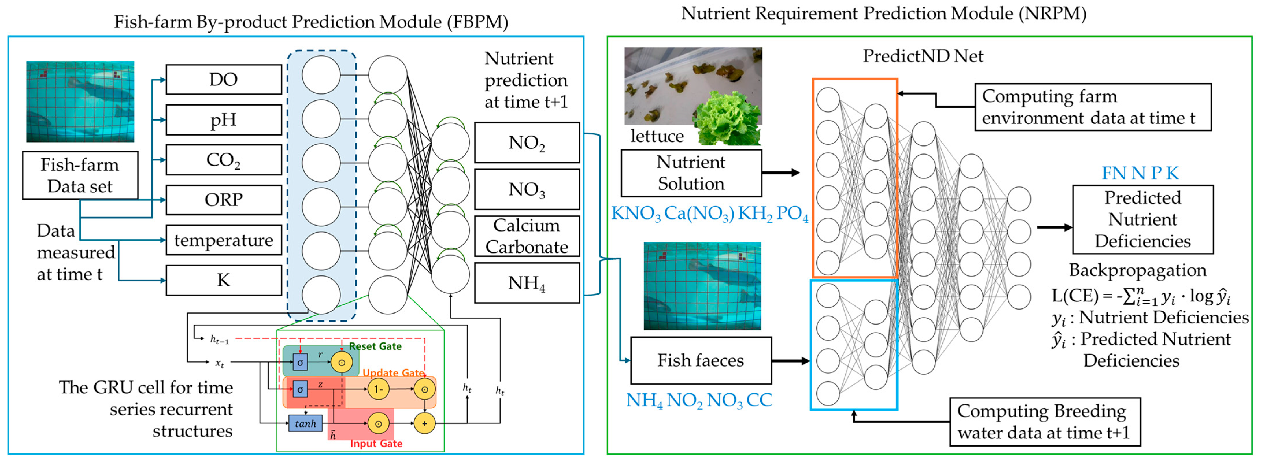
Figure 1 summarizes the data and control flow used in this work: aquaculture sensor streams and operation records are ingested by FBPM to forecast inflow chemistry at $t+1$ (NH₄⁺/TAN, NO₂⁻, NO₃⁻, alkalinity). In parallel, hydroponic sensor streams and crop records at time $t$ are ingested by NRPM. The NRPM output is the recommended N/P/K supplementation at time $t$, which is evaluated through a forward mixing/constraint check to report post-dose EC/pH feasibility metrics. Any image-based estimation shown in the schematic is not part of the proposed method or experiments in this study.

At each decision step $t$, the hydroponic loop is approximated as a well-mixed control volume. Let $V$ denote the effective solution volume in the hydroponic reservoir and $∆V$ the transferred aquaculture inflow volume over the decision interval. Let $c_t$ be the vector of relevant dissolved components in the hydroponic solution (including nitrogen species proxies and alkalinity) and let ${\widehat{c}}_{t+1}^{in}$ be FBPM’s one-step-ahead prediction for the inflow chemistry at $t+1$. The mixed inflow-updated state before supplementation is approximated by

$$c_{t+1}^{mix}={\displaystyle \frac{V{c}_t+∆V{\widehat{c}}_{t+1}^{in}}{V+∆V}},$$

(1)

NRPM outputs elemental supplementation recommendations $d_t={\left[d_t^N,d_t^P,d_t^K\right]}^{\mathrm{\top }}$ in mg·L⁻¹, and the post-dose state used for constraint checks is represented as $c_{t+1}^{post}=c_{t+1}^{mix}+d_t$. Post-dose EC and pH feasibility are evaluated consistently through the same forward mixing/constraint check used throughout the evaluation protocol. Plant uptake and other unmeasured dynamics are not parameterized as explicit process models in this study; instead, they are implicitly reflected in the supervisor signals (historical fertigation records) used to train NRPM.

2.2. Fish-Farm By-Product Prediction Module (FBPM)

The Fish-farm By-product Prediction Module (FBPM) proposed in this study analyzes the nutrient content of water transferred to the hydroponic environment using sensor data collected from aquaculture tanks. As shown in Figure 1, FBPM utilizes sensor data gathered from the tanks, along with fish growth metrics, as the input to predict the concentration of nutrients in the culture water that are essential for hydroponic cultivation.

2.2.1. Dataset of the FBPM

FBPM inputs are limited to time-series numeric data (sensor streams, growth logs, operation records); image-based estimation is excluded from this study. This study uses time-series logs from aquaculture tanks and greenhouse systems (sensor streams and management records). Water-quality and environment logs are aligned on a 5–10 min grid; daily fish growth metrics are joined by nearest timestamp. Short gaps (≤15 min) are linearly interpolated; longer gaps are excluded. Targets for FBPM are next-step ammonia, nitrite, nitrate, and alkalinity. Sensor gaps typically arise from routine calibration/maintenance, temporary connectivity loss, or sensor fouling. We interpolate only short gaps (≤15 min) to preserve the continuity of recurrent-model inputs and exclude longer gaps to avoid injecting artificial dynamics. In aquaculture and aquaponics, most dissolved inorganic nitrogen in the water originates from feed input and subsequent fish excretion and microbial nitrification. As fish grow, biomass and typical feeding rates increase, which generally increases nitrogenous waste production (TAN/ammonium), and downstream conversion to nitrite/nitrate; nitrification also affects alkalinity. Therefore, fish length is not used as a control/actuation variable and is not assumed to causally drive short-term water-chemistry changes; it is included only as a slowly varying contextual proxy for biomass/feeding-load trends that are not fully observable from instantaneous sensors. During the logging period, the provider operated a single fish species under a consistent feeding protocol; therefore, species-dependent differences are constant within our dataset and are not explicitly modeled.

The process by which FBPM constructs the training dataset is as follows:

First, because FBPM receives sensor data and fish growth data as time-series inputs, the two types of data must be merged into a single input dataset. To achieve this, sensor readings and fish growth records are aligned based on their timestamps to ensure that corresponding data points are matched chronologically.

$$BL{\left(z_k\right)}_{nom}={\displaystyle \frac{BL\left(z_k\right)-\mathrm{m}\mathrm{i}\mathrm{n}\left(BL\right(z_i\left)\right)}{\mathrm{m}\mathrm{a}\mathrm{x}\left(BL\left(z_i\right)\right)-\mathrm{m}\mathrm{i}\mathrm{n}\left(BL\right(z_i\left)\right)}},$$

(2)

Equation (2) describes the sampling method for the body length data. Here, $BL{\left(z_k\right)}_{nom}$ denotes the normalized value ranging between 0 and 1, $BL\left(x\right)$ is the current body length of fish $x$, and $z_i:1,\dots ,n$, where $n$ represents the total number of fish. In other words, the current fish’s body length is sampled within the range of 0 to 1 based on the body lengths of the fish present in the training data.

The input data for the neural network within FBPM consists of three main components: time information, tank environmental data, and fish growth data. These are described as follows:

• Time

Date (Year/Month/Day) and time (Hour:Minute)

2.

Tank Environment

Dissolved oxygen (DO), water temperature, pH, carbon dioxide (CO₂), flow rate, and light intensity

3.

Fish Growth Information

Average body length

In summary, FBPM uses eight input nodes. Since it is based on a GRU (Gated Recurrent Unit) architecture, the input dataset is structured as a time-series sequence. The model operates under a supervised learning paradigm and thus requires ground truth labels. Accordingly, the generated input data are paired with target values, consisting of the concentrations of ammonia, nitrite, nitrate, and alkalinity measured at the corresponding time. This results in a complete training dataset for supervised learning.

2.2.2. Structure of the Neural Network Inside the FBPM

The architecture of the Fish-farm By-product Prediction Module (FBPM) consists of four layers. The input layer receives the real-valued input dataset described in Section 2.2.1 and maps each feature to its corresponding input node. Before being propagated to the hidden layers, the input data is first passed through a Batch Normalization (BN) layer, which standardizes the input distribution.

Batch normalization mitigates the sensitivity to weight initialization and accelerates the training process. Equations (3) and (4) illustrate how the BN layer computes the mean and variance of the input data:

$${\mu }_{Batch}={\displaystyle \frac{1}{m}}\sum _{i=1}^{m}I{N}_i,$$

(3)

$${\sigma }_{\left(Batch\right)}^2={\displaystyle \frac{1}{m}}\sum _{i=1}^m{(I{N}_i-{\mu }_{Batch})}^2,$$

(4)

The Batch Normalization (BN) layer normalizes the input data using the standard deviation. In Equation (3), $I{N}_i$ represents the real-valued data stored at the current input node, $m$ is the batch size, and ${\mu }_{Batch}$ denotes the mean of $I{N}_i$. Equation (4) defines ${\sigma }_{\left(Batch\right)}^2$, which is the variance of the input data calculated based on ${\mu }_{Batch}$. Equation (5) shows how to compute the normalized data $x_i$ using the results from Equations (3) and (4).

$$x_i={\displaystyle \frac{I{N}_i-{\mu }_{Batch}}{\sqrt{{\sigma }_{\left(Batch\right)}^2+ϵ}}},$$

(5)

In Equation (5), $ϵ$ is a small constant used to prevent division by zero during the normalization process. Finally, the BN layer uses learnable parameters $\gamma$ and $\beta$, which are specific to the layer, to scale and shift the normalized input. Equation (6) describes how the input to the BN node is calculated.

$$B{N}_i=\gamma x_i+\beta ,$$

(6)

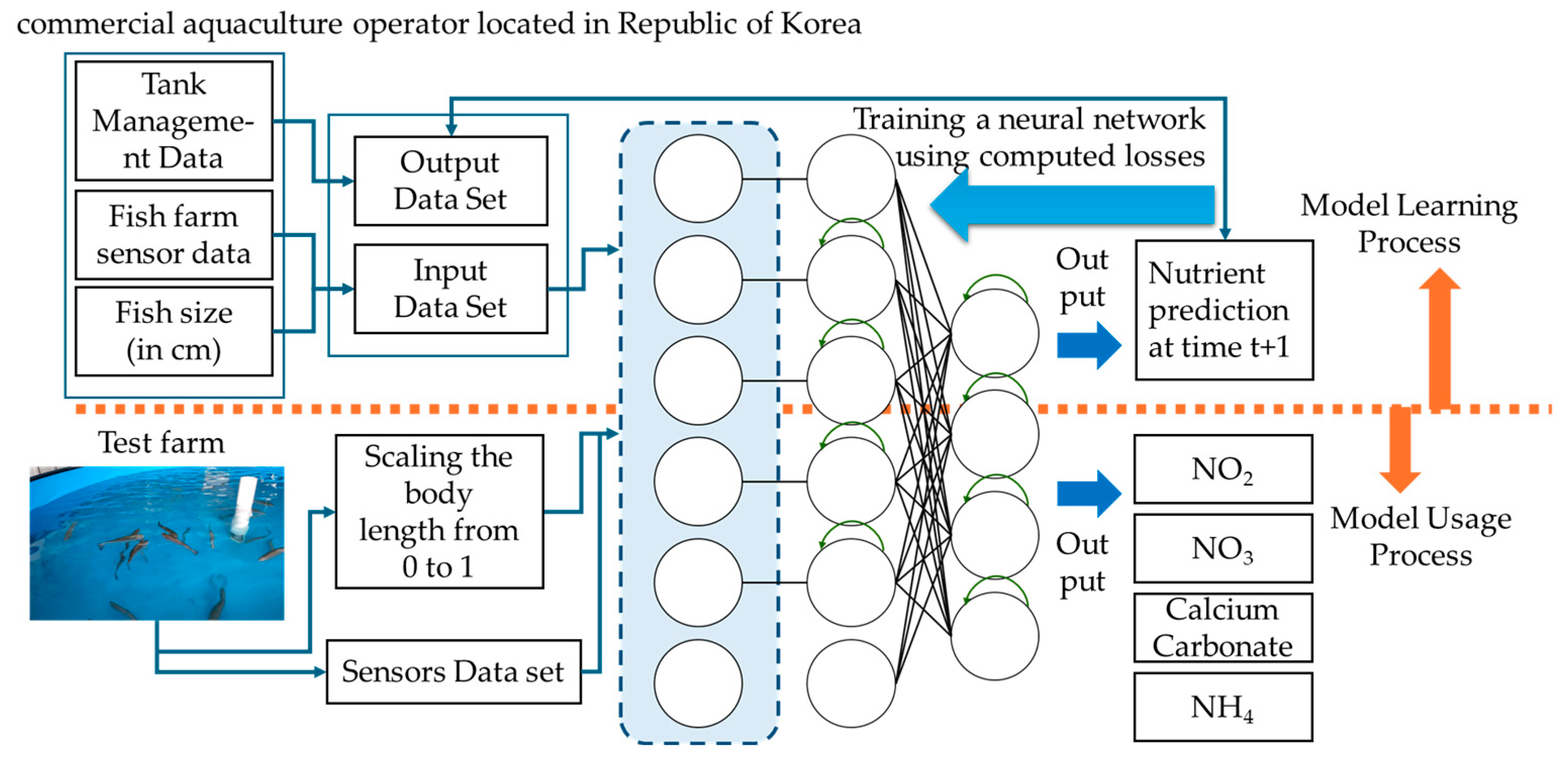
Figure 2 illustrates the FBPM pipeline. During training, the numeric input time series is normalized (Batch Normalization), encoded by GRU cells, and mapped to the target concentrations using supervised losses computed against measured labels in the logs. During inference, the same network produces one-step-ahead forecasts used as an exogenous driver for NRPM. The figure does not imply any imaging component in the present work. In this study, $\gamma$ represents the variance of $I{N}_i$, and $\beta$ denotes the mean of $I{N}_i$. Both $\gamma$ and $\beta$ are learned through backpropagation.

The batch size for training is set to 12. Data input to the Batch Normalization (BN) layer is then passed to the hidden layer, which consists of a two-layer GRU cell. Since using the ReLU (Rectified Linear Unit) activation function in GRUs can cause excessively large output values, this study adopts sigmoid and tanh functions instead. GRU-based deep learning models tend not to show significant performance gains with deeper hidden layers and are more prone to overfitting. Therefore, shallow architecture with two layers is employed.

2.3. Nutrient Requirement Prediction Module (NRPM)

In an aquaponics system, fish by-products alone are insufficient to fully meet the nutritional requirements of plants. Therefore, it is necessary to supplement the system with additional nutrient solutions to support proper plant growth. However, identifying which nutrients are present in the fish by-products and determining what nutrients are needed for plant growth cannot be easily accomplished through visual inspection or real-time manual monitoring.

To address this challenge, this study proposes the Nutrient Requirement Prediction Module (NRPM), which is designed to diagnose nutritional deficiencies in hydroponic environments. NRPM predicts the nutrients required in the next unit for hydroponic cultivation by following three main processes:

• Prediction of incoming fish-farm water nutrients:

The nutrient composition of the incoming aquaculture water, as predicted by the FBPM, is input into a single-layer neural network to allow NRPM to acquire information about the upcoming inflow conditions.

2.

Current hydroponic environment analysis:

Sensor data measured within the hydroponic environment at a specific time, along with the growth stage of the cultivated crop—categorized into three labeled stages—is used as input to another single-layer neural network. This allows the system to capture the current state of the hydroponic environment.

3.

Final nutrient requirement estimation:

Using the outputs from the above two stages, NRPM computes the required nutrient composition for the next unit time step to maintain optimal plant growth conditions.

2.3.1. Dataset of the NRPM

The Nutrient Requirement Prediction Module (NRPM) is trained to predict the nutrient requirements for plant growth based on two types of input data. The first input is the predicted water-quality data at time $t+1$, generated by the Fish-farm By-product Prediction Module (FBPM). The second input consists of environmental data collected at time $t$ from sensors within the hydroponic system, along with plant growth information.

The output from FBPM includes the concentrations of key nutrient components in the aquaculture water, namely ammonia (NH₄⁺), nitrite (NO₂⁻), nitrate (NO₃⁻), and alkalinity. This data is produced through a GRU-based time-series prediction module within FBPM and is fixed at the time point $t+1$. The predicted water-quality data is time-aligned to construct an input vector for NRPM based on temporal sequencing.

Meanwhile, the hydroponic environment data at time $t$ is derived from the “Intelligent Smart Farm Crop Growth Dataset” provided by a commercial aquaculture operator located in Yangyang-gun, Gangwon-do, Republic of Korea. In this study, environmental sensor data includes temperature (°C), humidity (%), CO₂ concentration (ppm), light intensity (lux), electrical conductivity (EC), and pH. Crop growth information comprises growth stage (early, middle, harvesting), fresh weight (g), plant height (cm), and leaf area (cm²). For transparency, the exact set of NRPM input/target variables and their sampling characteristics are enumerated in Appendix A (

Table A1. Inputs/targets used by FBPM and NRPM.

Module	Variable	Unit	Sampling	Role
FBPM	Dissolved oxygen (DO)	mg·L−1	5 min	Input
FBPM	Water temperature	°C	5 min	Input
FBPM	pH	—	5 min	Input
FBPM	Carbon dioxide (CO2)	ppm	5 min	Input
FBPM	Fish size/biomass proxy	—	daily	Input
FBPM	Flow rate	—	5 min	Input
FBPM	Light intensity	lux	5 min	Input
FBPM	Ammonium (NH4+)/TAN	mg·L−1	5 min	Target
FBPM	Nitrite (NO2−)	mg·L−1	5 min	Target
FBPM	Nitrate (NO3−)	mg·L−1	5 min	Target
FBPM	Alkalinity	mg·L−1 as CaCO3	5 min	Target
NRPM	EC	mS·cm−1	5 min	Input
NRPM	pH	—	5 min	Input
NRPM	Air temperature	°C	5 min	Input
NRPM	Relative humidity	%	5 min	Input
NRPM	CO2	ppm	5 min	Input
NRPM	Light intensity	lux	5 min	Input
NRPM	Growth stage	categorical	daily	Input
NRPM	Fresh weight/plant height/leaf area	g/cm/cm2	daily	Input
NRPM	FBPM forecast vector ($t+1$)	mg·L−1	aligned to 5 min	Input
NRPM	Dose labels (N/P/K)	mg·L−1	event-based, aligned to 5 min grid for learning	Target

).

The growth stage labels were qualitatively annotated by expert agronomists into three categories, and both the environmental and growth-related data were quantitatively normalized to fit the input format of the model. All input vectors were standardized using a unified time unit and structured in a time-series format to ensure alignment with the FBPM output for seamless integration.

For supervised learning, the target labels for NRPM consist of fertilization records (nitrogen, phosphorus, potassium, etc.) maintained by professional crop managers. These labels reflect the actual amount of nutrient supplementation required based on plant growth conditions. This data structure is essential for training an advanced model capable of automatically predicting necessary nutrient adjustments in response to dynamic changes in the plant growth environment.

2.3.2. The Structure of NRPM

NRPM estimates the elemental supplementation levels (N, P, K; mg·L⁻¹) needed for the next control action by jointly encoding the current hydroponic state and the predicted aquaculture inflow at $t+1$ provided by FBPM. The model is designed for online use: it consumes the most recent time window ending at time $t$ and a one-step-ahead inflow vector for $t+1$, then outputs non-negative supplements while respecting operational bounds on EC and pH. Let $w$ be the window length and 5 min the logging interval. The input consists of:

• Current-state window ${\mathbf{X}}_t\in {\mathbb{R}}^{w\times d}$. covering $[t-w+1,\dots ,t]$. Features (see Table A1) typically include:

EC, pH, solution temperature, greenhouse variables (air temp, RH, CO₂, light), growth indicators (daily mean weight/length), and recent operations (last supplementation amounts/events).

• Predicted inflow at next step ${\mathbf{q}}_{t+1}\in {\mathbb{R}}^4$ from FBPM: $[{\mathrm{NH}}_x-\mathrm{N},{\mathrm{NO}}_2-\mathrm{N},{\mathrm{NO}}_3-\mathrm{N},\mathrm{Alk}]$ of aquaculture water that will be fed into the hydroponic loop at $\mathrm{t}+1$.

(NRPM consumes ${\mathbf{q}}_{\mathrm{t}+1}$ as an exogenous driver; it does not re-predict water chemistry.)

All streams are re-sampled to a regular grid of 5 min; Each continuous feature is standardized (per site/season) and clipped at robust bounds to suppress sensor spikes. Recent supplementation features are encoded as magnitudes plus time-since-event. Categorical flags (e.g., water exchange) are one-hot. All targets and outputs are elemental: $\mathbf{y}=[\mathrm{N},\mathrm{P},\mathrm{K}]$ in mg·L⁻¹. If ionic quantities are referenced, conversions are:

$$\mathrm{N}=[{\mathrm{NO}}_3^{-}]\cdot {\displaystyle \frac{14}{62}}, \mathrm{P}=[{\mathrm{PO}}_4^{3-}]\cdot {\displaystyle \frac{31}{95}}, \mathrm{K}=[{\mathrm{K}}^{+}] (\mathrm{units} \mathrm{consistent} \mathrm{with} \mathrm{mg} {\mathrm{L}}^{-1}),$$

(7)

A current-state encoder $f_{\mathrm{curr}}$ (GRU/FC) maps ${\mathrm{X}}_t\mapsto {\mathrm{h}}_{\mathrm{curr}}$. An inflow encoder $f_{\mathrm{in}}$ (FC or shallow GRU over a 1-step stub) maps ${\mathrm{q}}_{t+1}\mapsto {\mathrm{h}}_{\mathrm{in}}$. The embeddings are concatenated and fused:

$$\mathrm{h}=\mathrm{Fuse}\left(\right[{\mathrm{h}}_{\mathrm{curr}};{\mathrm{h}}_{\mathrm{in}}\left]\right)\to \widehat{\mathrm{y}}=\mathrm{Softplus}\left(\mathrm{MLP}\right(\mathrm{h}\left)\right),$$

(8)

Soft plus enforces non-negativity. During training, a constraint-aware loss adds penalties when the post-dose EC/pH would exceed permissible bands. The NRPM prediction procedure consists of the following key stages:

• Future State Prediction: Using the predicted nutrient content of the aquaculture water at $t+1$, as provided by FBPM, the model forecasts the future state of the hydroponic system.
• Current State Analysis: Based on real-time sensor data, the model analyzes the current condition of the plants and learns the interactions between environmental factors and crop physiology.
• Nutrient Prediction: By integrating the predicted water-quality data from FBPM and the current environmental state, NRPM predicts the type and quantity of supplemental nutrients required. This integration enables precise estimation of nutrient deficiency or excess.

It is important to note that while FBPM predicts water nutrient content for time $t+1$, NRPM analyzes the hydroponic environment at time $t$. This design is intentional, as it allows the system to detect potential nutrient mismatches between the incoming aquaculture water and the current farm state, thereby requiring nutrient prediction for $t+1$ while using t as the reference for current environmental conditions. 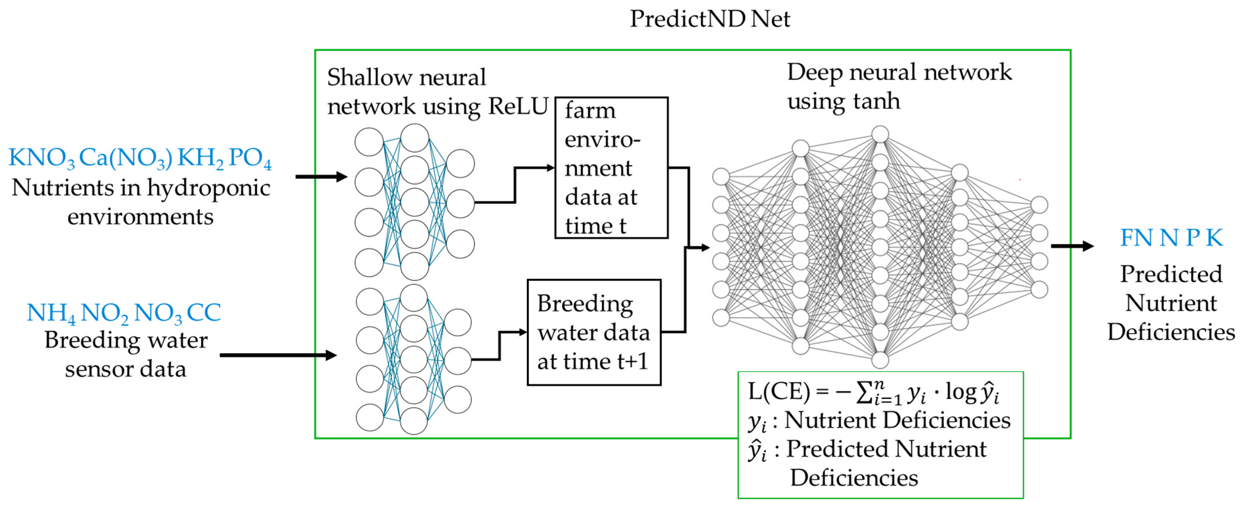Figure 3 illustrates process of NRPM. The NRPM consists of the following three stages:

• Stage 1—Water Nutrient Feature Extraction: The predicted nutrient concentrations from FBPM at time $t+1$ are processed through an input layer followed by a fully connected layer that performs nonlinear transformation, producing a compressed hidden vector. This stage enables the model to learn the impact of upcoming water nutrient composition on plant growth.
• Stage 2—Environmental Feature Extraction: The environmental data at time $t$, comprising sensor readings and plant growth stage labels, is passed through a separate fully connected layer. This step generates a feature vector that encapsulates both the current hydroponic conditions and the physiological characteristics of the crops.
• Stage 3—Feature Integration and Prediction: The two hidden vectors obtained from the previous stages are concatenated and passed through multiple dense layers. These layers use the ReLU activation function for nonlinear transformations, while the output layer uses Softplus to produce continuous non-negative N/P/K doses (mg·L⁻¹). The final output consists of the predicted supplementation levels for elemental N, P, and K (mg·L⁻¹), directly regressed by the output layer to align all outputs on an elemental basis.

The model is trained using the Mean Squared Error (MSE) as the loss function and optimized using the RMSProp algorithm to ensure both convergence speed and stability. Training is conducted with a batch size of 12 and 100 epochs, with dropout layers applied to select hidden layers to mitigate overfitting.

A key characteristic of NRPM is its ability to handle time-disjointed inputs in parallel and integrate them effectively. This architecture allows the model to resolve inconsistencies between the current crop environment and the predicted incoming aquaculture water, enabling optimized nutrient supplementation. Ultimately, NRPM contributes to improving the resource efficiency of hydroponic systems and enhancing the accuracy of plant growth prediction.

3. Results

We evaluate ASNRH under a fixed, protocol-first simulation to ensure the methods can be executed later without altering procedures. The evaluation addresses three questions. First, does fusing the greenhouse–crop state at time $t$ with the FBPM-predicted inflow at $t+1$ improve the regression of next-step supplementation (N/P/K, mg·L⁻¹) compared with strong baselines? Second, does encoding EC and pH as first-class constraints in the objective reduce safety violations more effectively than post hoc rule checks while maintaining accuracy? Third, how robust is the approach to typical field artifacts—namely missing observations and sensor noise?

The datasets used in this study were provided by a commercial aquaculture operator located in Yangyang-gun, Gangwon-do, Republic of Korea. The data were collected from the operator’s production system and shared under a data-use agreement; therefore, the company name and certain operational identifiers are anonymized. All time-series signals were aggregated to a uniform grid (5 min) for model training and evaluation.

The dataset comprises greenhouse environmental signals (temperature, relative humidity, ${\mathrm{C}\mathrm{O}}_2$, photosynthetic light, EC, pH) and crop growth indicators, together with aquaculture inflow chemistry required by FBPM (${\mathrm{N}\mathrm{H}}_4^{+}$, ${\mathrm{N}\mathrm{O}}_2^{-}$, ${\mathrm{N}\mathrm{O}}_3^{-}$, alkalinity). All continuous streams are re-sampled onto a 5 min grid and standardized per site and season to mitigate distributional shifts. NRPM consumes a sliding window of the current state $[t-W,t]$ and the FBPM forecast for $t+1$; unless otherwise noted, we set $W=4$ h and later examine horizons of 2 and 8 h. We set the default horizon to 4 h to match practical dosing/update intervals and mixing/response time in recirculating loops. To prevent temporal leakage, we use chronological splits of 60/20/20 for training/validation/test, and where available we also evaluate cross-season or cross-site generalization. Table 2 summarizes sources, grid, periods, and sample counts.

NRPM adopts a dual-branch encoder (current greenhouse–crop state; predicted inflow at $t+1$) followed by representation fusion and a Softplus output to enforce non-negative doses. The loss combines mean-squared error with penalties applied to post-dose EC and pH computed via a simple forward mixing model; an ${\mathcal{l}}_1$ smoothness term (mean absolute change between adjacent-step doses) on consecutive dose recommendations discourages unnecessary actuation volatility. FBPM is a lightweight GRU forecaster for inflow chemistry. Baselines include a persistence model (repeating the last dose) and a single-branch GRU that removes the inflow branch. Training is standardized across models with RMSProp, batch size 12, 100 epochs, and fixed random seeds; early-stopping is disabled to keep training schedules comparable.

Regression accuracy is reported as MAE, RMSE, and $R^2$ on the test split. Operation-oriented metrics include EC/pH violation rate (the fraction of test windows whose post-dose EC or pH falls outside agronomic bands defined earlier in the paper) and actuation smoothness, measured as the mean absolute change in recommended N/P/K between adjacent time steps. Robustness is quantified under MCAR missingness of 5–20% applied to sensor streams and additive Gaussian noise with standard deviation equal to half the empirical sensor SD. Unless specified otherwise, we report point estimates together with 95% confidence intervals (CIs) computed via a block bootstrap (moving-block) over contiguous test windows (block length L; B = 1000 resamples; 2.5th–97.5th percentiles).

Let ${\widehat{\mathrm{y}}}_t\in {\mathbb{R}}_{\ge 0}^3$ denote the recommended N/P/K at time $t$. We minimize:

$$\mathcal{L}=\underset{\mathrm{accuracy}}{\underbrace{\mathrm{MSE}(\widehat{\mathrm{y}},\mathrm{y})}}+{\lambda }_{\mathrm{EC}}\varphi ({\mathrm{EC}}_{\mathrm{post}})+{\lambda }_{\mathrm{pH}}\psi ({\mathrm{pH}}_{\mathrm{post}})+{\lambda }_{\mathsf{\Delta }}\parallel {\widehat{\mathrm{y}}}_t-{\widehat{\mathrm{y}}}_{t-1}{\parallel }_1,$$

(9)

We first train FBPM and materialize its $t+1$ forecasts for the entire timeline. NRPM is then trained on $[t-W,t]$ plus the stored $t+1$ forecasts. Ablations isolate the contribution of the inflow branch, constraint penalties, output non-negativity transform, and lightweight physics prior; window-length sensitivity is also analyzed. Robust experiments are conducted on the trained ASNRH model without re-tuning.

Table 3. Regression accuracy results of single-branch GRU and ASNRH. MAE/RMSE are reported as mean ± SD (bootstrap replicates, moving-block bootstrap over test windows, B = 1000).

Model	MAE-N	MAE-P	MAE-K	RMSE-N	RMSE-P	RMSE-K	${\mathit{R}}^2$-Avg	EC Viol. (%)	pH Viol. (%)	Volatility
Single-branch GRU	3.1 ± 0.4	2.2 ± 0.3	2.8± 0.5	4.6 ± 0.6	3.3 ± 0.4	4.1 ± 0.5	0.65	7.3	5.4	6.0
ASNRH	2.6 ± 0.3	1.8 ± 0.2	2.3 ± 0.2	3.8 ± 0.4	2.6 ± 0.3	3.4 ± 0.3	0.72	4.2	3.1	4.9

and

Table 4. Robustness under missingness/noise (ASNRH).

Condition	MAE-Avg	${\mathit{R}}^2$-Avg	EC Viol. (%)	pH Viol. (%)	Δ vs. Clean (MAE, R2, EC, pH)
Clean	2.23	0.72	4.2	3.1	—
MCAR 10%	2.61	0.66	5.8	4.1	+0.38, −0.06, +1.6, +1.0
Noise 0.5 SD	2.49	0.69	5.1	3.7	+0.26, −0.03, +0.9, +0.6

define ablation settings and organize the main/robustness results.

Where $\varphi ,\psi$ activate only when post-dose EC or pH exceed the allowed bands (bands specified in Table 1). The forward model uses standard mixing and electroneutrality approximations; precise constants (e.g., dose volume, recirculation fraction) are taken from the system configuration described in Section 2. The principal comparison across models is organized as Table 3, and the robustness outcomes as Table 4.

All experiments use the same optimizer (RMSProp), batch size (12), and epoch budget (100) with fixed seeds.

4. Discussion

This study reframes hydroponic nutrient dosing in aquaponics as an explicitly asynchronous decision: recommendations at time t must anticipate an inflow that materializes at $t+1$. By fusing the current hydroponic cultivation area–crop context with FBPM’s one-step-ahead inflow forecast, ASNRH reduces myopia relative to models that condition only relative to “now.” This information structure is particularly relevant for nitrogen-related dynamics, where inflow variability and delayed plant/solution responses co-exist.

Across evaluations, the benefit of explicitly modeling feasibility within learning is not limited to conventional regression accuracy. Treating EC and pH as first-class constraints inside the learning objective (rather than post hoc checks) consistently reduces the frequency of unsafe recommendations and discourages abrupt actuation changes. In practice, this shifts a portion of safety enforcement from downstream rule-based logic back into the learned mapping, which is useful for deployment settings where operators seek stable, bounded dosing schedules.

From a system perspective, decoupled aquaponics reduces direct water-quality conflicts between fish and plants, but it does not eliminate the operational coupling created by delayed inflow and recirculation. Even in decoupled layouts, the hydroponic controller still faces an anticipation problem: the same dose can be conservative or unsafe depending on how the next inflow moves the solution state. The proposed branch-and-fusion design addresses this coupling structurally by aligning “current demand” ($t$) with “imminent supply” ($t+1$) before producing the next-step recommendation.

Relative to model predictive control (MPC), which provides explicit constraint handling but typically requires a calibrated process model and controller design, ASNRH learns a direct mapping from sensed/logged state to dose while still internalizing feasibility through penalties and output constraints [21,22,23,24,25]. Relative to reinforcement learning (RL), which can optimize long-horizon objectives but often requires careful reward design and additional safety machinery (e.g., constrained learning and/or off-policy safety evaluation) before being trusted in real operations, ASNRH remains supervised and can be trained from historical operator logs while still expressing operational constraints in the objective [30,31,32].

Two caveats deserve attention. First, NRPM’s utility depends on the quality of FBPM’s inflow forecasts; miscalibration can propagate to systematic under- or over-dosing. This motivates careful training, monitoring, and periodic recalibration when drift is detected. Second, the weights on EC/pH penalties mediate a trade-off between conservatism and productivity: excessive weights may lead to chronic under-dosing, whereas insufficient weights may fail to suppress out-of-band states. The ablations and robustness experiments are therefore important not only as accuracy checks but also as guidance for selecting deployment-relevant operating points.

5. Conclusions

This study presented ASNRH, a two-module framework that couples FBPM’s $t+1$ inflow forecasts with the hydroponic cultivation area–crop state at time $t$ to directly regress non-negative next-step elemental N/P/K supplementation. We evaluated the framework under a protocol-first simulation with leakage-free chronological splits, reporting both standard regression metrics and operation-oriented criteria (post-dose EC/pH feasibility and actuation smoothness), and conducted ablations/robustness tests to isolate the contribution of the inflow branch and constraint-aware learning components. Overall, ASNRH provides a deployable decision-support approach for next-step nutrient supplementation that explicitly accounts for delayed inflow effects and EC/pH feasibility constraints in aquaponics. This design can facilitate sustainability-oriented operation by promoting resource-efficient supplementation from aquaculture byproducts and potentially reducing avoidable over-supplementation and subsequent corrective actions.

Our experiments are simulation-based and rely on simplified forward mixing assumptions for post-dose EC and pH checks; therefore, unmodeled hydraulic/micro-scale effects are not captured. FBPM forecasts are used as fixed inputs to NRPM, so forecast drift can propagate to dosing. Penalty weights in the constraint-aware objective are pre-specified rather than adaptively tuned; exploring adaptive weighting or multi-objective tuning is outside the scope of this study and is left for future work.