Article

NDVI Performance for Monitoring Agricultural Energy Inputs Using Landsat Imagery: A Study in the Ecuadorian Andes (2012–2023)

by
Pedro Zea
1,2,
Cristina Pascual
1,*,
Luis G. García-Montero
1 and
Hugo Cedillo
1,2
1
Centro para la Conservación de la Biodiversidad y el Desarrollo Sostenible (CBDS), E.T.S.I. Montes, Forestal y del Medio Natural, Universidad Politécnica de Madrid (UPM), 28040 Madrid, Spain
2
Grupo de Ecología Forestal Agroecosistemas y Silvopasturas en Sistemas Ganaderos, Facultad de Ciencias Agropecuarias, Universidad de Cuenca, Cuenca 010107, Ecuador
*
Author to whom correspondence should be addressed.
Sustainability 2025, 17(8), 3480; https://doi.org/10.3390/su17083480
Submission received: 27 January 2025 / Revised: 28 February 2025 / Accepted: 13 March 2025 / Published: 14 April 2025
(This article belongs to the Section Energy Sustainability)

Abstract

:
The NDVI is typically associated with medium-resolution images, e.g., Landsat imagery, and has often been linked to various agricultural parameters, except agricultural energy inputs. Thus, our objective was to analyze the performance of the NDVI associated with Landsat images to monitor both the evolution and impact of energy inputs on the spectral activity in some rural mountain crops. To do so, we studied energy inputs in three scenarios in the Ecuadorian Andes: high-mountain agroforestry systems (HAFSs), short-cycle production systems (SHCs), and low-mountain agroforestry systems (LAFSs). In 2022, information on energy inputs was collected for 415 systems (through field surveys). Using Google Earth Engine, we analyzed NDVI data associated with Landsat images between 2012 and 2023. Statistical analysis demonstrated significant positive correlations between energy inputs and the NDVI. As a novelty, this result means that energy inputs influence crops’ spectral activity. Furthermore, we demonstrated a historical enhancement of energy inputs across the inputs at the Landsat image scale. Therefore, further studies are needed to improve the resolution of this approach, for example, by integrating higher-resolution images to assess a more accurate NDVI response.

1. Introduction

1.1. Background

Food security and sustainable development require understanding of the land use in agricultural areas and its evolution in space and time [1,2,3]. They also require considering the ecological footprint as an indicator of crops’ impact on the environment [4]. The environmental footprint is currently used to assess energy supply and use in natural resources, land use, and waste production [5,6].
In recent times, various studies and land use plans have strengthened food security and sustainable development needs in the Andean region of Ecuador. This region stands out for its high biodiversity, but it also faces serious vulnerability in its rural population and several environmental and socioeconomic problems of international relevance [7].
For improving food security and sustainable development in agricultural scenarios, managing temporal crop information is crucial, as is data on cultivation phenology, because decision-makers can use it to make informed decisions on soil management, nutrient use, and water allocation by farmers [8,9,10]. One way to handle temporal information is using remote sensing. Landsat imagery is a suitable source for the long-term analysis of land cover change [3], with its 30 m spatial resolution, 8–16 day repeat cycle, and multispectral bands in images observed continuously for more than 40 years. As such, it provides an unparalleled opportunity to monitor crop dynamics, deforestation, and climate change mitigation worldwide [11,12,13].
Access to Landsat time series during crop development is crucial for this research. For this purpose, Google Earth Engine (GEE), a cloud computing platform, has transformed remote sensing data analysis by offering extensive pre-installed geospatial datasets and parallel processing capabilities. It provides global data on land use change, urbanization, human activity, environment, agriculture, water management, among other aspects, mainly obtained from sources such as Landsat, MODIS, Sentinel-2, and gridded meteorological data. This platform is instrumental in our study as it allows us to consider all images during the growing season, rather than being limited to a particular stage [14,15,16,17,18,19,20,21,22,23,24,25,26,27,28].

1.2. Problem Statement

In the Andean region of Ecuador, there is systematic difficulty in using Landsat imagery because of the intense cloudiness during the crop-productive months [29]. Google Earth Engine provides efficient algorithms for automatically detecting clouds and cloud shadows, which benefits various remote sensing activities and facilitates the generation of valuable Landsat time series collections for vegetation analysis [30]. As a result, responses in the red-visible and near-infrared spectra can be efficiently analyzed to calculate the Normalized Difference Vegetation Index (NDVI), which is widely used to assess vegetation density and health. This index is critical for monitoring the rapid variations in vegetation that occur at the beginning and end of plant growing and crop seasons [31,32], allowing farmers and land managers to plan essential agronomic activities, such as irrigation, fertilization, pest control, and others [33,34], especially in the context of precision agriculture.
However, predicting crop quality using the NDVI poses unique challenges due to the intrinsic noise and variability of NDVI data at the field level [35,36]. Thus, the use of data management and handling tools could bring us closer to a better understanding of the relationship between the NDVI and agriculture. Despite the availability of numerous Landsat image compositing algorithms, such as the NVDI, there are few comprehensive comparative studies analyzing their effectiveness [37]. Moreover, agronomically supported spectral detection limits have not been sufficiently explained [38]. The scientific literature highlights the importance of using the NDVI time series in conjunction with other data to describe the dynamics of crop production temporal patterns, soil surveys, agronomic management information, yield maps, topography, and soil electrical conductivity, as a requirement to identify stable crop patterns and to define management zones in intensive agriculture [39,40,41]. The existing studies on NVDI and crop management have already focused on plant nutrition and edaphic variables [42,43]. However, the possibility that the NVDI can be related to energy inputs in crop production has, to the best of our knowledge, not been studied before.
Historically, energy supply in crop production has been a central concern in global debates. On the other hand, the agricultural sector is not only an energy consumer but also the most crucial supplier of bioenergy [44,45]; thus, the assessment of crop energy management is essential to understanding agricultural efficiency, emphasizing both the productivity and sustainability of the sector [46]. A crucial aspect of farming and food production is the energy used per production unit. Several authors demonstrate the importance of determining energy inputs in agricultural productive systems [47] and highlight that excessive energy use generates environmental and health problems, underlining the need to study pollutant emissions and sustainable food production [48,49]. Therefore, understanding the current state of energy use efficiency in crop production at a precise spatial resolution, including in situ monitoring of crop energy inputs, is necessary to develop energy-saving strategies and optimize efficient crop production [50,51]. For this reason, food security studies often include recommendations on analyzing energy inputs and suggest that these could be based on historical data spanning several decades [52], such as those that Landsat image collections could provide.
Agriculture in the Andean region of Ecuador presents a strong altitudinal gradient, with climates that vary from warm climates with oceanic influence in low mountains to temperate climates typical of high equatorial mountains, which are home to a high diversity of crops that differ both in their plant species and in their agricultural intensification, energy inputs, and technology. These production systems vary between subsistence agriculture located in the highest areas versus low-mountain crops, with more intensive and somewhat more technologically advanced agriculture. This Andean subsistence agriculture is located on steeper slopes and in colder climates, characterized by small farms with little technology and lower energy inputs, but with a production of great importance for local food security, where short-cycle crops and/or agroforestry systems dominate. In contrast, low-mountain crops have greater economic importance at different scales (local, regional, and even national or international). They are located on gentler slopes and in warmer climates, where more intensive crops with higher energy inputs predominate [53,54]. Despite their geographical proximity, the population of both agrarian systems presents significant socioeconomic differences. In the highest land areas, there are more important problems of depopulation associated with emigration [55], which contrasts with the greater stability of the population in the lowest land areas, with better economic and employment conditions.

1.3. Research Objectives and Relevance

In this context, the main objective of this work was to verify whether the energy inputs of crops would significantly impact the normalized vegetation index (NDVI) as a tool to measure the efficiency and sustainability of Andean crops. To this end, we used a time series of Landsat images associated with smallholder subsistence farms and intensive farms in the Ecuadorian Andes region, which we systematically analyzed for changes in the NDVI over time (2012–2023). We used GEE to generate different types of Landsat images to assess spectral differences across a gradient of energy inputs, which allowed comparing three agricultural scenarios ranging from low-intensity to high-intensity agricultural use: (1) high-mountain agroforestry crops (mainly with fruit trees); (2) high-mountain short-cycle crops; and (3) low-mountain agroforestry crops (mainly with cocoa). We developed a secondary objective, based on a systematic experimental design in the field, to achieve this primary objective, allowing us to know the energy inputs in the three scenarios. Furthermore, to address the systematic cloudiness problem in the study area, a third objective was to extend the Landsat analysis to a significant period of years, allowing us to compare the performance of different types of images for better discrimination of a vegetation index.

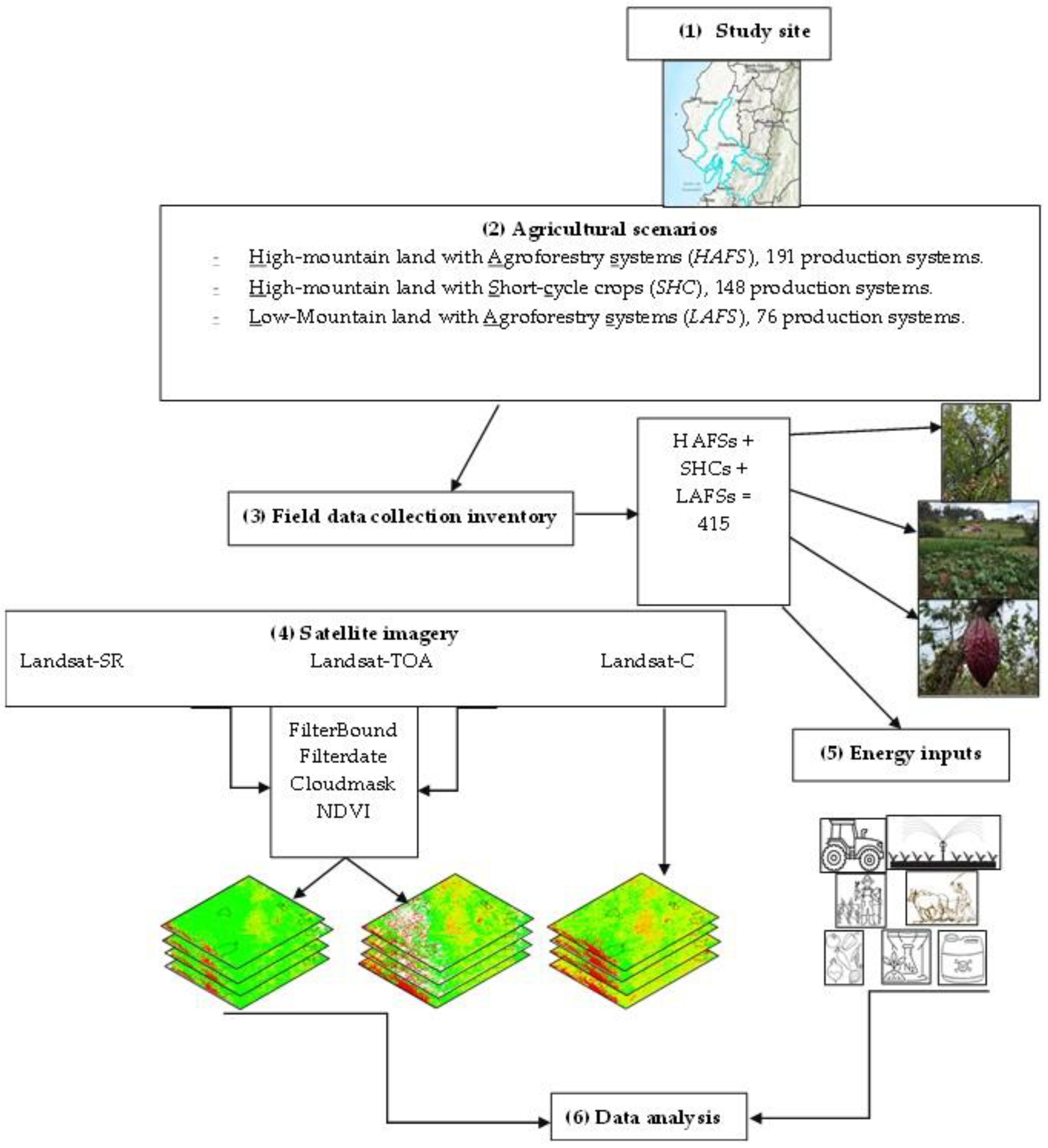
2. Materials and Methods

Figure 1 shows the workflow that summarizes the steps and the references to the methodology used in this work.

2.1. Study Site

2.1.1. Agricultural Scenarios

The research was carried out in the southern Andes region of Ecuador (Figure 2). In the high mountains of the Azuay province, we found the studied crop systems in the parishes of Bulán (2265–3125 m.a.s.l.), Principal (2445–2870 m.a.s.l.), and Cutchil (2505–2816 m.a.s.l.), where the average temperature was 11.1 °C and annual rainfall reached 964 mm. In the low mountains of the Cañar and Guayas provinces, the studied crop systems were in the parishes of La Troncal (90–110 m.a.s.l.) and Balao (0–10 m.a.s.l.), where the average temperature was 24.6 °C and annual rainfall reached 1274 mm. The climatic data were obtained from the WorldClim database [56]. We selected the studied scenarios because of their historical and current productive importance, according to thematic maps of land use and agricultural suitability [57], which allowed us to define their uses and agroecological qualities.
The studied parishes were divided into different scenarios according to their agronomic and geographical characteristics (Table 1 and Figure 3). The first scenario was High-mountain land with agroforestry systems (Scenario 1: HAFSs), which included deciduous and annual fruit and non-timber forest crops. The second scenario was another high-mountain land with short-cycle crops (Scenario 2: SHCs), which were predominantly associated with annual cultivations of corn, potatoes, legumes, and vegetables. Smallholder farmers have developed both scenarios on steep slopes. The third scenario was low-mountain land with agroforestry systems (Scenario 3: LAFSs), which, in the case of La Troncal parish, was characterized by cocoa crops, often associated with tropical fruit trees and managed by small producers, and in the case of Balao parish, was characterized by cocoa crops managed at the enterprise level. We found this third scenario on gentle slopes or flat areas.
Each of the scenarios had a significant number of farms, which, due to their integrity, average size, and diversity, were called ‘production systems’. In the described three scenarios, we randomly sampled and inventoried 415 production systems between November 2021 and February 2023. In the high-mountain scenarios (HAFSs and SHCs), we considered production system surfaces from 400 to 14,000 m2. While in the low-mountain scenarios (LAFSs), we considered production system surfaces from 600 to 135,000 m2. Each production system was systematically visited and georeferenced, and we collected its production and energy input data. The willingness of producers and local agricultural technicians was a key element in obtaining the field information.

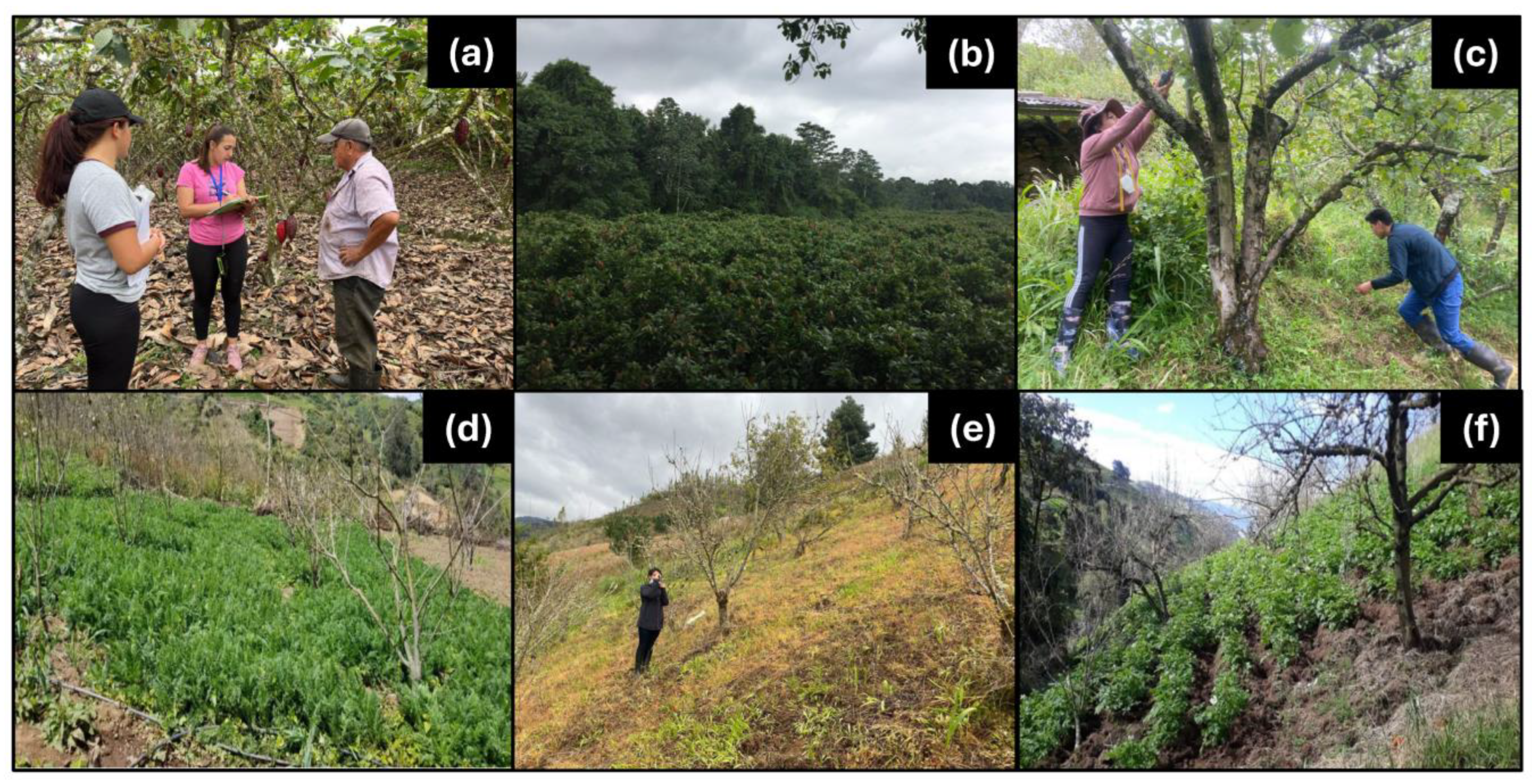
2.1.2. Field Data Collection/Inventory

To collect the information on each production system, we recorded the XY coordinates at the central point of the plot using a Spectra Precision Differential GPS. Farmers and technicians from the parishes, together with university students, provided us with support in field inventories (Figure 3).
In each production system, we collected interviews with the farmers, including production data and agricultural inputs, such as labor hours (regarding human and animal work), fuel consumption, fertilization (nitrogen, phosphorus, potassium, calcium, and magnesium), pesticides (herbicides, insecticides, and fungicides), plant material (seedlings and seeds), and amounts of irrigation water. We transformed all this information into homogeneous energy measures (GJ ha−1), following the procedures of Mobtaker et al. [58].

2.2. Satellite Imagery

We used a time series of Landsat images due to the availability of historical information (from 1980 to 2023), which facilitated historical monitoring of crops at medium resolution scale, with the potential to predict recent and future impacts of crops on rural populations and the environment [59]. We evaluated several methodologies and algorithms associated with Google Earth Engine (2024), focusing on optimizing the Normalized Difference Vegetation Index (NDVI) in the study area.
We focused on the productive period of crops in Ecuador (1 November to 30 April) to study the relationship between the NDVI and the energy input data in the production systems, which were analyzed between 2021 and 2023. We used Landsat composite maps because they had already been widely used to map land cover and land use change [60,61].
For the period studied, we used Landsat 8 and Landsat 9 images of Landsat surface reflectance (SR) (136 scenes), top of atmosphere (TOA) (487 scenes), and composite (C) (1 scene) (images were produced and available in GEE 2024, courtesy of the United States Geological Survey). The different image types are detailed in Table 2. We analyzed images in three-year ranges for a better quantitative analysis, following this pattern: (1) from 2012 to 2014, scenes were obtained from Landsat 5, Landsat 7, and Landsat 8 (however, for the period 5 May 2012 to 1 April 2013, only Landsat 7 images were considered due to data gaps in Landsat 5 and Landsat 8 during those months, considering the SLC-off after 31 May 2003); (2) for the years 2015–2017 and 2018–2020, scenes were obtained from Landsat 8; and (3) for the period 2021–2023, scenes were obtained from both Landsat 8 and Landsat 9 (to ensure a sufficient number of observations for the image composite). These three types of Landsat images were selected due to their specificity and accuracy of analysis in relation to the cloudiness problem [37], because, in the Andean Region, the agriculturally productive months have a cloudiness frequency of 68% [29]. We performed a preprocessing of these images to ensure that the NDVI is consistent across the different Landsat sensors (Figure 4).

2.3. Energy Inputs

Energy inputs are each of the inputs accounted for in their own units and transformed into homogeneous energy measures (GJ ha−1), and these energy equivalents were used to assess the energy inputs of production systems [49,62]. We classified inputs into the following categories: (1) work; (2) fertilizers; (3) pesticides; (4) vegetal issues; and (5) irrigation water. As in Kumar et al. [63], the energy summation of these was carried out according to Equation (1). Thus, the input data collected in the field inventory were converted into total energy inputs, with the energy equivalents displayed in Table 3, from multiple sources, especially from the tropics.
E T G J = Work + Fertilizers + Pesticides + Vegetal   issues + Irrigation   water
where, ET(GJ) is the total energy input, as the result of the sum of all inputs in Giga Joul: (1) work is the sum of the energy of human labor (hours)*, machine labor (hours)*, and animal labor (hours)*, plus the energy of the fuel used (kg)*; (2) fertilizers are the energy of the organic fertilizer (kg)* and chemical fertilizer (kg)*; (3) pesticides are the energy of herbicides (kg)* plus insecticides (kg)* plus fungicides (kg)*; (4) vegetal issues are the energy associated with the seeds (kg)* plus seedlings sown (kg)*; and finally, (5) irrigation water is the energy associated with the watering (m3)*. [* using the energy equivalents; see Table 3].

2.4. Image Processing

We obtained Landsat SR and TOA images from GEE. Then, we used specific algorithms that removed clouds, shadows, and bad pixels from the entire image collection [64]. No sensor calibration was applied, as the spectral properties from Landsat 4–9 were reasonably comparable, enabling dense spectral time series data [65,66].
Table 3. Energy equivalence of organic fertilizers, synthetic fertilizers, and other agrochemicals (herbicides, fungicides, and insecticides).
InputUnitMJ/UnitSource
Animal work (bovine)h5.05[67]
BiolL0.26[68]
Boronkg18.20[69]
Calciumkg8.80[70]
Chicken manurekg0.30[71]
Compostkg0.48[68]
Abonazakg13.38[72]
FuelL46.24[73]
Fungicideskg276[74]
Herbicideskg288[74]
Insecticideskg278[74]
Irrigation waterm31.02[75]
Work (labor)h1.96[73]
Limekg4.94[72]
Livestock workh0.58[76]
Machineryh62.70[77]
Magnesiumkg8.80[69]
Microelementskg120[78]
Nitrogenkg66.14[74]
Oilseedskg3.60[67]
Organic matterkg16.70[79]
Phosphoruskg12.44[74]
Potassiumkg11.15[74]
Seedlingsqty0.80[80]
Cereal and legume seedskg25[67]
Sulfurkg1.12[63]
Tuber seedskg14.70[67]
Zinckg8.40[70]
Landsat sensor (L5, L7, L8, and L9) band names were standardized to apply different functions and operations to all collection datasets. We calculated the NDVI for each image, one from each Landsat collection, using Equation (2).
N D V I = N I R R E D N I R + R E D
We used the maximum NDVI (Max_NDVI) across all three image types developed to analyze composite data [81] and to study the dynamic processes of terrestrial vegetation. This algorithm focused on selecting the observations with the highest NDVI of all observations within the study period (the composite of the images from the productive season), thus eliminating contamination by clouds and, potentially, snow or ice [37]. It was assumed that (i) the location of clouds was constantly changing and (ii) during a given period, cloud-free days existed at any location [82,83]. Some authors suggested using maximum NDVIs because these indexes were given more efficiency during the modeling, while NDVI points with low local values were assumed to be contaminated [84,85,86].
To evaluate the differences between the different types of NDVI images obtained, a quantitative statistical analysis of the data was carried out to highlight the differences between the surface reflectance, top of atmosphere, and composite images. All data used in this study are in a Supplementary File.

2.5. Data Analysis

In this study, a statistical analysis was conducted to assess the validity of the assumptions underlying the data. First, the multivariate Lilliefors test (also known as the Kolmogorov–Smirnov test) was applied to determine whether the data followed a normal distribution. In addition, Levene’s test was used to examine the homogeneity of variances between the groups of interest. When the assumptions of normality and homoscedasticity were not met, non-parametric statistical methods were used. Specifically, the Kruskal–Wallis test was used to compare the medians of three or more independent groups. Then, if significant differences were found, Dunn’s test, a post-hoc multiple comparisons test, was applied to identify between which groups such differences existed. Finally, to assess correlations between variables, Spearman’s non-parametric method was used, which does not require the assumption of normality to be met. This comprehensive approach allowed us to analyze the data rigorously and draw valid conclusions from the findings.
Statistical analysis was conducted using RStudio version ‘2024.12.0.467’ [87]. The data’s normality and the variance’s homoscedasticity were checked using the multivariate Lilliefors test (Kolmogorov–Smirnov) and Levene’s test, respectively, performed with the ‘MVN’ [88]. To evaluate the variance, we applied the Kruskal–Wallis test from the ‘Agricolae’ package [89], followed by Dunn’s test for multiple comparisons after finding a significant result from the Kruskal–Wallis test, which was performed with the ‘FSA’ package [90]. The graphs were created using the ‘ggplot2’ package [91]. The correlations were assessed using Spearman’s method from the ‘Inspect cor’ package [92]. The significance of the statistical analysis was identified at a p < 0.05 level.

3. Results

To assess the influence of energy inputs on the NDVI in the three scenarios, along a gradient of agricultural intensification and environmental conditions, a Spearman’s correlation between the MaxNDVI and energy inputs was performed for each production system, using the three Landsat collections. In addition, the evolution of NDVI values in the scenarios over time was studied by calculating the NDVI of the last decade.

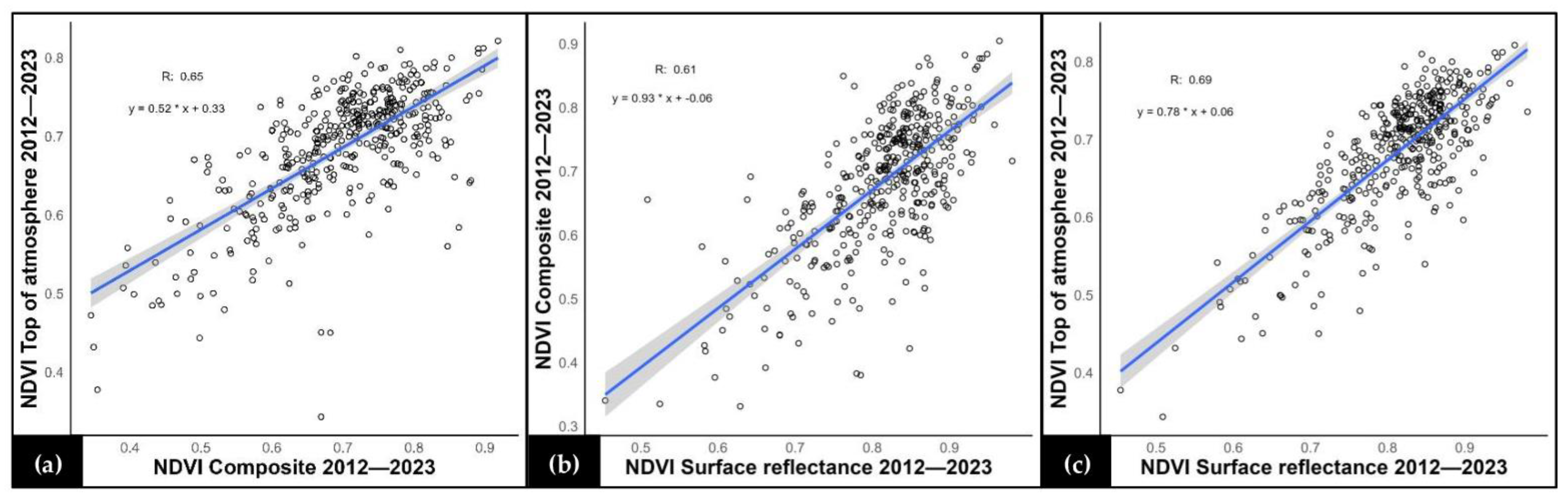
3.1. Relationship Between NDVI and Energy Input Data to Production Systems

The results of the farmers’ surveys, summarized in Table 4, indicated that fertilizers account for the largest share of energy inputs, at 55.46% of the total. Among the different studied farming systems, low-mountain agroforestry systems used the highest percentage of energy from fertilizers, at 76.3% of the total. In contrast, high-mountain short-cycle systems and high-mountain agroforestry systems showed a more equilibrated distribution of the different sources of energy inputs.
In total, we evaluated 488.97 ha of production systems located in the three described scenarios, in which 4066.56 GJ ha−1 of energy was invested in fertilizers (41.52 kg ha−1), of which 66.67% were synthetic fertilizers and 33.33% were organic fertilizers. Furthermore, we evaluated the synthetic fertilizers used, according to their composition and concentrations. We observed the following breakdown by nutrient importance: N = 61.6%; P = 11.5%; K = 10.3%; Ca = 8.19%; and Mg = 8.19% (Table 5).
Both energy and fertilizer inputs correlated very significantly with the NDVI data (obtained from the Landsat SR, TOA, and C images for each scenario) (Figure 5). For the SR images, statistical analysis indicated a positive correlation between the SR-NDVI and energy inputs, which was most decisive for the SHC scenarios (R = 0.28, R2 = 0.08, p = 0.0036). For the C images, statistical analysis indicated a positive correlation between the C-NDVI and energy inputs, which was most substantial for both LAFS (R = 0.26, R2 = 0.07, p = 0.03013) and SHC (R = 0.33, R2 = 0.11, p = 0.0039) scenarios. While for the TOA images, statistical analysis indicated that there was a positive correlation between the TOA-NDVI and energy inputs, which was most substantial for both LAFS (R = 0.36, R2 = 0.13, p = 0.0015) and SHC (R = 0.30, R2 = 0.09, p = 0.0014) scenarios. Figure 5 shows that trend lines showed a highly significant positive relationship between almost all NDVI values of the different images and energy inputs for all cases of the studied scenarios. Figure 5 also shows that the LAFS and SHC scenarios display a more compact distribution of the points. Finally, Figure 5 indicates that fertilizer was the most relevant variable among the energy inputs, showing highly significant correlations with the SHC-NVDI and LAFS-NVDI and displaying both productive systems with the highest amounts of fertilizer use.

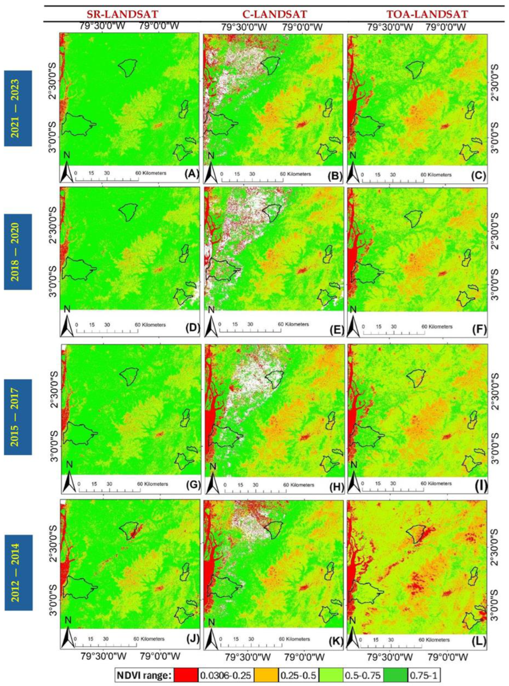
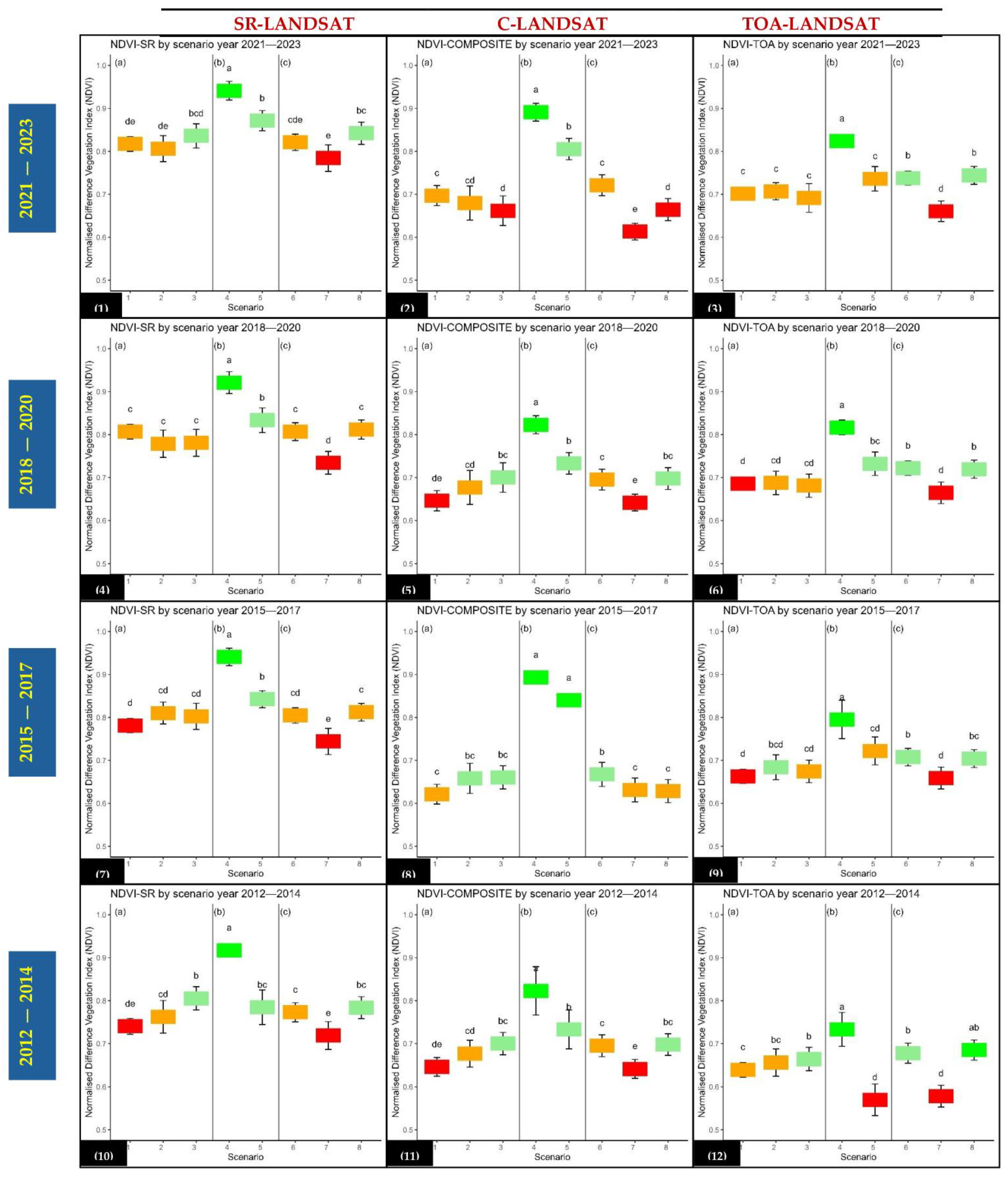
3.2. Changes in the NDVI over Time (2012–2023) in the Three Studied Agricultural Scenarios in the Andes of Ecuador

Figure 6 displays the Max_NDVI values in the studied area, showing the changes of this index over time in the SR, C, and TOA images, as well as the temporal evolution of the Max_NDVI from 2012 to 2023. The three types of Landsat images (SR, TOA, and C) have shown apparent differences in the visualization of their NDVI ranges and in the abundance of pixels masked by cloudiness (white pixels = no NDVI values), especially in C, which fortunately did not coincide mostly with the production systems. Thus, Figure 6 indicates that the SR images provided the best performance for analyzing the Max_NDVI values.
Figure 7 and Table 6 show the mean values of the Max_NDVI, according to image type (SR, TOA, and C), three-year period, and productive system types. There are significant differences in the Max_NDVI when comparing the different year periods and productive system types by scenario (p < 0.05) (Figure 7 and Table 6). The highest Max_NDVI values were found in the productive systems of the LAFS scenarios, which showed the higher energy inputs (cocoa productive systems characterized by medium to highly intensive agriculture), which contrasted with the productive systems of the SHC and HAFS scenarios, which showed the lower energy inputs (productive systems characterized by subsistence agriculture).
The image formats have similar ranges per year, but some differences exist. Regarding the Max_NDVI values, their patterns remained along the four periods of time for the three different types of images. Both the SR-NDVI and TOA-NDVI provided similar patterns. However, the SR-NDVI values were higher. Moreover, in the case of the TOA images, although we observed differences between the three production systems, the p-value was not significant (p > 0.05) (Figure 7 and Table 6).
On the other hand, when the Max_NDVI of the three Landsat formats were compared, significant correlations and regressions showed that, although the three formats of the images come from the same remote sensing source (Landsat), their different image processing processes provided a high and significant variability, shown in Figure 8, when comparing their Max_NDVI values, which values reached a correlation of 60% (r = 0.6; p < 0.05).

4. Discussion

In agriculture, spatial and temporal pattern analysis is a monitoring strategy used to assess changes in land use and vegetation [10,93]. In this sense, Farbo et al. [94] indicated that remote sensing and NDVI analysis in the growing and production seasons of crops are widely used to validate the results of agricultural actions in the field. These authors emphasized that the state of vegetation is a crucial factor in explaining crop yield, since the NDVI is a very effective indicator for assessing both plant health and productivity [31,32]. Therefore, NDVI analyses are fundamental for achieving proactive precision agriculture, where crop management could be significantly improved [94]. Different authors explained that high NDVI values in crops indicate stable and efficient agricultural production [39,40,41], even in mountain agricultural scenarios, where the efficiency of remote sensing may be limited [95].
When high-resolution images are used in the study of crop management, such as Sentinel images, Max_NDVI values are very sensitive and allow for the detection of all kinds of actions and patterns in crops, e.g., weed clearing and pruning, or tree canopy size in agroforestry systems, such as wine crops [27]. However, the results obtained in the present work have concluded that the use of medium-resolution images, such as Landsat images (30 m pixel), can also be very efficient for monitoring different crop management models in various agricultural scenarios, even in mountain areas. Thus, for example, in a study carried out by Anyimah et al. [96] on cocoa crops in Ghana, in which they used Sentinel TOA images, relatively high and constant NDVI values were obtained during the cocoa productive months, with maximum NDVI values of 0.58. In comparison, our results using Landsat-TOA images in cocoa crops in low-mountain scenarios (LAFSs) in the Ecuadorian Andes have also shown high Max_NDVI values (0.78), which have even been surpassed when using other image formats, such as Landsat-SR (0.92) and Landsat-C (0.86). In another example of Landsat-based mountain crop monitoring, such as the work of B. Yao et al. [97], values between 0.45 and 0.71 have been reported in the agricultural areas of the Yinshan Mountains in Mongolia. These values are also comparable to the Max_NDVI values observed in some of the mountain crops in the Ecuadorian Andes in the present work, such as the values obtained in the SHC scenario, where records of 0.80 for Landsat-SR, 0.67 for Landsat-C, and 0.78 for Landsat-TOA were obtained.
These results also allow us to underline the importance of optimizing the efficiency of Landsat images by using filters that improve their quality [30]. In this sense, Landsat-SR format images generated from Landsat-TOA images are the most used nowadays due to their high sharpness. However, the number of Landsat-SR images available is limited because they must meet specific quality criteria, such as the absence of clouds and the requirement for adequate calibration [98]. Therefore, in the present study in the Ecuadorian Andes, the availability of Landsat-SR images has been lower than that of Landsat-TOA images. Landsat surface reflectance improves the comparison between multiple images of the same region by accounting for atmospheric effects, such as aerosol scattering and thin clouds, which can help detect and characterize changes in the Earth’s surface. Surface reflectance is generated from level 1 input data that meet the solar zenith angle constraint of <76 degrees and include the ancillary input data necessary to generate a scientifically viable product (Landsat collection, courtesy of the USGS). However, Landsat-SR has been more efficient in analyzing the spatial patterns of the Max_NDVI and its statistical relationship with the energy inputs in crops. Qui et al. [37] have also compared the use of Landsat TOA and SR images to monitor NDVI values in different agricultural production systems in China, again confirming the greater efficiency of Landsat-SR images.
On the other hand, about Landsat-C images, we have carried out a bibliometric analysis from the Science Direct database, which has allowed us to conclude that, in research, Landsat-C images are being used less than Landsat-SR images but more than Landsat-TOA images. The results have indicated that these three types of images differ considerably from each other, since their spectral values only correlate in 60%. Therefore, depending on the specific research purposes, it would be necessary to either compare the suitability of each Landsat image or develop an ad hoc temporal image model.
In our study, where the main objective has been to analyze the agronomic impact of energy inputs on crops in different mountain scenarios, the Landsat-SR images have provided the highest values of Max_NDVI. These results have shown that increasing crop energy inputs over time can positively impact their Max_NDVI data. The results of our correlation and regression analyses have shown that, from a descriptive point of view, an intensification of agriculture based on an increase in crop energy inputs could generate a very significant footprint on the NDVI values of these crops. However, it was not possible to propose the opposite conclusion; that is, our results have not indicated that an improvement in the NDVI values observed in some crops over time did not necessarily mean that there would be an agricultural intensification in these crops that could be explained by an increase in energy inputs (due to the low levels of R2 values obtained in our statistical analysis).
According to the correlation analysis presented in Figure 5, two of the three scenarios evaluated, (LAFSs) and (SHCs), showed statistically significant correlations (p < 0.05). In contrast, (HAFSs) did not show statistical significance. The results suggested a moderate positive correlation (r = 0.36) between energy inputs and NDVI values. The p value = 0.0015 indicated that there was sufficient statistical evidence for the observed correlation to be attributable to chance. However, the R2 value = 0.13 indicated that only 13% of the variability in energy inputs could be explained by NDVI values, implying that many of the underlying causes were not captured by the current model.
Soil cover and its management are determining factors for the NDVI to show significant differences in the territory [44,98]. In the Kruskal–Wallis analysis of variance in the different types of NDVI contrasted with the production scenarios shown in Table 6, LAFSs, specifically, with Landsat surface reflectance, was significant (p > 0.05) in contrast to HAFSs and SHCs. This is because LAFSs have a homogeneous coverage of cocoa crops and a higher degree of vegetation cover than the other scenarios. In addition, NDVI values are usually associated with higher photo-synthetic activity, so a higher amount of fertilizer would be related to a higher amount of photosynthetic activity [99], and therefore, to higher NDVI values, which is the case in LAFSs and SHCs. In Figure 7, section “b”, in all the years evaluating the LAFSs were significant, in the case of SHCs and HAFSs they showed lower values, this could be due to the fact that these last scenarios were found in high areas and, generally, in lands with steep slopes, which could have influenced the quality of the NDVI, and it could even have happened due to the slope for the fertilization not being very efficient due to washing and erosion [100].
It is known that the use of fertilizers is correlated with the NDVI due to its direct impact on the health and activity of crop vegetation [101]. Recently, Manzur et al. [43] have indicated that soil nutrients, especially potassium (K) and phosphorus (P), are strongly related to NDVI values of crops. In the Ecuadorian Andes, the analysis of NDVI data over time and the results of the farmer surveys have indicated that there has been an agricultural intensification associated with an increase in energy inputs in some agricultural scenarios, which the fertilizers have mainly explained. These fertilizers have provided most of the energy inputs, representing 55.46%. In low-mountain agroforestry systems (cocoa crops), the effect of the fertilizers has been more pronounced in explaining their agricultural intensification, since 76.3% of their energy inputs come from their fertilization. However, the weight of each type of energy input (e.g., due to pesticides) in crops in different scenarios is very variable, since they depend on the specific agricultural dynamics of each territory [102,103,104].
In the studied area in the Ecuadorian Andes, on average, N, P, and K constituted 61.6%, 11.5%, and 10.3% of the fertilizer composition, respectively. Zhang et al. [105] have indicated that, under shade conditions, the application of nitrogen (138.0 kg ha−1) in agroforestry systems with deciduous tree crops can induce a significant increase in the photosynthetic area and the pigment content of the plants in these crops. Other authors, such as Benalcázar-Carranza et al. and Cai et al. [106,107], have confirmed that N is the most important nutrient among the fertilizers commonly used in different types of crops. Although N was the most important fertilizer used in the studied area in the Ecuadorian Andes, the amount per hectare was low (25.57 kg ha−1, on average). Furthermore, in the three studied scenarios, the use of organic fertilizers was 33.3% of the total inputs of this type of agricultural input. Gomiero et al. [108] have indicated the importance of intensifying the use of organic fertilizers because they improve soil quality and increase the sustainability of agricultural practices. In this regard, there is concern about the excessive dependence on synthetic fertilizers in agriculture globally. Ecuadorian farmers have managed fertilizers and other resources differently in the three studied scenarios. For instance, in the LAFS scenarios, the use of organic fertilizers decreased to 23.7% of the total inputs because in this low-mountain scenario, the cocoa crops have a productive design more oriented towards intensive agriculture [57]. These patterns could be explained by the fact that 81% of the studied Ecuadorian production systems in the present work have been managed by small producers, with whom training should be improved to avoid underutilization or inadequate use of fertilizers.

5. Conclusions

In summary, the results of the present study have validated the usefulness of using the NDVI associated with Landsat images (medium resolution) to monitor the efficiency of energy inputs in different mountain agricultural production systems in the Ecuadorian Andes. This result has been due to (i) the NDVI being a good spectral index to evaluate the health and productivity of crop vegetation and (ii) because Landsat-SR images are more efficient in the analysis of spatial patterns and in obtaining higher NDVI values than the Landsat-TOA images. Therefore, these images, when atmospherically corrected, offer more transparent and more precise data for studies of crop vegetation. Therefore, they may be an enjoyable alternative to higher resolution images, but with less availability of images in recent decades. As a consequence of this type of monitoring, our results have shown a low positive (13%, at most) but highly significant correlation between the Max-NDVI and energy inputs in crop production systems, especially concerning energy associated with fertilizers. The statistical significance (p = 0.0015) of this correlation is due to the fact that, despite being a weak relationship, it is highly reliable, with a 95% assumption, and is not due to chance. This indicates that, even with a modest correlation, there is a real association between the NDVI and energy inputs. Concerning the mountain agricultural scenarios compared across the study area, low-mountain agroforestry systems (LAFSs), with a more intensive agricultural model, are more dependent on energy inputs (mainly associated with fertilizers) compared to high-mountain agroforestry systems (HAFSs) and short-cycle crops (SHCs), with less intensive, more sustainable agricultural models, and with high importance for local food security. Thus, using the NDVI associated with medium-resolution images (Landsat; mainly SR format) is confirmed as a potential indicator for developing precision agriculture, even in mountain agricultural scenarios. However, further studies are needed to improve the resolution of this approach, for example, by integrating higher-resolution images to assess a more accurate NDVI response. For example, in modern studies (since 2017), Sentinel-SR imagery could be used as it is known to provide suitable data for assessing the status and change in vegetation, soil, and water cover, which could allow using the NVDI for monitoring crops, health, and energy efficiency, adjusting management practices and favoring a significant improvement in agricultural productivity and sustainability, which is especially important in vulnerable rural areas. These findings will serve as a basis for future research and the development of better management strategies in agriculture in the Andes of Ecuador and other comparable areas.

Supplementary Materials

The supporting database of inputs and NDVI values can be downloaded at: https://www.mdpi.com/article/10.3390/su17083480/s1.

Author Contributions

Conceptualization, P.Z., C.P. and L.G.G.-M.; methodology, P.Z., C.P. and L.G.G.-M.; software, P.Z. and C.P.; validation, L.G.G.-M. and H.C.; formal analysis, P.Z.; investigation, P.Z., C.P., L.G.G.-M. and H.C.; resources, P.Z.; data curation, P.Z.; writing—preparation of original draft, P.Z., C.P., L.G.G.-M. and H.C.; writing—review and editing, P.Z., C.P., L.G.G.-M. and H.C.; visualization, C.P.; supervision, L.G.G.-M. All authors have read and agreed to the published version of the manuscript.

Funding

This research received no external funding.

Institutional Review Board Statement

Not applicable.

Informed Consent Statement

Not applicable.

Data Availability Statement

The original contributions presented in this study are included in the article. Further inquiries can be directed to the corresponding author.

Acknowledgments

The authors would like to thank the University of Cuenca-Ecuador and the Polytechnic University of Madrid (Centro para la Conservación de la Biodiversidad y el Desarrollo Sostenible (CBDS) and E.T.S.I. Montes, Forestal y del Medio Natural), as well as the 415 Ecuadorian farmers, 15 agricultural technicians, and 10 undergraduate students of the Agronomy program at the University of Cuenca who contributed to the collection of information.

Conflicts of Interest

The authors declare no conflicts of interest.

Abbreviations

The following abbreviations are used in this manuscript:
NDVINormalized difference vegetation index
HAFSHigh-mountain agroforestry system
SHCShort-cycle production system
LAFSLow-mountain agroforestry system
GEEGoogle Earth Engine
GJGiga Joule
haHectare
SRSurface reflectance
TOATop of atmosphere
CComposite
SLC-offSLC-off defect of a Landsat 7 image collected after 31 May 2003
hHour
LLiter
kgKilogram
m3Cubic meter
USGSUnited States Geological Survey

References

  1. See, L.; Fritz, S.; You, L.; Ramankutty, N.; Herrero, M.; Justice, C.; Becker-Reshef, I.; Thornton, P.; Erb, K.; Gong, P.; et al. Improved Global Cropland Data as an Essential Ingredient for Food Security. Glob. Food Secur. 2015, 4, 37–45. [Google Scholar] [CrossRef]
  2. Pérez-Hoyos, A.; Rembold, F.; Kerdiles, H.; Gallego, J. Comparison of Global Land Cover Datasets for Cropland Monitoring. Remote Sens. 2017, 9, 1118. [Google Scholar] [CrossRef]
  3. Wijesingha, J.; Dzene, I.; Wachendorf, M. Evaluating the Spatial–Temporal Transferability of Models for Agricultural Land Cover Mapping Using Landsat Archive. ISPRS J. Photogramm. Remote Sens. 2024, 213, 72–86. [Google Scholar] [CrossRef]
  4. Stips, A.; Macias, D.; Coughlan, C.; Garcia-Gorriz, E.; Liang, X.S. On the Causal Structure between CO2 and Global Temperature. Sci. Rep. 2016, 6, 21691. [Google Scholar] [CrossRef] [PubMed]
  5. Bigerna, S.; Bollino, C.A.; Polinori, P. Convergence of Ecological Footprint and Sustainable Policy Options. J. Policy Model 2022, 44, 564–577. [Google Scholar] [CrossRef]
  6. John, M.A.; Ugwuoke, W.O.; Okwanya, I. Climate Change and Food Security Causality in ECOWAS Region: Do Countries Interdependence Matter? Food Humanit. 2024, 3, 100393. [Google Scholar] [CrossRef]
  7. Ayaviri-Nina, D.; Quispe-Fernández, G.; Romero-Flores, M.; Fierro-López, P. Avances y Progresos de Las Políticas y Estrategias de Seguridad Alimentaria En Ecuador. Rev. Investig. Altoandin. 2016, 18, 213–222. [Google Scholar] [CrossRef]
  8. Chen, J.; Jönsson, P.; Tamura, M.; Gu, Z.; Matsushita, B.; Eklundh, L. A Simple Method for Reconstructing a High-Quality NDVI Time-Series Data Set Based on the Savitzky–Golay Filter. Remote Sens. Environ. 2004, 91, 332–344. [Google Scholar] [CrossRef]
  9. Imeson, A.C.; Prinsen, H.A.M. Vegetation Patterns as Biological Indicators for Identifying Runoff and Sediment Source and Sink Areas for Semi-Arid Landscapes in Spain. Agric. Ecosyst. Environ. 2004, 104, 333–342. [Google Scholar] [CrossRef]
  10. Liepa, A.; Thiel, M.; Taubenböck, H.; Steffan-Dewenter, I.; Abu, I.-O.; Singh Dhillon, M.; Otte, I.; Otim, M.H.; Lutaakome, M.; Meinhof, D.; et al. Harmonized NDVI Time-Series from Landsat and Sentinel-2 Reveal Phenological Patterns of Diverse, Small-Scale Cropping Systems in East Africa. Remote Sens. Appl. Soc. Environ. 2024, 35, 101230. [Google Scholar] [CrossRef]
  11. Wulder, M.A.; Loveland, T.R.; Roy, D.P.; Crawford, C.J.; Masek, J.G.; Woodcock, C.E.; Allen, R.G.; Anderson, M.C.; Belward, A.S.; Cohen, W.B.; et al. Current Status of Landsat Program, Science, and Applications. Remote Sens. Environ. 2019, 225, 127–147. [Google Scholar] [CrossRef]
  12. Jiang, N.; Li, P.; Feng, Z. Remote Sensing of Swidden Agriculture in the Tropics: A Review. Int. J. Appl. Earth Obs. Geoinf. 2022, 112, 102876. [Google Scholar] [CrossRef]
  13. Zhao, H.; Zhou, Y.; Zhang, G.; Chen, X.; Chang, Y.; Luo, Y.; Jin, Y.; Pan, Z.; An, P. Mapping the Dynamics of Intensive Forage Acreage during 2008–2022 in Google Earth Engine Using Time Series Landsat Images and a Phenology-Based Algorithm. Comput. Electron. Agric. 2024, 221, 108983. [Google Scholar] [CrossRef]
  14. Hansen, M.C.; Potapov, P.V.; Moore, R.; Hancher, M.; Turubanova, S.A.; Tyukavina, A.; Thau, D.; Stehman, S.V.; Goetz, S.J.; Loveland, T.R.; et al. High-Resolution Global Maps of 21st-Century Forest Cover Change. Science 2013, 342, 850–853. [Google Scholar] [CrossRef]
  15. Miettinen, J.; Shi, C.; Liew, S.C. Land Cover Distribution in the Peatlands of Peninsular Malaysia, Sumatra and Borneo in 2015 with Changes since 1990. Glob. Ecol. Conserv. 2016, 6, 67–78. [Google Scholar] [CrossRef]
  16. Padarian, J.; Minasny, B.; McBratney, A.B. Chile and the Chilean Soil Grid: A Contribution to GlobalSoilMap. Geoderma Reg. 2017, 9, 17–28. [Google Scholar] [CrossRef]
  17. Hird, J.; DeLancey, E.; McDermid, G.; Kariyeva, J. Google Earth Engine, Open-Access Satellite Data, and Machine Learning in Support of Large-Area Probabilistic Wetland Mapping. Remote Sens. 2017, 9, 1315. [Google Scholar] [CrossRef]
  18. Asner, G.P.; Brodrick, P.G.; Philipson, C.; Vaughn, N.R.; Martin, R.E.; Knapp, D.E.; Heckler, J.; Evans, L.J.; Jucker, T.; Goossens, B.; et al. Mapped Aboveground Carbon Stocks to Advance Forest Conservation and Recovery in Malaysian Borneo. Biol. Conserv. 2018, 217, 289–310. [Google Scholar] [CrossRef]
  19. Bunting, E.L.; Munson, S.M.; Bradford, J.B. Assessing Plant Production Responses to Climate across Water-Limited Regions Using Google Earth Engine. Remote Sens. Environ. 2019, 233, 111379. [Google Scholar] [CrossRef]
  20. Ge, Y.; Hu, S.; Ren, Z.; Jia, Y.; Wang, J.; Liu, M.; Zhang, D.; Zhao, W.; Luo, Y.; Fu, Y.; et al. Mapping Annual Land Use Changes in China’s Poverty-Stricken Areas from 2013 to 2018. Remote Sens. Environ. 2019, 232, 111285. [Google Scholar] [CrossRef]
  21. Wong, B.A.; Thomas, C.; Halpin, P. Automating Offshore Infrastructure Extractions Using Synthetic Aperture Radar & Google Earth Engine. Remote Sens. Environ. 2019, 233, 111412. [Google Scholar] [CrossRef]
  22. Gong, P.; Li, X.; Wang, J.; Bai, Y.; Chen, B.; Hu, T.; Liu, X.; Xu, B.; Yang, J.; Zhang, W.; et al. Annual Maps of Global Artificial Impervious Area (GAIA) between 1985 and 2018. Remote Sens. Environ. 2020, 236, 111510. [Google Scholar] [CrossRef]
  23. DeVries, B.; Huang, C.; Armston, J.; Huang, W.; Jones, J.W.; Lang, M.W. Rapid and Robust Monitoring of Flood Events Using Sentinel-1 and Landsat Data on the Google Earth Engine. Remote Sens. Environ. 2020, 240, 111664. [Google Scholar] [CrossRef]
  24. Bey, A.; Jetimane, J.; Lisboa, S.N.; Ribeiro, N.; Sitoe, A.; Meyfroidt, P. Mapping Smallholder and Large-Scale Cropland Dynamics with a Flexible Classification System and Pixel-Based Composites in an Emerging Frontier of Mozambique. Remote Sens. Environ. 2020, 239, 111611. [Google Scholar] [CrossRef]
  25. Tian, J.; Wang, L.; Yin, D.; Li, X.; Diao, C.; Gong, H.; Shi, C.; Menenti, M.; Ge, Y.; Nie, S.; et al. Development of Spectral-Phenological Features for Deep Learning to Understand Spartina Alterniflora Invasion. Remote Sens. Environ. 2020, 242, 111745. [Google Scholar] [CrossRef]
  26. Gorelick, N.; Hancher, M.; Dixon, M.; Ilyushchenko, S.; Thau, D.; Moore, R. Google Earth Engine: Planetary-Scale Geospatial Analysis for Everyone. Remote Sens. Environ. 2017, 202, 18–27. [Google Scholar] [CrossRef]
  27. Devaux, N.; Crestey, T.; Leroux, C.; Tisseyre, B. Potential of Sentinel-2 Satellite Images to Monitor Vine Fields Grown at a Territorial Scale. OENO One 2019, 53, 52–59. [Google Scholar] [CrossRef]
  28. Wang, L.; Diao, C.; Xian, G.; Yin, D.; Lu, Y.; Zou, S.; Erickson, T.A. A Summary of the Special Issue on Remote Sensing of Land Change Science with Google Earth Engine. Remote Sens. Environ. 2020, 248, 112002. [Google Scholar] [CrossRef]
  29. Prudente, V.H.R.; Martins, V.S.; Vieira, D.C.; Silva, N.R.D.F.E.; Adami, M.; Sanches, I.D. Limitations of Cloud Cover for Optical Remote Sensing of Agricultural Areas across South America. Remote Sens. Appl. Soc. Environ. 2020, 20, 100414. [Google Scholar] [CrossRef]
  30. Zhu, Z.; Woodcock, C.E. Object-Based Cloud and Cloud Shadow Detection in Landsat Imagery. Remote Sens. Environ. 2012, 118, 83–94. [Google Scholar] [CrossRef]
  31. Pettorelli, N.; Vik, J.O.; Mysterud, A.; Gaillard, J.-M.; Tucker, C.J.; Stenseth, N.C. Using the Satellite-Derived NDVI to Assess Ecological Responses to Environmental Change. Trends Ecol. Evol. 2005, 20, 503–510. [Google Scholar] [CrossRef] [PubMed]
  32. Zhang, Y.; Gao, J.; Liu, L.; Wang, Z.; Ding, M.; Yang, X. NDVI-Based Vegetation Changes and Their Responses to Climate Change from 1982 to 2011: A Case Study in the Koshi River Basin in the Middle Himalayas. Glob. Planet. Change 2013, 108, 139–148. [Google Scholar] [CrossRef]
  33. Radočaj, D.; Šiljeg, A.; Marinović, R.; Jurišić, M. State of Major Vegetation Indices in Precision Agriculture Studies Indexed in Web of Science: A Review. Agriculture 2023, 13, 707. [Google Scholar] [CrossRef]
  34. Blaes, X.; Chomé, G.; Lambert, M.-J.; Traoré, P.; Schut, A.; Defourny, P. Quantifying Fertilizer Application Response Variability with VHR Satellite NDVI Time Series in a Rainfed Smallholder Cropping System of Mali. Remote Sens. 2016, 8, 531. [Google Scholar] [CrossRef]
  35. Cavalli, S.; Penzotti, G.; Amoretti, M.; Caselli, S. A Machine Learning Approach for NDVI Forecasting Based on Sentinel-2 Data. In Proceedings of the 16th International Conference on Software Technologies, Virtual Event, 6–8 July 2021; pp. 473–480. Available online: https://www.scitepress.org/PublishedPapers/2021/105445/105445.pdf (accessed on 12 September 2024).
  36. Ahmad, R.; Yang, B.; Ettlin, G.; Berger, A.; Rodríguez-Bocca, P. A Machine-learning Based ConvLSTM Architecture for NDVI Forecasting. Int. Trans. Oper. Res. 2023, 30, 2025–2048. [Google Scholar] [CrossRef]
  37. Qiu, S.; Zhu, Z.; Olofsson, P.; Woodcock, C.E.; Jin, S. Evaluation of Landsat Image Compositing Algorithms. Remote Sens. Environ. 2023, 285, 113375. [Google Scholar] [CrossRef]
  38. Heinemann, P.; Haug, S.; Schmidhalter, U. Evaluating and Defining Agronomically Relevant Detection Limits for Spectral Reflectance-Based Assessment of N Uptake in Wheat. Eur. J. Agron. 2022, 140, 126609. [Google Scholar] [CrossRef]
  39. Vélez, S.; Rançon, F.; Barajas, E.; Brunel, G.; Rubio, J.A.; Tisseyre, B. Potential of Functional Analysis Applied to Sentinel-2 Time-Series to Assess Relevant Agronomic Parameters at the within-Field Level in Viticulture. Comput. Electron. Agric. 2022, 194, 106726. [Google Scholar] [CrossRef]
  40. Ouazaa, S.; Jaramillo-Barrios, C.I.; Chaali, N.; Amaya, Y.M.Q.; Carvajal, J.E.C.; Ramos, O.M. Towards Site Specific Management Zones Delineation in Rotational Cropping System: Application of Multivariate Spatial Clustering Model Based on Soil Properties. Geoderma Reg. 2022, 30, e00564. [Google Scholar] [CrossRef]
  41. Sandonís-Pozo, L.; Oger, B.; Tisseyre, B.; Llorens, J.; Escolà, A.; Pascual, M.; Martínez-Casasnovas, J.A. Leafiness-LiDAR Index and NDVI for Identification of Temporal Patterns in Super-Intensive Almond Orchards as Response to Different Management Strategies. Eur. J. Agron. 2024, 159, 127278. [Google Scholar] [CrossRef]
  42. Gopp, N.V.; Savenkov, O.A. Relationships between the NDVI, Yield of Spring Wheat, and Properties of the Plow Horizon of Eluviated Clay-Illuvial Chernozems and Dark Gray Soils. Eurasian Soil Sci. 2019, 52, 339–347. [Google Scholar] [CrossRef]
  43. Mazur, P.; Gozdowski, D.; Wójcik-Gront, E. Soil Electrical Conductivity and Satellite-Derived Vegetation Indices for Evaluation of Phosphorus, Potassium and Magnesium Content, pH, and Delineation of Within-Field Management Zones. Agriculture 2022, 12, 883. [Google Scholar] [CrossRef]
  44. Zanaganeh, M.; Mousavi, S.J.; Etemad Shahidi, A.F. A Hybrid Genetic Algorithm–Adaptive Network-Based Fuzzy Inference System in Prediction of Wave Parameters. Eng. Appl. Artif. Intell. 2009, 22, 1194–1202. [Google Scholar] [CrossRef]
  45. Hosseinzadeh-Bandbafha, H.; Nabavi-Pelesaraei, A.; Khanali, M.; Ghahderijani, M.; Chau, K. Application of Data Envelopment Analysis Approach for Optimization of Energy Use and Reduction of Greenhouse Gas Emission in Peanut Production of Iran. J. Clean. Prod. 2018, 172, 1327–1335. [Google Scholar] [CrossRef]
  46. Yin, Y.; Gulzar, F.; Mamadiyarov, Z.; Aizhan, A.; Yadav, R.S.; Chen, C. An Analysis of the Rebound Impact of Energy Consumption and the Factors That Influence It in China’s Agricultural Productivity. Energy Strategy Rev. 2024, 56, 101585. [Google Scholar] [CrossRef]
  47. Basavalingaiah, K.; Paramesh, V.; Parajuli, R.; Girisha, H.C.; Shivaprasad, M.; Vidyashree, G.V.; Thoma, G.; Hanumanthappa, M.; Yogesh, G.S.; Misra, S.D.; et al. Energy Flow and Life Cycle Impact Assessment of Coffee-Pepper Production Systems: An Evaluation of Conventional, Integrated and Organic Farms in India. Environ. Impact Assess. Rev. 2022, 92, 106687. [Google Scholar] [CrossRef]
  48. Kouchaki-Penchah, H.; Sharifi, M.; Mousazadeh, H.; Zarea-Hosseinabadi, H.; Nabavi-Pelesaraei, A. Gate to Gate Life Cycle Assessment of Flat Pressed Particleboard Production in Islamic Republic of Iran. J. Clean. Prod. 2016, 112, 343–350. [Google Scholar] [CrossRef]
  49. Kaab, A.; Sharifi, M.; Mobli, H.; Nabavi-Pelesaraei, A.; Chau, K. Combined Life Cycle Assessment and Artificial Intelligence for Prediction of Output Energy and Environmental Impacts of Sugarcane Production. Sci. Total Environ. 2019, 664, 1005–1019. [Google Scholar] [CrossRef]
  50. Yan, J.; Kong, Z.; Liu, Y.; Li, N.; Yang, X.; Zhuang, M. A High-Resolution Energy Use Efficiency Assessment of China’s Staple Food Crop Production and Associated Improvement Potential. Renew. Sustain. Energy Rev. 2023, 188, 113789. [Google Scholar] [CrossRef]
  51. Iqbal, J.; Khaliq, T.; Ahmad, A.; Khan, K.S.; Haider, M.A.; Ali, M.M.; Ahmad, N.; Rehmani, M.I.A. Productivity, Profitability and Energy Use Efficiency of Wheat-Maize Cropping under Different Tillage Systems. Farming Syst. 2024, 2, 100085. [Google Scholar] [CrossRef]
  52. Brenya, R.; Jiang, Y.; Sampene, A.K.; Zhu, J. Food Security in Sub-Sahara Africa: Exploring the Nexus between Nutrition, Innovation, Circular Economy, and Climate Change. J. Clean. Prod. 2024, 438, 140805. [Google Scholar] [CrossRef]
  53. Alwang, J.; Norton, G.W.; Barrera, V.; Botello, R. Conservation Agriculture in the Andean Highlands: Promise and Precautions. In The Future of Mountain Agriculture; Mann, S., Ed.; Springer Geography; Springer: Berlin/Heidelberg, Germany, 2013; pp. 21–38. ISBN 978-3-642-33583-9. [Google Scholar]
  54. Barrera, V.H.; Delgado, J.A.; Alwang, J.R. Conservation Agriculture Can Help the South American Andean Region Achieve Food Security. Agron. J. 2021, 113, 4494–4509. [Google Scholar] [CrossRef]
  55. Ministerio del Interior. Análisis del Flujo Migratorio de Población Ecuatoriana Hacia el Extrajero; OIM Onu Migrations: Quito, Ecuador, 2024; p. 5. Available online: https://ecuador.iom.int/sites/g/files/tmzbdl776/files/documents/2024-08/flujo-migratorio-de-poblacion-ecuatoriana_0.pdf (accessed on 28 November 2024).
  56. Fick, S.E.; Hijmans, R.J. WorldClim 2: New 1-km Spatial Resolution Climate Surfaces for Global Land Areas. Int. J. Climatol. 2017, 37, 4302–4315. [Google Scholar] [CrossRef]
  57. Ministerio de Agricultura y Ganadería. Mapa de Cobertura y Uso de la Tierra y Sistemas Productivos Agropecuarios Versión Editada 2020—Datos Abiertos Ecuador. Available online: https://datosabiertos.gob.ec/dataset/mapa-de-cobertura-y-uso-de-la-tierra-y-sistemas-productivos-agropecuarios/resource/5ba7393f-3522-467b-ac38-8c6402422977 (accessed on 4 November 2024).
  58. Mobtaker, H.G.; Akram, A.; Keyhani, A. Energy Use and Sensitivity Analysis of Energy Inputs for Alfalfa Production in Iran. Energy Sustain. Dev. 2012, 16, 84–89. [Google Scholar] [CrossRef]
  59. Carrasco, L.; Fujita, G.; Kito, K.; Miyashita, T. Historical Mapping of Rice Fields in Japan Using Phenology and Temporally Aggregated Landsat Images in Google Earth Engine. ISPRS J. Photogramm. Remote Sens. 2022, 191, 277–289. [Google Scholar] [CrossRef]
  60. Xu, Y.; Yu, L.; Zhao, F.R.; Cai, X.; Zhao, J.; Lu, H.; Gong, P. Tracking Annual Cropland Changes from 1984 to 2016 Using Time-Series Landsat Images with a Change-Detection and Post-Classification Approach: Experiments from Three Sites in Africa. Remote Sens. Environ. 2018, 218, 13–31. [Google Scholar] [CrossRef]
  61. Jin, S.; Dewitz, J.; Danielson, P.; Granneman, B.; Costello, C.; Smith, K.; Zhu, Z. National Land Cover Database 2019: A New Strategy for Creating Clean Leaf-On and Leaf-Off Landsat Composite Images. J. Remote Sens 2023, 3, 0022. [Google Scholar] [CrossRef]
  62. Kaab, A.; Sharifi, M.; Mobli, H.; Nabavi-Pelesaraei, A.; Chau, K. Use of Optimization Techniques for Energy Use Efficiency and Environmental Life Cycle Assessment Modification in Sugarcane Production. Energy 2019, 181, 1298–1320. [Google Scholar] [CrossRef]
  63. Kumar, A.; Vachan Tirkey, J.; Kumar Shukla, S. Comparative Energy and Economic Analysis of Different Vegetable Oil Plants for Biodiesel Production in India. Renew. Energy 2021, 169, 266–282. [Google Scholar] [CrossRef]
  64. Viani, A.; Orusa, T.; Borgogno-Mondino, E.; Orusa, R. A One Health Google Earth Engine Web-GIS Application to Evaluate and Monitor Water Quality Worldwide. Euro-Mediterr. J. Environ. Integr. 2024, 9, 1873–1886. [Google Scholar] [CrossRef]
  65. Wang, Y.; Liu, D.; Zhang, F.; Zhang, Q. Monitoring the Spatio-Temporal Dynamics of Shale Oil/Gas Development with Landsat Time Series: Case Studies in the USA. Remote Sens. 2022, 14, 1236. [Google Scholar] [CrossRef]
  66. Ozkan, B.; Akcaoz, H.; Fert, C. Energy Input–Output Analysis in Turkish Agriculture. Renew. Energy 2004, 29, 39–51. [Google Scholar] [CrossRef]
  67. Astier, M.; Merlín-Uribe, Y.; Villamil-Echeverri, L.; Garciarreal, A.; Gavito, M.E.; Masera, O.R. Energy Balance and Greenhouse Gas Emissions in Organic and Conventional Avocado Orchards in Mexico. Ecol. Indic. 2014, 43, 281–287. [Google Scholar] [CrossRef]
  68. Kavargiris, S.E.; Mamolos, A.P.; Tsatsarelis, C.A.; Nikolaidou, A.E.; Kalburtji, K.L. Energy Resources’ Utilization in Organic and Conventional Vineyards: Energy Flow, Greenhouse Gas Emissions and Biofuel Production. Biomass Bioenergy 2009, 33, 1239–1250. [Google Scholar] [CrossRef]
  69. Strapatsa, A.V.; Nanos, G.D.; Tsatsarelis, C.A. Energy Flow for Integrated Apple Production in Greece. Agric. Ecosyst. Environ. 2006, 116, 176–180. [Google Scholar] [CrossRef]
  70. Canakci, M.; Akinci, I. Energy Use Pattern Analyses of Greenhouse Vegetable Production. Energy 2006, 31, 1243–1256. [Google Scholar] [CrossRef]
  71. Agrocalidad Lista de Plaguicidas y Productos Afines de Uso Agrícola Registrados En Ecuador-Ministerio de Agricultura y Ganadería Del Ecuador 2022. Available online: https://faolex.fao.org/docs/pdf/ecu19845.pdf (accessed on 26 October 2023).
  72. 5. Uluslararasi tarimsal mekanizasyon ve enerji kongresi bildirileri = Proceedings of the 5th International Congress on Mechanization and Energy in Agriculture; np, 1993; ISBN 978-975-483-232-7.
  73. Unakitan, G.; Hurma, H.; Yilmaz, F. An Analysis of Energy Use Efficiency of Canola Production in Turkey. Energy 2010, 35, 3623–3627. [Google Scholar] [CrossRef]
  74. Mohammadi, A.; Rafiee, S.; Mohtasebi, S.S.; Rafiee, H. Energy Inputs—Yield Relationship and Cost Analysis of Kiwifruit Production in Iran. Renew. Energy 2010, 35, 1071–1075. [Google Scholar] [CrossRef]
  75. Pérez Neira, D.; Soler Montiel, M.; Fernández, X.S. Energy Indicators for Organic Livestock Production: A Case Study from Andalusia, Southern Spain. Agroecol. Sustain. Food Syst. 2014, 38, 317–335. [Google Scholar] [CrossRef]
  76. Yaldiz, O.; Ozturk, H.; Zeren, Y.; Bascetomcelik, A. Energy Usage in Production of Field Crops in Turkey. In Proceedings of the 5th International Congress on Mechanization and Energy Use in Agriculture, Kusadasi, Turkey, 11–14 October 1993. [Google Scholar]
  77. Mandal, K.G.; Saha, K.P.; Ghosh, P.K.; Hati, K.M.; Bandyopadhyay, K.K. Bioenergy and Economic Analysis of Soybean-Based Crop Production Systems in Central India. Biomass Bioenergy 2002, 23, 337–345. [Google Scholar] [CrossRef]
  78. Margalef, R. Teoria de Los Sitemas Ecológicos; Edicions Universitat Barcelona: Barcelona, Spain, 1993; Volume 1, ISBN 84-475-0213-9. [Google Scholar]
  79. Romanelli, T.L.; Milan, M. Energy Performance of a Production System of Eucalyptus. Rev. Bras. Eng. Agríc. Ambient. 2010, 14, 896–903. [Google Scholar] [CrossRef]
  80. Carvalho, E.A.; Ushizima, D.M.; Medeiros, F.N.S.; Martins, C.I.O.; Marques, R.C.P.; Oliveira, I.N.S. SAR Imagery Segmentation by Statistical Region Growing and Hierarchical Merging. Digit. Signal Process. 2010, 20, 1365–1378. [Google Scholar] [CrossRef]
  81. Holben, B.N. Characteristics of Maximum-Value Composite Images from Temporal AVHRR Data. Int. J. Remote Sens. 1986, 7, 1417–1434. [Google Scholar] [CrossRef]
  82. Carreiras, J.M.B.; Pereira, J.M.C.; Shimabukuro, Y.E.; Stroppiana, D. Evaluation of Compositing Algorithms over the Brazilian Amazon Using SPOT-4 VEGETATION Data. Int. J. Remote Sens. 2003, 24, 3427–3440. [Google Scholar] [CrossRef]
  83. Li, S.; Xu, L.; Jing, Y.; Yin, H.; Li, X.; Guan, X. High-Quality Vegetation Index Product Generation: A Review of NDVI Time Series Reconstruction Techniques. Int. J. Appl. Earth Obs. Geoinf. 2021, 105, 102640. [Google Scholar] [CrossRef]
  84. DeFries, R.; Hansen, M.; Townshend, J. Global Discrimination of Land Cover Types from Metrics Derived from AVHRR Pathfinder Data. Remote Sens. Environ. 1995, 54, 209–222. [Google Scholar] [CrossRef]
  85. Cao, R.; Chen, Y.; Shen, M.; Chen, J.; Zhou, J.; Wang, C.; Yang, W. A Simple Method to Improve the Quality of NDVI Time-Series Data by Integrating Spatiotemporal Information with the Savitzky-Golay Filter. Remote Sens. Environ. 2018, 217, 244–257. [Google Scholar] [CrossRef]
  86. Ghebrezgabher, M.G.; Yang, T.; Yang, X.; Eyassu Sereke, T. Assessment of NDVI Variations in Responses to Climate Change in the Horn of Africa. Egypt. J. Remote Sens. Space Sci. 2020, 23, 249–261. [Google Scholar] [CrossRef]
  87. R Core Team. R: A Language and Environment for Statistical Computing. 2023. Available online: https://www.R-project.org/ (accessed on 20 February 2024).
  88. Korkmaz, S.; Goksuluk, D.; Zararsiz, G. MVN: An R Package for Assessing Multivariate Normality. R J. 2014, 6, 151–162. Available online: https://journal.r-project.org/archive/2014-2/korkmaz-goksuluk-zararsiz.pdf (accessed on 23 November 2023). [CrossRef]
  89. De Mendiburu, F. Una Herramienta de Analisis Estadistico Para La Investigacion Agricola. Universidad Nacional de Ingenieria (UNI-PERU). Universidad Nacional Agraria La Molina, Lima-PERU. Facultad de Economia y Planificacion Departamento Academico de Estadistica e Informatica: Perú, 2009. Available online: https://cran.r-project.org/web/packages/agricolae/agricolae.pdf (accessed on 23 November 2023).
  90. Ogle, D.H. Introductory Fisheries Analyses with R.; Routledge: Boca Raton, FL, USA, 2016. [Google Scholar]
  91. Hadley Wickham Elegant Graphics for Data Analysis 2016. Available online: https://link.springer.com/book/10.1007/978-3-319-24277-4 (accessed on 20 February 2024).
  92. Alastair, R. Inspectdf: Inspection, Comparison and Visualisation of Data Frames 2022. Available online: https://alastairrushworth.r-universe.dev/inspectdf/inspectdf.pdf (accessed on 23 November 2023).
  93. García-Montero, L.G.; Pascual, C.; Martín-Fernández, S.; Sanchez-Paus Díaz, A.; Patriarca, C.; Martín-Ortega, P.; Mollicone, D. Medium- (MR) and Very-High-Resolution (VHR) Image Integration through Collect Earth for Monitoring Forests and Land-Use Changes: Global Forest Survey (GFS) in the Temperate FAO Ecozone in Europe (2000–2015). Remote Sens. 2021, 13, 4344. [Google Scholar] [CrossRef]
  94. Farbo, A.; Sarvia, F.; De Petris, S.; Basile, V.; Borgogno-Mondino, E. Forecasting Corn NDVI through AI-Based Approaches Using Sentinel 2 Image Time Series. ISPRS J. Photogramm. Remote Sens. 2024, 211, 244–261. [Google Scholar] [CrossRef]
  95. Martín-Ortega, P.; García-Montero, L.G.; Sibelet, N. Temporal Patterns in Illumination Conditions and Its Effect on Vegetation Indices Using Landsat on Google Earth Engine. Remote Sens. 2020, 12, 211. [Google Scholar] [CrossRef]
  96. Anyimah, F.O.; Osei Jnr, E.M.; Nyamekye, C. Detection of Stress Areas in Cocoa Farms Using GIS and Remote Sensing: A Case Study of Offinso Municipal & Offinso North District, Ghana. Environ. Chall. 2021, 4, 100087. [Google Scholar] [CrossRef]
  97. Yao, B.; Gong, X.; Li, Y.; Li, Y.; Lian, J.; Wang, X. Spatiotemporal Variation and GeoDetector Analysis of NDVI at the Northern Foothills of the Yinshan Mountains in Inner Mongolia over the Past 40 Years. Heliyon 2024, 10, e39309. [Google Scholar] [CrossRef]
  98. Feng, M.; Sexton, J.O.; Huang, C.; Masek, J.G.; Vermote, E.F.; Gao, F.; Narasimhan, R.; Channan, S.; Wolfe, R.E.; Townshend, J.R. Global Surface Reflectance Products from Landsat: Assessment Using Coincident MODIS Observations. Remote Sens. Environ. 2013, 134, 276–293. [Google Scholar] [CrossRef]
  99. Nourzadeh, N.; Rahimi, A.; Dadrasi, A. Comparative Evaluation of Bio-Fertilizer Replacement with Chemical Fertilizer in Sesame (Sesamum Indicum L) Production under Drought Stress and Normal Irrigation Condition. Heliyon 2025, 11, e42743. [Google Scholar] [CrossRef]
  100. Caycho-Ronco, J.; Arias-Mesia, A.; Oswald, A.; Esprella-Elias, R. Tecnologías Sostenibles y Su Uso En La Producción de Papa En La Región Altoandina. Rev. Latinoam. Papa 2016, 15, 19–37. [Google Scholar] [CrossRef]
  101. Yao, Y.; Miao, Y.; Cao, Q.; Wang, H.; Gnyp, M.L.; Bareth, G.; Khosla, R.; Yang, W.; Liu, F.; Liu, C. In-Season Estimation of Rice Nitrogen Status with an Active Crop Canopy Sensor. IEEE J. Sel. Top. Appl. Earth Obs. Remote Sens. 2014, 7, 4403–4413. [Google Scholar] [CrossRef]
  102. Maresma, A.; Chamberlain, L.; Tagarakis, A.; Kharel, T.; Godwin, G.; Czymmek, K.J.; Shields, E.; Ketterings, Q.M. Accuracy of NDVI-Derived Corn Yield Predictions Is Impacted by Time of Sensing. Comput. Electron. Agric. 2020, 169, 105236. [Google Scholar] [CrossRef]
  103. Guo, X.; Zhu, A.L.; Zhu, X.; Liang, Z.; Zhao, X.; Cui, C.; Zhuang, M.; Wang, C.; Zhang, F. Contributing to Sustainable Smallholder Agriculture through Optimizing Key Agricultural Inputs in China. J. Clean. Prod. 2024, 471, 143429. [Google Scholar] [CrossRef]
  104. Saha, K.K.; Weltzien, C.; Bookhagen, B.; Zude-Sasse, M. Chlorophyll Content Estimation and Ripeness Detection in Tomato Fruit Based on NDVI from Dual Wavelength LiDAR Point Cloud Data. J. Food Eng. 2024, 383, 112218. [Google Scholar] [CrossRef]
  105. Zhang, H.; Zhao, Q.; Wang, Z.; Wang, L.; Li, X.; Fan, Z.; Zhang, Y.; Li, J.; Gao, X.; Shi, J.; et al. Effects of Nitrogen Fertilizer on Photosynthetic Characteristics, Biomass, and Yield of Wheat under Different Shading Conditions. Agronomy 2021, 11, 1989. [Google Scholar] [CrossRef]
  106. Benalcázar-Carranza, B.P.; López-Caiza, V.C.; Gutiérrez-León, F.A.; Alvarado-Ochoa, S.; Portilla-Narváez, A.R. Efecto de La Fertilización Nitrogenada En El Crecimiento de Cinco Pastos Perennes En Ecuador. Pastos Y Forrajes 2021, 44, eI05. Available online: http://scielo.sld.cu/scielo.php?script=sci_abstract&pid=S0864-03942021000100005&lng=es&nrm=iso&tlng=es (accessed on 4 December 2024).
  107. Cai, S.; Zhao, X.; Pittelkow, C.M.; Fan, M.; Zhang, X.; Yan, X. Optimal Nitrogen Rate Strategy for Sustainable Rice Production in China. Nature 2023, 615, 73–79. [Google Scholar] [CrossRef] [PubMed]
  108. Gomiero, T.; Pimentel, D.; Paoletti, M.G. Environmental Impact of Different Agricultural Management Practices: Conventional vs. Organic Agriculture. Crit. Rev. Plant Sci. 2011, 30, 95–124. [Google Scholar] [CrossRef]
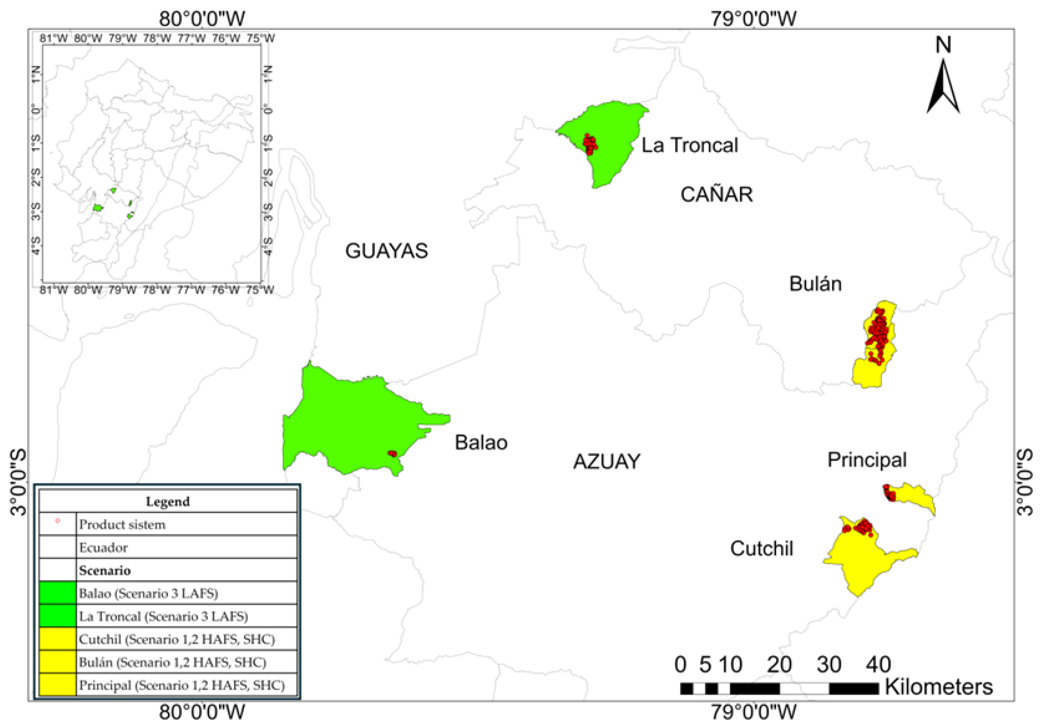
Figure 1. Diagram of the activities followed in the present investigation.
Sustainability 17 03480 g001
Figure 2. Map of Ecuador with study areas: Scenario 1: high-mountain with agroforestry systems (HAFSSs); Scenario 2: high-mountain of short-cycle crops (SHCs); and Scenario 3: low-mountain with agroforestry systems (LAFSs).
Sustainability 17 03480 g002
Figure 3. (a): cocoa agroforestry crops on gentle slopes (LAFSs) (La Troncal parish); (b): cocoa-intensive crops on flat lands (LAFSs) (Balao parish); (c): apple crops growing on steep slopes (HAFSs) (Principal parish); (d): carrot crops growing on steep slopes (SHCs) (Principal parish); (e): peach crops growing on steep slopes (HAFSs) (Bulán parish); and (f): potato crops growing on steep slopes (SHCs) (Bulán parish).
Sustainability 17 03480 g003
Figure 4. Landsat 9, Level 2, Collection 2, Tier 1, images of the study area in 2022, showing an example of the cloud cover in all the areas and seasons of the year. Photo codes from (1) to (12): months from January to December 2022, respectively.
Sustainability 17 03480 g004
Figure 5. Spearman’s correlation plot. (ac): correlations of energy inputs with SR-NVDI, TOA-NVDI, and C-NVDI, respectively; (df): correlations of energy inputs of fertilization with SR-NVDI, TOA-NVDI, and C-NVDI. [Red = high agroforestry system HAFS; Green = low agroforestry systems LAFSs; Blue = short-cycle crops SHCs].
Sustainability 17 03480 g005
Figure 6. Max_NDVI of the study area. First column (A,D,G,J): the NDVI-SR values in each of the four-year periods*; second column (B,E,H,K): the NDVI-C values in each of the four-year periods*; and third column (C,F,I,L): the NDVI-TOA values in each of the four-year periods*.
Sustainability 17 03480 g006
Figure 7. Kruskal–Wallis rank sum test (p > 0.05) for the ranges of the years 2012–2014, 2015–2017, 2018–2020, and 2021–2023 in the rows, where the study scenarios are evaluated on the x-axis and the NDVI values achieved on the y-axis. The column contains the data 1 surface reflectance (1, 4, 7, and 10), 2 composite (2, 5, 8, and 11), and 3 top of atmosphere (3, 6, 9, and 12). Each graph has the sections: (a) high-mountain, (b) low-mountain, and (c) short-cycle crops. The colors show the NDVI levels per parish in the scenarios: in green the highest values, in orange the medium values, and in red the low values.
Sustainability 17 03480 g007
Figure 8. Spearman correlation plots and linear regression (lm) equations between Landsat SR, TOA, and composite images. (a) Correlation between SR-TOA, (b) correlation between SR-composite, and (c) correlation between composite-TOA.
Sustainability 17 03480 g008
Table 1. Organization of the study, information on the scenarios, and characteristics of the production systems.
RegionScenarioParishNo. of Production Systems SampledCharacteristics
Andean HighlandsHighland agroforestry crops (HFASs)Bulán115Subsistence farming and local trade. Deciduous and annual fruit tree crops (mainly apples, pears, peaches, and avocados). Steep slopes. Altitudinal range 2265–2870 m.a.s.l. Average temperatures of 11.1 °C, and annual rainfall average of 964 mm. Managed by smallholders.
Cutchil32
Principal44
Short-cycle crops (SHCs)Bulán62Subsistence farming and local trade. Short-cycle crops (mainly corn associated with beans, squash, barley, vegetables, tree tomatoes, and potatoes). Steep slopes. Altitudinal range 2265–2870 m.a.s.l. Average temperature of 11.1 °C, and annual rainfall average 964 mm. Managed by smallholders.
Cutchil39
Principal47
Andean LowlandsLowland agroforestry crops (LFASs)La Troncal67Agriculture for local and national trade. Crops of cocoa often associated with other fruit trees, such as mangos and lemons. Gentler slopes or flat lands. Altitudinal range 90–110 m.a.s.l. Average temperature of 24.6 °C, and annual rainfall average of 1274 mm. Managed by small and medium producers.
Balao9Agriculture for local, national, and export trade. Cocoa monocultures. Flat lands. Altitudinal range 0–10 m.a.s.l. Average temperature of 24.6 °C, and annual rainfall of 1274 mm. Managed by companies.
Table 2. Number of the Landsat images that were used, from 2012 to 2023, from the TOA, SR, and composite formats (courtesy of the U.S. Geological Survey USGS).
PeriodImagen FormatNo. ImagesSensor Landsat
2021–2023TOA404Landsat 8
83Landsat 9
SR85Landsat 8
51Landsat 9
C1Landsat 7–8
2018–2020TOA294Landsat 8
SR72Landsat 8
C1Landsat 7–8
2015–2017TOA175Landsat 8
SR75Landsat 8
C1Landsat 7–8
2012–2014TOA0Landsat 5
11Landsat 7
56Landsat 8
0Landsat 5
SR11Landsat 7
39Landsat 8
C1Landsat 7–8
Table 4. Energy input sources in the studied scenarios, and their average distribution in GJ ha−1, and percentages.
HAFSLAFSSHCTotal
Mean%Mean%Mean%Mean%
Work1.7526.302.2419.906.7620.506.2421.60
Fertilizers3.1547.408.5876.3012.8939.0016.0255.46
Pesticides0.6710.100.423.802.256.801.846.38
Vegetal issues1.0115.200.000.0010.8032.704.6115.95
Irrigation water0.071.000.000.000.321.000.180.61
Tot Inputs6.65100.0011.24100.0033.01100.0028.89100.00
Table 5. Table of the disaggregated inputs used in the studied production systems, with their values expressed in GJ ha−1.
TotalWorkFertilizerPesticideVegetal issuesIrrigation water
GJ ha−12498.914066.56640.522090.6068.41
InputsHumanAnimalMachineFuelSyntheticOrganicInsect.Fung.Herb.SeedsPlantsIrrigation water
GJ ha−1723.8099.6161.851613.642711.151355.40142.58376.08121.852014.0076.6068.41
%28.963.992.4864.5766.6733.3322.2658.7219.0296.343.66100
Table 6. Kruskal–Wallis rank sum test of type system with SR, TOA, composite images. The letters (a, b, ab, etc.) indicate statistical significance based on multiple comparison tests.
NDVI Image
SystemSR_Meansdp-ValueRangeComp_Meansdp-ValueRangeTOA_Meansdp-ValueRange
LAFS0.850.052.20 × 10−6a0.760.098.57 × 10−11a0.680.080.08ab
HAFS0.790.08b0.670.08b0.690.06b
SHC0.790.08b0.660.11b0.690.08a
Disclaimer/Publisher’s Note: The statements, opinions and data contained in all publications are solely those of the individual author(s) and contributor(s) and not of MDPI and/or the editor(s). MDPI and/or the editor(s) disclaim responsibility for any injury to people or property resulting from any ideas, methods, instructions or products referred to in the content.

