

Enhanced Fault Detection and Classification in AC Microgrids Through a Combination of Data Processing Techniques and Deep Neural Networks

Abstract
1. Introduction
2. Problem Formulation
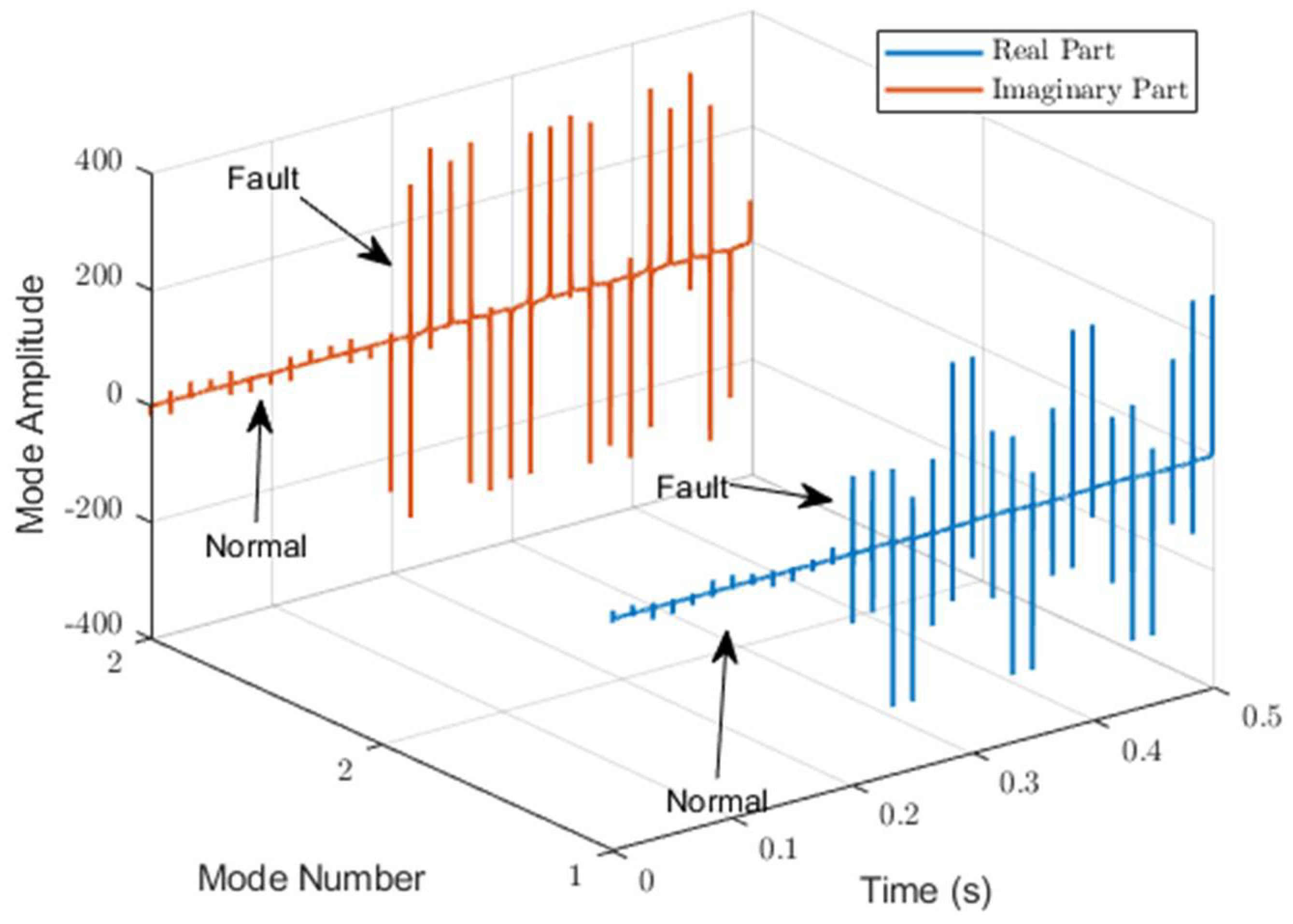
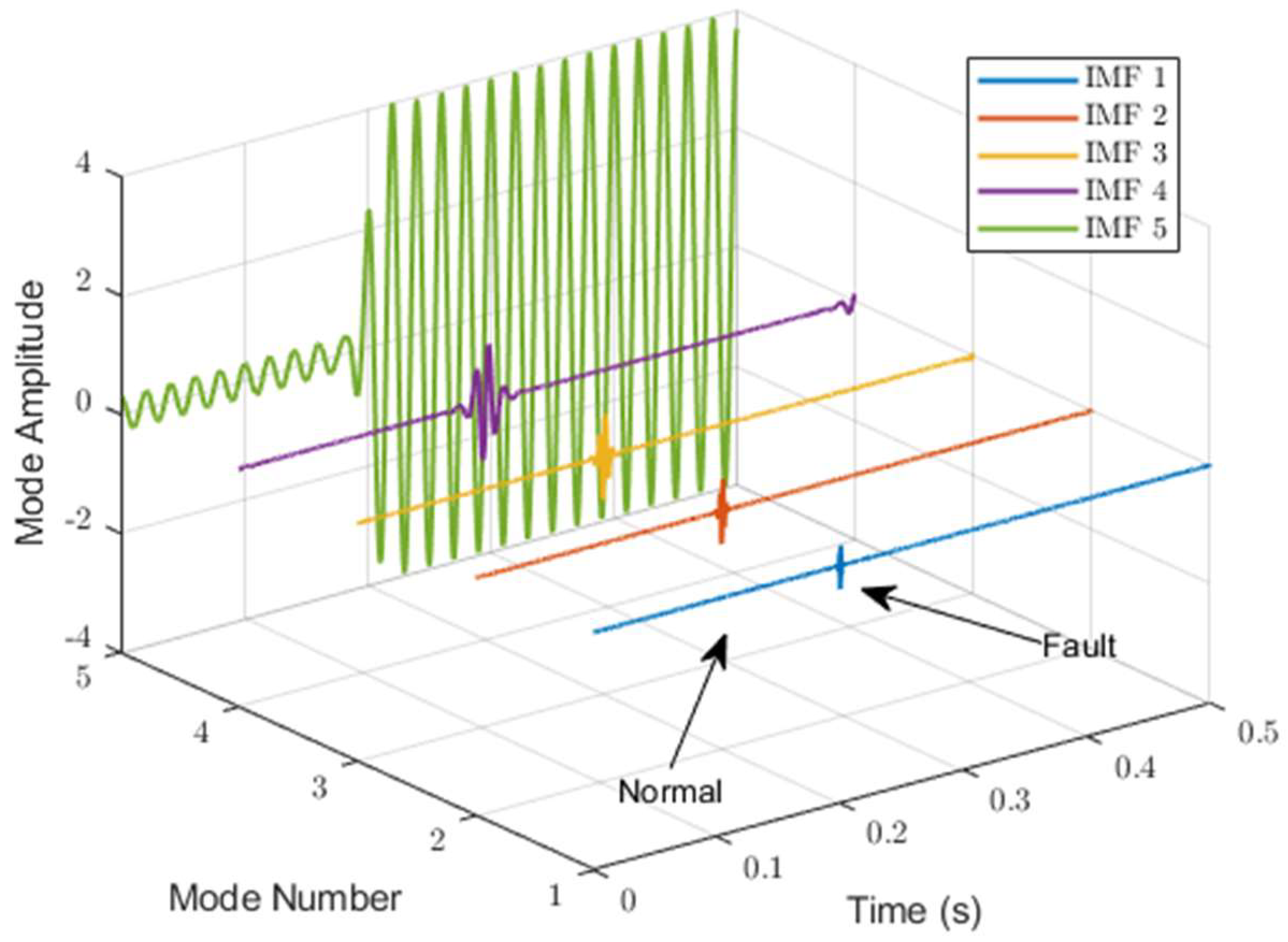
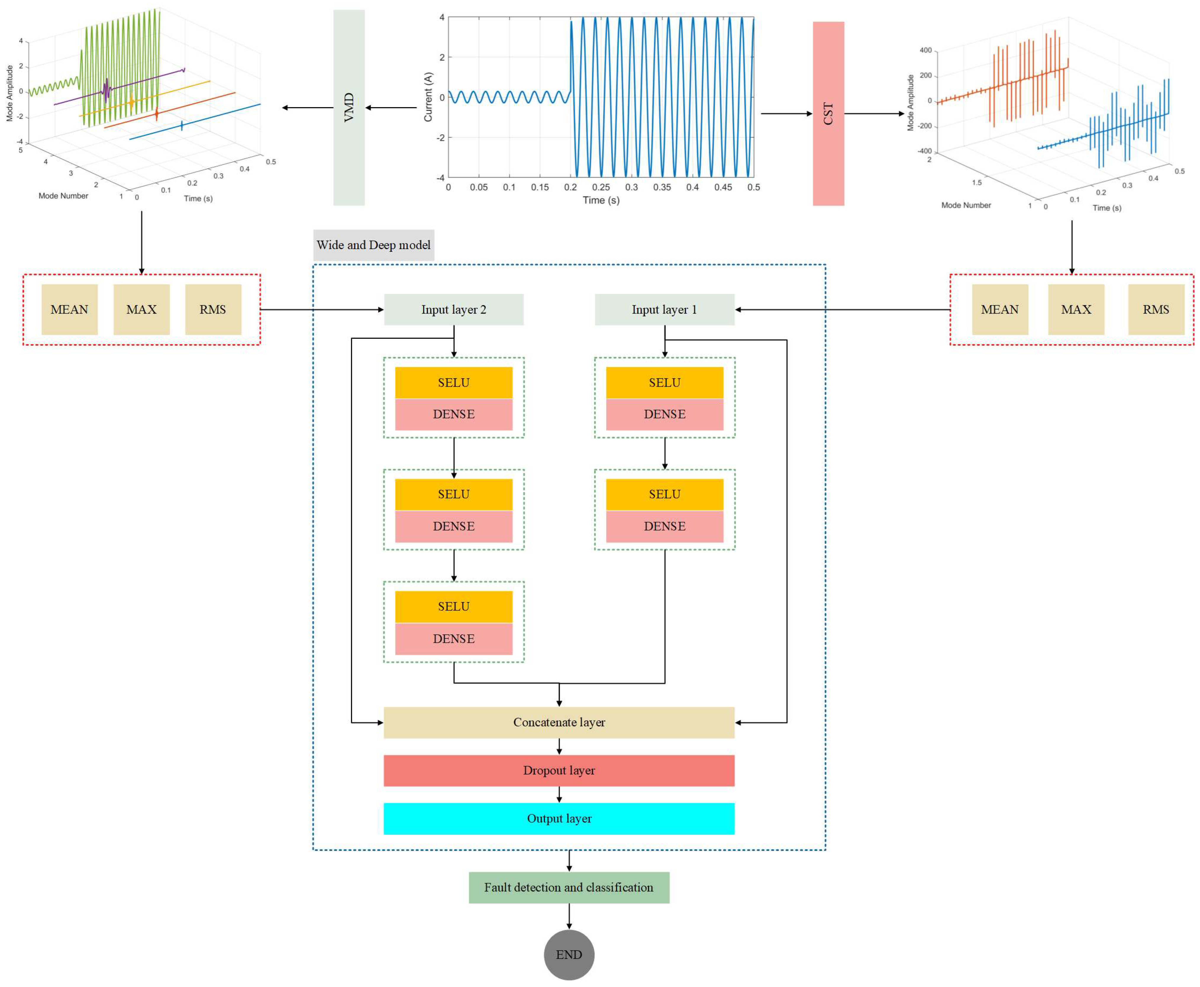
2.1. Feature Exctraction
2.2. Proposed WDL Model
| Algorithm 1: Fault Classification in AC Microgrids Using Signal Processing and Deep Learning | ||||
| Input: | : Current signal of the microgrid. | |||
| Output: | : Softmax probability vector for 11 fault classes. | |||
| Algorithm Steps: | ||||
| 1. Signal Processing and Feature Extraction: | ||||
| : | ||||
| into IMFs | ||||
| : | ||||
| Extract real and image features using CST. | ||||
| 1.3. Compute statistical features for both VMD and CST outputs: | ||||
| Mean, RMS, and MAX. | ||||
| and | ||||
| Split the dataset into training (70%) and testing (30%) subsets. | ||||
| Further split the training data into training (70%) and validation (30%) subsets. | ||||
| 2. Input Layers: | ||||
| 2.1. Define two input layers: | ||||
| 3. Branch 1 (VMD Feature Processing): | ||||
| 3.1. Dense layer (100 units, SELU, L2 regularization)→Batch Normalization. | ||||
| 3.2. Dense layer (50 units, SELU, L2 regularization)→Batch Normalization. | ||||
| 3.3. Dense layer (25 units, SELU, L2 regularization). | ||||
| 4. Branch 2 (CST Feature Processing): | ||||
| 4.1. Dense layer (50 units, SELU, L2 regularization)→Batch Normalization. | ||||
| 4.2. Dense layer (25 units, SELU, L2 regularization). | ||||
| 5. Feature Concatenation: | ||||
| 6. Regularization: | ||||
| 6.1. Apply Dropout with a rate of 0.1 to the concatenated features. | ||||
| 7. Output Layer: | ||||
| 7.1. Dense layer with 11 units and softmax activation to produce class probabilities. | ||||
| 8. Training and Validation: | ||||
| 8.1. Train the model using the training subset (70% of the total data). | ||||
| 8.2. Use the validation subset (30% of the training data) for hyperparameter tuning and monitoring. | ||||
| 9. Testing: | ||||
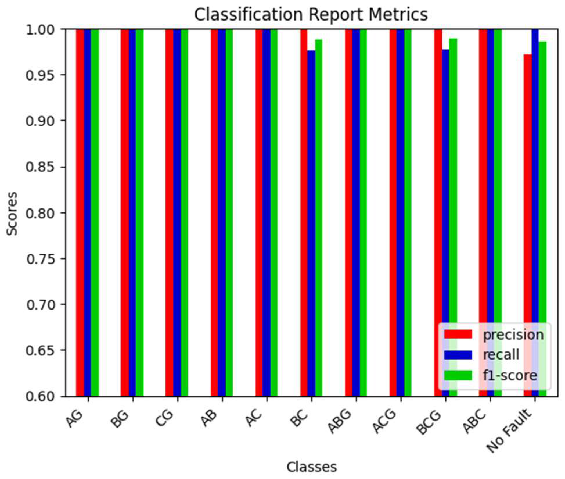
| 9.1. Evaluate the trained model on the test subset (30% of the total data) to assess performance metrics such as accuracy, precision, recall, and F1-score. | ||||
3. Simulation Results
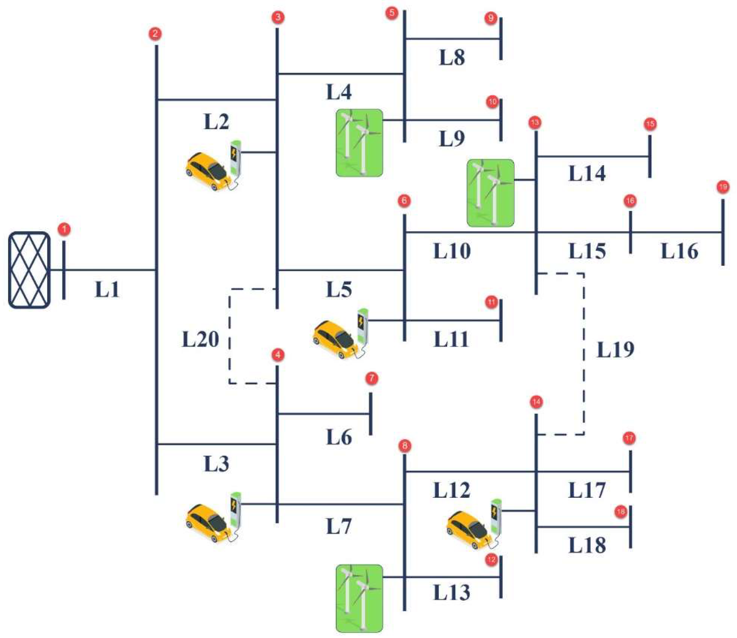
3.1. Case Study
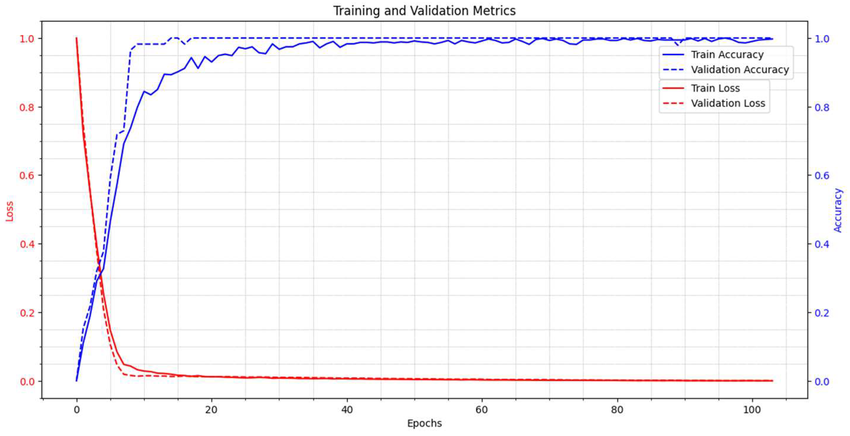
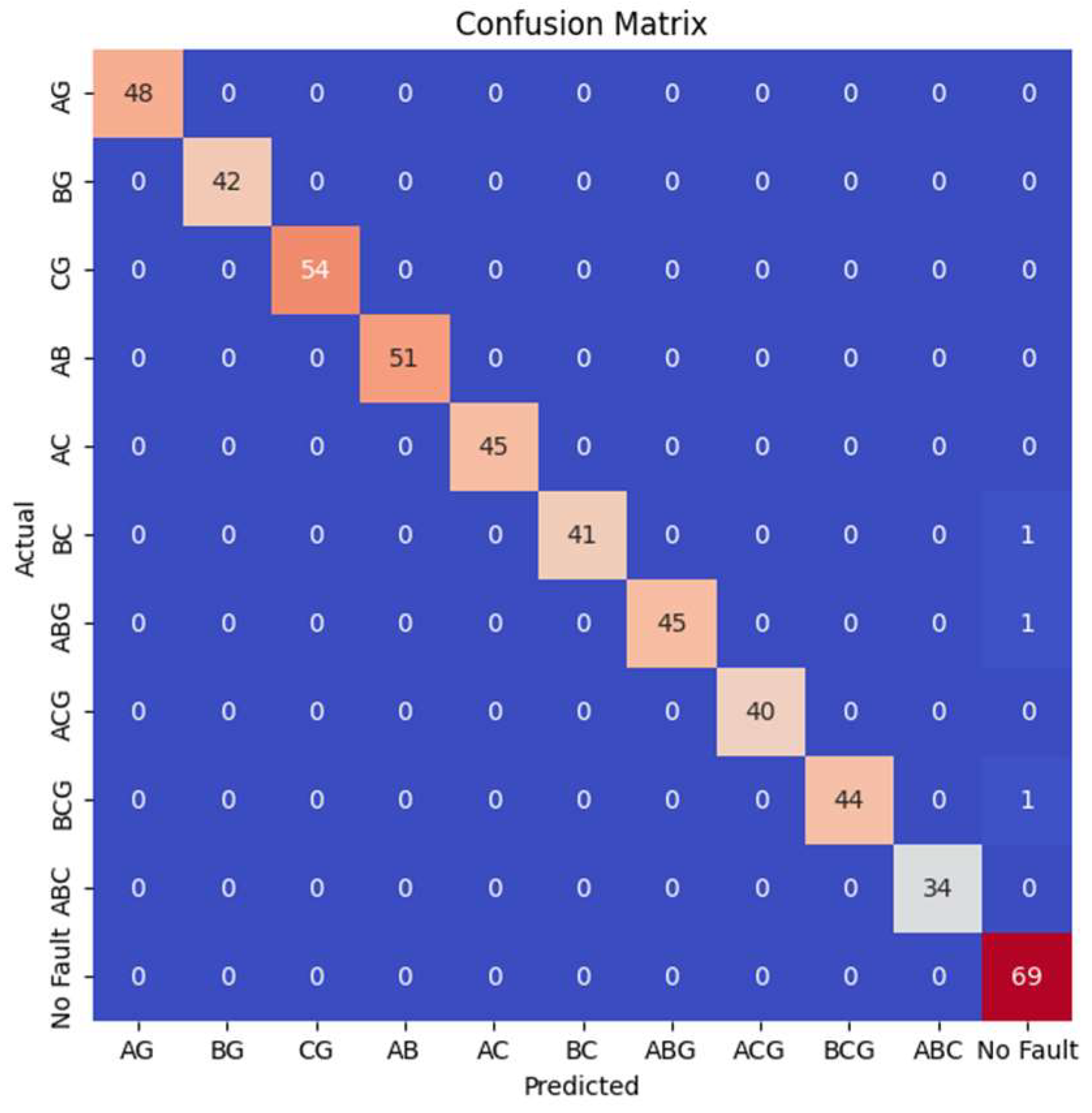
3.2. Accuracy of the Proposed Method When Protecting the L9 Line
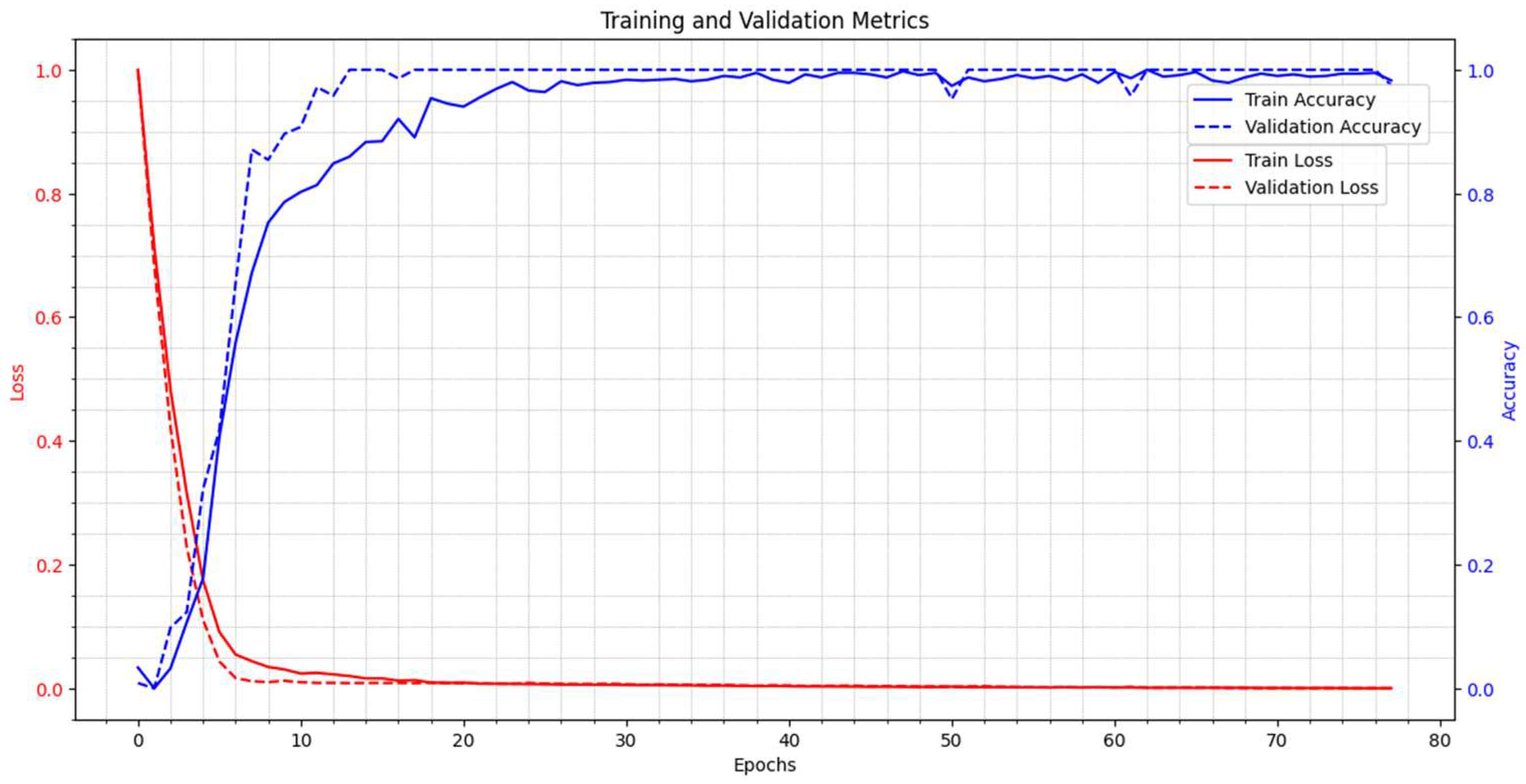
3.3. Accuracy of the Proposed Method When Protecting the L10 Line
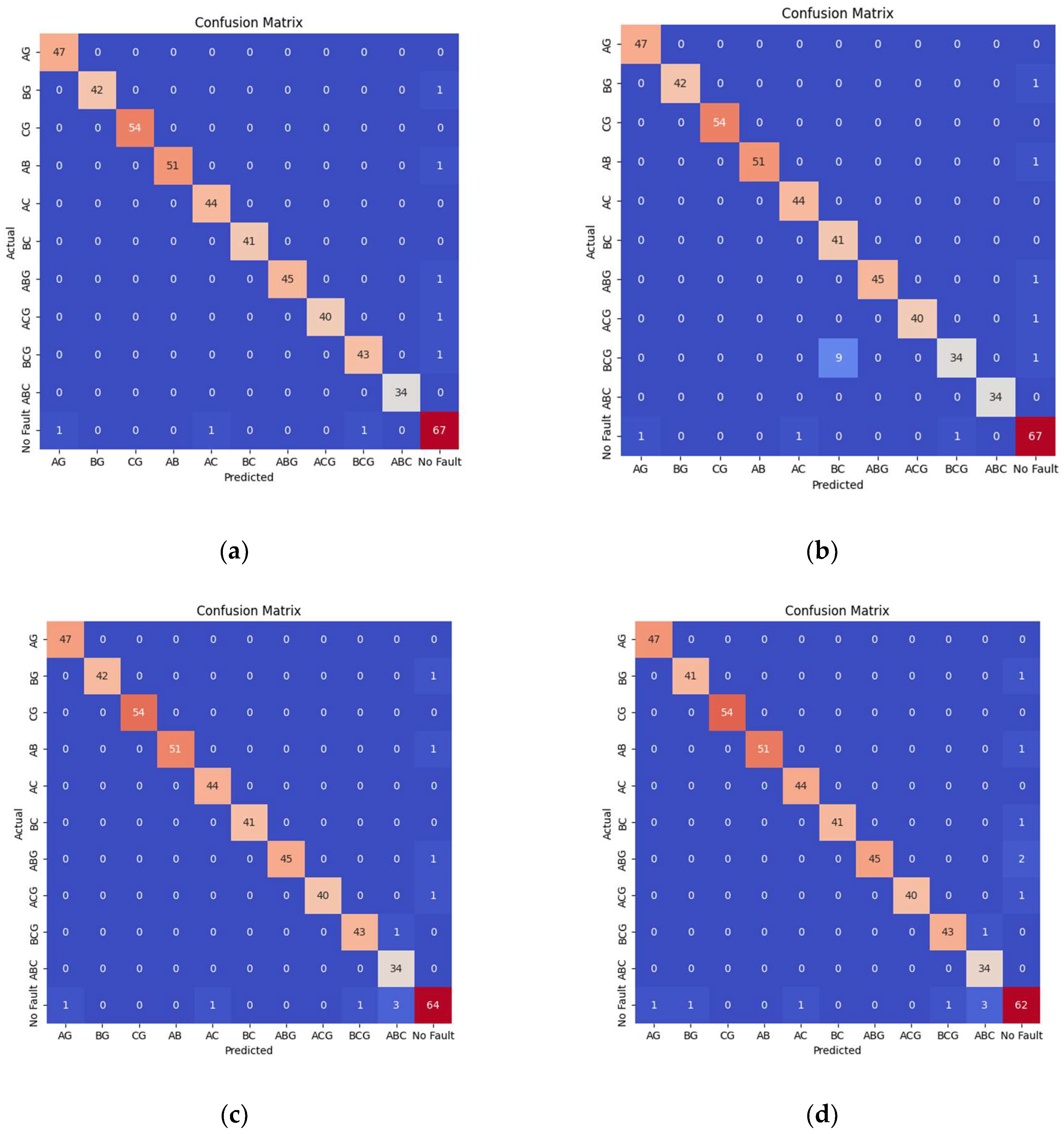
4. Performance Comparison of the Proposed Approach
4.1. Comparison with Alternative Intelligent Methods
4.2. Comparison with Alternative Methods Discussed in Studies
5. Conclusions
Author Contributions
Funding
Institutional Review Board Statement
Informed Consent Statement
Data Availability Statement
Conflicts of Interest
References
- Tao, L.; Schwaegerl, C.; Narayanan, S.; Zhang, J.H. From laboratory Microgrid to real markets—Challenges and opportunities. In Proceedings of the 2011 IEEE 8th International Conference on Power Electronics and ECCE Asia (ICPE & ECCE), Jeju, Republic of Korea, 30 May–3 June 2011; pp. 264–271. [Google Scholar]
- Pradhan, R.; Jena, P. An innovative fault direction estimation technique for AC microgrid. Electr. Power Syst. Res. 2023, 215, 108997. [Google Scholar] [CrossRef]
- Zarei, S.F.; Khankalantary, S. Protection of active distribution networks with conventional and inverter-based distributed generators. Int. J. Electr. Power Energy Syst. 2021, 129, 106746. [Google Scholar] [CrossRef]
- Hussain, N.; Nasir, M.; Vasquez, J.C.; Guerrero, J.M. Recent Developments and Challenges on AC Microgrids Fault Detection and Protection Systems—A Review. Energies 2020, 13, 2149. [Google Scholar] [CrossRef]
- Rashid, U.; Dhillon, J. Transients Analysis in AC Microgrid System. J. Phys. Conf. Ser. 2022, 2327, 012009. [Google Scholar] [CrossRef]
- Sharma, S.; Tripathy, M.; Wang, L. A novel fault detection and classification scheme for DC microgrid based on transient reactor voltage with localized back-up scheme. Int. J. Electr. Power Energy Syst. 2022, 142, 108275. [Google Scholar] [CrossRef]
- Tailor, J.K.; Osman, A.H. Restoration of fuse-recloser coordination in distribution system with high DG penetration. In Proceedings of the Power and Energy Society General Meeting—Conversion and Delivery of Electrical Energy in the 21st Century, Pittsburgh, PA, USA, 20–24 July 2008; pp. 1–8. [Google Scholar]
- Beheshtaein, S.; Cuzner, R.M.; Forouzesh, M.; Savaghebi, M.; Guerrero, J.M. DC Microgrid Protection: A Comprehensive Review. IEEE J. Emerg. Sel. Top. Power Electron. 2019, 1. [Google Scholar] [CrossRef]
- Al-Nasseri, H.; Redfern, M.A.; Li, F. A voltage based protection for micro-grids containing power electronic converters. In Proceedings of the Power Engineering Society General Meeting, Montreal, QC, Canada, 18–22 June 2006; p. 7. [Google Scholar]
- Singh, M.; Basak, P. Adaptive protection methodology in microgrid for fault location and nature detection using q0 components of fault current. IET Gener. Transm. Distrib. 2019, 13, 760–769. [Google Scholar] [CrossRef]
- Zamani, M.A.; Sidhu, T.S.; Yazdani, A. A Protection Strategy and Microprocessor-Based Relay for Low-Voltage Microgrids. Power Deliv. IEEE Trans. 2011, 26, 1873–1883. [Google Scholar] [CrossRef]
- El-Zonkoly, A.M. Fault diagnosis in distribution networks with distributed generation. Electr. Power Syst. Res. 2011, 81, 1482–1490. [Google Scholar] [CrossRef]
- Abo-Ahmed, P.-l.; Ahshan, R.; Abu-Khaizaran, M.; Alsayid, B.; Rahman, M. Implementing and Testing d−q WPT-Based Digital Protection for Micro-Grid Systems. IEEE Trans. Ind. Appl. 2014, 50, 2173–2185. [Google Scholar] [CrossRef]
- Abdelgayed, T.S.; Morsi, W.G.; Sidhu, T.S. A New Approach for Fault Classification in Microgrids Using Optimal Wavelet Functions Matching Pursuit. IEEE Trans. Smart Grid 2018, 9, 4838–4846. [Google Scholar] [CrossRef]
- Zheng, X.; Zeng, Y.; Zhao, M.; Venkatesh, B. Early Identification and Location of Short-Circuit Fault in Grid-Connected AC Microgrid. IEEE Trans. Smart Grid 2021, 12, 2869–2878. [Google Scholar] [CrossRef]
- Huang, H.; Gong, Z.; Shu, H.; Tian, X. Microgrid Fault Detection Method Based on Sequential Overlapping Differential Transform. In Proceedings of the 2020 IEEE 4th Conference on Energy Internet and Energy System Integration (EI2), Wuhan, China, 30 October–1 November 2020; pp. 2308–2313. [Google Scholar]
- Samantaray, S.R.; Joos, G.; Kamwa, I. Differential energy based microgrid protection against fault conditions. In Proceedings of the Innovative Smart Grid Technologies (ISGT), Washington, DC, USA, 16–20 January 2012; pp. 1–7. [Google Scholar]
- Gururani, A.; Mohanty, S.R.; Mohanta, J.C. Microgrid protection using Hilbert–Huang transform based-differential scheme. IET Gener. Transm. Distrib. 2016, 10, 3707–3716. [Google Scholar] [CrossRef]
- Dharmapandit, O.; Patnaik, R.K.; Dash, P.K. A Fast Time-Frequency Response Based Differential Spectral Energy Protection of AC Microgrids Including Fault Location. Prot. Control Mod. Power Syst. 2017, 2, 1–28. [Google Scholar] [CrossRef]
- Al-Nasseri, H.; Redfern, M.A. Harmonics content based protection scheme for Micro-grids dominated by solid state converters. In Proceedings of the 2008 12th International Middle-East Power System Conference, MEPCON 2008, Aswan, Egypt, 12–15 March 2008; pp. 50–56. [Google Scholar]
- Petit, M.; Le Pivert, X.; Garcia-Santander, L. Directional relays without voltage sensors for distribution networks with distributed generation: Use of symmetrical components. Electr. Power Syst. Res. 2010, 80, 1222–1228. [Google Scholar] [CrossRef]
- Pinto, J.O.C.P.; Moreto, M. Protection strategy for fault detection in inverter-dominated low voltage AC microgrid. Electr. Power Syst. Res. 2021, 190, 106572. [Google Scholar] [CrossRef]
- Zhang, F.; Mu, L. New protection scheme for internal fault of multi-microgrid. Prot. Control Mod. Power Syst. 2019, 4, 14. [Google Scholar] [CrossRef]
- Dong, X.; Shi, S. Identifying Single-Phase-to-Ground Fault Feeder in Neutral Noneffectively Grounded Distribution System Using Wavelet Transform. IEEE Trans. Power Deliv. 2008, 23, 1829–1837. [Google Scholar] [CrossRef]
- Deshmukh, B.; Kumar Lal, D.; Biswal, S. A reconstruction based adaptive fault detection scheme for distribution system containing AC microgrid. Int. J. Electr. Power Energy Syst. 2023, 147, 108801. [Google Scholar] [CrossRef]
- Srivastava, A.; Parida, S.K. Data driven approach for fault detection and Gaussian process regression based location prognosis in smart AC microgrid. Electr. Power Syst. Res. 2022, 208, 107889. [Google Scholar] [CrossRef]
- Zaben, M.M.; Worku, M.Y.; Hassan, M.A.; Abido, M.A. Machine Learning Methods for Fault Diagnosis in AC Microgrids: A Systematic Review. IEEE Access 2024, 12, 20260–20298. [Google Scholar] [CrossRef]
- Hosseini, S.A.; Askarian Abyaneh, H.; Sadeghi, S.H.H.; Eslami, R. Improving Adaptive Protection to Reduce Sensitivity to Uncertainties Which Affect Protection Coordination of Microgrids. Iran. J. Sci. Technol. Trans. Electr. Eng. 2018, 42, 63–74. [Google Scholar] [CrossRef]
- Aiswarya, R.; Nair, D.S.; Rajeev, T.; Vinod, V. A novel SVM based adaptive scheme for accurate fault identification in microgrid. Electr. Power Syst. Res. 2023, 221, 109439. [Google Scholar] [CrossRef]
- Mbey, C.F.; Foba Kakeu, V.J.; Boum, A.T.; Souhe, F.G.Y. Fault detection and classification using deep learning method and neuro-fuzzy algorithm in a smart distribution grid. J. Eng. 2023, 2023, e12324. [Google Scholar] [CrossRef]
- Hadaeghi, A.; Samet, H.; Ghanbari, T. Multi extreme learning machine approach for fault location in multi-terminal high-voltage direct current systems. Comput. Electr. Eng. 2019, 78, 313–327. [Google Scholar] [CrossRef]
- Gangwar, A.K.; Shaik, A.G. k-Nearest neighbour based approach for the protection of distribution network with renewable energy integration. Electr. Power Syst. Res. 2023, 220, 109301. [Google Scholar] [CrossRef]
- Srivastava, A.; Kumar, A.; Kumar, A.; Sriharsh, S.; Parida, S.K.; Priyadarshi, H. Random Forest based Fault Detection and Localization in Microgrid using Simplified Measurements. In Proceedings of the 2023 IEEE IAS Global Conference on Emerging Technologies (GlobConET), London, UK, 19–21 May 2023; pp. 1–6. [Google Scholar]
- Xu, Y.; Zhou, Y.; Sekula, P.; Ding, L. Machine learning in construction: From shallow to deep learning. Dev. Built Environ. 2021, 6, 100045. [Google Scholar] [CrossRef]
- Bramareswara Rao, S.; Kumar, Y.P.; Amir, M.; Muyeen, S. Fault detection and classification in hybrid energy-based multi-area grid-connected microgrid clusters using discrete wavelet transform with deep neural networks. Electr. Eng. 2024, 1–18. [Google Scholar] [CrossRef]
- James, J.; Hou, Y.; Lam, A.Y.; Li, V.O. Intelligent fault detection scheme for microgrids with wavelet-based deep neural networks. IEEE Trans. Smart Grid 2017, 10, 1694–1703. [Google Scholar]
- Nazari, A.A.; Hosseini, S.A.; Taheri, B. Improving the performance of differential relays in distinguishing between high second harmonic faults and inrush current. Electr. Power Syst. Res. 2023, 223, 109675. [Google Scholar] [CrossRef]
- Dragomiretskiy, K.; Zosso, D. Variational Mode Decomposition. IEEE Trans. Signal Process. 2014, 62, 531–544. [Google Scholar] [CrossRef]
- Taheri, B.; Sedighizadeh, M. Detection of power swing and prevention of mal-operation of distance relay using compressed sensing theory. IET Gener. Transm. Distrib. 2020, 14, 5558–5570. [Google Scholar] [CrossRef]
- Salehimehr, S.; Miraftabzadeh, S.M.; Brenna, M. A Novel Machine Learning-Based Approach for Fault Detection and Location in Low-Voltage DC Microgrids. Sustainability 2024, 16, 2821. [Google Scholar] [CrossRef]
- Rani, M.; Dhok, S.B.; Deshmukh, R.B. A Systematic Review of Compressive Sensing: Concepts, Implementations and Applications. IEEE Access 2018, 6, 4875–4894. [Google Scholar] [CrossRef]
- Baraniuk, R.G. Compressive Sensing [Lecture Notes]. IEEE Signal Process. Mag. 2007, 24, 118–121. [Google Scholar] [CrossRef]
- Candes, E.J.; Wakin, M.B. An Introduction To Compressive Sampling. IEEE Signal Process. Mag. 2008, 25, 21–30. [Google Scholar] [CrossRef]
- Xiang, H.L.a.J. Autoregressive model-enhanced variational mode decomposition for mechanical fault detection. IET Sci. Meas. Technol. 2019, 13, 843–851. [Google Scholar]
- Ghotbi-Maleki, M.; Chabanloo, R.M.; Zeineldin, H.H.; Miangafsheh, S.M.H. Design of Setting Group-Based Overcurrent Protection Scheme for Active Distribution Networks Using MILP. IEEE Trans. Smart Grid 2021, 12, 1185–1193. [Google Scholar] [CrossRef]
- Mohammadi Chabanloo, R.; Ghotbi Maleki, M. An accurate method for overcurrent–distance relays coordination in the presence of transient states of fault currents. Electr. Power Syst. Res. 2018, 158, 207–218. [Google Scholar] [CrossRef]
- Yang, X.; Yang, L.; Xiao, X.; Wang, Y.; Zhang, S. An adaptive lightweight seq2subseq model for non-intrusive load monitoring. IET Gener. Transm. Distrib. 2022, 16, 3706–3718. [Google Scholar] [CrossRef]
- Hosseini, S.A.; Taheri, B.; Sadeghi, S.H.H.; Nasiri, A. A Deep Learning Model for Fault Detection in Distribution Networks with High Penetration of Electric Vehicle Chargers. e-Prime-Adv. Electr. Eng. Electron. Energy 2024, 10, 100845. [Google Scholar] [CrossRef]
- Liu, Y.; Zhang, S.; Li, L.; Wang, S.; Lu, T.; Yu, H.; Liu, W. A machine learning-based fault identification method for microgrids with distributed generations. J. Phys. Conf. Ser. 2022, 2360, 012019. [Google Scholar] [CrossRef]
- Cano, A.; Arévalo, P.; Benavides, D.; Jurado, F. Integrating discrete wavelet transform with neural networks and machine learning for fault detection in microgrids. Int. J. Electr. Power Energy Syst. 2024, 155, 109616. [Google Scholar] [CrossRef]
- Basher, B.G.; Ghanem, A.; Abulanwar, S.; Hassan, M.K.; Rizk, M.E. Fault classification and localization in microgrids: Leveraging discrete wavelet transform and multi-machine learning techniques considering single point measurements. Electr. Power Syst. Res. 2024, 231, 110362. [Google Scholar] [CrossRef]


| Parameters | Details |
|---|---|
| Inputs | Input_1 (VMD), Input_2 (CST) |
| Branch 1 | Dense: 100 Hidden Layers, Activation: SELU |
| Dense: 50 Hidden Layers, Activation: SELU | |
| Dense: 25 Hidden Layers, Activation: SELU | |
| Branch 2 | Dense: 50 Hidden Layers, Activation: SELU |
| Dense: 25 Hidden Layers, Activation: SELU | |
| Dropout | 10% |
| Output | Dense: 11 Hidden Layers, Activation: Softmax |
| Optimizer | Adam |
| Loss function | Sparse categorical crossentropy |
| Metric | Accuracy |
| Epochs | 500 |
| Batch size | 32 |
| Callbacks | Early stopping |
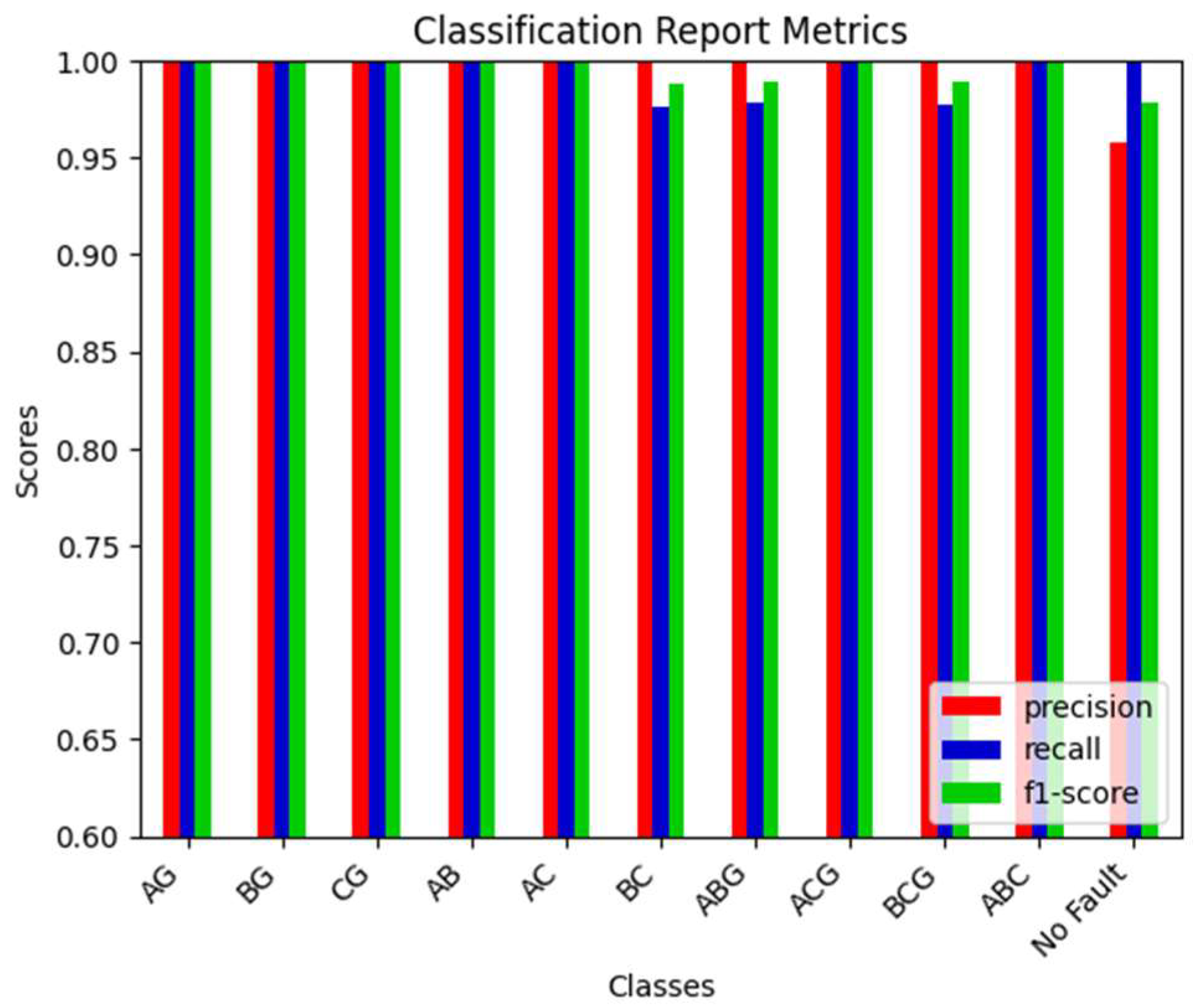
| Case | Proposed Method | KNN | SVM | RF | XGBOOST | ||||||||||
|---|---|---|---|---|---|---|---|---|---|---|---|---|---|---|---|
| PR * | RE ** | F1 | PR | RE | F1 | PR | RE | F1 | PR | RE | F1 | PR | RE | F1 | |
| AG | 1 | 1 | 1 | 0.98 | 1 | 0.99 | 0.98 | 1 | 0.99 | 0.98 | 1 | 0.99 | 0.98 | 1 | 0.99 |
| BG | 1 | 1 | 1 | 1 | 0.98 | 0.99 | 1 | 0.98 | 0.99 | 1 | 0.98 | 0.99 | 0.98 | 0.98 | 0.98 |
| CG | 1 | 1 | 1 | 1 | 1 | 1 | 1 | 1 | 1 | 1 | 1 | 1 | 1 | 1 | 1 |
| AB | 1 | 1 | 1 | 1 | 0.98 | 0.99 | 1 | 0.98 | 0.99 | 1 | 0.98 | 0.99 | 1 | 0.98 | 0.99 |
| AC | 1 | 1 | 1 | 0.98 | 1 | 0.99 | 0.98 | 1 | 0.99 | 0.98 | 1 | 0.99 | 0.98 | 1 | 0.99 |
| BC | 1 | 0.98 | 0.99 | 1 | 1 | 1 | 0.82 | 1 | 0.9 | 1 | 1 | 1 | 1 | 0.98 | 0.99 |
| ABG | 1 | 1 | 1 | 1 | 0.98 | 0.99 | 1 | 0.98 | 0.99 | 1 | 0.98 | 0.99 | 1 | 0.96 | 0.98 |
| ACG | 1 | 1 | 1 | 1 | 0.98 | 0.99 | 1 | 0.98 | 0.99 | 1 | 0.98 | 0.99 | 1 | 0.98 | 0.99 |
| BCG | 1 | 0.98 | 0.99 | 0.98 | 0.98 | 0.98 | 0.97 | 0.77 | 0.86 | 0.98 | 0.98 | 0.98 | 0.98 | 0.98 | 0.98 |
| ABC | 1 | 1 | 1 | 1 | 1 | 1 | 1 | 1 | 1 | 0.89 | 1 | 0.94 | 0.89 | 1 | 0.94 |
| No fault | 0.97 | 1 | 0.99 | 0.93 | 0.96 | 0.94 | 0.93 | 0.96 | 0.94 | 0.94 | 0.91 | 0.93 | 0.91 | 0.9 | 0.91 |
| Ref. | Feature Extraction Method | Intelligent Model | Microgrid Topology Uncertainty | Distinction Between Permanent Faults and Transient Waves | Fault Detection | Fault Classification | Wind | EV |
|---|---|---|---|---|---|---|---|---|
| [35] | Discrete wavelet transform | DNN | ✓ | ✓ | ✓ | ✓ | ✗ | ✗ |
| [36] | Discrete wavelet transform | GRU | ✓ | ✓ | ✓ | ✓ | ✗ | ✗ |
| [48] | 2D modeling | BWO-BiLSTM | ✓ | ✓ | ✓ | ✗ | ✗ | ✓ |
| [49] | FP-growth-K-means-mini-batch gradient descent | ✗ | ✗ | ✓ | ✗ | ✗ | ✗ | |
| [50] | Discrete wavelet transform | RBFNN neuronal network | ✓ | ✗ | ✓ | ✓ | ✗ | ✗ |
| [51] | Discrete wavelet transform | DT | ✓ | ✓ | ✓ | ✓ | ✗ | ✗ |
| Proposed method | CST-VMD | WDL | ✓ | ✓ | ✓ | ✓ | ✓ | ✓ |
Disclaimer/Publisher’s Note: The statements, opinions and data contained in all publications are solely those of the individual author(s) and contributor(s) and not of MDPI and/or the editor(s). MDPI and/or the editor(s) disclaim responsibility for any injury to people or property resulting from any ideas, methods, instructions or products referred to in the content. |
© 2025 by the authors. Licensee MDPI, Basel, Switzerland. This article is an open access article distributed under the terms and conditions of the Creative Commons Attribution (CC BY) license (https://creativecommons.org/licenses/by/4.0/).
Share and Cite
Taheri, B.; Hosseini, S.A.; Hashemi-Dezaki, H. Enhanced Fault Detection and Classification in AC Microgrids Through a Combination of Data Processing Techniques and Deep Neural Networks. Sustainability 2025, 17, 1514. https://doi.org/10.3390/su17041514
Taheri B, Hosseini SA, Hashemi-Dezaki H. Enhanced Fault Detection and Classification in AC Microgrids Through a Combination of Data Processing Techniques and Deep Neural Networks. Sustainability. 2025; 17(4):1514. https://doi.org/10.3390/su17041514
Chicago/Turabian StyleTaheri, Behrooz, Seyed Amir Hosseini, and Hamed Hashemi-Dezaki. 2025. "Enhanced Fault Detection and Classification in AC Microgrids Through a Combination of Data Processing Techniques and Deep Neural Networks" Sustainability 17, no. 4: 1514. https://doi.org/10.3390/su17041514
APA StyleTaheri, B., Hosseini, S. A., & Hashemi-Dezaki, H. (2025). Enhanced Fault Detection and Classification in AC Microgrids Through a Combination of Data Processing Techniques and Deep Neural Networks. Sustainability, 17(4), 1514. https://doi.org/10.3390/su17041514