Spatiotemporal Evolution and Driving Factors of Coupling Coordination Between Carbon Emission Efficiency and Carbon Balance in the Yellow River Basin

Abstract

This study investigates the coupling coordination between carbon emission efficiency (CEE) and carbon balance (CB) in the Yellow River Basin (YRB), aiming to support high-quality regional development and the realization of China’s “dual carbon” goals. Based on panel data from 74 cities in the YRB between 2006 and 2022, the Super-SBM model, Ecological Support Coefficient (ESC), and coupling coordination degree (CCD) model are applied to evaluate the synergy between CEE and CB. Spatiotemporal patterns and driving mechanisms are analyzed using kernel density estimation, Moran’s I index, the Dagum Gini coefficient, Markov chains, and the XGBoost algorithm. The results reveal a generally low and declining level of CCD, with the upstream and midstream regions performing better than the downstream. Spatial clustering is evident, characterized by significant positive autocorrelation and high-high or low-low clusters. Although regional disparities in CCD have narrowed slightly over time, interregional differences remain the primary source of variation. The likelihood of leapfrog development in CCD is limited, and high-CCD regions exhibit weak spillover effects. Forest coverage is identified as the most critical driver, significantly promoting CCD. Conversely, population density, urbanization, energy structure, and energy intensity negatively affect coordination. Economic development demonstrates a U-shaped relationship with CCD. Moreover, nonlinear interactions among forest coverage, population density, energy structure, and industrial enterprise scale further intensify the complexity of CCD. These findings provide important implications for enhancing regional carbon governance and achieving balanced ecological-economic development in the YRB.

1. Introduction

Since the Industrial Revolution, the rapid expansion of energy-intensive industries has led to a steady rise in carbon emissions (CEs), intensifying the conflict between human development and carbon balance (CB). In 2024, global anthropogenic CEs reached a record high of 11.3 GtC, posing increasing risks to both human well-being and ecological sustainability. To address the tension between high-efficiency economic growth and the need to enhance CB, in 2015, the United Nations established a set of 17 Sustainable Development Goals (SDGs) designed to address pressing environmental, social, and economic challenges worldwide. These goals provide a comprehensive framework for coordinated international efforts spanning the period from 2015 to 2030. SDG 7 (“Affordable and Clean Energy”), SDG 11 (“Sustainable Cities and Communities”), and SDG 13 (“Climate Action”) reflect the international commitment to carbon reduction.

As the largest contributor to global carbon emissions, China has committed to reaching its emissions peak by 2030 and attaining carbon neutrality by 2060. The YRB, a critical hub for China’s mineral resources, has experienced rapid economic growth in recent decades—growth that has come at a significant environmental cost. Accelerated industrialization and urbanization have led to a high population density, increased energy consumption, and substantial ecological degradation. These developments have not only intensified urban CEs but also weakened the carbon sink (CS) capacity of local ecosystems, undermining the country’s dual carbon goals. Therefore, cities in the YRB face the dual tasks of carbon reduction and carbon neutrality. It is thus essential to improve the CEE and maintain CB.

CEE refers to an economy’s ability to generate maximum economic output and minimum CEs with minimal resource consumption [1]. It is widely used to measure the level of low-carbon economic development and carbon reduction capacity in a region. Improving the CEE can enhance energy use efficiency, reduce CEs, and promote high-quality economic development [2,3]. However, due to the carbon rebound effect, China is still experiencing a simultaneous increase in CEE and total CEs [4]. As a result, CEE alone cannot fully reflect the trend toward carbon neutrality. CB, defined as the balance between CS and CEs within a specific region and time, offers a more objective and comprehensive indicator of carbon neutrality [5]. Yet, as a single indicator, CB mainly reflects ecological carrying capacity and does not capture the efficiency of low-carbon economic development. Therefore, it is necessary to establish a more comprehensive framework that integrates both CEE and CB. Achieving effective coordination between the two is essential for promoting high-quality economic development and advancing the dual carbon goals in the YRB.

The CCD between CEE and CB has not yet received widespread attention. Although existing studies have made significant progress in examining CEE and CB separately, most focus on the impact of individual factors. For the CEE, research has mainly explored the effects of digital economic development, industrial clusters, and advancement in green technology [2,6,7]. For the CB, studies have examined how industrial upgrading, ecological construction, and urbanization trade-offs influence CB [8,9]. Regarding the relationship between CEE and CB, the current literature primarily addresses the link between CEE and the ecological environment, suggesting that improvements in CEE can promote environmental quality, while environmental improvements may constrain CEE [10]. However, these perspectives are limited in explaining the coupling between CEE and CB and fail to reveal the internal interaction mechanisms between low-carbon development and carbon neutrality goals.

Against this background, this study aims to systematically analyze the CCD between CEE and CB, addressing the gap in existing literature from the perspective of CEE–CB synergy. It provides theoretical support and practical guidance for achieving dual carbon goals and high-quality development in the YRB. First, a comprehensive evaluation index system and analytical framework for CEE and CB are constructed. Then, the Super-SBM model and the Ecological Support Coefficient (ESC) method are used to accurately measure the CEE and CB levels of each city. Based on this, CCD and spatial analysis methods are applied to examine the spatiotemporal evolution of CEE–CB coordination. Finally, the XGBoost algorithm is employed to identify the key driving factors of CCD. This study focuses on the practical context of the YRB and answers the following three questions: (1) What are the spatiotemporal characteristics of CCD in the YRB? (2) What are the economic, social, and ecological factors influencing CCD? (3) Under the carbon peaking and carbon neutrality targets, what effective measures can promote the CCD to achieve high-quality growth?

2. Literature Review

2.1. Research on CEE

CEE serves as a pivotal indicator for advancing economic and environmental sustainability. It is conceptualized as the ability to reduce inputs of capital, labor, and energy while permitting a constrained level of CEs in the context of ongoing socioeconomic development. Existing research on the CEE mainly focuses on three aspects. First, the measurement of CEE can be broadly categorized into single-factor and total-factor approaches. Kaya first introduced the concept of carbon productivity [11], which led to subsequent research focusing on indicators such as carbon productivity and carbon intensity [12]. However, these single- or limited-factor methods fail to fully capture the complex interplay among various elements of socioeconomic development. To overcome this limitation, recent studies have shifted toward total factor approaches that incorporate multiple inputs, including capital, labor, and energy [13]. Commonly used methods include Data Envelopment Analysis (DEA) and Stochastic Frontier Analysis (SFA) [14,15]. Nevertheless, traditional DEA and SFA models often neglect undesirable outputs and external environmental conditions, which may compromise result accuracy. To address these shortcomings, more advanced models—such as the Super-SBM model, Super-EBM model, and Super-DEA model—have been introduced [16,17,18]. These models enhance the precision of CEE measurement by explicitly accounting for inefficiencies and undesirable outputs. Second, regarding spatiotemporal evolution, methods such as kernel density estimation, Gini coefficients, Moran’s I index, and standard deviation ellipses are commonly employed [19,20]. Findings show that CEE in the YRB is generally increasing at the provincial level but with strong regional disparities and spatial spillover effects [21], while at the city level, CEE remains low and tends to fluctuate downward [22]. Third, as for driving factors, models like LMDI [23], the STIRPAT model [24], and decoupling analysis [25] are often used to identify the key influences on CEE. Results indicate that economic development [26], industrial structure [27], technological innovation [1], and energy structure [24] are the most significant determinants.

2.2. Research on CB

CB refers to the state in which the regional CS offsets CEs, reflecting the equilibrium between natural absorption capacity and socioeconomic activities. It serves as a critical foundation for achieving China’s dual carbon goals. Existing studies on CB mainly focus on its spatiotemporal patterns [28], predictive modeling [29], regional zoning [30], and interactions with individual factors such as urbanization [31]. For instance, Wang et al. identified a spatial mismatch in the Beijing–Tianjin–Hebei region, where carbon sinks are predominantly located in the northwest and carbon sources are concentrated in the southeast, reflecting a worsening trend in CB [32]. Zhang’s research on the middle reaches of the Yangtze River revealed significant spatial heterogeneity between carbon sources and sinks, intensifying regional CB pressure [28]. Employing the PLUS model, Dong projected the spatial patterns of land-use carbon budgets for 2030 and 2060 and proposed a zoning strategy to guide low-carbon economic development in the YRB [29]. Zhang also conducted zoning analysis of CB in central Yangtze urban clusters [28]. Jiang et al. identified an inverted “N-shaped” curve between urbanization and per capita net CEs [31], while Wu et al. found that the interaction between urbanization and CB in the Yangtze River Economic Belt is evolving from a phase of coordination to one characterized by a trade-off [8].

However, CB as an indicator does not reflect the level of economic development. Few studies have explored the relationship between CB and economic performance. Moreover, limited research has examined the interaction between the CB system and other subsystems, which weakens the policy relevance of carbon neutrality strategies in guiding sustainable economic development.

2.3. Research on the Coordinated Development of CEE and CB

Research on the impact of CEE on CB mainly focuses on the relationship between CEE and the ecological environment. Studies show that reducing CEE governance costs can improve ecological levels and promote green development. Proper CEE can foster environmental protection and clean production [33], while improvements in CEE can promote ecological restoration and environmental management [34]. These effects are long-term and cumulative, indirectly contributing to the enhancement of CB. Currently, no literature directly addresses the impact of CB on CEE; most research focuses on how policies beneficial to CB influence CEE. Carbon taxes and subsidy policies significantly promote the diffusion of low-carbon technologies in enterprises, helping to improve CEE [35]. Environmentally sustainable low-carbon policies and technologies also contribute to the advancement of CEE [36], and effective environmental management facilitates the advancement of CEE [37]. Green finance has significant positive spillover effects on both CEE and ecological carbon sinks (CS) [38]. However, some studies suggest that improvements in the ecological environment can have a negative impact on CEE due to over-reliance on ecological efficiency [10].

2.4. Research Gaps and Contributions

Existing studies provide a solid foundation for this paper but also reveal issues that require further investigation. First, from the perspective of the two systems, the use of CB as a single indicator in reflecting its relationship with low-carbon economic development deserves deeper study. Regarding CEE, current research has not connected it explicitly with carbon neutrality goals. Second, there is a lack of quantitative indicators and unified standards to assess the CCD between CEE and CB. Moreover, the spatiotemporal relationship and driving factors between CEE and CB remain underexplored. This gap limits understanding of how to link low-carbon economic development efficiency with carbon neutrality goals. Therefore, this study integrates CEE and CB to address these existing research gaps in the two systems.

In contrast to previous research, this study offers three notable marginal contributions. First, it is the first to construct a CCD model that integrates CEE and CB. This addresses the limitation of using CEE alone, which fails to fully capture the trajectories toward carbon peaking and neutrality. It provides a comprehensive evaluation of the synergy between low-carbon economic development and carbon neutrality. Second, from a spatial perspective, this study examines city-level units within the YRB to explore the spatiotemporal evolution and driving factors of CEE–CB coordination, aiming to support the equation of more precise and efficient policy measures. Third, in terms of methodology, this study employs the XGBoost machine learning algorithm to determine the primary factors driving the coordination between CEE and CB. As a non-parametric model, XGBoost avoids biases associated with predefined functional forms, accommodates high-dimensional and complex data structures, and effectively captures nonlinear relationships. It also handles outliers, multicollinearity, and overfitting, thereby offering higher predictive accuracy and generalizability. These strengths allow for a more accurate identification of the factors driving coordination between CEE and CB, providing valuable insights for promoting their joint development more effectively.

3. Coupling Coordination Mechanism Between CEE and CB

3.1. The Influence of CEE on CB

The CEE supports improvements in CB through multiple pathways, including industrial structure, technology, energy use, economic output, and land use. First, enhancing CEE can optimize the industrial structure by phasing out or restructuring high-energy and high-pollution sectors. Low-carbon industries, such as high-tech sectors, modern services, and strategic emerging industries, become key economic drivers, directly reducing CEs and improving CB [39]. Second, improvements in CEE promote technological innovation and the adoption of clean energy, which significantly enhance energy efficiency and reduce emissions [40]. Third, the economic value and technological spillover effects resulting from higher CEE support CB by mitigating the ecological deficit caused by extensive economic growth [1,20]. This shift promotes eco-friendly and low-carbon urban development, easing pressure on natural CSs and enhancing CB. Finally, improving land-related CEE facilitates more intensive use of construction and agricultural land, protects and restores ecological land, and optimizes the spatial layout of industries and energy systems [41]. By simultaneously reducing emissions and increasing sinks, these measures effectively contribute to the achievement of CB goals.

3.2. The Influence of CB on CEE

The enhancement of CB plays an important role in both exerting pressure and providing support for improving CEE, and the two can form a positive interaction under policy guidance and market mechanisms. To achieve CB targets, first, policies such as afforestation, restoration of natural forests, and strengthened cultivation of artificial forests can significantly enhance CB capacity. These measures can partially offset carbon emission loads and generate positive feedback for the CEE [42]. Second, the implementation of policies such as emissions trading and carbon taxes can increase the emission costs for enterprises, forcing them to improve their production methods and management processes [43]. On this basis, green credit, subsidies, and green bonds provided by governments and financial institutions can effectively reduce carbon intensity, lower financing costs for clean energy projects, and enhance economic output, thereby contributing to the improvement of CEE [44]. Third, large-scale investments in research and development and technological cooperation driven by CB targets can accelerate the commercialization and scaling-up of low-carbon technologies, further enhancing CEE [45]. Examples include the deployment of renewable energy and energy storage facilities as well as the promotion of carbon capture and carbon storage technologies. Finally, carbon neutrality goals, sectoral emission reduction standards, and corporate low-carbon targets can provide momentum for continuously optimizing energy management systems, improving production processes, and increasing resource use efficiency, thereby forming a virtuous cycle that promotes coordinated upgrading between CB and CEE [46,47].

4. Materials and Methods

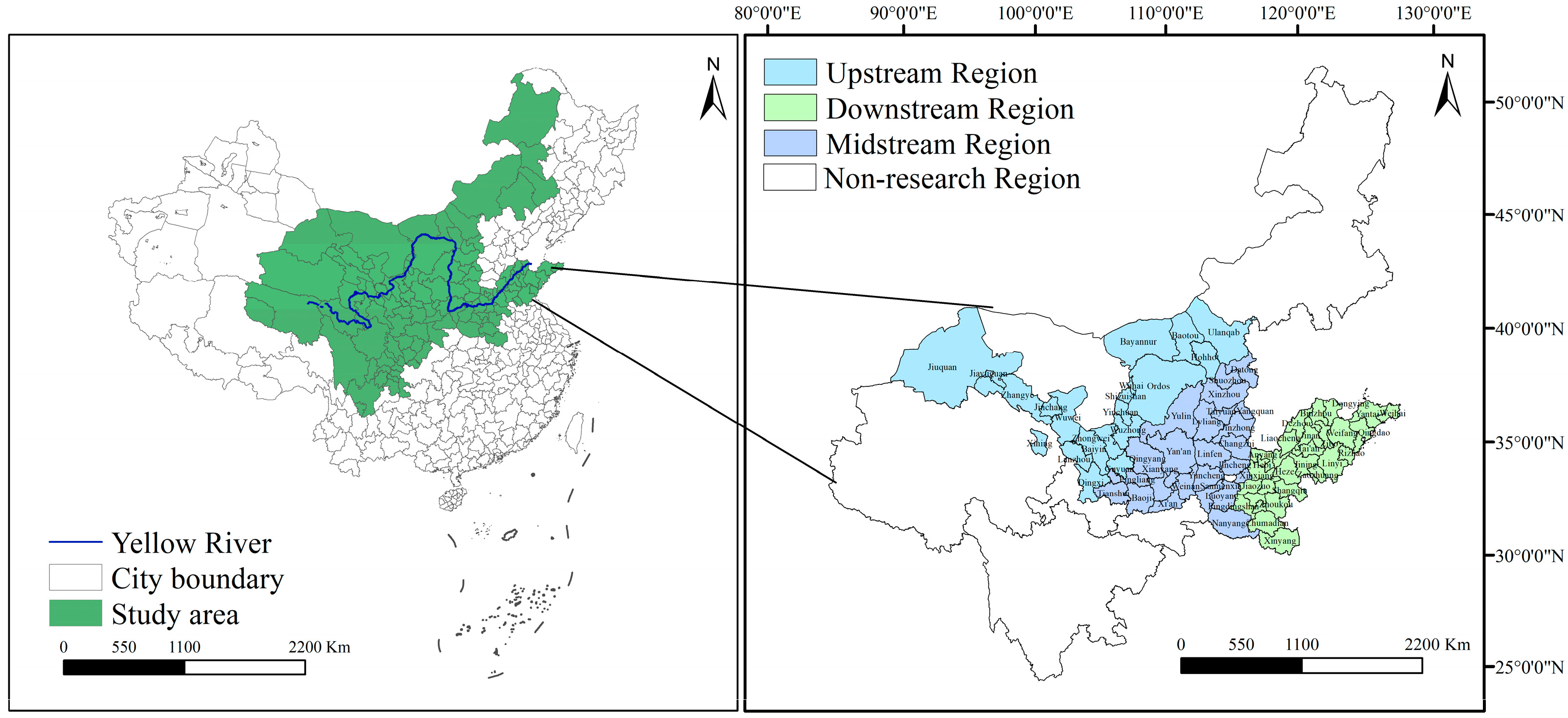
4.1. Study Area

The YRB has a fragile ecosystem. Its economy relies heavily on heavy industry. Economic development in the region is uneven. The YRB is undergoing rapid industrialization and urbanization. These factors make achieving the dual carbon goals both demanding and challenging. Consequently, the YRB is a focal area for advancing the CCD between CEE and CB.

With reference to the 2021 Outline for Ecological Protection and High-Quality Development of the YRB, the river’s main course traverses nine provinces and autonomous regions. We exclude Sichuan Province and eastern Inner Mongolia (the “Mengdong” region) because they fall under other national plans [10]. This study thus focuses on the remaining eight provinces’ prefecture-level cities along the mainstream. For data consistency, we removed cities with missing data or recent administrative changes. The final sample comprises 74 cities. As illustrated in Figure 1, the upstream region encompasses 24 cities. The midstream region includes 23 cities. The downstream region comprises 27 cities.

4.2. System of Indicators

4.2.1. Indicators for CEE

Measurement of CEE depends on clearly defined input and output variables. Following established literature [48] and considering data quality and availability, three inputs were selected for the Super-SBM model: capital stock, number of employees, and energy consumption. Gross domestic product (GDP) and CEs serve as the desired and undesired outputs, respectively (

Table 1. Urban carbon efficiency indicators and calculations.

Primary Indicator	Secondary Indicator	Description
Input Indicators	Labor	Number of employees [7].
	Capital	Capital input is measured by the capital stock [7]. Capital stock is estimated using the Perpetual Inventory Method, employing the following equation, $K_{i,t}=K_{i,t-1}\left(1-{\delta }_{i,t}\right)+I_{i,t}$, where $K_{i,t}$ denotes the capital stock (in CNY 100 million); $\delta$ represents the capital depreciation rate, estimated at 9.6% based on existing research; and $I_{i,t}$ represents capital flow (in CNY 100 million).
	Energy	Referring to existing research, the correlation coefficient between provincial-level data is calculated and applied to city-level data. Nighttime light data at the city level is used to infer city-level energy consumption. ArcGIS is utilized to compute the total DN values for each prefecture-level city in mainland China, from which the simulated energy consumption for each city is estimated and spatialized, ultimately obtaining the total energy consumption data [19].
Desirable Output	GDP	GDP calculated at constant 2006 prices [19,49].
Undesired Output	CEs	CE data sourced from the Center for Global Environmental Research (CGER) [50].

).

4.2.2. Indicators for CB

CB measures the degree to which a region’s carbon sinks and emissions neutralize each other. Typically, CB is expressed as the relationship between CEs and CS. The ecological sustainability coefficient (ESC) equals the ratio of a city’s carbon sink to its CEs [28]. ESC removes intercity differences and effectively represents CB. Data on CEs are based on the emissions dataset available through the Center for Global Environmental Research (CGER). CSs are estimated using land-type specific CS coefficients [51].

4.3. Methods

4.3.1. The Super-SBM Model

Since the SFA method requires the construction of a production function to determine the production frontier, it may result in bias due to incorrect functional form specification [36]. The traditional DEA model is considered objective because it does not require a predefined functional form; however, it fails to account for input-output slack [52]. The SBM model addresses this limitation and can evaluate efficiency, including undesirable outputs, but it cannot differentiate and rank efficient units [53]. The Super-SBM model enables effective comparison and ranking of decision-making units and has been widely applied in the evaluation of ecological and environmental efficiency [54]. In this study, the carbon CEE of the YRB is measured by using MATLAB R2021b. The calculation equation is as follows:

$$\left\{\begin{array}{c}\rho =\min {\displaystyle \frac{1-\frac{1}{N}{\displaystyle \sum _{n=1}^N{s}_n^{x/}}{x}_{kn}^t}{1+\frac{1}{M+1}\left({\displaystyle \sum _{m=1}^M{s}_m^y}/y_{kn}^t+{\displaystyle \sum _{i=1}^t{s}_i^{b/}}{b}_{ki}^t\right)}}\\ \mathrm{s}.\mathrm{t}. {\displaystyle \sum _{t=1}^T{\displaystyle \sum _{k=1}^{K-1}{z}_k^t}}{x}_{kn}^t+s_n^x=x_{kn}^t (n=1,2,\dots ,N)\\ {\displaystyle \sum _{t=1}^T{\displaystyle \sum _{k=1}^{K-1}{z}_k^t}}{y}_{kn}^t-s_m^y=y_{kn}^t (m=1,2,\dots ,M)\\ {\displaystyle \sum _{t=1}^T{\displaystyle \sum _{k=1}^{K-1}{z}_k^t}}{b}_{ki}^t+s_i^b=b_{ki}^t (i=1,2,\dots ,l)\\ z_k^t⩾0,s_n^x⩾0,s_m^y⩾0,s_i^b⩾0\end{array}\right.$$

(1)

where $\rho$ represents the CEE, and $N$, $M$, and $I$ represent the numbers of input, desirable output, and undesirable output indicators, respectively.$x_{kn}^t$, $y_{kn}^t$, and $b_{ki}^t$ denote the n-th input, m-th desirable output, and i-th undesirable output. $z$ is the intensity variable, and $s_n^x$, $s_m^y$, and $s_i^b$ denote the slack variables for inputs, desirable outputs, and undesirable outputs, respectively. The value of $\rho$ lies in (0,1). A DMU is considered efficient if $s_n^x=s_m^y=s_i^b=0$ and $\rho$ = 1; it is inefficient when 0 ≤ $\rho$ < 1.

4.3.2. Carbon Balance Estimation

The carbon sink coefficient method is a commonly used approach for estimating carbon sequestration associated with land use [55]. This method is applicable to land types such as forests, grasslands, water bodies, and unused lands, which serve as primary carbon sinks. The calculation is performed using the following equation:

$$C{S}_{ij}={\displaystyle \sum _n^0\left(A_n\times {\alpha }_n\right)}$$

(2)

where $A_n$ represents the area of land use type n—including forests, grasslands, water bodies, orchards, and unused lands—and ${\alpha }_n$ denotes the carbon sink coefficient (t/hm²) for land type $n$. $C{S}_{ij}$ for region $j$ in year $i$ is calculated as the sum of the products of $A_n$ and ${\alpha }_n$. Following established research practices, cropland is treated as a net carbon source due to its higher emissions from agricultural activities and thus is excluded from the carbon sink calculation (

Table 2. Land types and carbon sink coefficients.

Land Use Type	Carbon Sequestration Coefficient (t/hm2)
Forest Land	0.644
Grassland	0.022
Water Bodies	0.253
Unused Land	0.005

).

Data on CEs utilized in this study were derived from the CGER, which provides 1 km × 1 km resolution gridded datasets. These datasets encompass CEs resulting from fossil fuel combustion, cement production, and natural gas usage. The data were clipped to China’s geographical boundaries and aggregated annually for each city within the YRB from 2006 to 2022.

This study employs the Ecological Support Coefficient (ESC) to assess carbon balance [28]. The ESC is defined as the ratio of a city’s share of CS to its share of CEs within the YRB. This indicator helps eliminate the influence of regional differences and reflects the capacity of local ecosystems to offset total CEs, representing the strength of CB capability. The exact equation is presented below:

$$ESC={\displaystyle \frac{C{S}_{ij}}{{\displaystyle \sum _{ij}C}{S}_{ij}}}/{\displaystyle \frac{C{E}_{ij}}{{\displaystyle \sum _{ij}C}{E}_{ij}}}$$

(3)

where $CS$ and $CE$ represent the total carbon sink and carbon emissions in the YRB, respectively; $i$ denotes the year; and $j$ indicates the city. When the ESC exceeds 1, it signifies a strong carbon sink capacity and a favorable carbon balance. Conversely, an ESC below 1 reflects a weaker carbon balance capacity.

4.3.3. The Coupling Coordination Model

The concept of coupling degree, originating from physics, quantifies the interaction between subsystems within a complex system. Building upon this, the coupling coordination degree (CCD) model assesses both the strength of these interactions and the harmony of subsystem developments. In this study, all data were first standardized. Drawing from existing literature [56], the CCD model is calculated as:

$$C={\displaystyle \frac{2\sqrt{U_1{U}_2}}{U_1+U_2}}$$

(4)

$$D=\sqrt{C\times T}, T=\alpha U_1+\beta U_2$$

(5)

where $C$ represents the coupling degree; $U_1$ and $U_2$ denote the normalized CEE and CB, respectively; and $T$ serves as an integrated index reflecting the overall level of coordination of CEE and CB. $\alpha$ and $\beta$ are undetermined coefficients set to 0.5 to give equal weight to CEE and CB. $D$ reflects the coupling coordination degree. The variable spans the closed unit interval (0,1) with higher values signifying stronger coordination. Based on existing studies [57], $D$ is classified into five categories: severe imbalance (0 < $D$ < 0.2), moderate imbalance (0.2 < $D$ < 0.4), antagonism (0.4 < $D$ < 0.6), moderate coordination (0.6 < $D$ < 0.8), and high coordination (0.8 < $D$ < 1).

4.3.4. The Kernel Density Estimation

Kernel density estimation applies a smooth kernel function to sample data to generate a continuous density curve that depicts the distribution of a random variable [58]. In this study, kernel density estimation with a Gaussian kernel is applied to estimate the probability density of the CCD. Continuous density curves then visualize its dynamics. This study conducts visualization analysis using MATLAB R2021b. Let $x$ be a random variable with density function:

$$f(x)={\displaystyle \frac{1}{Nh}}{\displaystyle \sum _{i=1}^{N}K}\left({\displaystyle \frac{x_i-\overline{x}}{h}}\right)$$

(6)

where $x_i$ is independent and identically distributed observations, $\overline{x}$ stands for the mean, $N$ is the number of observations, $h$ is the bandwidth, and $K(.)$ is the kernel function.

4.3.5. The Spatial Autocorrelation Analysis

Spatial autocorrelation analysis is a method of statistical analysis that assesses the degree to which similar or dissimilar values cluster together across geographic space, revealing patterns of spatial dependence such as clustering or dispersion [59]. Moran’s I is a commonly employed metric for evaluating spatial autocorrelation. It evaluates whether the values of a variable in neighboring spatial units are more similar (indicating clustering) or dissimilar (indicating dispersion) than would be expected under spatial randomness. In this study, Moran’s I index is employed to assess the spatial autocorrelation of the CCD across the YRB, providing insights into the spatial distribution patterns of CCD in the region. This study uses ArcGIS 10.8 software to visualize spatial autocorrelation levels. The equation is as follows:

$$\begin{array}{l}I={\displaystyle \frac{n{\displaystyle \sum _{i=1}^n{\displaystyle \sum _{j=1}^n{W}_{ij}}}\left(X_i-\overline{X}\right)\left(X_j-\overline{X}\right)}{{\displaystyle \sum _{i=1}^n{\displaystyle \sum _{j=1}^n{W}_{ij}}}{\displaystyle \sum _{i=1}^n{\left(X_i-\overline{X}\right)}^2}}}\\ I_i={\displaystyle \frac{n\left(X_i-\overline{X}\right)}{{\displaystyle \sum _{i=1}^n{\left(X_i-\overline{X}\right)}^2}}}{\displaystyle \sum _{j=1,j\ne i}^n{W}_{ij}}\left(X_j-\overline{X}\right)\end{array}$$

(7)

where $I$ and $I_i$ represent the global and local Moran’s I index, respectively, assessing spatial dependencies at regional and local scales; $N$ denotes the number of cities in the YRB; $X$ denotes CCD; and $Wij$ is the spatial weight matrix, constructed using the commonly applied geographic distance matrix:

$$W_{ij}=\left\{\begin{array}{l}{\displaystyle \frac{1}{d_{ij}}},i\ne j\hfill \\ 0,i=j\hfill \end{array}\right.$$

(8)

where d_ij denotes the straight-line geographical distance between cities $i$ and $j$.

4.3.6. Dagum Gini Coefficient and Its Decomposition

The Gini coefficient decomposition method proposed by Dagum addresses the inherent indivisibility limitation of the traditional Gini index and has been extensively employed in the analysis of regional disparities and inequalities [60]. The Dagum Gini coefficient and its decomposition approach are utilized in this study to analyze spatial variations in the CCD across the YRB. According to Dagum’s decomposition framework [58], the overall inequality ($G$) can be partitioned into three components: intra-regional disparity ($G_w$), inter-regional disparity ($G_{nb}$), and transvariation intensity ($G_t$), satisfying the relation $G$=$G_w$=$G_{nb}$=$G_t$. The specific calculation equation is as follows:

$$G={\displaystyle \sum _{j=1}^k{\displaystyle \sum _{h=1}^k{\displaystyle \sum _{i=1}^{n_j}{\displaystyle \sum _{r=1}^{n_h}\left|y_{ji}-y_{hr}\right|}}}}/2n^2\overline{y}$$

(9)

where $y$ denotes CCD; $y_{ji}(y_{hr})$ represents the coordination level of any city within region $j(h)$; $n$ is the total number of cities; $k$ indicates the number of regions; and $n_j(n_h)$ is the number of cities within region $j(h)$.

4.3.7. Markov Chain Analysis

This study also employs the Markov chain approach to capture the dynamic evolution of regional development [61]. The Markov process treats regional changes as transitions between discrete states over time, allowing an assessment of each city’s status and its likelihood of upward or downward movement. The state transition equation is as follows:

$$P_{ij}={\displaystyle \frac{z_{ij}}{z_i}}$$

(10)

where $P_{ij}$ represents the probability that the CCD is associated with type $i$ at moment $t$ and type $j$ at moment $t+1$; $z_{ij}$ represents the total count of cities whose CCD level is associated with type $i$ at moment $t$ and type $j$ at moment $t+1$; and $z$ represents the total count of cities whose CCD level is associated with type $i$.

$$\mathrm{Spatial} \mathrm{lag} \mathrm{values}, La{g}_a={\displaystyle \sum _{b=1}^n{W}_{ab}}{Y}_b$$

(11)

where $La{g}_a$ represents the spatial $lag$ value of region $a$, and $n$ represents the total quantity of cities. The spatial weight matrix $W_{ab}$ represents the spatial adjacent relationship between region $a$ and region $b$. The adjacent principle is used to define spatial relationships in this study, and $Y_b$ represents the observed value of region $b$.

4.3.8. The Extreme Gradient Boosting (XGBoost) Algorithm

XGBoost, a machine learning approach, is rooted in the gradient boosting decision tree (GBDT) model. It constructs a series of weak learners, each addressing the residuals of the previous model. This sequential fitting boosts overall prediction accuracy [62]. On high-dimensional or complex tasks, XGBoost delivers superior precision with lower computational cost. It also mitigates overfitting effectively. These features underpin XGBoost’s widespread use in regression analysis. The objective function of XGBoost is defined as follows:

$$\mathrm{Objective} ={\displaystyle \sum _{i=1}^n\mathrm{loss}}\left(y_i,{\widehat{y}}_i\right)+{\displaystyle \sum _{k=1}^k\mathrm{\Omega }}\left(f_k\right)$$

(12)

where $\mathrm{loss}\left(y_i,{\widehat{y}}_i\right)$ is the loss function, measuring the discrepancy between predicted and actual values, and $\mathrm{\Omega }\left(f_k\right)$ is the model’s regularization term, used to control model complexity and prevent overfitting.

4.3.9. The SHAP Value Explanation Algorithm

The SHAP value algorithm provides an effective way to explain machine learning predictions. The method is grounded in the Shapley value concept from cooperative game theory [63]. It quantifies each feature’s contribution and direction of effect on CEE and CB. This study performs visualization using Python 3.9.13. Let the feature set be $\left\{x_1,x_2,\dots ,x_p\right\}$. Let $S$ be any subset of features not containing $x_i$, and let $\left|S\right|$ be its size. Let $f(S)$ denote the model output for the feature subset $S$. Let $f(S\cup \left\{x_i\right\})$ denote the output after adding $x_i$ to $S$. Thus, the SHAP value for $x_i$ is computed as:

$$\mathrm{SHAP}\left(x_i\right)={\sum }_{S\subseteq \left\{x_1,x_2,\dots ,x_p\right\}\backslash \left\{x_i\right\}}{\displaystyle \frac{\left|S\right|!(p-|S|-1)!}{p!}}\left[f\left(S\cup \left\{x_i\right\}\right)-f(S)\right]$$

(13)

Thus, SHAP values consider every possible feature subset and compute the weighted average of the change in model output before and after adding feature $x_i$. This process determines feature $x_i$’s contribution to the target. The SHAP explanation method accurately identifies the key features and supports more efficient, more precise decision making.

4.4. Data Sources and Processing

This study integrates data from multiple authoritative sources to ensure analytical accuracy and spatial resolution. Statistical data—including fixed asset investment, GDP, science and education inputs, employment, fiscal expenditure, population, industrial enterprises above a designated size, total retail sales of consumer goods, and electricity consumption—are primarily sourced from the China City Statistical Yearbook and the National Bulletin of Science and Technology Investment Statistics, with missing values imputed using the moving average method. Energy data are drawn from the China Energy Statistical Yearbook. Land use data were obtained from the China Land Cover Dataset (CLCD) (https://zenodo.org/records/8176941) (accessed on 1 April 2025), which is derived from 30-meter multispectral imagery under the WGS-84 coordinate system. In this study, the data were reclassified into seven land use types: cropland, forest Land, grassland, water bodies, wetlands, built-up land, and unused land. Following preprocessing to remove noise and correct classification errors, zonal statistics in ArcGIS 10.8 were applied to calculate land use areas at the prefecture-level city scale. Missing values were addressed using multiple imputations.Carbon emissions (CEs) data are derived from the 1 km × 1 km gridded ODIAC database developed by CGER, NIES, Japan (https://db.cger.nies.go.jp/dataset/ODIAC/data_policy.html) (accessed on 1 April 2025), and were reprojected and masked in ArcGIS 10.8 to extract regional emissions data for China. Nighttime light data are from the enhanced DMSP-OLS-like dataset (https://dataverse.harvard.edu/dataset.xhtml?persistentId=doi:10.7910/DVN/GIYGJU) (accessed on 1 April 2025), with a 1 km × 1 km resolution and strong correlation with energy consumption (R² = 0.931 nationally, 0.65 provincially). A linear simulation model was used to estimate and spatialize energy consumption for 74 cities in the YRB based on grayscale values processed in ArcGIS. Precipitation data are provided by the U.S. NCEI (https://www.ncei.noaa.gov/) (accessed on 1 April 2025), offering high spatial and temporal accuracy, while temperature data are from the China Daily Surface Climate Data Set V3.0 by the China Meteorological Data Service Center (http://data.cma.cn/) (accessed on 1 April 2025), which has undergone strict quality control and standardization.

5. Results

5.1. Spatiotemporal Evolution of CEE and CB

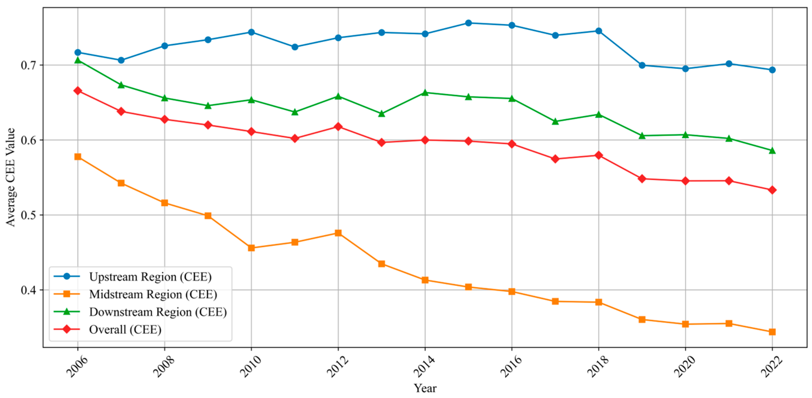
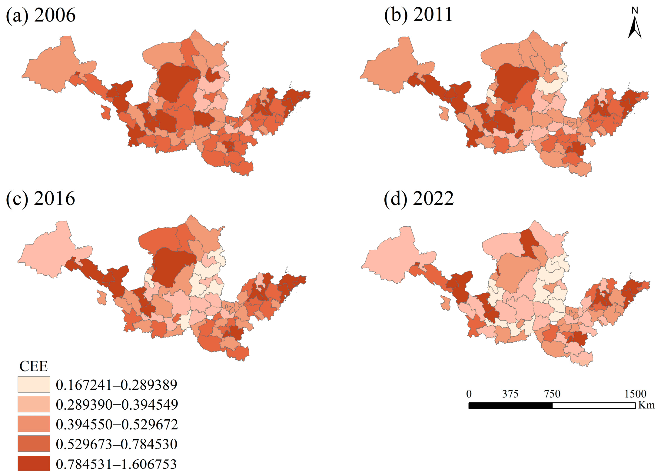
5.1.1. Spatiotemporal Evolution of CEE

As shown in Figure 2, the average CEE was 0.59, indicating a relatively low efficiency level. From 2006 to 2022, CEE declined from 0.67 to 0.53, with an average annual decrease of 1.45%. Regionally, the upstream region saw a slight decline from 0.72 to 0.69, decreasing by 0.21% annually. The downstream region dropped from 0.71 to 0.59, with an annual decrease of 1.16%. The midstream region experienced a sharp fall from 0.58 to 0.34, decreasing by 3.19% per year. The downward trend since 2019 may be linked to economic stagnation caused by the COVID-19 pandemic. Periodic increases in CEE occurred in 2011–2012 and 2017–2018, likely driven by national policies such as the Twelfth Five-Year Plan launched in 2011, which targeted energy efficiency in high-consumption industries, and the Thirteenth Five-Year Plan for greenhouse gas emission control introduced in 2016, which implemented stricter energy and emission targets. However, between 2012 and 2016, policy effects diminished while energy-intensive industries expanded, leading to a decline in CEE. After 2018, despite more technology upgrade projects being approved, many small and medium-sized cities faced funding shortages, a lack of technical personnel, and limited equipment, which restricted further improvement in CEE. Figure 3 shows that high CEE levels are mainly concentrated in the upstream and downstream regions, while the midstream region has relatively lower efficiency. In 2006, 17 cities including Dongying, Zhongwei, and Linfen led in CEE, accounting for 22.97% of the total, but by 2022, this number dropped to 11 cities such as Zhongwei, Wuhai, and Baotou, representing 14.86%. Throughout the period, cities like Jinchang and Jiayuguan consistently maintained high CEE, whereas resource-dependent cities such as Xinzhou and Yinchuan exhibited lower efficiency. Cities including Baotou, Jinan, and Jiayuguan showed significant CEE improvements, reflecting successful carbon reduction efforts, while Jining, Kaifeng, and Ordos experienced declines amid increasing carbon reduction pressures. Some cities including Dongying, Tai’an, and Weihai showed fluctuating CEE levels. High-CEE cities fall into three types: those achieving industrial upgrading through advanced manufacturing and modern services, such as Jinan, Qingdao, and Yantai; those developing low-carbon production by leveraging abundant natural or renewable resources and clean technologies, like Jiayuguan, Jinchang, Wuwei, and Guyuan; and those promoting industrial transformation via targeted green fiscal subsidies and strict environmental enforcement, including Zibo, Baotou, Wuhai, and Qingdao. In contrast, low-CEE cities face diverse challenges. Some, such as Linyi, Rizhao, Jiaozuo, and Liaocheng, remain reliant on labor-intensive, high-energy industries, limiting efficiency gains. Others, including Ulanqab, Yulin, Ordos, and Zhangye, confront transition difficulties due to resource depletion or ecological constraints. Additionally, cities like Zhengzhou, Xi’an, and Taiyuan lack sufficient policy incentives and effective implementation, resulting in weak motivation for low-carbon transformation.

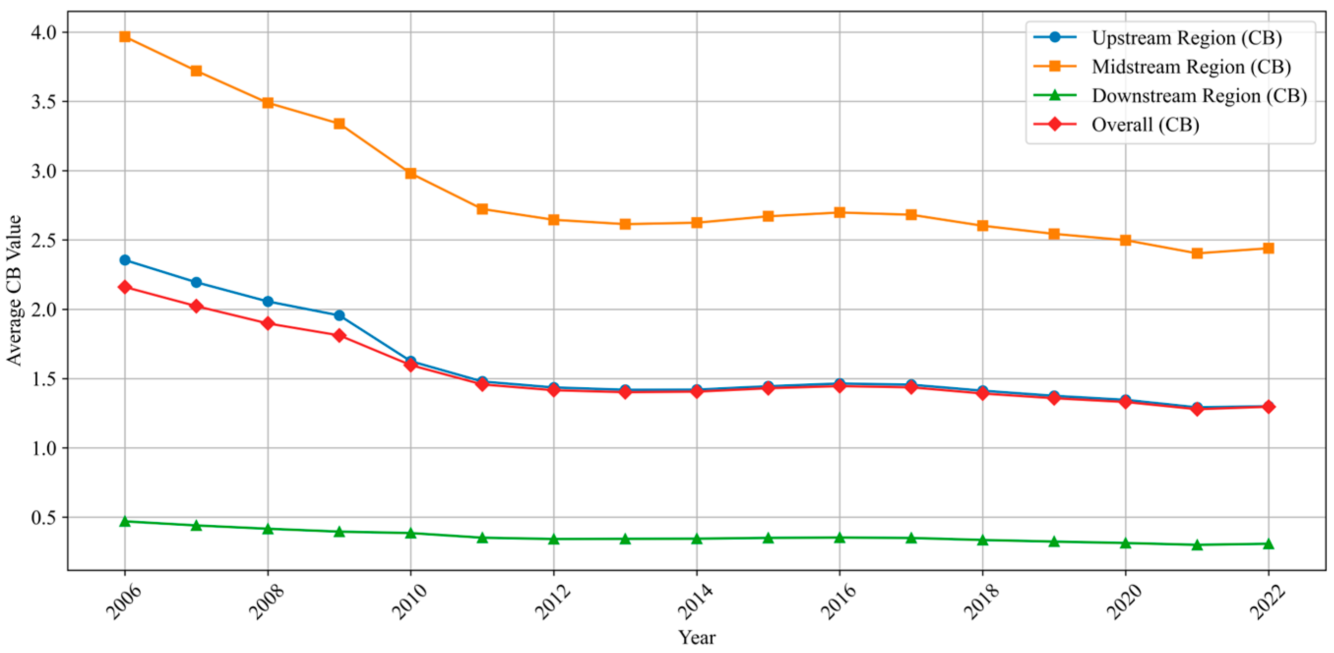
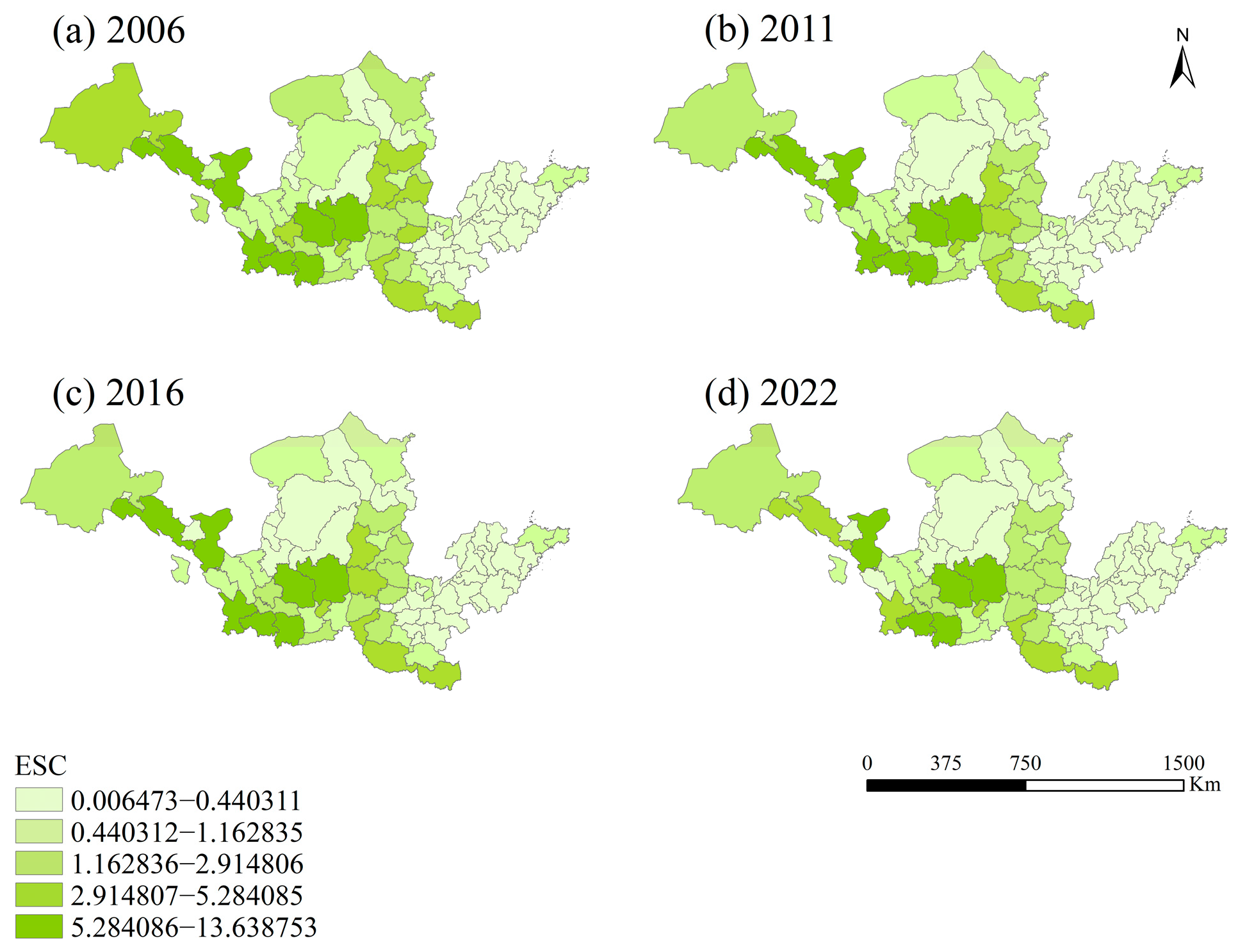
5.1.2. Spatiotemporal Evolution of CB

As shown in Figure 4, the temporal trend of CB exhibits a general decline, dropping from 2.16 in 2006 to 1.30 in 2022, with an average annual decrease of 3.14%. Although slight increases occurred in 2015 and 2016, the overall downward trend persisted. Regionally, the midstream CB decreased from 3.97 to 2.44 at an annual rate of 2.99%, the upstream region declined from 2.36 to 1.30 at 3.64% per year, and the downstream region fell from 0.47 to 0.31 at 2.60% annually. The rapid decline in CB from 2006 to 2012 in the YRB and its upstream and midstream regions coincides with the expansion of resource-intensive industries and heavy energy consumption, particularly in the midstream and upstream areas, which intensified carbon emissions and imbalance. After 2012, the implementation of policies such as the National Main Functional Area Planning and ecological protection red lines tightened land-use controls, increased ecological land, and slowed construction land expansion, thereby enhancing carbon sequestration and stabilizing CB decline. The downstream region maintained a stable low CB throughout, likely due to its dense population and high urbanization, where concentrated industrial and daily energy demands create rigid carbon emissions, keeping CB consistently low. Figure 5 shows that CB levels are relatively high in the upstream and midstream regions, while the downstream region has a comparatively lower CB. During the study period, only Dongying and Binzhou experienced slight CB increases, whereas most cities saw declines. By 2022, 24 cities achieved positive CB, 7 fewer than in 2006. Spatial heterogeneity in CB across cities is influenced by ecological conditions, industrial structure, and policy orientation. Cities with a CB above 1, such as Yan’an, Lüliang, and Qingyang, are mainly located in the Loess Plateau and ecological restoration zones in Northwest China, where large-scale programs like Grain for Green and the Three North Shelterbelt have enhanced carbon sinks. Low industrialization levels further limit emissions, supporting net positive CB. Similarly, Central Plains cities like Xinyang, Nanyang, and Zhumadian exhibit a CB above 1 due to agriculture-based economies and favorable ecological endowments. In contrast, cities such as Taiyuan, Baotou, and Lanzhou, dominated by energy-intensive industries and coal-based energy mixes, have high emissions and limited carbon sinks, resulting in a CB below 1. Highly industrialized metropolitan areas like Qingdao, Zhengzhou, and Jinan also show a relatively low CB despite some ecological capacity due to concentrated emissions from urban and industrial activities. Variations in CB among some cities suggest internal disparities or instability in local carbon dynamics.

5.2. The Spatiotemporal Evolution of CCD

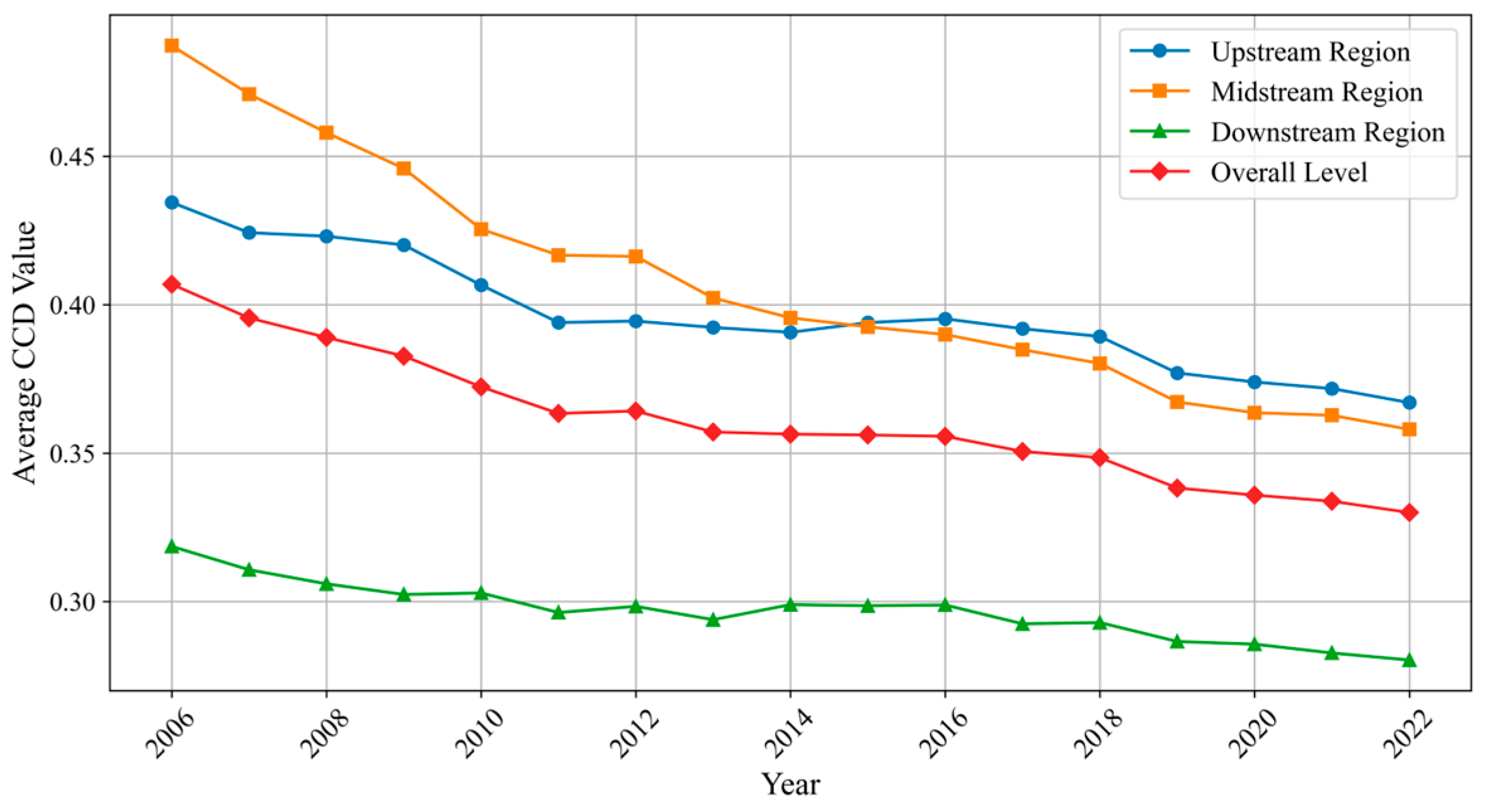
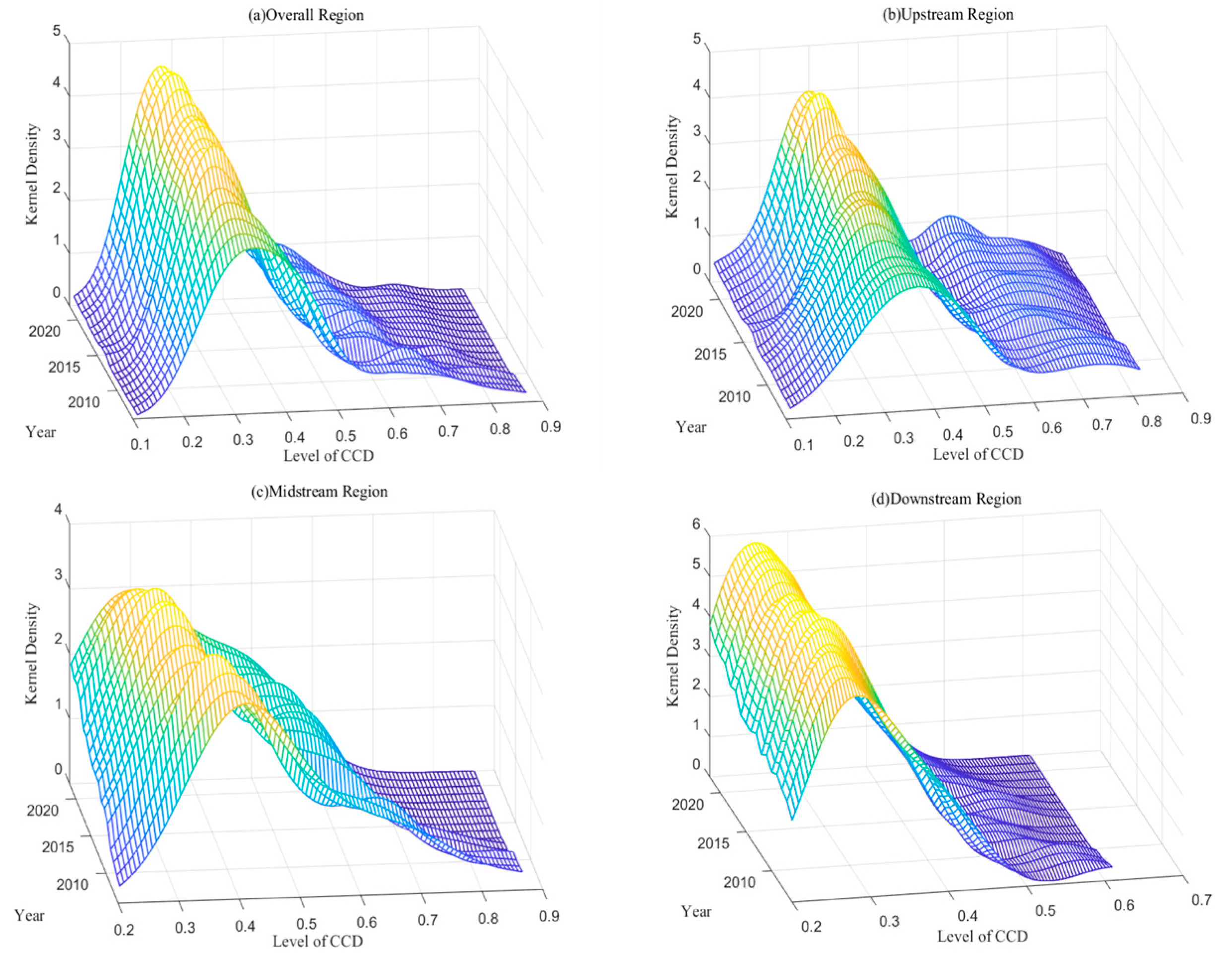
5.2.1. The Temporal Evolution of CCD

As illustrated in Figure 6, the CCD between CEE and CB exhibited a fluctuating downward trend, with a mean value of 0.36, indicating a generally low degree of CCD. The CCD declined from 0.41 in 2006 to 0.33 in 2022, with an average annual decrease of approximately 1.30%. In the midstream region, CCD decreased from 0.49 to 0.36 at an average annual rate of 1.91%, remaining higher than the overall YRB average. The upstream region showed a decline from 0.43 to 0.37, with an annual average decline of 1.05%, also above the basin average. The downstream region experienced the lowest coordination level, dropping from 0.32 to 0.28, with an annual decrease of 0.80%. Both the upstream and downstream regions exhibited a pattern of initial decline, subsequent recovery, and then another decline. Overall, from 2006 to 2015, the CCD ranking followed midstream > upstream > downstream, whereas from 2016 to 2022, the order shifted to upstream > midstream > downstream. Corresponding to the gradual decline in CCD, the overall coupling coordination level moved from the “Antagonism” stage in 2006 into the “Moderate Imbalance” stage. Regionally, the upstream and midstream regions transitioned from “Antagonism” to “Moderate Imbalance” in 2013 and 2014, respectively, while the downstream region remained in the “Moderate Imbalance” stage throughout the study period. The coordination status in the upstream and midstream regions was generally better than in the downstream region.

Kernel density estimation (KDE) was applied to assess temporal variations in the CCD. As shown in Figure 7a,d, the distribution curve shifts leftward over time, indicating a gradual reduction in CCD. The main peak height increases while the curve narrows slightly, suggesting that regional coordination levels are converging, and absolute differences are shrinking. A pronounced right tail appears, revealing that a few cities significantly outperform others and that the absolute gap continues to widen. Bimodal or multimodal patterns emerge at the basin level, indicating polarization; secondary peaks shift leftward, implying that leading regions’ performance is weakening.

Throughout the upstream and midstream regions, the curves in Figure 7b,c shift leftward, showing region-level declines consistent with the basin trend. In the upstream region, the main peak height increases, and the curve widens, suggesting convergence of coordination levels. However, absolute differences among upstream cities continue to expand, as evidenced by the presence of several secondary peaks adjacent to the primary peak. In the midstream region, the main peak exhibits an “M”-shaped trajectory, characterized by alternating phases of increase and decrease, accompanied by a gradual narrowing of the curve, and absolute differences shrink. Recently, midstream curves have shown varying degrees of bimodality, first rising then falling, indicating a weakening of CCD polarization. A clear right tail persists, reflecting significant disparities in city-level CCD within these regions.

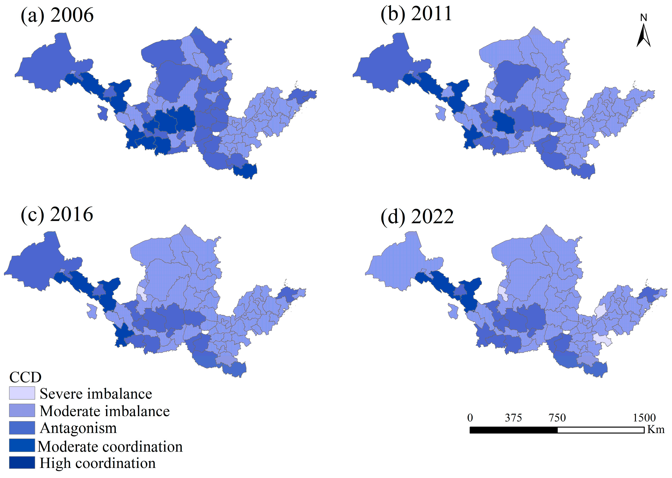
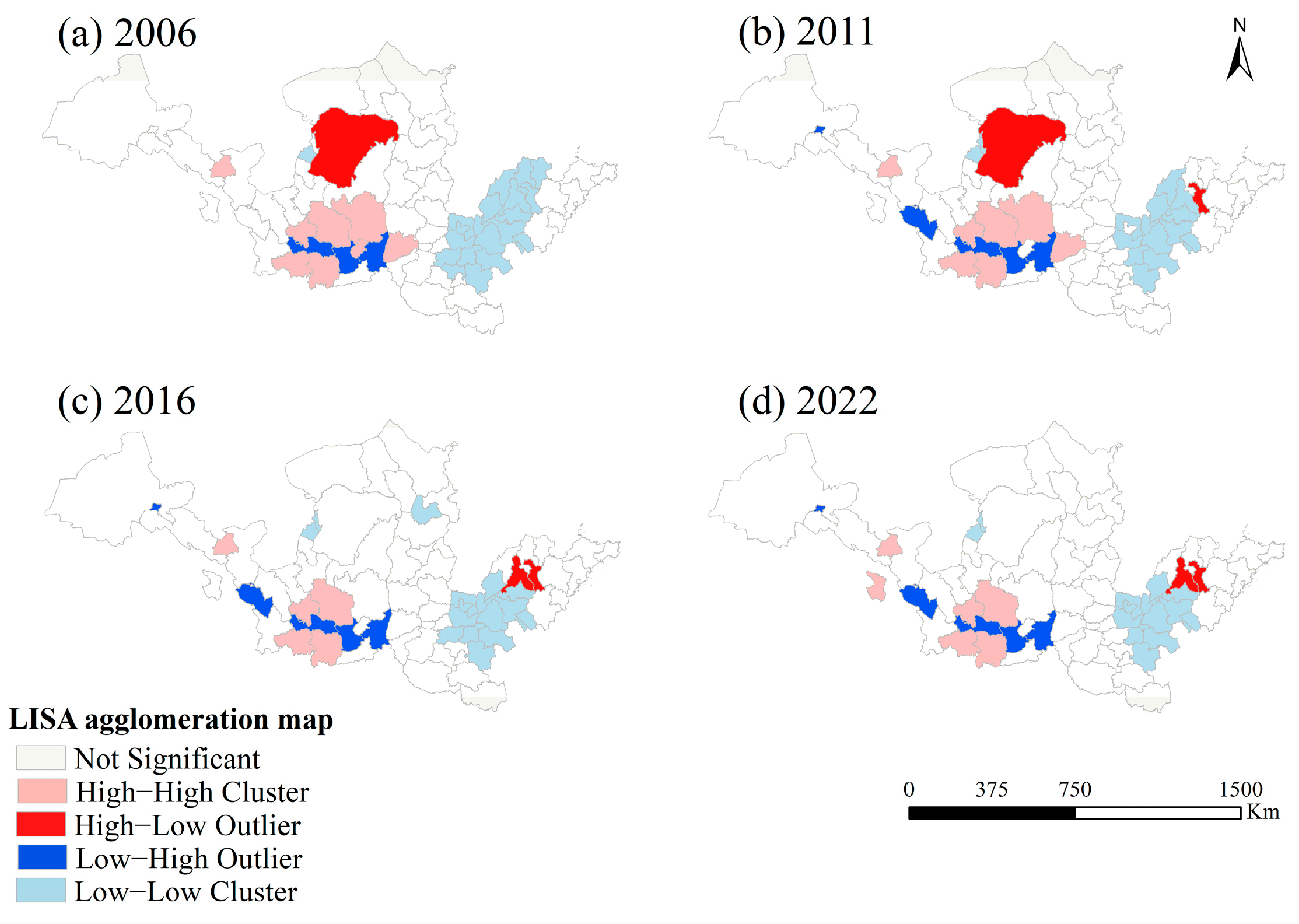
5.2.2. Spatial Distribution Characteristics of the CCD

To analyze the spatial heterogeneity of CCD across the YRB, we selected four time slices: 2006, 2011, 2016, and 2022. Spatial visualization was performed using ArcGIS 10.8. Figure 8 shows a low-east, high-west pattern, with CCD decreasing from west to east. Over the study period, the spatial distribution of CCD changed markedly and declined overall. Cities with a high CCD clustered in the upstream and midstream regions, forming a clustered distribution. Downstream cities maintained a moderate imbalance and showed no sign of improvement. From the city perspective, from 2006 to 2022, overall CCD trended downward. The number of cities in imbalance grew, while those in coordination declined. Yinchuan became the first city to enter severe imbalance. No city achieved high coordination during this period. By 2022, 16 cities had a CCD of antagonism or above, representing 21.62% of all cities surveyed. Most cities remained in moderate imbalance, mainly in midstream and downstream regions. Shangqiu, Liaocheng, and Yinchuan were in severe imbalance.

5.2.3. Spatial Autocorrelation of the CCD

Utilizing an adjacency-based spatial weight matrix, the global Moran’s I index was calculated to assess the spatial autocorrelation of CCD between CEE and CB during the period from 2006 to 2022. The findings, shown in

Table 3. Global Moran’s I index.

Year	Global Moran’s I	Z-Values	p-Values
2006	0.361	4.734	0.000
2007	0.353	4.627	0.000
2008	0.346	4.556	0.000
2009	0.331	4.366	0.000
2010	0.327	4.302	0.000
2011	0.324	4.274	0.000
2012	0.322	4.245	0.000
2013	0.331	4.349	0.000
2014	0.349	4.578	0.000
2015	0.347	4.557	0.000
2016	0.341	4.491	0.000
2017	0.336	4.426	0.000
2018	0.334	4.401	0.000
2019	0.359	4.729	0.000
2020	0.356	4.690	0.000
2021	0.352	4.645	0.000
2022	0.345	4.552	0.000

, indicate that Moran’s I decreased from 0.361 in 2000 to 0.345 in 2022, suggesting a declining trend in spatial clustering of similar CCD levels among cities. Despite this decline, the Z-values exceeded 2.58 in all cases, and the p-values were consistently below 0.01, confirming statistical significance at the 99% confidence level. These findings demonstrate a persistent, though slightly diminishing, positive spatial autocorrelation in CCD across the YRB. Spatially, the CCD exhibited distinct high-high and low-low clustering patterns, indicating that cities with similar coordination levels tend to be geographically proximate.

As shown in Figure 9, the local spatial autocorrelation analysis indicates notable clustering patterns in the CCD throughout the YRB, with high-high clusters mainly found in the midstream and parts of the upstream regions. These areas have likely implemented proactive measures such as optimizing energy structures, promoting clean energy adoption, and advancing ecological restoration efforts, collectively contributing to enhanced CCD levels. Conversely, low-low clusters are mainly situated in the downstream regions, particularly in Henan and Shandong provinces. The dominance of traditional heavy industries in these regions—marked by high energy intensity, elevated carbon emissions, and limited energy diversification—has contributed to persistently low CCD levels. The high-high clusters remained relatively stable over time but did not effectively generate spatial spillover effects to neighboring areas. In contrast, the number of low-low cities increased from 20 in 2006 to 31 in 2022, indicating a growing convergence effect among these regions. This trend suggests that downstream cities lack robust inter-city cooperation mechanisms and cross-regional linkages. Therefore, strengthening collaboration among regions and cities is crucial for improving CCD in the downstream regions of the YRB.

5.2.4. Spatial Disparities of the CCD

Table 4. Dagum Gini coefficient and contribution rate results.

Year	Gini Coefficient				Rate of Contribution (%)
	G	Gw	Gnb	Gt	Gw	Gnb	Gt
2006	0.197	0.054	0.097	0.046	27.478	49.193	23.330
2007	0.197	0.055	0.095	0.048	27.687	48.072	24.241
2008	0.195	0.054	0.092	0.049	27.687	47.178	25.136
2009	0.197	0.055	0.088	0.053	28.119	44.841	27.039
2010	0.186	0.053	0.078	0.056	28.382	41.680	29.938
2011	0.185	0.053	0.078	0.054	28.602	42.097	29.301
2012	0.184	0.053	0.076	0.054	28.848	41.505	29.647
2013	0.180	0.052	0.072	0.056	28.742	40.022	31.236
2014	0.181	0.053	0.064	0.064	29.195	35.617	35.188
2015	0.181	0.053	0.064	0.064	29.328	35.177	35.495
2016	0.180	0.053	0.064	0.063	29.520	35.557	34.923
2017	0.181	0.053	0.067	0.061	29.340	36.948	33.712
2018	0.178	0.053	0.065	0.061	29.477	36.402	34.121
2019	0.181	0.054	0.063	0.065	29.685	34.605	35.710
2020	0.181	0.054	0.061	0.065	29.861	33.972	36.167
2021	0.179	0.053	0.062	0.063	29.644	34.985	35.370
2022	0.181	0.054	0.062	0.065	29.796	34.056	36.147
Average	0.185	0.053	0.073	0.058	28.907	39.524	31.571

shows that the Gini coefficient reflecting the CCD experienced alternating phases of widening and narrowing from 2006 to 2022, with an overall downward trend. The average Gini coefficient during this period was 0.185. From 2006 to 2011, the coefficient remained above average, indicating relatively high disparities, while from 2012 to 2022, it fell below the average, suggesting a gradual narrowing. Specifically, the coefficient declined from 0.197 in 2006 to 0.181 in 2022, with an average annual reduction of 0.53%. The decomposition results indicate that inter-regional differences contributed the most to overall disparities, followed by super-variable density, with intra-regional differences contributing the least. This reflects an unbalanced pattern of CCD development, with midstream and upstream regions outperforming the downstream region. Over time, the contribution of inter-regional disparities decreased, while intra-regional disparities increased. The rising super-variable density suggests overlapping coordination levels between high- and low-performing regions, indicating increasing complexity in CCD disparities across the YRB.

Table 5. Dagum Gini coefficient difference decomposition results.

Year	Differences Within the Region			Differences Between Regions
	Up	Down	Mid	Up Down	Up Mid	Down Mid
2006	0.209	0.136	0.158	0.217	0.192	0.231
2007	0.211	0.134	0.161	0.218	0.194	0.228
2008	0.210	0.129	0.160	0.219	0.192	0.222
2009	0.213	0.129	0.171	0.221	0.196	0.220
2010	0.215	0.124	0.156	0.211	0.192	0.200
2011	0.210	0.119	0.165	0.204	0.192	0.201
2012	0.206	0.116	0.169	0.200	0.192	0.198
2013	0.203	0.118	0.159	0.201	0.186	0.192
2014	0.215	0.123	0.156	0.206	0.191	0.183
2015	0.211	0.124	0.160	0.207	0.190	0.183
2016	0.205	0.125	0.163	0.203	0.189	0.183
2017	0.207	0.126	0.159	0.206	0.188	0.183
2018	0.204	0.125	0.159	0.203	0.187	0.179
2019	0.211	0.126	0.162	0.204	0.193	0.179
2020	0.213	0.123	0.166	0.202	0.195	0.178
2021	0.21	0.122	0.161	0.202	0.192	0.177
2022	0.211	0.124	0.166	0.203	0.194	0.179
Average	0.210	0.125	0.162	0.207	0.191	0.195

presents the intra- and inter-regional Gini coefficients for the upstream, midstream, and downstream regions of the YRB. In terms of intra-regional variations, the midstream and downstream regions consistently maintained Gini coefficients below the national average, indicating relatively lower internal disparities. In contrast, the upstream region exhibited higher Gini coefficients, reflecting greater internal imbalances. From 2006 to 2022, the Gini coefficient in the upstream region rose slightly from 0.209 to 0.211, with an average annual increase of 0.06%. The midstream region saw a decline from 0.136 to 0.124, averaging an annual decrease of 0.58%, while the downstream region experienced a rise from 0.158 to 0.166, with an average annual increase of 0.31%. These changes suggest that intra-regional disparities narrowed in the midstream region but expanded in the upstream and downstream regions. Regarding inter-regional trends, the Gini coefficients among the three regions were consistently above the national average, indicating pronounced disparities. Among them, the disparity between the upstream and midstream regions was the smallest. From 2006 to 2022, the upstream–downstream disparity declined at an average annual rate of 0.42%, the downstream–midstream disparity decreased by 3.57% annually, while the upstream–midstream disparity increased slightly by 0.03% per year. These results reflect a narrowing trend in disparities between the downstream and other regions, while the upstream–midstream gap slightly widened.

5.2.5. Markov Chain Analysis of CCD

This study categorizes CCD development between CEE and CB into four tiers using a quartile-based classification: low (I), lower-middle (II), upper-middle (III), and high (IV). The Markov transition probability matrix is shown in

Table 6. Traditional Markov transfer probability matrix of CCD.

t/(t + 1)	I	II	III	IV	N
I	0.9828	0.0172	0.0000	0.0000	290
II	0.0614	0.9249	0.0137	0.0000	293
III	0.0000	0.0795	0.9139	0.0066	302
IV	0.0000	0.0000	0.0602	0.9398	299

. The diagonal probabilities exceed 90%, indicating strong state persistence and suggesting conditional convergence at both low and high coordination levels. The probability of cities achieving leapfrog development is minimal; notably, there is a 0% probability of a direct transition from low to high coordination, and only a 0.66% probability of moving from lower-middle to upper-middle coordination. These findings imply that despite ongoing industrialization and urbanization, cities in the YRB continue to depend significantly on high-carbon energy sources. The entrenched high-carbon development model exhibits significant path dependence, making short-term transitions challenging and hindering substantial improvements in CEE and CB levels. The presence of non-zero elements adjacent to the diagonal implies that changes in coupling coordination occur predominantly between neighboring levels. This pattern reflects the gradual nature of CCD development, indicating that substantial leaps in coordination are challenging to realize.

Table 7. Spatial Markov transfer probability matrix of CCD.

Domain Type	t/t + 1	I	II	III	IV	N
I	I	1.0000	0.0000	0.0000	0.0000	118
	II	0.0417	0.9583	0.0000	0.0000	24
	III	0.0000	0.1111	0.8889	0.0000	18
	IV	0.0000	0.0000	0.0000	0.0000	0
II	I	0.9692	0.0308	0.0000	0.0000	130
	II	0.0855	0.8889	0.0256	0.0000	117
	III	0.0000	0.0575	0.9425	0.0000	87
	IV	0.0000	0.0000	0.1667	0.8333	6
III	I	0.9730	0.0270	0.0000	0.0000	37
	II	0.0513	0.9359	0.0128	0.0000	78
	III	0.0000	0.0853	0.9147	0.0000	129
	IV	0.0000	0.0000	0.0734	0.9266	109
IV	I	1.0000	0.0000	0.0000	0.0000	5
	II	0.0405	0.9595	0.0000	0.0000	74
	III	0.0000	0.0882	0.8824	0.0294	68
	IV	0.0000	0.0000	0.0489	0.9511	184

incorporates spatial lag effects into the Markov analysis. Firstly, diagonal probabilities remain significantly higher than off-diagonal ones across different classifications, reinforcing the stability of CCD levels when spatial factors are considered. Secondly, the CCD of a city is affected by the coordination levels of its adjacent cities, demonstrating a spatial clustering effect. Cities with lower CCD levels are more likely to be surrounded by similarly low-performing cities, indicating that spatial distribution patterns significantly impact the coordination between emission efficiency and carbon balance. Thirdly, cities at lower coordination levels exhibit a higher probability of downward transitions, potentially due to imbalances in ecological and economic resource allocations. Conversely, cities at higher coordination levels show limited upward mobility, reflecting minimal demonstration and technological spillover effects. Finally, the probability transition matrices derived under alternative spatial lag configurations reveal marked deviations from the conventional Markov transition structure, highlighting the critical role of spatial factors in shaping the dynamic evolution of CCD.

5.3. Driving Factors Analysis

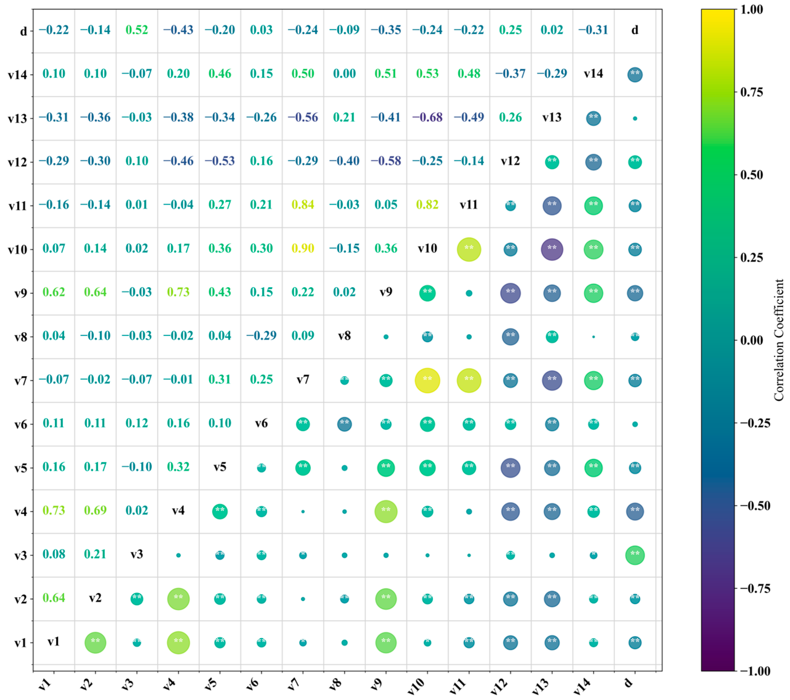
5.3.1. Selection and Correlation of Driving Factors with CCD

Given that fossil fuel consumption is the primary source of CEs, controlling fossil fuel use is essential for achieving CB and enhancing CEE [64]. Therefore, this study initially selects energy structure and energy intensity as key variables. Considering the dynamic relationship between urban CB and both CEs and CS capacity, it is crucial to examine factors influencing both carbon sources and sinks. Drawing on existing literature, this study systematically identifies potential influencing factors from both socio-economic and natural dimensions [48,65,66]. Ultimately, 13 potential influencing factors are identified: temperature (v1), precipitation (v2), forest scale (v3), population density (v4), degree of openness (v5), tech development (v6), economic development (v7), scale of the secondary industry (v8), industrial enterprise scale (v9), resident consumption (v10), urbanization (v11), government intervention (v12), energy intensity (v13), and energy structure (v14), as detailed in

Table 8. Indicators and metrics.

Indicator	Measurement Indicator	Unit
Temperature	Annual average temperature [67]	°C (degrees Celsius)
Precipitation	Annual average precipitation [67]	mm (millimeters)
Forest scale	Forest coverage rate [66]	%
Population density	Year-end registered population/administrative area land area [68]	persons/km2
Degree of openness	Total import and export/regional GDP [24]	%
Tech development	Science and technology expenditure/government fiscal expenditure [24]	%
Economic development	Per capita GDP at constant prices [59]	CNY
Scale of secondary industry	Secondary industry output/GDP [69]	%
Industrial enterprise scale	Number of industrial enterprises above a designated size [16]	count
Resident consumption	Per capita retail sales of consumer goods [69]	CNY/person
Urbanization	Urban resident population/total resident population [59]	%
Government intervention	Local government science and technology expenditure/GDP [70]	%
Energy intensity	Energy consumption per unit of GDP [16]	10,000 tons standard coal/CNY 100 million
Energy structure	Total electricity consumption [24]	100 million kWh

.

Figure 10 illustrates the correlation between CCD and these characteristic variables. Concerning natural factors, CCD demonstrates a significant negative correlation with average local temperature (r = −0.22, p < 0.01) and average precipitation (r = −0.14, p < 0.01) and a significant positive correlation with forest scale (r = 0.52, p < 0.01). In terms of socio-economic factors, CCD is significantly negatively correlated with population density (r = −0.43, p < 0.01), degree of openness (r = −0.02, p < 0.01), economic development level (r = −0.24, p < 0.01), scale of the secondary industry (r = −0.09, p < 0.01), industrial enterprise scale (r = −0.35, p < 0.01), resident consumption (r = −0.24, p < 0.01), urbanization (r = −0.22, p < 0.01), and energy structure (r = −0.31, p < 0.01), while it is significantly positively correlated with government intervention (r = 0.25, p < 0.01).

5.3.2. Model Selection and Validation

Nine commonly used machine learning algorithms were trained on the data. Hyperparameter tuning was applied using grid search to optimize model performance and generalization. To prevent overfitting on a single training set, three-fold cross-validation was employed. Root mean square error (RMSE), mean absolute percentage error (MAPE), and coefficient of determination (R²) were employed to assess model performance, with Figure 11 illustrating the outcomes for each algorithm.

In the context of regression analysis, smaller RMSE and MAE values imply better predictive accuracy, and an R² value closer to 1 represents a superior model fit. As illustrated in Figure 11, the XGBoost algorithm achieved relatively low RMSE and MAE values and the highest R² among the evaluated models. These results suggest that XGBoost provides the most accurate fit for the data. Consequently, this study utilizes the XGBoost algorithm to identify and quantify the driving factors influencing the CCD.

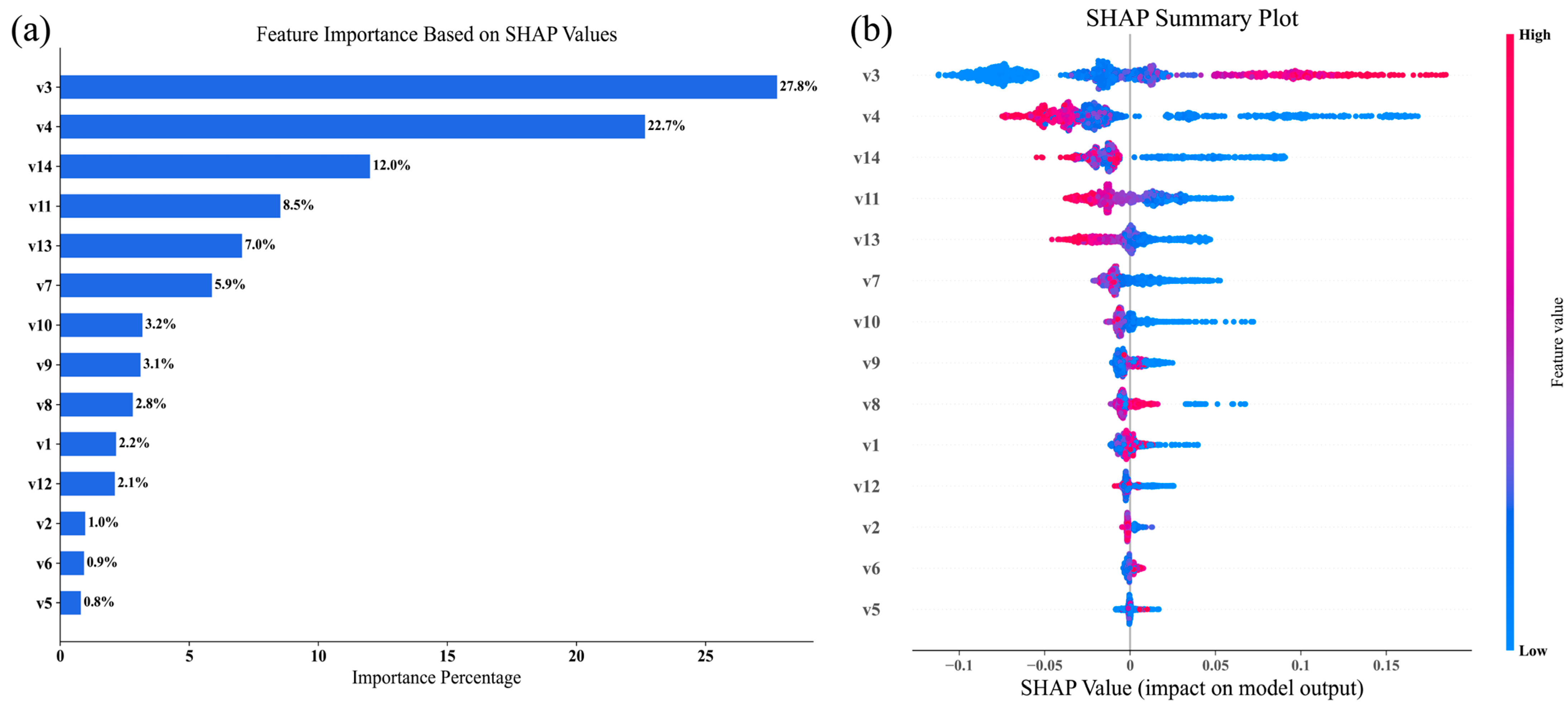
5.3.3. Identification of Key Factors

Leveraging the trained XGBoost model, this study employs the SHAP interpretability framework to evaluate the relative contribution and underlying mechanisms of each factor influencing CCD enhancement. The SHAP framework opens the XGBoost “black box,” explicitly demonstrating the relative importance of each factor and its influence direction on CCD. Inspired by Zhang et al. [71], the mean SHAP values across the full sample were computed to rank factor importance. These mean SHAP values quantify each factor’s contribution to coordinated improvements in CEE and CB and serve as a key tool for identifying major drivers. Figure 12 reports the mean SHAP values and their proportions. The horizontal axis presents mean SHAP values, and the vertical axis lists the factors. In Figure 12a, forest scale and population density exhibit the highest mean SHAP values, accounting for 27.8% and 22.7%, respectively. This result suggests that forest cover and population density are the primary drivers of CCD. Population density (v4), energy structure (v14), urbanization (v11), energy intensity (v13), and economic development level (v7) serve as secondary drivers of CCD. The SHAP values for forest coverage range between 0.00 to 0.03 and −0.01 to −0.02, with a maximum value close to 0.02, indicating that an increase in forest coverage helps improve CCD. The SHAP values for population density range from −0.01 to −0.05, showing a negative impact on CCD. The SHAP values for urbanization rate are mostly distributed between 0.00 and −0.05, suggesting that a higher urbanization rate is unfavorable for CCD improvement. The SHAP values for energy intensity are concentrated between 0 and −0.05, indicating that higher energy intensity negatively impacts CCD improvement. The impact mechanism of economic development level on CCD is complex and requires in-depth analysis using dependence plots.

5.3.4. Single-Factor Importance Impact Analysis

Figure 12b shows that red and blue data points for certain variables are distributed on both sides of the decision boundary, indicating no simple linear relationship with the CCD between CEE and CB. To further analyze these complex relationships, SHAP dependence plots from the XGBoost model and partial dependence plots were utilized (Figure 13). Figure 13a reveals that forest scale (v3) exhibits an overall increasing SHAP trend, positively influencing CCD when forest coverage exceeds approximately 0.2, reflecting forests’ role as key carbon sinks that absorb and store atmospheric CO₂, thereby enhancing CB and improving CEE. In contrast, Figure 13b shows that population density (v4) negatively correlates with CCD beyond roughly 100 persons/km² due to increased energy demand, traffic congestion, and urban expansion compressing natural CS spaces, which impedes the CCD. Figure 13c indicates that total electricity consumption (v14) negatively affects CCD above about 10 billion kWh, linked to the YRB’s coal-dependent power supply that raises CEs and may exceed natural carbon absorption capacity. Similarly, Figure 13d demonstrates that urbanization rate (v11) negatively impacts CCD when exceeding approximately 0.5, as infrastructure expansion, building material production, and transportation growth elevate energy consumption and CEs, weakening regional CEE and CB. For energy intensity (v13), Figure 13e reveals a generally declining SHAP trend with a negative effect on CCD beyond roughly 10,000 tons of standard coal per CNY 100 million, reflecting high fossil fuel reliance and associated carbon emissions. Finally, Figure 13f shows a U-shaped relationship between economic development level (v7) and CCD: per capita GDP above CNY ~25,000 initially decreases CCD due to high-carbon industries but improves with further growth and cleaner energy adoption, enhancing synergy between CEE and CB. These results underscore the complex, nonlinear mechanisms through which socio-economic and environmental factors affect the CCD in the YRB.

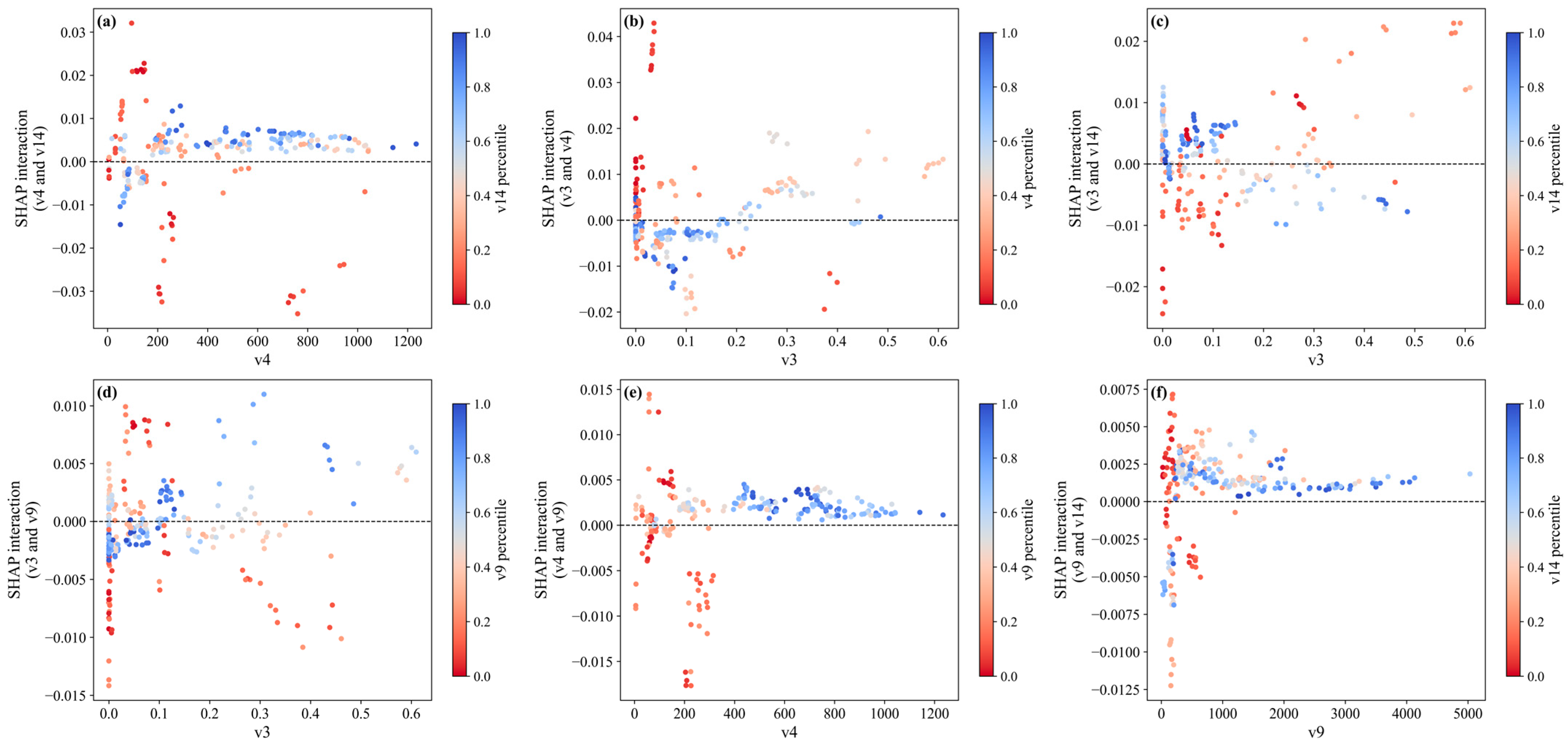
5.3.5. Interaction Analysis of Factors

To gain deeper insight into the nonlinear interaction effects of regional characteristic variables on CCD, Figure 14a–f present SHAP interaction plots for the six most influential variable pairs. Figure 14a reveals that in regions with low population density (v4) and a high share of coal-based energy (v14), interaction SHAP values are significantly negative, indicating that low-density areas may hinder energy transition and amplify the adverse effects of carbon-intensive energy structures. As shown in Figure 14b, the interaction between population density (v4) and forest coverage (v3) becomes increasingly positive with urbanization, suggesting that improved greening in densely populated areas contributes more significantly to CCD. Figure 14c illustrates that the negative impact of a coal-heavy energy structure is evident under low forest coverage but weakens as forest coverage increases, highlighting the ecological buffering role of forests. Moreover, Figure 14d indicates a strong nonlinear interaction between forest coverage (v3) and industrial enterprise scale (v9), where industrial expansion suppresses CCD in ecologically fragile areas, but this negative effect is mitigated or even reversed in areas with medium to high forest coverage, reflecting the potential of ecological–industrial synergy. Figure 14e shows that when population density is low, a larger industrial scale leads to more negative interaction effects, suggesting a mismatch with population carrying capacity. However, as density increases or industrial activity becomes more concentrated, this effect diminishes, emphasizing the regulatory role of scale–population coordination. Finally, Figure 14f reveals that regions with few industrial enterprises and a coal-dominated energy structure face strong suppression of CCD, yet as industrial activity increases, the interaction values rise toward neutrality or even become positive, indicating that industrial development may facilitate energy optimization and alleviate the negative impacts of high-carbon energy.

In summary, the SHAP interaction plots provide visual evidence of the interaction mechanisms among forests, population, energy, and industry. Within the YRB, forest coverage plays a significant buffering role against the negative impacts caused by a high-carbon power generation energy structure and industrial activities. Meanwhile, the degree of matching population density and the scale of industrial enterprises regulates the CCD of CEE and CB to varying extents. This indicates that coordinated efforts to increase forest coverage, substitute coal-fired power, and promote green upgrading of industrial enterprises are essential for systematically improving the CCD.

6. Discussion

6.1. Comparison with Previous Research

In terms of the research perspective, CEE and CB have always been key focuses in many studies. However, previous research has primarily concentrated on the interactions between the related areas of CEE and CB or explored the impact of single factors on CEE [72,73]. In contrast, this study centers on investigating the synergistic relationship between CEE and CB from a comprehensive perspective. This research approach captures the complex dynamic interactions between the systems more comprehensively than merely considering unidirectional effects.

First, from the subsystem perspective, the overall level of CB has declined [74,75]. Cities in the YRB have seen significant increases in population and urban construction land. This expansion has grown in urban space while compressing ecological land. As a result, CEs have risen, and CS have declined. Consequently, CB has decreased [29]. The upstream and midstream regions exhibit higher CB levels compared to the downstream. Upstream regions, characterized by abundant natural resources, lower development intensity, and effective ecological conservation, maintain high CB levels. Conversely, rapid economic growth in downstream cities has led to ecological land encroachment, resulting in lower ecological carrying capacities. This observation aligns with the findings reported by Dong et al. [29]. In terms of CEE, the YRB exhibited a fluctuating trend, characterized by an initial decline, a subsequent rise, and then another decline. This pattern is likely closely associated with the onset of the COVID-19 pandemic [22]. High CEE levels are concentrated in the downstream regions and upstream regions, while the midstream lags. The upstream region of the YRB relies on renewable energy sources, including wind and solar power. Although its economic scale is modest, its total energy consumption and CEs remain low. This likely explains its high CEE. Despite higher energy consumption in the downstream, advanced technology, greater economic openness [76], and ongoing industrial optimization [22,77] support elevated CEE levels. The fluctuations and decline in both may be closely related to factors such as imbalances in ecological construction and urbanization [78,79].

Second, regarding the temporal dynamics of CCD, the CCD across the YRB has generally declined, indicating low overall synergy. The midstream and upstream regions have transitioned from antagonism to moderate imbalance, while the downstream has had a consistently moderate imbalance. The region’s energy structure, predominantly fossil fuels, coupled with high electricity demand, sustains elevated carbon emissions, thereby reducing CCD [80].

Third, from the perspective of CCD’s spatial evolution, the upstream and midstream regions exhibit higher CCD levels than the downstream spatially. Previous research has highlighted spatial mismatches between CEs and CS [51]. This study further reveals spatial mismatches between CEE and CB. Downstream regions, despite the high CEE, suffer from poor CB, leading to a lower overall CCD. A significant positive spatial correlation exists in the CCD, manifesting as high-high and low-low clusters. High-high clusters are mainly in the midstream and parts of the upstream, while low-low clusters are in downstream regions like Henan and Shandong. Li et al. have drawn similar conclusions regarding high-quality urban development in the YRB [81]. Midstream and upstream benefit from rich carbon sink resources and significant carbon sequestration potential [9]. Enterprises in these regions actively optimize energy structures and promote clean energy usage, collectively enhancing CCD. In contrast, regions like Shandong and Henan, dominated by energy-intensive industries, face substantial emission reduction pressures, leading to low-level clustering [9]. Overall, CCD disparities in the YRB are narrowing, primarily due to inter-regional differences. Although no studies directly reflect this phenomenon, Wang et al.’s research on CEE in the YRB indirectly supports this trend [21]. The adoption of sustainable development concepts and regional coordination strategies has contributed to this convergence [82]. However, the probability of cities achieving leapfrog improvements in CCD remains low, with “club convergence” and the “Matthew effect” evident. This likely stems from similar regional economic conditions and institutional policies. These factors foster comparable development levels among adjacent cities [82].

Fourth, from the perspective of CCD’s driving factors, forest coverage emerges as the primary natural factor influencing CCD. Previous studies have identified forest coverage as a significant determinant of CEE [69]. This study further confirms its substantial impact on CCD. Population density ranks as the second major factor, consistent with earlier findings that population significantly affects CEs in the YRB [83]. The CCD is substantially affected by socioeconomic variables such as energy structure, industrial scale, energy intensity, and economic development, aligning with Lv et al.’s research [16]. This study additionally finds that energy structure, population density, and energy intensity negatively affect CCD, while forest coverage has a positive impact. Moreover, economic development levels exhibit a U-shaped relationship with the CCD.

6.2. Research Limitations and Future Directions

This study has several limitations that provide directions for future improvement. First, in terms of research indicators, the current CB framework mainly focuses on carbon sequestration capacity, without adequately incorporating other key ecosystem services such as biodiversity conservation, water purification, and flood regulation. To better support sustainable development in the YRB, future studies should construct a comprehensive ecosystem index integrating carbon sequestration, biodiversity, water purification, and flood regulation to enable a holistic assessment of ecological health and promote synergy between the “carbon peaking–carbon neutrality” goals and ecological security. Second, regarding research data, although this study adopts 1 km × 1 km carbon emission data to improve spatial resolution, this may still overlook emission hotspots in highly urbanized or industrialized areas. Future research could utilize higher-resolution grids (e.g., 500 m or 30 m) to enhance spatial accuracy. Third, in terms of research content, the current study emphasizes spatiotemporal evolution and driving factors of CCD from 2006 to 2022 but lacks future-oriented analysis. Scenario simulations incorporating policy measures, technological advances (e.g., CCS), and behavioral changes (e.g., renewable energy adoption) could help explore the dynamic evolution of CCD and provide policy guidance. Finally, this study is based on city-level data and lacks micro-level perspectives, limiting its relevance to SDG 10. Future studies could introduce micro-survey data to examine how improvements in CEE–CB coordination affect disadvantaged groups in terms of energy burden, employment, and income, thereby enhancing the equity dimension of dual carbon strategies.

7. Conclusions and Recommendations

7.1. Research Conclusions

This study integrates the CCD of CEE and CB in the YRB into a development framework. Using the CCD model, we measured the CCD of 74 cities in the YRB from 2006 to 2022. Kernel density estimation, spatial autocorrelation analysis, Dagum Gini coefficient, and Markov chain analysis were employed to explore the spatiotemporal evolution characteristics of CCD. Machine learning algorithms were utilized to accurately identify key factors influencing the coordination between the two. The principal findings are summarized below:

First, between 2006 and 2022, the CCD in the YRB declined from 0.41 to 0.33, with an average value of 0.36 and an annual decrease rate of approximately 1.30%. This reflects a persistently low and weakening coordination. All three regions showed a downward trend, but with distinct trajectories. The midstream region began with the highest coordination degree at 0.49 in 2006 but experienced the steepest decline, averaging 1.91 percent per year. It transitioned from a state of antagonism to moderate imbalance in 2013. The upstream region declined more gradually, at an annual rate of 1.05 percent, and surpassed the midstream in later years. It shifted to moderate imbalance in 2014. The downstream region consistently exhibited the lowest coordination level and remained in a state of moderate imbalance throughout the entire study period.

Second, the CCD in the YRB generally declined from west to east. In 2006, only Qingyang and Wuwei cities reached the “high coordination” level, while by 2022, no cities remained at this level. The number of cities classified as “moderate imbalance” significantly increased, mainly concentrated in the midstream and downstream areas. High coordination clustered in midstream and parts of upstream areas, whereas low coordination concentrated downstream. Regarding spatial autocorrelation, the CCD exhibited a significant positive spatial correlation, with high-high clustering mainly in the midstream and parts of the upstream regions, while low-low clusters are distributed in the downstream areas of Henan and Shandong provinces. The overall Dagum Gini coefficient decreased slightly from 0.197 to 0.181, indicating a modest reduction in regional inequality. Interregional differences accounted for the largest share of disparities. Midstream disparities declined, while upstream and downstream disparities rose slightly. Upstream–downstream and downstream–midstream gaps narrowed, while the upstream–midstream gap slightly widened. Markov chain analysis showed strong stability, with over 90% of cities remaining in the same coordination category, indicating limited upward mobility and weak spillover effects.

Third, forest coverage rate and population density emerged as the dominant determinants of CCD, with SHAP values accounting for 27.8% and 22.7%, respectively. Socioeconomic factors—including energy structure, industrial enterprise scale, energy intensity, and economic development—served as secondary determinants influencing CCD. Energy structure, population density, and energy intensity negatively affected CCD, while forest coverage rate positively influenced CCD. The scale of industrial enterprises and economic development level exhibited a U-shaped relationship with the CCD. From the perspective of two-factor interactions, forest coverage significantly mitigated the adverse impacts caused by high-carbon power generation energy structures and industrial activities; meanwhile, the matching degree between population density and industrial enterprise scale moderately regulates the CCD level.

7.2. Recommendations

First, enhance the coordination among the energy, industrial, and ecological sectors by establishing a collaborative governance framework involving multiple stakeholders, including the government, energy suppliers, industrial enterprises, and environmental organizations. Within this system, the government should optimize land use from the perspectives of spatial planning and industrial clustering to reduce energy consumption and transportation-related carbon emissions. Energy suppliers are responsible for accelerating the deployment of renewable energy and energy storage systems to decarbonize the energy structure. Industrial enterprises should actively participate in carbon capture and carbon trading mechanisms to improve energy utilization efficiency. Environmental organizations are expected to play a key role in ecological protection, public supervision, and social mobilization.

Second, strengthen regional coordination and interaction to narrow the gap in coordination levels between regions. On the one hand, maximize the catalytic and driving influence of cities with high CEE and CB to facilitate the development of cities with lower levels. On the other hand, cities along the YRB should leverage advantages in location, technology, and talent to strengthen regional cooperation. Upper region cities can share experiences in ecological protection and clean energy development with middle and lower region cities, while lower region cities can provide low-carbon technologies and talent support to upper and middle region cities.

Third, CCD development policies should be based on key determinants influencing coordination across the YRB. Upstream regions should enhance ecological protection, restrict unsustainable development, and safeguard the carbon sink functions of ecosystems. Midstream and downstream regions can improve carbon balance through large-scale afforestation, grassland restoration, and wetland conservation. In terms of energy, clean energy development should be promoted in upstream and midstream areas to reduce dependence on high-carbon sources, while downstream regions should focus on source control, the adoption of clean coal technologies, and carbon capture and storage. Regarding industrial structure, industrial cities should develop new energy industries to improve efficiency, whereas non-industrial cities should prioritize the development of modern services and high-tech sectors. For population density, upstream cities should increase investment in education and talent cultivation, while midstream and downstream cities should optimize urban spatial structure and transportation systems to alleviate population pressure.

References

1. Ma, D.; Hu, C.; Yan, Y.; Zhang, F.; Zhang, J.; Deng, P.; Chang, R. A comprehensive analysis of the spatiotemporal dynamics and determinants of carbon emission efficiency in China’s manufacturing sector. J. Environ. Manag. 2025, 381, 125269. [Google Scholar] [CrossRef] [PubMed]
2. Li, W.; Fang, S.; Yan, C.; Gong, W.; Wang, C. Research on the impact of digital economy on industrial carbon emission efficiency—An analysis based on spatial threshold model. J. Clean. Prod. 2025, 515, 145755. [Google Scholar] [CrossRef]
3. Jia, L.; Zhang, J.; Li, R.; Wang, L.; Wu, H.; Wang, P. Spatial correlation investigation of carbon emission efficiency in the Yangtze River Delta of China: The role of low-carbon pilot cities. Ecol. Indic. 2025, 172, 113282. [Google Scholar] [CrossRef]
4. Zhu, Y.; Lan, M. Digital economy and carbon rebound effect: Evidence from Chinese cities. Energy Econ. 2023, 126, 106957. [Google Scholar] [CrossRef]
5. Ren, X.; Xiong, R.; Ni, T. Spatial network characteristics of carbon balance in urban agglomerations—A case study in Beijing-Tianjin-Hebei city agglomeration. Appl. Geogr. 2024, 169, 103343. [Google Scholar] [CrossRef]
6. He, S.; Xu, S.; Zou, A.X. Does green technological diversification impact industrial carbon emissions efficiency? The role of technological specialisation. J. Innov. Knowl. 2025, 10, 100730. [Google Scholar] [CrossRef]
7. Lu, H.; Yao, Z.; Cheng, Z.; Xue, A. The impact of innovation-driven industrial clusters on urban carbon emission efficiency: Empirical evidence from China. Sustain. Cities Soc. 2025, 121, 106220. [Google Scholar] [CrossRef]
8. Wu, R.; Yu, G.; Cao, Y. The impact of industrial structural transformation in the Yangtze River economic belt on the trade-offs and synergies between urbanization and carbon balance. Ecol. Indic. 2025, 171, 113165. [Google Scholar] [CrossRef]
9. Yang, W.; Pan, J. How do trade-offs between ecological construction and urbanization affect regional carbon balance? A case study from China’s Yellow River Basin. Catena 2024, 247, 108534. [Google Scholar] [CrossRef]
10. Zhang, Z.; Zhu, J.; Lu, N.; Yang, L. Interaction between carbon emission efficiency and ecological environment from static and dynamic perspectives. Ecol. Indic. 2024, 158, 111436. [Google Scholar] [CrossRef]
11. Wang, C.; Guo, Y.; Shao, S.; Fan, M.; Chen, S. Regional carbon imbalance within China: An application of the Kaya-Zenga index. J. Environ. Manag. 2020, 262, 110378. [Google Scholar] [CrossRef]
12. Tang, Z.; Tang, S.; Zou, J. Administrative division adjustment and carbon intensity: Evidence from County-to-District Reform in China. Cities 2025, 160, 105833. [Google Scholar] [CrossRef]
13. Chang, X.; Li, J.; Zheng, Q. Does new-type infrastructure improve total factor carbon productivity? Experimental evidence from China. J. Clean. Prod. 2024, 460, 142620. [Google Scholar] [CrossRef]
14. Khoshnevisan, B.; Rafiee, S.; Omid, M.; Mousazadeh, H. Applying data envelopment analysis approach to improve energy efficiency and reduce GHG (greenhouse gas) emission of wheat production. Energy 2013, 58, 588–593. [Google Scholar] [CrossRef]
15. Dong, F.; Li, X.; Long, R.; Liu, X. Regional carbon emission performance in China according to a stochastic frontier model. Renew. Sustain. Energy Rev. 2013, 28, 525–530. [Google Scholar] [CrossRef]
16. Lv, T.; Geng, C.; Zhang, X.; Hu, H.; Li, Z.; Zhao, Q. Spatiotemporal evolution and influencing factors of urban industrial carbon emission efficiency in the Mid-Yangtze River urban agglomeration of China. Phys. Chem. Earth Parts A/B/C 2024, 135, 103607. [Google Scholar] [CrossRef]
17. Zhang, C.; Chen, P. Industrialization, urbanization, and carbon emission efficiency of Yangtze River Economic Belt-empirical analysis based on stochastic frontier model. Environ. Sci. Pollut. Res. Int. 2021, 28, 66914–66929. [Google Scholar] [CrossRef]
18. Shu, T.; Liao, X.; Yang, S.; Yu, T. Towards sustainability: Evaluating energy efficiency with a super-efficiency SBM-DEA model across 168 economies. Appl. Energy 2024, 376, 124254. [Google Scholar] [CrossRef]
19. Wei, Q.; Xue, L.; Zhang, H.; Chen, P.; Yang, J.; Niu, B. Spatiotemporal analysis of carbon emission efficiency across economic development stages and synergistic emission reduction in the Beijing-Tianjin-Hebei region. J. Environ. Manag. 2025, 377, 124609. [Google Scholar] [CrossRef]
20. Cai, A.; Guo, R.; Zhang, Y.; Wang, L.; Lin, R.; Wu, H.; Huang, R.; Zhang, J.; Wu, J. Assessing urban carbon health in China’s three largest urban agglomerations: Carbon emissions, energy-carbon emission efficiency and carbon sinks. Appl. Energy 2025, 383, 125326. [Google Scholar] [CrossRef]
21. Wang, J.; Liao, Z.; Sun, H. Analysis of Carbon Emission Efficiency in the Yellow River Basin in China: Spatiotemporal Differences and Influencing Factors. Sustainability 2023, 15, 8042. [Google Scholar] [CrossRef]
22. Wang, X.; Shen, Y.; Su, C. Spatial-temporal evolution and driving factors of carbon emission efficiency of cities in the Yellow River Basin. Energy Rep. 2023, 9, 1065–1070. [Google Scholar] [CrossRef]
23. Li, R.; Han, X.; Wang, Q. Do technical differences lead to a widening gap in China’s regional carbon emissions efficiency? Evidence from a combination of LMDI and PDA approach. Renew. Sustain. Energy Rev. 2023, 182, 113361. [Google Scholar] [CrossRef]
24. Dong, F.; Wang, P.; Li, W. Study on the efficiency evolution of carbon emissions and factors affecting them in 143 countries worldwide. Urban. Clim. 2025, 59, 102265. [Google Scholar] [CrossRef]
25. Huang, J.; Han, W.; Zhang, Z.; Ning, S.; Zhang, X. The decoupling relationship between land use efficiency and carbon emissions in China: An analysis using the Socio-Ecological Systems (SES) framework. Land. Use Policy 2024, 138, 107055. [Google Scholar] [CrossRef]
26. Zhao, R.; Wu, J.; Sun, J. Analysis of disequilibrium and driving factors of carbon emission efficiency: Evidence from five major urban agglomerations in China. J. Clean. Prod. 2024, 478, 143908. [Google Scholar] [CrossRef]
27. Park, G.; Kim, D. Regional carbon emission efficiency analysis and factor decomposition: Cases from South Korea. Energy Rep. 2025, 13, 903–913. [Google Scholar] [CrossRef]
28. Zhang, Z.; Jin, G. Spatiotemporal differentiation of carbon budget and balance zoning: Insights from the middle reaches of the Yangtze River Urban Agglomeration, China. Appl. Geogr. 2024, 167, 103293. [Google Scholar] [CrossRef]
29. Dong, L. Spatio-temporal evolution and prediction of carbon balance in the Yellow River Basin and zoning for low-carbon economic development. Sci. Rep. 2024, 14, 14385. [Google Scholar] [CrossRef]
30. Huang, H.; Jia, J.; Chen, D.; Liu, S. Evolution of spatial network structure for land-use carbon emissions and carbon balance zoning in Jiangxi Province: A social network analysis perspective. Ecol. Indic. 2024, 158, 111508. [Google Scholar] [CrossRef]
31. Jiang, X.; Chu, X.; Yang, X.; Jiang, P.; Zhu, J.A.; Cai, Z.; Yu, S. Spatiotemporal Dynamics of Land Use Carbon Balance and Its Response to Urbanization: A Case of the Yangtze River Economic Belt. Land. 2025, 14, 41. [Google Scholar] [CrossRef]
32. Wang, C.; Zhan, J.; Zhang, F.; Liu, W.; Twumasi-Ankrah, M.J. Analysis of urban carbon balance based on land use dynamics in the Beijing-Tianjin-Hebei region, China. J. Clean. Prod. 2021, 281, 125138. [Google Scholar] [CrossRef]
33. Cheng, Z.; Li, L.; Liu, J.; Zhang, H. Total-factor carbon emission efficiency of China’s provincial industrial sector and its dynamic evolution. Renew. Sustain. Energy Rev. 2018, 94, 330–339. [Google Scholar] [CrossRef]
34. Meng, F. Carbon emissions efficiency and abatement cost under inter-region differentiated mitigation strategies: A modified DDF model. Phys. A: Stat. Mech. Its Appl. 2019, 532, 121888. [Google Scholar] [CrossRef]
35. Shi, Y.; Wei, Z.; Shahbaz, M.; Zeng, Y. Exploring the dynamics of low-carbon technology diffusion among enterprises: An evolutionary game model on a two-level heterogeneous social network. Energy Econ. 2021, 101, 105399. [Google Scholar] [CrossRef]
36. Du, M.; Feng, R.; Chen, Z. Blue sky defense in low-carbon pilot cities: A spatial spillover perspective of carbon emission efficiency. Sci. Total Environ. 2022, 846, 157509. [Google Scholar] [CrossRef]
37. Gao, Z.; Li, L.; Hao, Y. Dynamic evolution and driving forces of carbon emission efficiency in China: New evidence based on the RBM-ML model. Gondwana Res. 2023, 116, 25–39. [Google Scholar] [CrossRef]
38. Wu, G.; Liu, X.; Cai, Y. The impact of green finance on carbon emission efficiency. Heliyon 2024, 10, e23803. [Google Scholar] [CrossRef]
39. Zhao, S.; Zhang, X. Did digitalization of manufacturing industry improved the carbon emission efficiency of exports: Evidence from China. Energy Strategy Rev. 2025, 57, 101614. [Google Scholar] [CrossRef]
40. Liu, G.; Zhang, G.; Song, M.; Fu, S. Carbon emissions trading and corporate energy efficiency: Evidence from a quasi-natural experiment in China. Technol. Forecast. Social. Change 2025, 212, 123959. [Google Scholar] [CrossRef]
41. Zhang, N.; Sun, F.; Hu, Y. Carbon emission efficiency of land use in urban agglomerations of Yangtze River Economic Belt, China: Based on three-stage SBM-DEA model. Ecol. Indic. 2024, 160, 111922. [Google Scholar] [CrossRef]
42. Zhang, J.; Yang, K.; Wu, J.; Duan, Y.; Ma, Y.; Ren, J.; Yang, Z. Scenario simulation of carbon balance in carbon peak pilot cities under the background of the “dual carbon” goals. Sustain. Cities Soc. 2024, 116, 105910. [Google Scholar] [CrossRef]
43. Panza, L.; Peron, M. The role of carbon tax in the transition from a linear economy to a circular economy business model in manufacturing. J. Clean. Prod. 2025, 492, 144873. [Google Scholar] [CrossRef]
44. van der Ploeg, F. Why green subsidies are preferred to carbon taxes: Climate policy with heightened carbon tax salience. J. Environ. Econ. Manag. 2025, 130, 103129. [Google Scholar] [CrossRef]
45. Wang, P.-T.; Zhang, Y.-X.; Wang, F.-Y.; Xu, M. Carbon capture, utilization, and storage in China’s high-emission industries: Optimal deployment under carbon neutrality goals. Energy 2025, 323, 135774. [Google Scholar] [CrossRef]
46. Li, M.; Li, F.; Qiu, J.; Zhou, H.; Wang, H.; Lu, H.; Zhang, N.; Song, Z. Multi-objective optimization of non-fossil energy structure in China towards the carbon peaking and carbon neutrality goals. Energy 2024, 312, 133643. [Google Scholar] [CrossRef]
47. Xu, G.; Zang, L.; Schwarz, P.; Yang, H. Achieving China’s carbon neutrality goal by economic growth rate adjustment and low-carbon energy structure. Energy Policy 2023, 183, 113817. [Google Scholar] [CrossRef]
48. Gao, X.; Li, S. A Dynamic Evolution and Spatiotemporal Convergence Analysis of the Coordinated Development Between New Quality Productive Forces and China’s Carbon Total Factor Productivity. Sustainability 2025, 17, 3137. [Google Scholar] [CrossRef]
49. Su, T.; Chen, Y.; Lin, B. Uncovering the role of renewable energy innovation in China’s low carbon transition: Evidence from total-factor carbon productivity. Environ. Impact Assess. Rev. 2023, 101, 107128. [Google Scholar] [CrossRef]
50. Shen, W.; Yu, X.; Sun, T.; Pan, T.; Zhong, S. The effects of internet infrastructure on carbon neutrality. Int. Rev. Econ. Financ. 2025, 99, 103964. [Google Scholar] [CrossRef]
51. Wu, J.; Liu, C.; Guo, H.; Li, P.; Sun, W. Examining intra-city carbon budget and carbon balance zoning based on firm-level big data: A case study of Nanjing, China. Ecol. Indic. 2024, 166, 112304. [Google Scholar] [CrossRef]
52. Liu, D. Convergence of energy carbon emission efficiency: Evidence from manufacturing sub-sectors in China. Environ. Sci. Pollut. Res. Int. 2022, 29, 31133–31147. [Google Scholar] [CrossRef] [PubMed]
53. Tone, K. A slacks-based measure of efficiency in data envelopment analysis. Eur. J. Oper. Res. 2001, 130, 498–509. [Google Scholar] [CrossRef]
54. Tone, K. A slacks-based measure of super-efficiency in data envelopment analysis. Eur. J. Oper. Res. 2002, 143, 32–41. [Google Scholar] [CrossRef]
55. Han, F.; Kasimu, A.; Wei, B.; Zhang, X.; Aizizi, Y.; Chen, J. Spatial and temporal patterns and risk assessment of carbon source and sink balance of land use in watersheds of arid zones in China—A case study of Bosten Lake basin. Ecol. Indic. 2023, 157, 111308. [Google Scholar] [CrossRef]
56. Ma, D.; Yan, Y.; Xiao, Y.; Zhang, F.; Zha, H.; Chang, R.; Zhang, J.; Guo, Z.; An, B. Research on the spatiotemporal evolution and influencing factors of urbanization and carbon emission efficiency coupling coordination: From the perspective of global countries. J. Environ. Manag. 2024, 360, 121153. [Google Scholar] [CrossRef]
57. Zhang, S.; Huang, C.; Li, X.; Song, M. The spatial–temporal evolution and influencing factors of the coupling coordination of new-type urbanization and ecosystem services value in the Yellow River Basin. Ecol. Indic. 2024, 166, 112300. [Google Scholar] [CrossRef]
58. Wen, H.; Zhang, Y.; Zhou, F.; Tian, X. Towards ecological sustainability: The progress and spatio-temporal evolution of green development in China. J. Clean. Prod. 2025, 492, 144912. [Google Scholar] [CrossRef]
59. Jin, Y.; Zhang, K.; Li, D.; Wang, S.; Liu, W. Analysis of the spatial–temporal evolution and driving factors of carbon emission efficiency in the Yangtze River economic Belt. Ecol. Indic. 2024, 165, 112092. [Google Scholar] [CrossRef]
60. Hu, H.; Yan, K.; Shi, Y.; Lv, T.; Zhang, X.; Wang, X. Decrypting resilience: The spatiotemporal evolution and driving factors of ecological resilience in the Yangtze River Delta Urban Agglomeration. Environ. Impact Assess. Rev. 2024, 106, 107540. [Google Scholar] [CrossRef]
61. Chen, P.; Shi, X. Dynamic evaluation of China’s ecological civilization construction based on target correlation degree and coupling coordination degree. Environ. Impact Assess. Rev. 2022, 93, 106734. [Google Scholar] [CrossRef]
62. Liu, Q.; Wu, Z.; Feng, S.; Li, M.; Deng, L.; Fan, Y.; Qian, X. Identifying the combined impact of human activities and natural factors on China’s avian species richness using interpretable machine learning methods. J. Environ. Manag. 2025, 376, 124479. [Google Scholar] [CrossRef] [PubMed]
63. Lai, Y.; Wan, G.; Qin, X. Decoding China’s new-type industrialization: Insights from an XGBoost-SHAP analysis. J. Clean. Prod. 2024, 478, 143927. [Google Scholar] [CrossRef]
64. You, J.; Dong, Z.; Jiang, H. Research on the spatiotemporal evolution and non-stationarity effect of urban carbon balance: Evidence from representative cities in China. Environ. Res. 2024, 252 Pt 1, 118802. [Google Scholar] [CrossRef]
65. Xing, P.; Wang, Y.; Ye, T.; Sun, Y.; Li, Q.; Li, X.; Li, M.; Chen, W. Carbon emission efficiency of 284 cities in China based on machine learning approach: Driving factors and regional heterogeneity. Energy Econ. 2024, 129, 107222. [Google Scholar] [CrossRef]
66. Wang, A.; Hu, S.; Li, J. Using machine learning to model technological heterogeneity in carbon emission efficiency evaluation: The case of China’s cities. Energy Econ. 2022, 114, 106238. [Google Scholar] [CrossRef]
67. Lai, J.; Qi, S.; Chen, J.; Guo, J.; Wu, H.; Chen, Y. Exploring the spatiotemporal variation of carbon storage on Hainan Island and its driving factors: Insights from InVEST, FLUS models, and machine learning. Ecol. Indic. 2025, 172, 113236. [Google Scholar] [CrossRef]
68. Li, Y.; Jiang, H.; Zhang, B.; Yao, S.; Gao, X.; Zhang, J.; Hua, C. Comparative evaluation of multi-scale spatiotemporal variability and drivers of carbon storage: An empirical study from 369 cities, China. Ecol. Indic. 2023, 154, 110568. [Google Scholar] [CrossRef]
69. Yang, G.; Cheng, S.; Huang, X.; Liu, Y. What were the spatiotemporal evolution characteristics and influencing factors of global land use carbon emission efficiency? A case study of the 136 countries. Ecol. Indic. 2024, 166, 112233. [Google Scholar] [CrossRef]
70. Cheng, H.; Wu, B.; Jiang, X. Study on the spatial network structure of energy carbon emission efficiency and its driving factors in Chinese cities. Appl. Energy 2024, 371, 123689. [Google Scholar] [CrossRef]
71. Zhang, J.; Ma, X.; Zhang, J.; Sun, D.; Zhou, X.; Mi, C.; Wen, H. Insights into geospatial heterogeneity of landslide susceptibility based on the SHAP-XGBoost model. J. Environ. Manag. 2023, 332, 117357. [Google Scholar] [CrossRef]
72. Chen, X.; Niu, Z.; Xu, Y. Impact of Income Inequality on Carbon Emission Efficiency: Evidence from China. Sustainability 2025, 17, 3930. [Google Scholar] [CrossRef]
73. Li, Q.; Zhang, P. Temporal–Spatial Characteristics of Carbon Emissions and Low-Carbon Efficiency in Sichuan Province, China. Sustainability 2024, 16, 7985. [Google Scholar] [CrossRef]
74. Ma, J.; Hao, Z.; Shen, Y.; Zhen, Z. Spatial-temporal evolution of carbon storage and its driving factors in the Shanxi section of the Yellow River Basin, China. Ecol. Model. 2025, 502, 111039. [Google Scholar] [CrossRef]
75. An, S.; Duan, Y.; Chen, D.; Wu, X. Spatiotemporal Evolution and Drivers of Carbon Storage from a Sustainable Development Perspective: A Case Study of the Region along the Middle and Lower Yellow River, China. Sustainability 2024, 16, 6409. [Google Scholar] [CrossRef]
76. Zhou, X.; Wu, D.; Li, J.; Liang, J.; Zhang, D.; Chen, W. Cultivated land use efficiency and its driving factors in the Yellow River Basin, China. Ecol. Indic. 2022, 144, 109411. [Google Scholar] [CrossRef]
77. Yang, F.; Zhen, J.; Chen, X. The Spatial Association Network Structure and Influencing Factors of Pollution Reduction and Carbon Emission Reduction Synergy Efficiency in the Yellow River Basin. Sustainability 2025, 17, 2068. [Google Scholar] [CrossRef]
78. Rong, T.; Zhang, P.; Li, G.; Wang, Q.; Zheng, H.; Chang, Y.; Zhang, Y. Spatial correlation evolution and prediction scenario of land use carbon emissions in the Yellow River Basin. Ecol. Indic. 2023, 154, 110701. [Google Scholar] [CrossRef]
79. Wang, Z.; Zeng, Y.; Wang, X.; Gu, T.; Chen, W. Impact of Urban Expansion on Carbon Emissions in the Urban Agglomerations of Yellow River Basin, China. Land 2024, 13, 651. [Google Scholar] [CrossRef]
80. Cui, Y.; Li, L.; Lei, Y.; Wu, S. The performance and influencing factors of high-quality development of resource-based cities in the Yellow River basin under reducing pollution and carbon emissions constraints. Resour. Policy 2024, 88, 104488. [Google Scholar] [CrossRef]
81. Chen, L.; Yu, W.; Zhang, X. Spatio-temporal patterns of High-Quality urbanization development under water resource constraints and their key Drivers: A case study in the Yellow River Basin, China. Ecol. Indic. 2024, 166, 112441. [Google Scholar] [CrossRef]
82. Chen, X.; Meng, Q.; Wang, K.; Liu, Y.; Shen, W. Spatial patterns and evolution trend of coupling coordination of pollution reduction and carbon reduction along the Yellow River Basin, China. Ecol. Indic. 2023, 154, 110797. [Google Scholar] [CrossRef]
83. Wu, H.; Yang, Y.; Li, W. Analysis of spatiotemporal evolution characteristics and peak forecast of provincial carbon emissions under the dual carbon goal: Considering nine provinces in the Yellow River basin of China as an example. Atmos. Pollut. Res. 2023, 14, 101828. [Google Scholar] [CrossRef]
Figure 1. The study area.
Sustainability 17 05975 g001
Figure 2. Change trend of CEE in the YRB from 2006 to 2022.
Sustainability 17 05975 g002
Figure 3. Spatial distribution patterns of CEE.
Sustainability 17 05975 g003
Figure 4. Change trend of CB from 2006 to 2022.
Sustainability 17 05975 g004
Figure 5. Spatial distribution patterns of ESC.
Sustainability 17 05975 g005
Figure 6. Change trend of CCD from 2006 to 2022.
Sustainability 17 05975 g006
Figure 7. Distribution of CCD with Kernel density estimation from 2006 to 2022. (a) KDE of CCD for the entire Yellow River Basin; (b) KDE for the upstream region; (c) KDE for the midstream region; and (d) KDE for the downstream region.
Sustainability 17 05975 g007
Figure 8. Spatial distribution patterns of CCD.
Sustainability 17 05975 g008
Figure 9. LISA agglomeration map of CCD.
Sustainability 17 05975 g009
Figure 10. Spearman correlation heatmap of eigenvalues and CCD (p < 0.05 for *, p < 0.01 for **).
Sustainability 17 05975 g010
Figure 11. Algorithm fitting results. (a) Linear Regression (LR); (b) Ridge Regression (RR); (c) Lasso Regression; (d) Decision Tree (DT); (e) Random Forest (RF); (f) Support Vector Machine (SVM); (g) K-Nearest Neighbors (KNN); (h) XGBoost (XGB); (i) LightGBM (LGBM).
Sustainability 17 05975 g011
Figure 12. SHAP value of influencing factors. (a) Bar chart showing feature importance ranking; (b) SHAP summary plot.
Sustainability 17 05975 g012
Figure 13. SHAP feature dependence plots. (a) Forest scale (v3); (b) Population density (v4); (c) Energy structure(v14); (d) Urbanization(v11); (e) Energy intensity (v13); (f) Economic development(v7).
Sustainability 17 05975 g013
Figure 14. Distribution of interaction effects of driving factors. (a) the interaction between population density (v4) and energy structure(v14); (b) the interaction between forest scale (v3) and population density (v4); (c) the interaction between forest scale (v3) and energy structure (v14); (d) the interaction between forest scale (v3) and industrial enterprise scale(v9); (e) the interaction between population density (v4) and industrial enterprise scale (v9); (f) the interaction between industrial enterprise scale (v9) and energy structure (v14). The color bar in each plot indicates the percentile of the interacting variable.
Sustainability 17 05975 g014