Optimal Planning and Techno-Economic Analysis of P2G-Multi-Energy Systems

Abstract

Multi-energy systems (MESs) are designed to convert, store, and distribute energy to diverse end-users, including those in the industrial, commercial, residential, and agricultural sectors. This study proposes an integrated optimal planning optimization model for the techno-economic assessment of an MES integrated with power-to-gas (P2G) to meet electricity, heating, and cooling requirements while enabling sustainable energy solutions. The goal of the system optimal planning is to appropriately size the MES components to minimize the total planning costs. This includes not only the investment and operation costs but also the emissions cost and the cost of energy not supplied (ENS). The study implements P2G, electricity demand response (E-DRP), and thermal demand response (T-DRP), with four distinct operational scenarios considered for optimal planning, to evaluate the benefits of adopting MESs. A comprehensive validation study is presented based on a case study farm in Nigeria, with an MES investment model developed to assess feasibility. The results show that the integration of P2G with E-DRP and T-DRP gives the best operational scenario and planning cost for this farming application integration, leading to potential savings of up to USD 2.77 million annually from the proposed MES adoption.

1. Introduction

Traditionally, energy vectors have been planned and operated separately, but there is a growing trend towards closer interactions among electricity, heating, cooling, transport, and gas networks [1]. The development of effective strategies for sustainable energy has become a matter of utmost importance. Multi-energy systems (MESs) convert, store, and distribute different types of energy to diverse end-users. MESs have the potential to exhibit technical, environmental, and economic performance advantages compared to conventional independent or isolated energy systems, both during operational implementation and in the planning phase [2]. There has been a constant growth of renewable energy sources and distributed generations, which increase the need to integrate multiple energy vectors in modern energy systems [3,4]. The effort of decarbonizing energy systems is achieved using P2G technology as an integral part of the MES. Equipped with strategies to tackle various energy sectors such as electricity, heating, cooling, and transportation, MESs stand as an alternative for energy production and planning, surpassing traditional approaches [5].

To provide sustainable solutions to the energy planning and management challenges, MESs are adopted as a technology that can improve energy efficiency and reduce energy costs by integrating multiple energy carriers, but they also pose technical, economic, and social challenges [6,7]. By adopting MESs, it becomes possible to design and manage multi-energy carriers collectively, e.g., natural gas, photovoltaics (PV), wind turbines (WTs), and active distribution networks. Furthermore, the conversion of these energy sources from one form to another can establish the MES as a highly relevant technology for energy production [2]. The optimal planning of MESs is necessary to determine the costs and sizes of MES elements. The costs, in turn, can be used for investment analysis of an MES to determine its feasibility.

In the literature, more research efforts are being shifted to the area of expansion of MESs as sustainable energy systems. The different options for investing in renewable energy-based generation are being investigated for their worthiness or optimality. The type of MES infrastructures, sizes, and locations for installation are determined to meet rising energy demands by end-users [8]. A methodology for optimizing energy balance, specifically focusing on sizing the capacities of fuel cells, combined heat and power (CHP) systems, gas boilers, and PVs, was introduced in [9]. The approach aimed to minimize the overall annual cost and emissions of the entire system, utilizing hourly electrical and thermal load profiles. An MES with various energy storage (ES) technologies was studied in [10], in which an extensive examination and comparison of the performance of existing ES systems with the MES revealed the superior capabilities of the MES. Sokolnikova et al. [11] focused on achieving the net-zero target by devising a methodology and a renewable energy controlling algorithm for the planning of generation capacity and the sizing of energy storage units, incorporating economic, ecological, technical, and social criteria. The analysis of the system indicates that investing in this project is economically appealing and notably advantageous from both social and environmental perspectives. This is attributed to the elevated and escalating prices of diesel fuel, coupled with the declining costs of batteries.

Within the vision of future energy networks [12], an energy hub (EH) is regarded as the key component of an MES, facilitating the efficient conversion, storage, and delivery of various energy carriers. Pazouki and Haghifam [13] conducted a study on the optimal planning and scheduling of EHs, examining the impact of uncertainty on demand response, wind energy, and energy storage. The outcomes revealed the ideal timing, types, and sizes of energy carriers for operation to minimize the operation, investment, reliability, and emission costs of the hub. A scenario-based methodology for the optimal operation of EH, considering uncertainties associated with WTs and PV, was presented in [14], where the energy hubs under different schemes utilize the k-means clustering algorithm, effectively reducing computational burdens without compromising accuracy. A genetic algorithm (GA)-based optimization method for a multi-vector power generation system that includes hydrogen storage is presented in [15]. These advanced technologies offer new ways to operate a grid-tied power network, enabling more effective use of intermittent renewable energy sources. This approach will promote the adoption of wind energy, hydrogen, and fuel cells in power generation.

Also, due to the current global effort to curb emissions of greenhouse gases such as $C{O}_2$ and $N{O}_2$, MESs are integrated with the power-to-gas (P2G) unit to utilize excessive energy generated from RESs to generate gaseous fuels such as hydrogen and methane. This technology stands out as a capable solution, playing a crucial role in mitigating greenhouse gas emissions [16]. Multiple applications of P2G in energy production were explored in [17], highlighting promising aspects anticipated to shape the future technical and economic evolution of electrical systems. Qin et al. [18] performed a robust optimal dispatch model for electricity, gas, and P2G. The findings suggested that the ultimate cost of robust optimization is lower when compared to deterministic optimization. A two-level bidding strategy for the coordination of P2G and renewable energy, considering its benefits and social welfare, was studied using a mixed-integer programming approach [19]. The P2G unit was coupled with an EH to produce synthetic methane, and it was observed that the P2G played a pivotal role in the reliability of the EH [20]. EH models incorporating a variety of energy sources and generation methods, accompanied by multiple energy storage devices to meet electrical, heating, and gas demands, are proposed in [21,22]. The results illustrate the efficacy of incorporating multi-carrier energy storage systems and P2G into EHs, resulting in decreased operational costs and minimizing emissions. Sun et al. [23] studied an integrated energy system with flexible load and P2G and presented an optimal dispatching model in the carbon trading market. In Zhang et al. [24], a multi-timescale security evaluation and regulation framework for integrated electricity and heat systems is presented. The proposed methodology addresses two primary challenges: (1) aligning asynchronous control commands to accommodate the system’s multi-timescale dynamics and (2) accurately characterizing the interdependence between electrical and thermal states. The former is achieved through the development of an analytical temperature mapping function, while the latter is addressed using local and global sensitivity factors across the integrated electricity and heat systems. Yang et al. [25] established an integrated energy system with a low-carbon economic dispatch model, incorporating carbon capture and storage CCS-P2G-CHP coupling to realize the recycling of carbon and reduce the energy cost.

In the recent literature, there has been a notable focus on techno-economic studies utilizing optimization models. These studies play a crucial role in understanding the complexity of energy systems and offering valuable decision support. Alizad et al. [26] explored the economic and technical viability of incorporating P2G into energy hub systems, considering future market conditions, and demonstrated that the implementation of the P2G system has positive impacts, including a reduction in emissions by approximately 17.7%, a decrease in operating costs by 14.6%, and an enhancement in the reliability of thermal loads. A techno-economic analysis of EHs, emphasizing offshore electro-fuel applications, was presented in [27], and it was observed that EHs might become foundational pillars within upcoming energy systems by enhancing the cost-competitiveness of renewable-based power. Xia et al. presented an optimal capacity planning for an integrated hydrogen MES to achieve the RES utilization of RES in industrial settings, considering consumer sides with energy trading [28]. A techno-economic feasibility analysis, exploring the use of biomass gasification in off-grid and grid-connected mini-grids to meet community-scale energy requirements, was presented in rural Uttar Pradesh, India [29]. It is worth noting that both renewable options were approximately half the cost of diesel generation. Di Micco et al. [30] performed a techno-economic feasibility analysis for an MES with a particular emphasis on the facilities of the Makkah Transport Company, which was a hybrid energy system incorporating wind power, distributed generation (DG), fuel cells, batteries, and an electrolyzer.

Energy consumption in the agricultural sector has risen due to factors such as growing global food demand, low productivity, automation in machinery, and advancements in technology [31]. Agricultural farms are frequently located in remote areas, and the use of MESs with renewable energy resources (RES) can mitigate the high costs associated with energy transmission networks (ETNs) [16]. Despite the significant potential for RES and integrated management in the agricultural sector, limited studies have been undertaken on MESs for agricultural applications. As an emerging technology for the generation, storage, and supply of different energy mixes, MESs can be an economical and eco-friendly choice for consideration when deciding on the source of farm power.

From the point of view of a farming unit, the inadequate supply of electricity, cooling, and heat for utilization can lead to high costs on fossil fuels, the loss of man-hours due to power outages, environmental pollution, and low profit turnout. The large spending on fossil fuels such as kerosene, premium motor spirit, diesel, and coal can be reduced if an energy production technology that is economical, optimally efficient, and clean is invested in such farms. MESs could provide an option to meet the energy needs of such farmsteads while minimizing the costs of energy production and supply. When integrated with a P2G system, MESs can even become an efficient, cost-effective, and cleaner source of farm energy, while reliably supplying the key electricity, heating, and cooling requirements for the farm. However, adopting an MES requires a significant investment; hence, the realistic evaluation and choice of an MES configuration for an optimal operational return over the investment time horizon is an important prerequisite.

Among the reviewed literature, there appears to be a scarcity of research seeking to comprehensively address the economic feasibility of investing in an MES. It is also observed that the vast majority of the above papers focus on short-term control and/or dispatching optimization problems, e.g., timescale of minutes or hours, while the investment planning is extended to a long-term, e.g., 20 years, for investment analysis. Additionally, studies on the evaluation of the measures of worth, such as the benefit–cost ratio (BCR), internal rate of return (IRR), and net present value (NPV), or worth to determine the viability of investing in an MES for specific use cases, such as agricultural farming units, are not available.

This paper introduces a comprehensive model for the planning optimization and techno-economic assessment of an MES integrated with P2G, electricity, and thermal demand response to meet electricity, heating, and cooling requirements and hence improve the sustainability of the whole system. A reference case study of a large farm in Nigeria is considered, aiming to exemplify and validate the model-based approach to developing an investment model to assess the viability of candidate MES configurations, based on actual energy audit data from the case study farm.

The detailed contributions of this study include

• Developing an optimization planning model and technical constraints to evaluate both the economic and technical viability of the referenced MES.
• Formulating an investment model linking optimal planning cost and the cost of fuel utilized by the case study farm. It also supports sensitivity analysis on fuel price volatility and discount rate, which is critical for long-term investment decisions in energy-intensive agricultural applications.
• Investigating the influence of P2G and DRPs in four scenarios to comprehend their effects on the sizing of components in the P2G-integrated MES and the associated planning costs. This enables incorporating sustainable energy solutions, lowering emissions (P2G), and better managing energy usage (DRPs).
• Evaluating measures of indices to ascertain the economic feasibility of investing in MESs and transitioning the energy supply of a farmstead to the specified MES. An investment model is then used to evaluate the economic viability of adopting the MES in the case study farm. This will enable stakeholders to benchmark MES investment outcomes against traditional energy supply models and support the business case for MES integration.

This research focuses on the techno-economic analysis of P2G multi-energy systems, which is a new concept of integrated sustainable energy systems, where multiple energy vectors of energy generation, storage, and demand management are coordinated to deliver clean energy to end-users. This paper contributes to several relevant sustainability subtopics, including new and renewable sources of energy, sustainable energy preservation and regeneration methods, system analysis methods, and the application of sustainability.

The structure of the paper is as follows: Section 2 presents the details of the reference P2G-MES model. The planning optimization model is contained in Section 3. Section 4 presents the investment model and a case study farm description. Section 5 presents the input data, results, and discussion. Finally, Section 6 concludes this work and presents recommendations for future research.

2. P2G-Multi-Energy Systems

A multi-energy system (MES) integrates multiple forms of energy to enhance overall efficiency and flexibility. It offers the potential to bridge the gap between energy supply and demand more effectively.

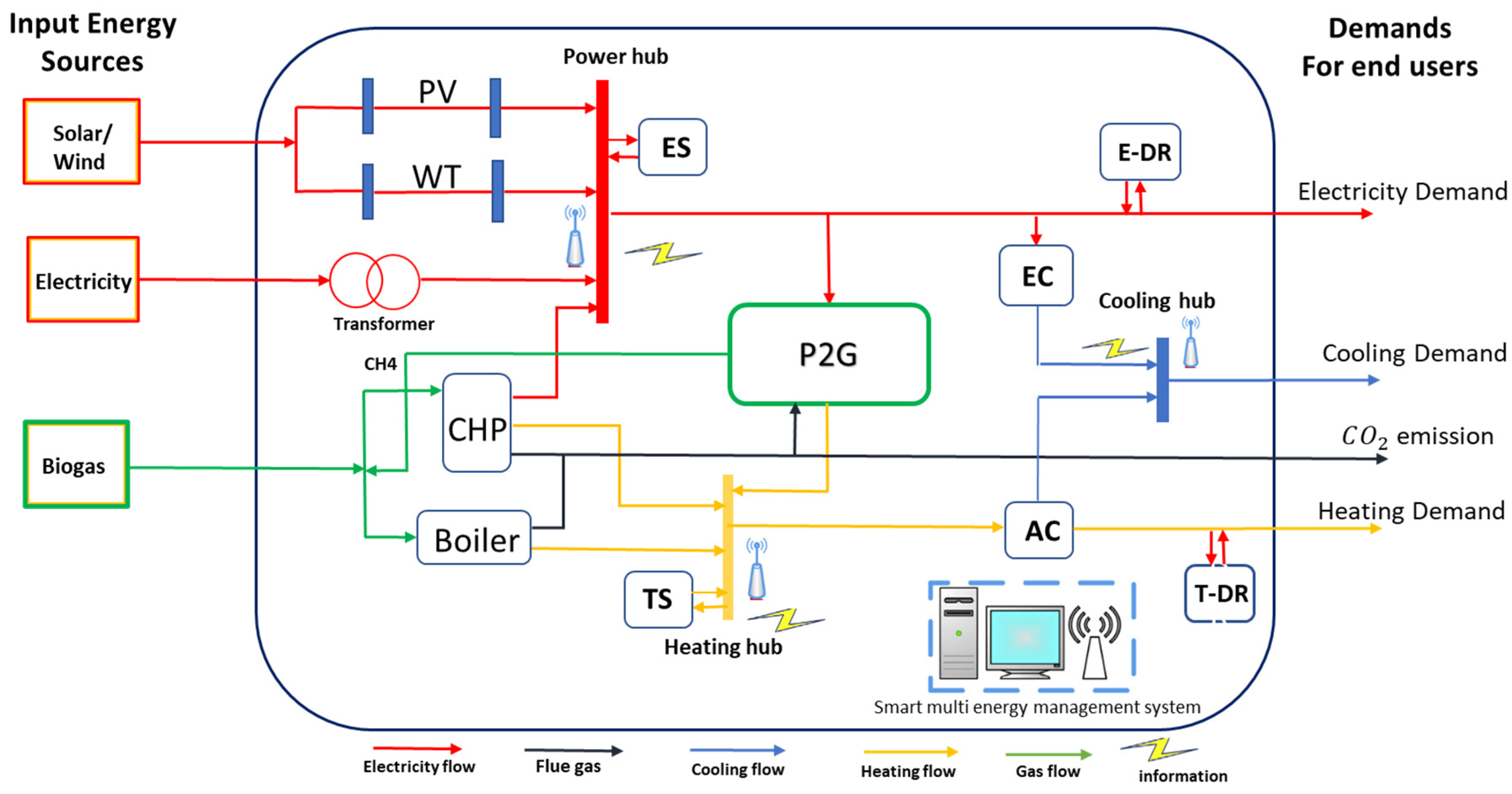
2.1. MES and Operational Concept

Figure 1 depicts an MES integrated with P2G, supplying electricity, cooling, and heat to end-users through electrical, cooling, and heating hubs.

In Figure 1, the input energy vectors include an epileptic grid power, a biogas network, RES (WTs and PV), and energy storage. Renewable sources (solar PV and WTs) generate electrical energy and connect to the power hub using AC/DC or DC/AC converters. The CHP unit is utilized to simultaneously provide electrical energy and heat, utilizing the biogas network and synthetic methane gas produced from the P2G facility. A boiler is integrated to serve as a backup source for thermal energy supplies. Absorption chillers and electric chillers are employed to meet cooling requirements, and the heat released from the P2G serves as an additional source of thermal energy for the system. The P2G unit plays a key role in the production of synthetic methane and hydrogen using the surplus electricity input to the MES and feeding to fuel the CHP unit and boiler, complementing the gas supply from the biogas network. The storage systems include thermal energy storage (TS) and electrical energy storage (ES). TS and ES can be charged and discharged, and are strategically utilized to address variations between energy supply and demand. The integration of electrical and thermal storage, along with P2G, enhances the flexibility and efficiency of the MES.

2.2. P2G Operational Concept

Figure 2 depicts the configuration of the P2G unit. To maintain an acceptable level of system stability and reliability, excess wind and solar power cannot be supplied directly to the electrical load. The P2G converts this excess electricity into methane in three primary stages, namely the electrolysis, carbon capture, and methanation processes.

The P2G unit is composed of three key sub-systems: a water electrolyzer, CO₂ capture, and methanation.

Electrolyzer: The electrolyzer involves the use of excessive electricity to split water into oxygen (O₂) and hydrogen (H₂). The excessive hydrogen can be stored in a H₂ storage and supply to the methanation process when needed. There are three primary commercial technologies for water electrolysis: proton exchange membrane electrolysis (PEM), alkaline water electrolysis (AWE), and solid oxide electrolysis (SOE) [32]. The chemical formula for the electrolysis process is expressed in Equation (1).

$$H_{2}O \to {\mathrm{H}}_2+{\displaystyle \frac{1}{2}}{\mathrm{O}}_2$$

(1)

Carbon Capture Unit: The carbon capture unit plays a pivotal role in the global energy system’s decarbonization by taking on the separation, compression, transportation, and storage of $C{O}_2$. According to the categorization in [33], $C{O}_2$ separation technologies include distillation/refrigeration, sorbent/solvent, and membrane separation. In this paper, the flue gases from the CHP and boiler are captured, and $C{O}_2$ is separated and supplied to the methanation unit.

Methanation: In this phase, hydrogen (H₂) and captured CO₂ are conveyed to the methanation unit and combined to generate methane gas. This process is highly exothermic, with the released heat utilized to fulfil a portion of the heat requirement. The chemical reaction defining the methanation stage is denoted in Equation (2).

$$C{O}_2+4H_2 \to C{H}_4+2H_{2}O+\mathrm{Heat}$$

(2)

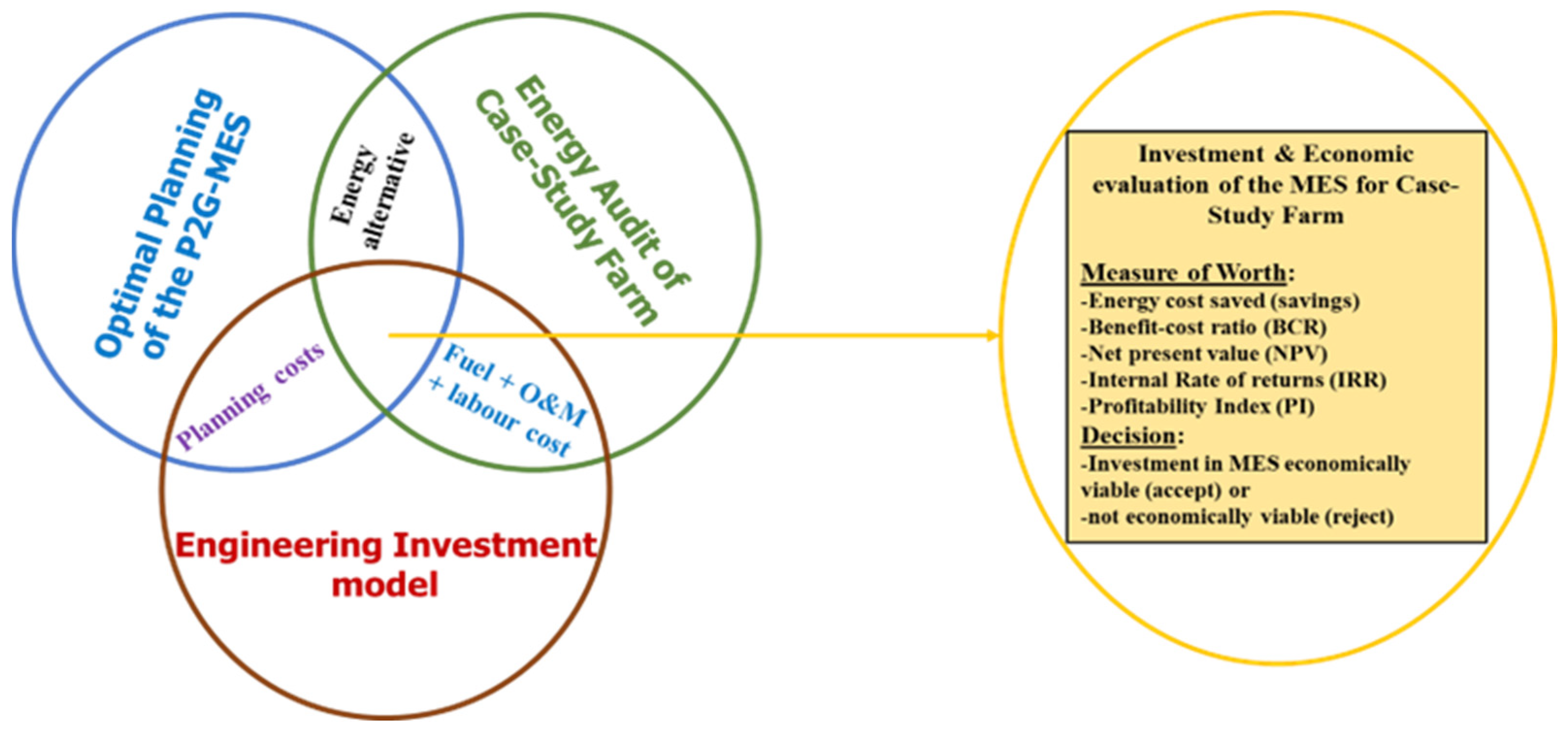
2.3. The Proposed Optimal Planning and Research Framework

This paper proposes an integrated planning and investment optimization model for the techno-economic assessment of an MES combined with P2G technology, addressing electricity, heating, and cooling demands. Figure 3 shows the core elements of the optimal planning and investment models in this research.

The detailed mathematical formulation of the planning model is presented in Section 3. The P2G-MES is optimally planned by considering three distinct scenarios, and an energy audit of a case study farm is conducted. The economic feasibility of implementing this MES and the measures of worth are evaluated against acceptable values through a case study farm (presented in Section 4).

3. MES Planning Optimization Model

The MES planning optimization takes into consideration the objective functions (OFs) and all the constraint equations that mathematically define the referenced MES configuration.

3.1. Objective Function

The objective function $\left(OF\right)$ in (3) includes costs associated with the investment $C_{INV}$, operations ($C_{OP}$), cost of reliability or energy not supplied ($C_{ENS}$), and emissions ($C_{em}$) of the MES components. Equation (4) expresses the investment cost in which $k and m$ represent two sets of MES components. The investment cost covers capital ($C_C$), replacement ($C_{RC}$), and maintenance ($C_{MC}$) costs of each MES component. The major MES components include WT, CHP, B, T, ES, TS, AC, EC, PV, and P2G, whose capacities $V^k$ are to be optimized. The minor components comprise the converter (CON) and Advanced Metering Infrastructure (AMI), whose capacities are not considered for optimization.

$$Min: OF=C_{Inv}+C_{OP}+C_{ENS}+C_{em}$$

(3)

$$\begin{gathered} C_{Inv}={\displaystyle \sum }_{kϵS}[V^k\left[C_{CC}^k+C_{RC}^k{K}_k\left(ir,N_k,r^k\right)+C_{MC}^{k}PWA\left(ir,N\right)\right] \\ +{\displaystyle \sum }_{mϵ\left\{CON,AMI\right\}}\left[C_{CC}^m+C_{RC}^m{K}_m\left(ir,N_m,r^m\right)+C_{MC}^{m}PWA\left(ir,N\right)\right] \end{gathered}$$

(4)

where

• Index $kϵS=\left\{WT,CHP,B,T,ES,TS,AC,EC,PV,P2G\right\}$ are set of major components associated with variable $V^k$;
• Index $mϵ\left\{CON, AMI\right\}$ are set of minor components that are not associated with the decision variable $V^k$;
• $V^k$ = needed capacity of component k;
• $C_{CC}^{k/m}$ = capital cost of the MES components;
• $C_{RC}^{k/m}$ = replacement cost of components k and m;
• $C_{MC}^{k/m}$ = maintenance cost of components k and m;
• $K_{k/m}$ = single payment present worth of the respective MES component;
• $ir$ = real interest rate;
• $N_{k/m}$ = economics of components k and m;
• $r^{k/m}$ = replacement number of components k and m;
• PWA = present worth annual payment.

  $$\begin{gathered} C_{OP}=PWA\left(ir,N\right)\{{\displaystyle \sum }_{t=1}^{24}{c}_e^{Net,t}{P}_e^{Net,t}+c_{biogas}^{Net} P_{biogas}^{Net,t} \\ +{\displaystyle \sum }_{sϵS}{c}_s\left(P_s^{in,t}+P_s^{out,t}\right)+{\displaystyle \sum }_{dϵ\left\{edr,hdr\right\}}{c}_d\left(P_d^{shd,t}+P_d^{shup,t}\right)\} \end{gathered}$$

  (5)

  where
• $kϵR=\left\{TS,ES,P2G\right\}$ set of storage operations components within the MES architecture
• $dϵ\left\{edr, hdr\right\}$ demand response program with shedding and shifting power;
• $c_e^{Net,t}$, $c_{biogas}^{Net}$ = price of electricity at time slot t and that of biogas network, respectively;
• $P_e^{Net,t}$, $P_{biogas}^{Net,t}$ = purchased electricity and biogas power from network at time slot t, respectively;
• $c_s$ and $c_d$ = cost coefficients associated with storage and demand response operations;
• $P_s^{in,t}, P_s^{out,t}$ = charged and discharge energies of storage devices at time slot t, respectively;
• $P_d^{shd,t}, P_d^{shup,t}$ = shifting down and shifting up energies at time slot t, respectively.

In Equation (6), $c_e^{ENS}$ denotes the price of electricity not supplied (ENS). $P_e^{ENS}$ denotes electricity not supplied (ENS). In Equation (7), $C_{em}$ expresses the emissions cost of $C{O}_2$, $N{O}_2$, and $S{O}_2$. $c_{em}$ denotes the cost for emission. The emission factors of the electricity network, boiler, and CHP are denoted by $E{F}_{em}^{Net}$, $E{F}_{em}^B$, and $E{F}_{em}^{CHP}$, respectively. $“\mathrm{if} \mathrm{and} r_{no}”$ represents the annual inflation and nominal interest rates, respectively, in (8). $r^{k/m}$ is the replacement number of components. $t$ represents time in hours. $PWA$ and $K_{k/m}$ in (9) and (10) are the present annual payment worth and single payment present worth, respectively, of the MES components.

$$C_{ENS}=\left\{PWA\left(ir,N\right)\left(c_e^{ENS}{P}_e^{ENS,t}\right)\right\}$$

(6)

$${\mathrm{C}}_{\mathrm{em}}=PWA\left(ir,N\right)\{{\displaystyle \sum }_{em=1}^3{c}_{em}(E{F}_{em}^{Net}{P}_{biogas}^{Net,t}+E{F}_{em}^{CHP}{P}_g^{NetCHP,t}+E{F}_{em}^B{P}_g^{NetB,t})\}$$

(7)

$$ir={\displaystyle \frac{\left(i{r}_{no}-if\right)}{1+if}}$$

(8)

$$PWA\left(ir,N\right)={\displaystyle \frac{{\left(1+if\right)}^N-1}{ir{\left(1+if\right)}^N}}$$

(9)

$$K_{k/m}={\displaystyle \sum }_{k/m=1}^N{\displaystyle \frac{1}{ir{\left(1+if\right)}^{r_{k/m}{N}_{k/m}}}}$$

(10)

3.2. Wind and Solar Power Models

The production of WTs is contingent on the rated power of the wind turbine $P_r^{WT}$ and the wind speed $u$. The electricity generation begins when the wind speed reaches the cut-in speed $u_{ci}$ and continues at the rated speed $u_r$. Once the wind speed is lower than the cut-in speed or exceeds the cut-out speed $u_{co}$, the turbine is deactivated. Parameters associated with the characteristics of the wind turbine are x, y, and z [34]. Equation (11) formulates the output power of WT as a function of wind speed, as follows

$${\mathrm{P}}_{\mathrm{k},\mathrm{e}}^{\mathrm{out},\mathrm{t}}=\left\{\begin{array}{c}0 \mathrm{u}<{\mathrm{u}}_{\mathrm{ci}} \\ {\mathrm{P}}_{\mathrm{r}}^{\mathrm{WT}}\left(\mathrm{z}-\mathrm{yu},\mathrm{t}+{\mathrm{xu}}^2,\mathrm{t}\right) {\mathrm{u}}_{\mathrm{ci}}\le \mathrm{u}<{\mathrm{u}}_{\mathrm{r}}\\ {\mathrm{P}}_{\mathrm{r}}^{\mathrm{WT}} {\mathrm{u}}_{\mathrm{r}}\le \mathrm{u}<{\mathrm{u}}_{\mathrm{co}} \\ 0 \mathrm{u}\ge {\mathrm{u}}_{\mathrm{co}}\end{array}\right.$$

(11)

The power output of the PV panel can be expressed in Equation (12) [6].

$$P_{k,e}^{out,t}={\eta }_{in}\times N{V}_k\times P_{STC}\times {\displaystyle \frac{I_{rad,t}}{I_{STC}}}\left[1+0.005\left(T_a-25\right)\right]$$

(12)

where ${\eta }_{in}$ is the conversion efficiency of the PV inverter, $N{V}_k$ is the number of PV modules, $I_{rad}$ is the solar radiation intensity at a given time, $I_{STC}$ represent the irradiance intensity at standard conditions (i.e., at a cell temperature of 25 °C and irradiance = 1000 W/m²), $P_{STC}$ is the rated power of the PV modules, and $T_a$ is the ambient temperature.

3.3. Constraints

3.3.1. Energy Balance Constraints

The MES must satisfy the energy balance, including electricity balance, heat balance, cold balance, and gas flow balance. The energy balance is expressed in Equations (13)–(16). For each equation, the term on the left-hand side represents the sum of output powers of all the loads at time t. Electrical loads include battery charging, converters and heaters, power shifting up, coolers, and load demand for end-users. Heating loads include heat storage charging, cooling devices, heat shifting up, and heat demand for end-users. Cooling loads are satisfied with absorption and electric chillers, while for the gas balance, imported gas from the gas utility and P2G are used to supply the CHP and boiler.

$${\displaystyle \sum }_{k=1}^{{\delta }_e }{P}_{k,e}^{out,t}={\displaystyle \sum }_{l=1}^{L_e}{P}_e^{l,t}$$

(13)

$${\displaystyle \sum }_{k=1}^{{\delta }_h}{P}_{k,h}^{out,t}={\displaystyle \sum }_{l=1}^{L_h}{P}_h^{l,t}$$

(14)

$${\displaystyle \sum }_{k=1}^{{\delta }_c}{P}_{k,c}^{out,t}={\displaystyle \sum }_{l=1}^{L_c}{P}_c^{l,t}$$

(15)

$${\displaystyle \sum }_{k=1}^{{\delta }_g}{P}_{k,g}^{out,t}={\displaystyle \sum }_{l=1}^{L_g}{P}_g^{l,t}$$

(16)

where

• ${\delta }_e$, ${\delta }_h$, ${\delta }_c$, and ${\delta }_g$ are the numbers of electricity generation, heating, cooling, and gas devices, respectively.
• L is the index of loads.
• $L_e$, $L_h$, $L_c$, and $L_g$ are the numbers of electrical, heating, cooling, and gas loads, respectively.
• $P_{k,e}^{out,t}$ represents the output electrical power of device k, which includes the energy converter, renewable generation, and electricity storage device at time slot t.
• $P_e^{l,t}$ denotes the power of electrical loads at time t, and likewise for heating, cooling, and gas balance.

3.3.2. Energy Networks Constraints

The electricity and biomethane gas bought from the networks are constrained by network capacities. ${\mathrm{P}}_{\mathrm{e}}^{\mathrm{Netmax}}$ and ${\mathrm{P}}_{\mathrm{g}}^{\mathrm{Netbioch}4}$ are the maximum capacities of power and biogas networks, respectively, in (17) and (18).

$$0\le P_e^{Net}\left(t\right)\le P_e^{Netmax}$$

(17)

$$0\le P_{biogas}^{Net}\left(t\right)\le P_{biogas}^{Netmax}$$

(18)

3.3.3. Energy Converter Constraints

The energy purchased from power and biomethane gas networks for the CHP and boiler, and the generated methane gas from P2G, must be constrained by the capacities of the converter components as expressed in Equation (19).

$${\eta }_{k,i}{P}_{k,i}^t\le V^k$$

(19)

where $i$ is the index of energy type, $k$ is the index of converter components, ${\eta }_{k,i}$ = denotes the energy efficiency associated with each component $k$, $P_{k,i}^t$ = represents the energy input for each component $k$, and $V^k$ = is the capacity limit of component $k$.

3.3.4. MES Component Constraints

The indicated capacities of the MES components are represented by $V^k$, with k representing T, CHP, B, WT, ES, TS, AC, EC, P2G, and PV. The capacities of the MES components must adhere to the maximum allowable limits $V^{kmax}$ set for each component within the hub as expressed in (20).

$$V^k\le V^{kmax}$$

(20)

where $V^k$ is the capacity of component $k$, and $V^{kmax}$ is the maximum allowable capacity of each component.

3.3.5. Operational Constraints of Energy Storage Devices

The energy storage is responsible for storing excess energy generated and discharging energy when the supply decreases. The operation of the energy storage is determined by the energy available from the previous time, the amount of energy charged and discharged in the current time $t$, and the associated energy losses. Equation (21) represents the available energy $P_{k,i}^t$, which is determined by the available energy from the previous hour $P_{k,i}^t\left(t-1\right)$, the energy charged $P_{k,i}^{in,t}$ and discharged $P_{k,i}^{out,t}$ in the current hour, and the energy losses $P_{k,i}^{loss,t}$ of the storage device. The energy loss $P_{k,i}^{loss,t}$ from storage device $k$ in time $t$ is calculated according to Equation (22). The available energy must adhere to the minimum and maximum limits specified in Equation (23). ${\alpha }_{k,i}^{min}$ and ${\alpha }_{k,i}^{max}$ are factors representing the minimum and maximum ratios of the energy capacity of the energy storage system. The charge $P_{k,i}^{in,t}$ and discharge $P_{k,i}^{out,t}$ energy are also constrained in Equations (24) and (25), respectively. Binary variables $I_{k,t}^{in,t}$ and $I_{k,t}^{out,t}$ associated with storage device $k$ in time slot $t$ are in Equation (26) to control the charging and discharging operations of the storage system, ensuring they do not occur simultaneously. The charge and discharge efficiencies are denoted by ${\eta }_{k,i}^{in}$ and ${\eta }_{k,i}^{out}$, respectively.

$$P_{k,i}^t=P_{k,i}^t\left(t-1\right)+P_{k,i}^{in,t}-P_{k,i}^{out,t}-P_{k,i}^{loss,t}$$

(21)

$$P_{k,i}^{loss,t}={\alpha }_k^{loss}{P}_{k,i}^t$$

(22)

$${\alpha }_{k,i}^{min}{P}_{k,i}\le P_{k,i}^t\le {\alpha }_{k,i}^{max}{P}_{k,i}$$

(23)

$${\alpha }_{k,i}^{min}{\eta }_{k,i}^{in}{P}_k{I}_{k,i}^{in,t} \le P_{k,i}^{in,t}\le {\alpha }_{k,i}^{max}{\eta }_{k,i}^{in}{P}_k{I}_{k,i}^{in,t}$$

(24)

$${\alpha }_{k,i}^{min}{\eta }_{k,i}^{out}{P}_k{I}_{k,i}^{out,t} \left(t\right)\le P_{k,i}^{out,t}\le {\alpha }_{k,i}^{max}{\eta }_{k,i}^{out}{P}_{k}I{k}_{k,i}^{out,t}$$

(25)

$$0\le I_{k,t}^{in,t}+I_{k,t}^{out,t}\le 1$$

(26)

3.3.6. P2G Constraints

P2G technology is utilized to transform electricity into synthetic gas, which is stored and injected into the energy hub to meet the gas demand, including the fuel requirements of the CHP and boiler units. The actual quantity of gas generated by the P2G unit in real time is represented by Equation (27). The current capacity of the P2G’s natural gas storage system is calculated similarly to previous storage systems in Equation (28). The conversion of electricity into methane by the P2G unit is limited by bounds defined in Equations (29) and (30). The storage of natural gas is subject to minimum and maximum limits, specified in Equation (31). Constraint (32) ensures that the initial state (t = 0) and final state (t = 24) of the P2G system satisfy an equality condition. The heat released by P2G is expressed in Equation (33).

$$G_{P2G}^t={\eta }_{P2G}{P}_{eP2G}^t/HH{V}_{CH4}$$

(27)

$$SO{C}_{P2G}^t=SO{C}_{P2G}\left(t-1\right)+G_{P2Gch}^t-G_{P2Gdch}^t$$

(28)

$$0=l=P_{eP2G}^t=l=P_{eP2Gmax}$$

(29)

$$0=l=G_{P2G}^t=l=G_{P2Gmax}$$

(30)

$$SO{C}_{P2Gmin}=l=SO{C}_{P2G}^t=l=SO{C}_{P2Gmax}$$

(31)

$$SO{C}_{P2G}\left(t=0\right)=l=SO{C}_{P2G}\left(t=24\right)$$

(32)

$$H_{P2G}^t=e=LH{V}_{CH4}{G}_{P2G}^t$$

(33)

3.3.7. Energy Demand Response Constraints

The energy demand increases during peak hours and drops during valley hours. Within 24 h, the aggregate amount of energy demand increase, i.e., shift-up energy, should be equal to the total amount of energy demand reduction, i.e., shift-down energy, as specified in Equation (34); $P_{k,t}^{shup,t}$ and $P_{k,i}^{shd,t}$ represent the shift-up and shift-down of $i$ energy demands by component $k$ at time slot $t$, respectively. $LP{F}_{k,i}^{shup,t}$ and $LP{F}_{k,i}^{shd,t}$ denote the $i$ energy participation factors for shifting up and shifting down component $k$ at time slot $t$, respectively. Energy demand can be adjusted upwards and downwards using Equations (35) and (36), respectively. Binary variables for shifting up $I_{k,i}^{shup,t}$ and shifting down $I_{k,i}^{shd,t}$ are expressed in Equation (37).

$${\displaystyle \sum }_{t=1}^{24}{P}_{k,i}^{shup,t}={\displaystyle \sum }_{t=1}^{24}{P}_{k,i}^{shd,t}$$

(34)

$$0\le P_{k,i}^{shup,t}\le LP{F}_{k,i}^{shup,t}$$

(35)

$$0\le P_{k,i}^{shd,t}\le LP{F}_{k,i}^{shd,t}$$

(36)

$$0\le I_{k,i}^{shup,t}+I_{k,i}^{shd,t}\le 1$$

(37)

3.3.8. ENS Constraints

The electricity not supplied constraint is modelled in Equation (38). The equivalent loss factor (ELF) is calculated by dividing the energy not supplied $P_e^{ENS}$ by the electricity demand $L_e$. The ELF value needs to be limited by a maximum threshold, as specified in Equation (39).

$${\epsilon }_L={\displaystyle \frac{1}{T}} {\displaystyle \sum }_{t=1}^{24}{\displaystyle \frac{P_e^{{ENS}^t}}{L_e^t}}$$

(38)

$${\epsilon }_L\le {\epsilon }_{Lmax}$$

(39)

${\epsilon }_L$ = the equivalent loss factor.

4. The Case Study Farm and Investment Model

Established in 2010, Songhai Rivers Farm in Tai LGA, Rivers State, Nigeria, spans 314 hectares—20 times larger than its prototype in the Benin Republic [35]. It hosts approximately 10,000 poultry fowl, 800 pigs, 500 cattle, 700 sheep, and 25 fishponds. The farm also includes large fruit plantations, offices, a 100-seat conference hall, storage units, and a hotel with 15 executive rooms. Energy needs are met by a 250 kVA diesel generator, consuming 1330 L daily, alongside other fuels like PMS, kerosene, coal, charcoal, and biogas. Despite being connected to an unreliable grid, the farm relies heavily on fossil fuels for its operations.

This section presents an energy audit and investment model to evaluate the amount of energy utilized by the farm and the cost in monetary terms. It is the key information for the investment analysis of the MES. The monthly cost of energy in the farm for the $j^{th}$ fuel type is determined by Equation (40). The energy usage is modelled in Equation (41), and the unit energy cost is calculated using Equation (42).

$$C_j={\pi }_j\times {\mathrm{Q}}_{\mathrm{j}}$$

(40)

$$E_j=HH{V}_j\times Q_j$$

(41)

$${\lambda }_j={\displaystyle \frac{C_j}{E_j}}$$

(42)

where j is the index of energy type, $C_j$ is the monthly cost of energy/fuel, $E_j$ is the energy consumed in a month, ${\lambda }_j$ denotes unit cost of fuel/energy per month, $Q_j$ is the quantity of fuel consumed by the farm per month (MJ), and $HH{V}_j$ is the heating value of the fuel consumed (in MJ/kg). The heating value of biogas in this work is taken to be 35.8 MJ. The total optimal planning costs of the MES are given in (43). The annual cost incurred by the case study farm is expressed in (44). The fuel cost is indicated in (45).

$$C_{Inv}+C_{OP}+C_{ENS}+C_{em}=C_{Total}$$

(43)

$${\pi }_{labour}+{\pi }_{o\&m}+{\pi }_{fuel}={\pi }_{Total}$$

(44)

$${\pi }_{fuel}={\pi }_{fwood}+{\pi }_{coal}+{\pi }_{diesel}+{\pi }_{pms}+{\pi }_{kero}$$

(45)

where the subscripts $Inv$, $OP$, $ENS$, $em$, $k$, and $o\&m$ stand for investment, operations, energy not supplied, emissions, the particular year, and operations and maintenance, respectively.

The present value (P) is all future values discounted to the present value. It is expressed in Equation (46) [36]. The present worth (P) given is the present value that is equivalent to the annuity with disbursements or expenses ($D_d$) or receipts or revenues $\left(R_r\right)$ in the amount A at an interest rate $i$ and within the period $N$ in years. The net present value (NPV) is expressed in Equation (47).

$$P_{R_r} or P_{D_d}=A\left({\displaystyle \frac{P}{A}},i,N\right)=R_r\left({\displaystyle \frac{{\left(1+i\right)}^N-1}{i{\left(1+i\right)}^N}}\right) or D_d\left({\displaystyle \frac{{\left(1+i\right)}^N-1}{i{\left(1+i\right)}^N}}\right)$$

(46)

$$NPV=\left(\left(P_{R_r}\right)-\left(P_{Inv}+P_{D_d}\right)\right)$$

(47)

where $P_{R_r}$, $P_{D_d}$, and $P_{Inv}$ are the present value of revenues, disbursements, and investment costs, respectively. $i$ is the interest rate, N is the lifetime, A is the annuity, and P is the present value. $R_r$ is the revenue and $D_d$ represent disbursements.

Internal rate of return (IRR) is considered the interest rate that renders the present worth or annual worth of a cash flow series precisely equal to zero. It is expressed in Equation (48).

$$\left({\displaystyle \frac{P}{A}},i\%,N^{th}\right)={\displaystyle \frac{R_r-D_d}{P_{Inv}}}$$

(48)

The benefit–cost ratio (BCR) is expressed in Equation (49), and the profitability index is given in Equation (50).

$$BCR={\displaystyle \frac{P_{R_r}}{P_{Inv}+P_{D_d}}}$$

(49)

$$PI={\displaystyle \frac{P_{R_r}-P_{D_d}}{P_{Inv}}}$$

(50)

5. Results and Discussion

5.1. Input Data

The input data on heat, electricity, and cooling demands of the MES and the price of electricity purchased from the grid network, wind speed, and solar radiation intensity are from [6,13] and shown in

Table 1. Heat, electricity, and cooling demands, hourly electricity price, wind speed, and solar radiation input data for the MES [6,13].

Time (h)	1	2	3	4	5	6	7	8	9	10	11	12	13	14	15	16	17	18	19	20	21	22	23	24
Lh	281	281	203	201	185	154	150	277	205	203	346	346	205	203	193	150	158	203	199	201	281	281	203	201
Le	606	469	503	421	401	401	418	599	603	500	599	702	705	699	798	805	801	856	1202	1202	1202	1120	775	733
Lc	1428	1266	1232	1365	1478	1633	2118	2308	2491	2744	3061	3124	3145	2963	2710	2352	2043	2170	2494	2185	1918	1750	1722	1666
λ	6.18	6.88	6.18	6.81	7.27	8.6	7.74	6.03	7.27	8.83	10.9	12.1	11.6	11.8	10.9	14.5	16.8	14.7	19.2	20	20.5	16.9	14.3	13.7
Lwd	13.7	13.3	12.3	10.9	10.4	9.94	8.46	7.97	7.52	7.64	7.77	7.44	7.36	6.95	6.7	6.91	5.19	9.53	8.18	8.3	9.16	10.6	12.8	13.9
Irad	5	10	10	11	13	50	195	305	410	520	550	650	610	520	410	305	196	50	13	12	11	10	10	5

. In the investment analysis, for the case study of Songhai Farm, located in Nigeria, a developing country, there is a significant ongoing investment in capital projects funded through loans. As of April 2025, Nigeria’s benchmark interest rate stands at 27.50% and is expected to remain at this level through the end of the quarter [37]. This rate is commonly used as a reference for many local investments. It is also noted that the rate is stable at around 13.5–14% in the period between 2016 and 2020 prior to the COVID-19 pandemic. Thus, the rate of 14% is used as a baseline discount rate in the case study. The MES lifespan is assumed to be 20 years.

In Table 1, input parameters in the first column include:Heat demand (Lh) (kWh), electricity demand (Le) (kWh), cooling demand (Lc) (kWh), electricity price (λ) ($/kWh), wind speed (Lwd) (m/s)), solar radiation (Irad) (kWh/m²).

Simulation input parameters pertaining to technological and economic information about the MES components are presented in

Table A1. Input parameters for the multi-energy system optimal planning.

Parameter	Value	Parameter	Value	Parameter	Value	Parameter	Value	Parameter	Value
$E{F}_{em}^{Netc{o}_2}$	1.432	$E{F}_{em}^{NetSs}$	0.454	$E{F}_{em}^{Netn{o}_2}$	21.8	$E{F}_{em}^{CHPc{o}_2}$	1.596	$E{F}_{em}^{CHPs{o}_2}$	0.008
$E{F}_{em}^{CHPn{o}_2}$	0.440	$E{F}_{em}^{Bc{o}_2}$	1.755	$E{F}_{em}^{BS{o}_2}$	0.011	$E{F}_{em}^{Bn{o}_2}$	0.62	${\epsilon }_{Lmax}$	0.01
$LP{F}_h^{shup}$	0.1	$LP{F}_h^{shd}$	0.1	$LP{F}_e^{shup}$	0.1	$LP{F}_e^{shd}$	0.1	$G_{P2Gmax}$	50
$P_{e_{P2Gmax}}$	50	$SO{C}_{P2Gmax}$	800	$if$	0.12	$i{r}_{no}$	0.14	$ir$	0.0179
${\eta }_{ee}^T$	0.9	${\eta }_{pv}$	0.157	${\eta }_e^{CON}$	0.9	${\eta }^{P2G}$	0.75	${\eta }_{gh}^B$	0.85
${\eta }_{gh}^{CHP}$	0.3	${\eta }_{ge}^{CHP}$	0.45	${\eta }_{EES}^{ch}$	0.9	${\eta }_{EES}^{dch}$	0.9	${\eta }_{TES}^{ch}$	0.9
${\eta }_{TES}^{dch}$	0.9	$A^{CHP}$	0.96	$A^{Net}$	0.70	$A^{WT}$	0.96	$y$	0.01
$z$	0.03	$x$	0.07	$CO{P}_{AC}$	0.7	$CO{P}_{EC}$	3.5	$T_a$	1
$r^{PV}$	3	$r^{P2G}$	1	$r^{CON}$	2	$r^{AMI}$	1	$r^{EC}$	1
$r^{AC}$	1	$r^{TES}$	2	$r^{EES}$	2	$r^T$	1	$r^B$	1
$r^{CHP}$	1	$r^{WT}$	1	$C_C^{CON}$	550	$C_C^{WT}$	2000	$C_C^{AC}$	950
$C_C^{TS}$	800	$C_C^{EES}$	1000	$C_C^T$	900	$C_C^B$	500	$C_C^{CHP}$	2500
$C_C^{EC}$	850	$C_C^{AMI}$	270	$C_C^{P2G}$	680	$C_C^{PV}$	1300	$C_{RC}^{AC}$	400
$C_{RC}^{EC}$	400	$C_{RC}^{PV}$	2500	$C_{RC}^{P2G}$	598	$C_{RC}^{CON}$	700	$C_{RC}^{AMI}$	400
$C_{RC}^{EES}$	1000	$C_{RC}^B$	300	$C_{RC}^{TES}$	600	$C_{RC}^T$	700	$C_{RC}^{WT}$	4000
$C_{MC}^{EC}$	0.16	$C_{MC}^{AMI}$	0.012	$C_{MC}^{CON}$	10	$C_{MC}^{P2G}$	68	$C_{MC}^{AC}$	0.13
$C_{MC}^{PV}$	3	$C_{MC}^{TES}$	0.01	$C_{MC}^{EES}$	10	$C_{MC}^B$	0.012	$C_{MC}^T$	0.012
$C_{MC}^{CHP}$	0.03	$C_{MC}^{WT}$	50	$I_{STC}$	1000	$N_{PV}$	15	$N_{WT}$	15
$N_{CHP}$	20	$N_B$	20	$N_T$	20	$N_{AMI}$	15	$N_{P2G}$	20
$N_{CON}$	15	$N_{EES}$	10	$N_{AC}$	20	$N_{TES}$	20	$N$	20
$V^{ACmax}$	600	$V^{ECmax}$	400	$V^{P2Gmax}$	1000	$V^{PVmax}$	2000	$V^{Tmax}$	900
$V^{TESmax}$	500	$V^{EESmax}$	400	$V^{WTmax}$	4200	$V^{Bmax}$	700	$V^{CHPmax}$	800
$LH{V}_{CH4}$	35.8	$SO{C}_{P2G0}$	120	${\alpha }_h^{min}$	0.1	${\alpha }_h^{max}$	0.9	${\alpha }_{TES}^{loss}$	0.02
${\alpha }_e^{min}$	0.1	${\alpha }_e^{max}$	0.9	${\alpha }_{EES}^{loss}$	0.02	$P_{STC}$	0.25	$NSPV$	900
$c_{biogas}^{Net}$	0.25	$c_{emn{o}_2}$	4.2	$c_{ems{o}_2}$	0.99	$c_{emc{o}_2}$	0.014	$c_{hdr}$	2
$c_{edr}$	0.3	$c_g^{p2g}$	5	$c_e^{ENS}$	20	$c_h^{TES}$	3	$c_e^{EES}$	2
$u_{ci}$	4	$u_r$	22	$u_{co}$	10	$P_{STC}$	$0.25$

in Appendix A. The monthly average fuel consumption of the farm, as calculated from the energy audit of the farm, is contained in

Table 2. Monthly average fuel consumption of Songhai Farm.

Fuel Source	Unit	Qty/Month	Unit Price ($)	Cost/Month ($)
Coal	kg	50,000	0.74	37,000
Fuelwood	kg	35,000	0.45	13,000
Diesel	L	60,000	1.07	64,000
PMS	L	60,000	0.79	47,400
Kerosene	L	45,000	1.53	68,850
Biogas	m3	51,417.6	0.25	12,854.4

. The designed MES is modelled as a Mixed-Integer Non-Linear Programming (MINLP) model, and simulation is conducted using the CPLEX solver within GAMS 36.2.0 [38]. The simulation is executed on a Lenovo PC Desktop featuring a Core i7-8700 CPU @ 3.20 GHz, 3192 MHz, 16 GB RAM, with an execution time of 0.547 s and utilizing 4 MB of memory.

The peak power for heating, cooling, and electricity demands is 345 kW/h, 3145 kW/h, and 1202.05 kW/h, respectively. It is important to emphasize that these energy demands act as loads for end-users. The MES addresses the individual heating, electricity, and cooling needs of end-users, resulting in the independence of cooling, heating, and power loads of the farm as presented in Table 2. The optimal planning is carried out on an hourly basis, and the cost of biogas purchased for CHP and boiler from the gas network is USD 0.25.

5.2. Results and Comparison of MES Operational Scenarios

The optimal planning of this MES involves incorporating and utilizing WT, PV, ES, DRPs, B, chillers (EC and AC), TS, T, CHP, and P2G units. The MES optimal planning is conducted across four distinct scenarios, as indicated in

Table 3. Four different scenarios of multi-energy system optimal planning.

Scenario No.	P2G	E-DRP	T-DRP
1	√	√	-
2	-	√	√
3	√	-	√
4	√	√	√

. In this table “√” indicates the MES component being considered in each scenario.

The MES planning costs, including investment, operations, ENS, and emissions costs, are shown in

Table 4. Summary of results of the planning costs for the MES.

Planning Costs ($)	Scenario 1	Scenario 2	Scenario 3	Scenario 4
$C_{Inv}$	1,917,233.82	2,763,692.10	3,394,997.75	2,024,667.38
$C_{OP}$	4,051,280.63	4,452,858.06	3,667,833.52	3,753,502.67
$C_{Em}$	224,909.67	2,911,419.54	3,280,732.26	203,986.86
$C_{ENS}$	0.00	0.00	0.00	0.00
$C_{Total}$	6,193,424.12	10,127,970.00	10,343,564.00	5,982,156.91

. In Table 4, the total costs in Scenarios 1, 2, 3, and 4 stand at USD 6.19 million, USD 10.13 million, USD 10.34 million, and USD 5.92 million, respectively. It is worth noting that Scenario 4’s total cost is the least total cost of the MES, at 3.47% less than the total cost of Scenario 1, 40.9% less than the total cost of Scenario 2, and 42.2% less than the total cost of Scenario 3. Particularly, the emission cost is highest in Scenario 3 due to the non-implementation of the electricity DRPs. The lowest emission cost recorded in Scenario 4 is primarily because of the implementation of P2G in combination with DRPs. DRPs significantly impact emission costs in MESs by influencing when and how energy is consumed, thus altering the mix of energy sources and their associated emissions. P2G technology contributes to reducing emission costs in the MES by enabling cleaner energy storage, flexible fuel supply, and indirect emissions reduction.

A comparison of the outcomes shows that Scenario 2 incurs the highest operational costs, as seen in Table 4. This is because the P2G unit that reduces energy cost and improves system risks is not considered here. On the contrary, Scenario 4 recorded lower operational costs due to the inclusion of electricity and thermal DRPs and the P2G unit in its implementation. The lowest investment cost recorded in Scenario 1 suggests that the non-implementation of thermal DRP reduces the investment cost compared to when it is considered.

The emission cost is highest in Scenario 3 due to the non-implementation of E-DR. In Scenario 4, the lowest emission cost is observed, with $C{O}_2$ accounting for 93%, primarily attributed to the implementation of a P2G in combination with DRP units. The P2G unit captures a significant portion of $C{O}_2$ contents from the emitted flue gas and converts it to methane gas while the E-DR curtails electricity consumption during the peak demand hours. The full implementation of DRPs contributes to the reduction in emission costs.

The optimized sizes of the MES components are presented in

Table 5. Results of optimal sizing of the multi-energy system.

Selected Components	Scenario 1	Scenario 2	Scenario 3	Scenario 4
WT	-	-	-	-
CHP	29.2933	241.18	294	27.7
B	40.5149	476.293	536.7	36.74
T	900	900	900	900
EC	-	-	-	-
AC	420	185.1571	420	420
TES	-	-	-	-
EES	-	-	-	-
PV	-	-	-	-
P2G	25.43	-	18.76	24.0787

. In Table 5, although components like WT, PV, ES, and TES are not selected to be installed, the farm’s energy system can still meet its peak electricity demand of 1202 kW by relying on a well-sized CHP unit for continuous power supply, and the transformer ensures reliable grid access and load dispatch for electricity import. Heating and cooling needs are met through the boiler and the absorption chiller, together with the P2G unit, which adds storage flexibility through the production of synthetic methane fuel. The omitted components, while valuable in other contexts, were not economically or technically necessary under the modelled conditions.

In this paper, the energy not supplied (ENS) is defined as the energy demand minus the energy supply, and the selected MES components, including the CHP, boiler, transformer, AC, and P2G, can ensure zero ENS without energy shortage. The P2G system enhances energy flexibility by converting excess electricity into synthetic gas, which fuels the CHP or boiler, enabling long-duration storage and reducing fuel dependence. The absorption chiller uses CHP waste heat to provide cooling, thereby lowering electrical demand. The boiler, as a dispatchable backup, ensures thermal supply during peak demand or CHP shortfalls, supporting overall system performance.

The relatively small size of components selected, along with non-implementation of thermal DRP, accounts for the lowest investment cost recorded in Scenario 1 as opposed to Scenario 3, where the highest investment cost was recorded due to the maximum sizes of devices selected and the implementation of both P2G and T-DRP. Though the P2G was not selected in Scenario 2, the maximum sizes of CHP, B, T, and AC selected made the investment cost higher. The investment cost in Scenario 4 dropped significantly compared to Scenario 3 because of the minimum sizes of components that were selected. Scenario 2 recorded the highest operations cost due to the larger sizes of devices selected, which means a high operations cost must be incurred to produce the various forms of energy. Scenario 4, with the smallest sizes of devices selected, has the lowest operation costs. In all the scenarios, the energy not supplied remains zero due to the resilience in the design of the MES, which minimizes interruptions to supply in the electricity system. This is achieved through the incorporation of the P2G facility.

The detailed planning optimization of each scenario is further elaborated below.

Scenario 1: The efficacy of P2G and electricity demand response is investigated. The total planning cost in Scenario 1 is USD 6.193 million. In this scenario, the installation and utilization of thermal DRP are not considered. A CHP system with the minimum capacity is installed to meet certain portions of the electricity and heat demands. A boiler with the minimum capacity is chosen and installed to address a part of the system’s heat demand. A transformer with the maximum capacity is installed to fulfil the remaining electricity requirements. Additionally, absorption chillers with a medium capacity are selected to satisfy the cooling demand. The P2G capacity is set to the minimum to meet the demands for gas and heat.

Table A2. The multi-energy system scheduling for Scenario 1.

Time	${\mathit{P}}_{\mathit{e}}^{\mathit{W}\mathit{T}}$	${\mathit{P}}_{\mathit{g}}^{\mathit{B}}$	${\mathit{P}}_{\mathit{g}}^{\mathit{C}\mathit{H}\mathit{P}}$	${\mathit{P}}_{\mathit{e}}^{\mathit{N}\mathit{E}\mathit{T}}$	${\mathit{G}}_{\mathit{P}2\mathit{G}}$	${\mathit{P}}_{\mathit{P}\mathit{V}}$	${\mathit{P}}_{\mathit{e}}^{\mathit{s}\mathit{h}\mathit{u}\mathit{p}}$	${\mathit{P}}_{\mathit{e}}^{\mathit{s}\mathit{h}\mathit{d}}$	$\mathit{S}\mathit{O}{\mathit{C}}_{\mathit{P}2\mathit{G}}$	${\mathit{H}}_{\mathit{P}2\mathit{G}}$
t1	908.2	47.7	18.5		23.3	34.8	60.6		120.0	835.3
t2	908.2	47.7	6.7		11.3	46.4	46.9		120.0	405.3
t3	908.2	47.7	6.9		11.5	58.0	50.3		120.0	412.5
t4	908.2	47.7			4.5	69.6	42.1		120.0	160.1
t5	908.2	47.7	0.6		5.1	70.8	40.1		120.0	181.8
t6	908.2	47.7	3.7		8.3	81.3	40.1		120.0	296.9
t7	908.2	47.7	6.2		10.8	229.8	41.8		120.0	388.2
t8	955.4	47.7	18.3		23.2	371.4	59.9		120.0	831.3
t9	908.2	47.7	14.8		19.6	499.1	60.3		120.0	701.3
t10	908.2	47.7	0.0		4.5	603.6	50.0		120.0	162.1
t11	908.2	47.7	18.1		23.0	673.3	59.9		120.0	823.3
t12	953.2	47.7	20.2		25.1	754.5	70.2		120.0	899.2
t13	1008.7	47.7	16.4		21.2	719.7	70.5		120.0	759.4
t14	1060.8	47.7	16.3		21.2	603.6	69.9		120.0	757.4
t15	1094.3		64.8	1.1	21.6	499.1			120.0	773.9
t16	1094.3		63.7		20.4	371.4		22.2	120.0	732.0
t17	1094.3		63.9		20.7	229.8		57.6	120.0	740.0
t18	1094.3		65.1	342.0	21.9	58.0		85.6	120.0	783.9
t19	1094.3		65.0	1000.0	21.8	46.4		120.2	120.0	779.9
t20	1094.3		65.0	876.3	21.8	34.8		120.2	120.0	781.9
t21	1094.3	2.1	65.1	767.1	24.0	23.2		120.2	120.0	860.6
t22	1094.3	2.1	65.1	575.1	24.0	22.1		112.0	120.0	860.6
t23	1094.3		65.1	81.0	21.9	17.4		77.5	120.0	783.9
t24	1094.3		65.0	45.3	21.8	11.6		47.2	120.0	781.9

in Appendix A shows the operation results of the MES components in Scenario 1. The MES utilizes WTs and PV to supply electricity demand all day, while most of the heat supply is satisfied by P2G and CHP.

Scenario 2: The P2G facility is not considered in the optimal planning. The total cost here is higher, with a value of USD 10.13 million. This value shows how the non-implementation of P2G can lead to an increase in the cost of energy production and results in energy inefficiency in the MES. Additionally, it is important to observe that the highest capacities of components are installed in Scenario 2, mainly due to the absence of the P2G unit. In this scenario, a CHP unit with medium capacity is installed to fulfil a portion of the electricity and heat demands. A boiler with the maximum capacity is chosen to satisfy the remaining heat demand. The remaining electricity supply is addressed by a transformer with the maximum capacity, while a medium-sized absorption chiller is implemented to meet all the cooling requirements.

Table A3. The multi-energy system scheduling for Scenario 2.

Time	${\mathit{P}}_{\mathit{e}}^{\mathit{W}\mathit{T}}$	${\mathit{P}}_{\mathit{g}}^{\mathit{B}}$	${\mathit{P}}_{\mathit{g}}^{\mathit{C}\mathit{H}\mathit{P}}$	${\mathit{P}}_{\mathit{e}}^{\mathit{N}\mathit{E}\mathit{T}}$	${\mathit{P}}_{\mathit{P}\mathit{V}}$	${\mathit{P}}_{\mathit{h}}^{\mathit{s}\mathit{h}\mathit{u}\mathit{p}}$	${\mathit{P}}_{\mathit{h}}^{\mathit{s}\mathit{h}\mathit{d}}$	${\mathit{P}}_{\mathit{e}}^{\mathit{s}\mathit{h}\mathit{u}\mathit{p}}$	${\mathit{P}}_{\mathit{e}}^{\mathit{s}\mathit{h}\mathit{d}}$
t1	1031.4	210.5	352.6		34.8		0.6	60.6
t2	928.9	560.3			46.4	28.1		46.9
t3	929.2	560.3			58.0	20.3		50.3
t4	856.0	560.3			69.6	20.1		42.1
t5	856.0	544.6	15.9		70.8	18.5		40.1
t6	866.4	485.3	75.7		81.3	15.4		40.1
t7	889.9	477.4	83.7		229.8	15.0		41.8
t8	1031.4	392.2	169.5		371.4	4.9		59.9
t9	1013.0	560.3			499.1	20.5		60.3
t10	856.6	560.3			603.6	20.3		50.0
t11	1031.4	524.4	36.2		673.3	4.9		59.9
t12	1031.4	343.0	219.2		754.5	9.1		70.2
t13	1031.4	305.6	256.8		719.7	4.9		70.5
t14	1031.4	158.4	405.2		603.6	20.3		69.9
t15	1031.4	28.7	536.0	0.6	499.1		13.8
t16	1031.4	28.7	536.0		371.4		15.0		11.2
t17	1031.4	28.7	536.0		229.8		15.8		48.4
t18	1031.4	35.2	529.4	346.8	58.0		20.3		85.6
t19	1031.4	28.7	536.0	1000.0	46.4		19.9		120.2
t20	1031.4	31.9	532.7	878.7	34.8		20.1		120.2
t21	1031.4	161.4	402.2	863.7	23.2		28.1		120.2
t22	1031.4	161.4	402.2	671.7	22.1		28.1		112.0
t23	1031.4	35.2	529.4	85.7	17.4		20.3		77.5
t24	1031.4	31.9	532.7	15.5	11.6		20.1		67.4

in Appendix A shows the operation results of the MES, showing that the maximum capacity of the boiler and CHP are employed to satisfy heat demand. Moreover, the maximum capacity of WTs and PV is employed to meet the electricity demand. The minimum capacity of grid power is used to make electricity available between the hours of 15:00 h and 0.00 h. Heat shift-up takes place between 2:00 h and 14:00 h, when customers may have gone out for work from their rooms. With EDR and TDR installed, heat shift-down is between 15:00 h and 0.00 h. Also, electricity shift-up is between the hours of 1:00 h to 14:00 h, while electricity shiftdown is witnessed during the evening hours between 17:00 h and 0.00 h, when most workplaces may have closed.

Scenario 3: The E-DRP is not implemented in this scenario. The total cost here is the highest, with a value of USD 10.34 million. This value shows how E-DRP is key in electricity management by consumers. A lack of electricity consumption management increases the price of electricity. Here, a CHP of medium capacity is installed to satisfy part of the electricity and heat demands. A boiler of high capacity is selected to meet the heat demand and supply heat to the AC as well. An AC of high capacity is installed to meet the cooling needs of consumers. A P2G of small capacity is installed to manage the electricity generated. The highest capacities of boiler, AC, and CHP technologies are selected in Scenario 3 for the implementation of T-DRP and P2G, both of which favour heat production as indicated in

Table A4. The multi-energy system scheduling for Scenario 3.

Time	${\mathit{P}}_{\mathit{e}}^{\mathit{W}\mathit{T}}$	${\mathit{P}}_{\mathit{g}}^{\mathit{B}}$	${\mathit{P}}_{\mathit{g}}^{\mathit{C}\mathit{H}\mathit{P}}$	${\mathit{P}}_{\mathit{e}}^{\mathit{N}\mathit{E}\mathit{T}}$	${\mathit{G}}_{\mathit{P}2\mathit{G}}$	${\mathit{P}}_{\mathit{P}\mathit{V}}$	${\mathit{P}}_{\mathit{h}}^{\mathit{s}\mathit{h}\mathit{u}\mathit{p}}$	${\mathit{P}}_{\mathit{h}}^{\mathit{s}\mathit{h}\mathit{d}}$	$\mathit{S}\mathit{O}{\mathit{C}}_{\mathit{P}2\mathit{G}}$	${\mathit{H}}_{\mathit{P}2\mathit{G}}$
t1	945.5	568.5	73.8		160	34.8			160.0	376.7
t2	784.7	631.4	6.6			46.4			160.0	239.4
t3	784.7	631.4	6.4			58.0			160.0	232.9
t4	784.7	631.4	0.4			69.6			160.0	13.3
t5	784.7	631.4	1.2			70.8			160.0	43.1
t6	784.7	631.4	4.3			81.3			160.0	158.2
t7	793.6	631.4	5.8			229.8			160.0	211.9
t8	911.9	631.4	9.2			371.4			160.0	337.7
t9	847.4	631.4	7.3			499.1			160.0	265.8
t10	784.7	631.4				603.6	20.2		160.0
t11	842.7	631.4	11.1			673.3			160.0	405.6
t12	897.8	631.4	11.1			754.5			160.0	405.6
t13	945.5	617.7	21.4			719.7			160.0	273.5
t14	945.5	518.9	122.4			603.6			160.0	326.3
t15	945.5	256.2	390.9			499.1			160.0	462.2
t16	945.5	209.7	437.4			371.4			160.0	446.1
t17	945.5	133.3	515.8			229.8			160.0	496.5
t18	1494.2	631.4	7.2			58.0			160.0	263.8
t19	945.5		653.8	1000.0		46.4	19.8		160.0	630.2
t20	945.5		653.3	877.8		34.8			160.0	612.5
t21	945.5	1.1	653.8	769.5		23.2		20.0	160.0	671.8
t22	945.5	1.1	653.8	564.5		22.1		20.0	160.0	671.8
t23	1294.4	631.4	7.2			17.4			160.0	263.8
t24	945.5	94.1	557.0			11.6			160.0	560.2

in Appendix A.

Scenario 4: Optimal planning considering the whole components. Its total planning cost stands at USD 5.982 million, which is 3.47% less than that of Scenario 1, 40.9% short of the total cost in Scenario 2, and 42.2% less than the total cost in Scenario 3. In Scenario 4, the capacities of the boiler and CHP are reduced due to the implementation of the thermal DRP, while the capacity of the size of AC increased due to the consideration of P2G, which supplies additional heat to the hub. The sizes of P2G, CHP, and the boiler selected are minimal to meet part of the electricity, heat, and gas demands, respectively. The transformer with the highest capacity is installed to fulfil the rest of the electricity demand. The lowest capacities of technologies are selected and installed in Scenario 4 due to the implementation of both thermal and electricity DRPs. The cost of energy not supplied is zero in all three scenarios, largely because of the presence of backup units such as P2G, thermal, and electricity energy storage units, thereby making the MES more reliable and resilient. In Scenario 4, the maximum capacity of P2G is utilized to fulfil the heat requirements, while the remaining thermal energy is provided by CHP and the boiler. Electricity supply is generated using a full capacity of WTs, supplemented by a medium capacity of PV and the minimum capacity of grid electricity to fulfil the remaining electricity demand. The DRP shows the utilization of a medium capacity for supplying electricity, with minimal heat demand response observed, as indicated in

Table A5. The multi-energy system scheduling for Scenario 4.

Time	${\mathit{P}}_{\mathit{e}}^{\mathit{W}\mathit{T}}$	${\mathit{P}}_{\mathit{g}}^{\mathit{B}}$	${\mathit{P}}_{\mathit{g}}^{\mathit{C}\mathit{H}\mathit{P}}$	${\mathit{P}}_{\mathit{e}}^{\mathit{N}\mathit{E}\mathit{T}}$	${\mathit{G}}_{\mathit{P}2\mathit{G}}$	${\mathit{P}}_{\mathit{P}\mathit{V}}$	${\mathit{P}}_{\mathit{h}}^{\mathit{s}\mathit{h}\mathit{u}\mathit{p}}$	${\mathit{P}}_{\mathit{h}}^{\mathit{s}\mathit{h}\mathit{d}}$	${\mathit{P}}_{\mathit{e}}^{\mathit{s}\mathit{h}\mathit{u}\mathit{p}}$	${\mathit{P}}_{\mathit{e}}^{\mathit{s}\mathit{h}\mathit{d}}$	$\mathit{S}\mathit{O}{\mathit{C}}_{\mathit{P}2\mathit{G}}$	${\mathit{H}}_{\mathit{P}2\mathit{G}}$
t1	953.0	43.2	19.0		23.4	34.8					160.0	838.9
t2	908.9	43.2	7.1		11.3	46.4			46.9		160.0	405.1
t3	908.9	43.2	7.3		11.5	58.0			50.3		160.0	412.3
t4	908.9	43.2	.		4.0	69.6		20.1	42.1		160.0	143.9
t5	908.9	43.2	1.0		5.1	70.8			40.1		160.0	181.6
t6	908.9	43.2	4.1		8.3	81.3			40.1		160.0	296.6
t7	908.9	43.2	6.6		10.8	229.8			41.8		160.0	388.0
t8	953.7	43.2	18.9		23.3	371.4			58.8		160.0	834.9
t9	908.9	43.2	15.2		19.6	499.1			60.3		160.0	701.1
t10	908.9	43.2			4.1	603.6		19.8	50.0		160.0	146.1
t11	908.9	43.2	18.5		23.0	673.3			59.9		160.0	823.1
t12	964.6	43.2	19.6		24.1	754.5			70.2		160.0	862.0
t13	1008.3	43.2	16.9		21.3	719.7			70.5		160.0	763.0
t14	980.4	43.2	16.8		21.3	603.6			0.8		160.0	761.0
t15	1095.2		60.8		21.6	499.1				1.6	160.0	775.1
t16	1095.2		59.6		20.5	371.4				23.2	160.0	733.1
t17	1095.2		59.9		20.7	229.8				58.5	160.0	741.1
t18	1468.9	43.2	16.8		21.3	58.0			0.8		160.0	761.0
t19	1095.2		61.5	1000.0	22.4	46.4	19.9			120.2	160.0	800.8
t20	1095.2		61.6	876.3	22.4	34.8	20.0			120.2	160.0	802.8
t21	1095.2	1.6	61.6	768.3	24.1	23.2				120.2	160.0	862.0
t22	1095.2	1.6	61.6	576.3	24.1	22.1				112.0	160.0	862.0
t23	1095.2	43.2	61.1	82.5	21.9	17.4				77.5	160.0	785.0
t24	1208.0	43.2	16.8		21.2	11.6			0.8		160.0	759.0

in Appendix A. The scenario with the lowest planning cost is adopted for investment in the case study farm; hence, Scenario 4 is chosen for investment analysis in this work.

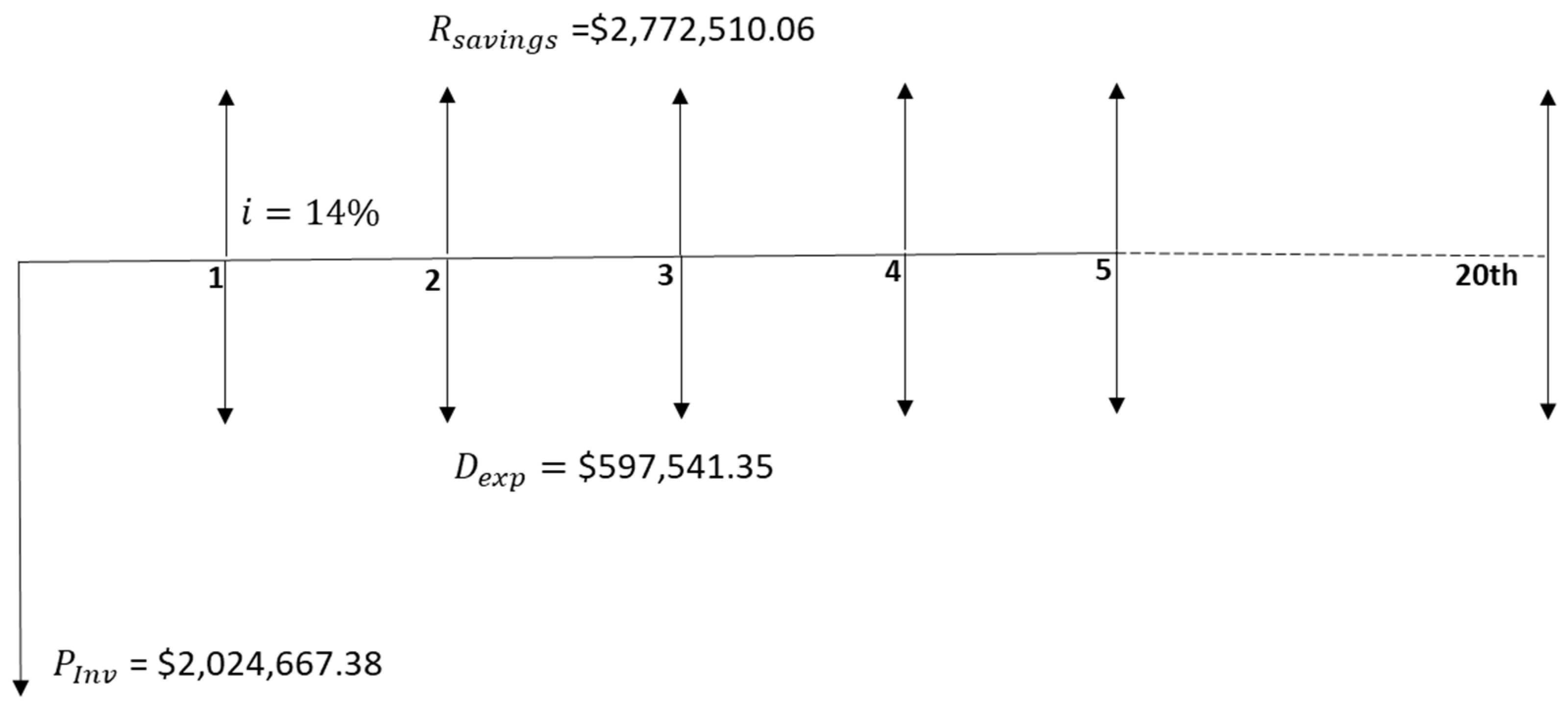
5.3. Results and Analysis on the Farm Energy Audit and Investment Analysis

Results of the energy audit indicate that the farm consumes a total of 11,891,540 MJ of energy per month at a huge cost of USD 0.24 million, adding up to USD 2.93 million per year, as indicated in

Table 6. Results of the energy audit of Songhai Farm.

Fuel	Heat Values (MJ/kg or m3)	Energy/Month (MJ)	Cost/Month ($)	Cost/Year ($M)
Coal	25–35	1,750,000	37,000	0.444
Fuelwood	18.60	651,000	13,000	0.156
Diesel	46.00	2,760,000	64,000	0.768
PMS	46.80	2,808,000	47,400	0.5688
Kerosene	46.26	2,081,700	68,850	0.8262
Biogas	35.8	1,840,750	12,854.4	0.1543
Total		11,891,540	243,104	2.92

. The table shows the monthly quantity of fuel, energy heating values, unit price of fuel, cost of fuel per month, amount of energy consumed per month, and unit costs for each energy source utilized. As previously mentioned, the farm does not have reliable power from the electricity grid, and as such, the energy audit highlights the need for a cost-effective, affordable, and low-carbon energy MES integrated with a P2G unit for optimal energy conversion and supply.

The NPV analysis consists of two parts, including the NPV of unpriced saving (benefit) investments. In this paper, the annual savings are the difference between the farm’s total annual cost using current fossil-based fuels and the MES’s total annual cost. Here, all the unpriced benefits of investing in the MES for the period of twenty years are taken into consideration. These unpriced benefits include the afforestation of the once deforested environment due to fuelwood exploitation, sanitation as a result of converting organic waste into the production of biomethane, clean air, good health for humans and animals, and development.

The investment analysis considers the cost of fuel utilized by the farms, the investment (capital + replacement + maintenance), operations, emissions and energy not supplied (ENS) costs of the MES, the MES’s lifespan, and the cost savings in the purchase of fuelwood, kerosene, PMS, diesel, biogas, coal, and labour by the farm as shown in

Table 7. Net present cost (NPC) analysis for the MES.

Type of Cost		Year 1	Years 2–20 (Per Year)
Farm Annual Costs	Fuel	2,771,400	2,771,400
	Labour	560.06	560.06
	O&M	550	550
	Total Annual	2,772,510.06	2,772,510.06
	Present Worth	18,355,259.34	-
MES Costs	Investment	2,024,667.38	-
	Operations	566,741.37	566,741.37
	Emissions	30,799.98	30,799.98
	Total Annual	2,622,208.73	597,541.35
	Present Worth	5,982,243.50	-
Net Benefit		150,301.33	2,174,968.71

.

Based on calculations, the total yearly cost avoided or saved, $R_{savings}$, amounts to USD 2.772 million, with an investment cost $P_{Inv}$ of USD 2.025 million. The total yearly expenses, $D_{exp}$, are USD 597,541.35, and there is a net present value (NPV) of USD 12.37 million. The benefit–cost ratio (BCR) is 2.3. The internal rate of return (IRR) exceeds 60%, and the profitability index (PI) stands at 7.12. The cost payback period is 2.75 years (2 years and 9 months). An assumed interest rate of 14% is applied, and the project is expected to have a lifespan of twenty (20) years with no salvage value. The operational lifespan of the facility is set at twenty (20) years, primarily due to the negligible significance of any costs incurred beyond this period when discounted to the present value. Savings denote the monetary value of costs avoided or preserved through the ownership of an MES. For example, a farm that previously spent USD 826,200 annually on purchasing kerosene for cooking now saves that amount by switching to using an MES to meet its energy needs, eliminating the need to buy kerosene and other fuels.

The investment indices and decisions for the MES project in the case study farm are shown in

Table 8. Investment/economic indices of the MES.

Investment Indices	Values	Indication
NPC/NPV	USD 12.37 million	viable
BCR	2.3	viable
IRR	Above 60%	acceptable
PI	7.12	viable

. Figure 4 shows the cash flow diagram of the MES investment.

Accordingly, the investment in the MES is projected to yield cumulative annual savings of approximately 2.772 million over its expected 20-year operational lifespan. With a net present value of USD 12.37 million, a benefit–cost ratio of 2.3, and an internal rate of return of over 60%, the investment analysis indicates an annual saving of USD 2.77 million for the farm upon integrating the proposed MES as its energy source. These findings suggest that Scenario 4 presents the most optimal planning costs, while the investment analysis underscores the economic viability of adopting an MES in the farm.

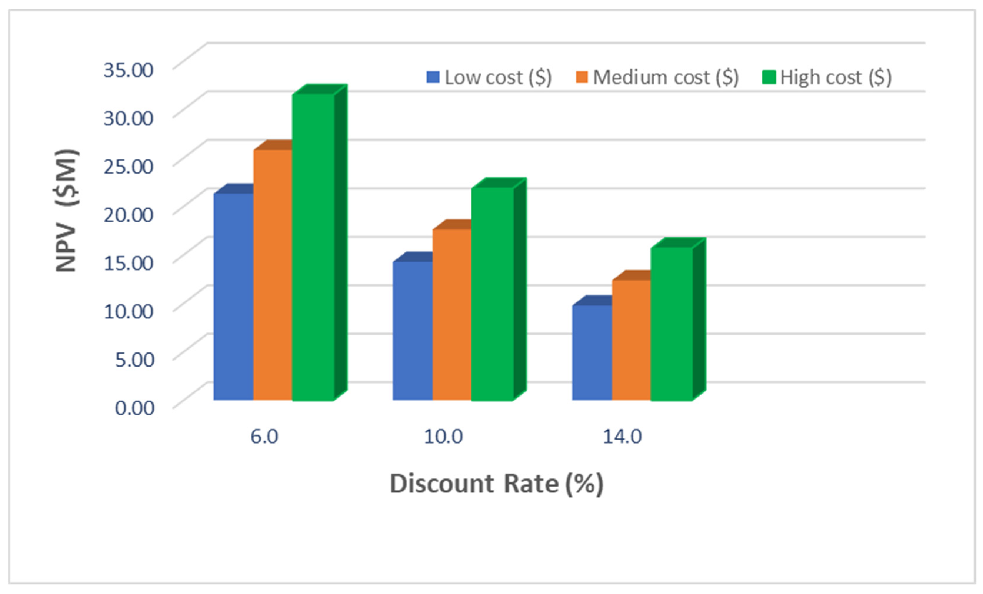
5.4. Sensitivity Analysis on the Discount Rate and Fuel Price

Sensitivity analysis is used to determine how the investment measures, such as the NPV, PW, BCR, IRR, and PI, change when one or more input parameters such as fuel cost and/or discounting rate vary over a selected range of values. The MES investment sensitivity analysis examines the economic advantages among the three alternatives by making three estimates for each category of fuel cost: a low-cost, medium-cost, and high-cost estimate. This approach allows us to study measures of worth and alternative selection sensitivity within a predicted range of variation for each parameter depending on implement conditions.

Table 9. Three different unit prices of fuel consumed by the farm.

Fuel Source	Quantity/ Month	Unit Price ($) Low	Unit Price ($) Medium	Unit Price ($) High
Coal	50,000 kg	0.78	0.74	0.85
Fuelwood	35,000 kg	0.50	0.45	0.55
Diesel	60,000 L	0.85	1.07	1.25
PMS	60,000 L	0.58	0.79	1.02
Kerosene	45,000 L	1.26	1.53	1.65
Biogas	51,417.6 m3	0.25	0.25	0.25

shows the unit price of three categories of fuel consumed by the farm.

As indicated in

Table 10. Energy audit for three different yearly costs of fuel consumed by the farm.

Fuel	Heat Values (MJ/kg or m3)	Energy/Month (MJ)	Cost/Year Low ($M)	Cost/Year Medium ($M)	Cost/Year High ($M)
Coal	25-35	1,750,000	0.468	0.444	0.510
Fuelwood	18.60	651,000	0.210	0.162	0.231
Diesel	46.00	2,760,000	0.612	0.7704	0.9
PMS	46.80	2,808,000	0.408	0.5688	0.734
Kerosene	46.26	2,081,700	0.680	0.8262	0.891
Biogas	35.8	1,840,750	0.1543	0.1543	0.1543
Total		11,891,540	2.53	2.92	3.42

, the calculated total annual fuel costs for the low-, medium-, and high-cost estimates stand at 2.53, 2.92, and 3.42, respectively.

Figure 5 shows the relationship between NPV and discounting rate for the three fuel cost categories and three discount rates in the sensitivity analysis. As seen, though all three fuel cost zones give satisfactory measures of worth for the MES investment, the NPVs are higher at a discount rate of 6%, suggesting that a lower MARR is favourable for the MES investment than higher discount rates.

Further information about the summary of the NPV sensitivity analysis for low, medium, and high fuel costs is presented in

Table A6. Summary of the NPV sensitivity analysis for low, medium, and high fuel costs.

Costs ($)		Year 1	Year 2…20	Discount Rate (%)
Low cost		2,378,000	2,378,000	$i=6$
Farm total cost		2,379,110.06	2,379,110.06
Present worth	27,288,154.48
MES total cost		2,369,681.31	345,013.93
Present Worth	5,981,942.66
Net Benefit		9428.75	2,034,096.13
Investment Indices: NPV = 21,306,212.82, IRR = Above 60%, BCR = 4.6, PI = 11.52
Low cost		2,378,000	2,378,000	$i=10$
Farm total cost		2,379,110.06	2,379,110.06
Present worth	20,254,791.41
MES total cost		2,489,514.1	464,846.72
Present Worth	5,982,186.42
Net Benefit		−110,404.04	1,914,263.34
Investment Indices: NPV = 14,272,605.99, IRR = Above 60%, BCR = 3.4, PI = 8.01
Low cost		2,378,000	2,378,000	$i=14$
Farm total cost		2,379,110.06	2,379,110.06
Present worth	15,757,083.84
MES total cost		2,622,208.73	597,541.35
Present Worth	5,982,243.50
Net Benefit		−243,098.67	1,781,568.71
Investment Indices: NPV = 9,774,840.34, IRR = Above 60%, BCR = 2.6, PI = 5.83
Medium cost		2,771,400	2,771,400	$i=6$
Farm toral cost		2,772,510.06	2,772,510.06
Present Worth	31,800,413.14
MES total cost		2,369,681.31	345,013.93
Present Worth	5,981,942.66
Net Benefit		402,828.75	2,427,496.13
Investment Indices: NPV = 25,818,470.48, IRR = Above 60%, BCR = 5.3, PI = 13.7
Medium cost		2,771,400	2,771,400	$i=10$
Farm total cost		2,772,510.06	2,772,510.06
Present Worth	23,604,041.65
MES total cost		2,489,514.1	464,846.72
Present Worth	5,982,186.42
Net Benefit		282,995.96	2,307,663.34
Investment Indices: NPV = 17,621,855.23, IRR = Above 60%, BCR = 3.95, PI = 9.7
Medium cost		2,771,400	2,771,400	$i=14$
Farm total cost		2,772,510.06	2,772,510.06
Present Worth	18,355,259.34
MES total cost		2,622,208.73	597,541.35
Present Worth	5,982,243.50
Net Benefit		150,301.33	2,174,968.71
Investment Indices: NPV = 12,373,016.84, IRR = Above 60%, BCR = 2.3, PI = 7.12
High cost		3,266,000	3,266,000	$i=6$
Farm total cost		3,267,110.06	3,267,110.06
Present Worth	37,473,425.68
MES total cost		2,369,681.31	345,013.93
Present Worth	5,981,942.66
Net Benefit		897,428.73	2,922,096.13
Investment Indices: NPV = 31,491,483.02, IRR = Above 60%, BCR = 6.3, PI = 17.5
High cost		3,266,000	3,266,000	$i=10$
Farm total cost		2,369,681.31	2,369,681.31
Present Worth	27,8148,68.21
MES total cost		2,489,514.1	464,846.72
Present Worth	5,982,186.42
Net Benefit		777,595.96	2,802,263.34
Investment Indices: NPV = 21,832,682.79, IRR = Above 60%, BCR = 4.6, PI = 11.8
High cost		3,266,000	3,266,000	$i=14$
Farm total cost		2,369,681.31	2,369,681.31
Present Worth	21,638,396.64
MES total cost		2,622,208.73	597,541.35
Present Worth	5,982,243.50
Net Benefit		644,901.33	2,669,568.71
Investment Indices: NPV = 15,656,153.14, IRR = Above 60%, BCR = 3.6, PI = 8.7

in Appendix A, which shows that the calculated NPV for the high cost at a discount rate of 6% gives the largest value of USD 31.49 million. This makes it the highest return for the MES investment. Again, the NPV decreases as the discounting rate $i$ is increased from 6% to 10% and 14% in each of the fuel cost categories, low, medium, and high.

Based on the BCR, the high cost at a discount rate of 6% gives the highest BCR of 6.3, which aligns with the NPV analysis. The BCR and the NPV decrease as the discounting factor increases in each fuel cost category. The IRR is greater than the Minimum Acceptable Rate of Return (MARR) in all three fuel cost categories and at all three discounting rates, though to varying degrees. The highest PI value is recorded in the high-cost category at a discounting rate of 6%. The PI value also decreases with an increase in the discounting rate. This study indicates that investment is most favourable with a lower MARR than with a higher rate of return.

6. Conclusions and Recommendations

Motivated by the urgent need to enhance energy sustainability, this paper introduces a planning model that compares the optimal planning costs of a proposed MES across four scenarios and a detailed sensitivity analysis. It includes an investment model to assess the feasibility and viability of implementing the best optimally planned MES as an economical and efficient replacement for the conventional energy source on a case study farm. The numerical results indicate an annual saving of USD 2.77 million for the farm upon integrating the proposed MES and suggest that Scenario 4 with P2G and DRPs presents the most optimal planning costs, and adopting an MES is a feasible investment for the farm.

The MES planning and investment model developed in this paper can be applied to other settings, such as residential areas, industrial complexes, a university campus, etc., by tailoring the data of those settings to the models related to energy demand and supplies for the specific areas of application. Identifying efficient and practical solutions for P2G-integrated multi-energy systems will bring significant advantages, enabling the reliable and renewable supply of electricity, heat, and gas. This contributes to reducing dependence on fossil fuels, lowering carbon emissions, and enhancing overall sustainability in the energy sector.

The availability of MESs is generally increasing and maturing, but it varies by component, integration level, and region. While urban areas often have better infrastructure for integrated systems and digitalization, rural areas lack electrical grid flexibility or heating networks. In developing regions, MES investment faces compounded barriers: technologies are scarce and costly, regulatory frameworks are poorly aligned with system integration, and capital is limited or risk-averse. Also, access to advanced MES technologies is limited due to reliance on costly imports, a shortage of skilled personnel, underdeveloped supply chains, and inadequate digital infrastructure. Additionally, energy governance is often fragmented, with outdated regulations and a lack of integrated planning, thereby discouraging innovation and long-term investment. Financially, high interest rates, limited access to capital, and perceived political and economic risks hinder project financing, while governments struggle to allocate resources. These challenges underscore the need for targeted policy support, capacity building, and blended finance mechanisms to enable MESs as part of a sustainable, resilient energy transition.

To strengthen the applicability of the model, future research should incorporate diverse use cases across different sectors, such as commercial, transport, industrial, residential, and geographic regions. In addition, this work considers the optimal planning of MESs in a deterministic case. The integration of RES in MES planning with the consideration of uncertainties associated with RES, energy demand, and the price of electricity is recommended for future study. These uncertainties can be modelled using the stochastic or probabilistic approach in analyzing the models to account for variabilities and the unpredictability inherent in real-world scenarios. The precise and efficient modelling of these uncertainties is crucial for achieving the optimal integration of renewable energy within the MES.

References

1. Mancarella, P. MES (multi-energy systems): An overview of concepts and evaluation models. Energy 2014, 65, 1–17. [Google Scholar] [CrossRef]
2. Mancarella, P.; Andersson, G.; Peças-Lopes, J.A.; Bell, K.R.W. Modelling of integrated multi-energy systems: Drivers, requirements, and opportunities. In Proceedings of the 2016 Power Systems Computation Conference (PSCC), Genoa, Italy, 20–24 June 2016; pp. 1–22. [Google Scholar]
3. Ademollo, A.; Carcasci, C.; Ilo, A. Behavior of the Electricity and Gas Grids When Injecting Synthetic Natural Gas Produced with Electricity Surplus of Rooftop PVs. Sustainability 2024, 16, 9747. [Google Scholar] [CrossRef]
4. Shobayo, L.O.; Dao, C.D. Smart Integration of Renewable Energy Sources Employing Setpoint Frequency Control—An Analysis on the Grid Cost of Balancing. Sustainability 2024, 16, 9906. [Google Scholar] [CrossRef]
5. Alabi, T.M.; Agbajor, F.D.; Yang, Z.; Lu, L.; Ogungbile, A.J. Strategic potential of multi-energy system towards carbon neutrality: A forward-looking overview. Energy Built Environ. 2023, 4, 689–708. [Google Scholar] [CrossRef]
6. Ma, T.; Wu, J.; Hao, L.; Lee, W.-J.; Yan, H.; Li, D. The optimal structure planning and energy management strategies of smart multi energy systems. Energy 2018, 160, 122–141. [Google Scholar] [CrossRef]
7. Onen, P.S.; Mokryani, G.; Zubo, R.H.A. Planning of Multi-Vector Energy Systems with High Penetration of Renewable Energy Source: A Comprehensive Review. Energies 2022, 15, 5717. [Google Scholar] [CrossRef]
8. Wang, J.; Hu, Z.; Xie, S. Expansion planning model of multi-energy system with the integration of active distribution network. Appl. Energy 2019, 253, 113517. [Google Scholar] [CrossRef]
9. Cao, J.; Crozier, C.; McCulloch, M.; Fan, Z. Optimal Design and Operation of a Low Carbon Community Based Multi-Energy Systems Considering EV Integration. IEEE Trans. Sustain. Energy 2019, 10, 1217–1226. [Google Scholar] [CrossRef]
10. Son, Y.-G.; Oh, B.-C.; Acquah, M.A.; Fan, R.; Kim, D.-M.; Kim, S.-Y. Multi Energy System With an Associated Energy Hub: A Review. IEEE Access 2021, 9, 127753–127766. [Google Scholar] [CrossRef]
11. Sokolnikova, P.; Lombardi, P.; Arendarski, B.; Suslov, K.; Pantaleo, A.M.; Kranhold, M.; Komarnicki, P. Net-zero multi-energy systems for Siberian rural communities: A methodology to size thermal and electric storage units. Renew. Energy 2020, 155, 979–989. [Google Scholar] [CrossRef]
12. Geidl, M.; Koeppel, G.; Favre-Perrod, P.; Klockl, B.; Andersson, G.; Frohlich, K. Energy hubs for the future. IEEE Power Energy Mag. 2007, 5, 24–30. [Google Scholar] [CrossRef]
13. Pazouki, S.; Haghifam, M.-R. Optimal planning and scheduling of energy hub in presence of wind, storage and demand response under uncertainty. Int. J. Electr. Power Energy Syst. 2016, 80, 219–239. [Google Scholar] [CrossRef]
14. Noorollahi, Y.; Golshanfard, A.; Hashemi-Dezaki, H. A scenario-based approach for optimal operation of energy hub under different schemes and structures. Energy 2022, 251, 123740. [Google Scholar] [CrossRef]
15. Chen, X.; Cao, W.; Xing, L. GA Optimization Method for a Multi-Vector Energy System Incorporating Wind, Hydrogen, and Fuel Cells for Rural Village Applications. Appl. Sci. 2019, 9, 3554. [Google Scholar] [CrossRef]
16. Eladl, A.A.; El-Afifi, M.I.; El-Saadawi, M.M.; Sedhom, B.E. A review on energy hubs: Models, methods, classification, applications, and future trends. Alex. Eng. J. 2023, 68, 315–342. [Google Scholar] [CrossRef]
17. Mazza, A.; Bompard, E.; Chicco, G. Applications of power to gas technologies in emerging electrical systems. Renew. Sustain. Energy Rev. 2018, 92, 794–806. [Google Scholar] [CrossRef]
18. Qin, G.; Yan, Q.; Kammen, D.M.; Shi, C.; Xu, C. Robust optimal dispatching of integrated electricity and gas system considering refined power-to-gas model under the dual carbon target. J. Clean. Prod. 2022, 371, 133451. [Google Scholar] [CrossRef]
19. Onen, P.S.; Zubo, R.H.A.; Mokryani, G.; Abd-Alhameed, R. A Bi-Level Bidding Strategy Model for Gas-Fired units, Power-to-Gas facility and Renewable Power in a coordinated Energy Market Considering Demand Response Programs. 2023. Available online: https://ssrn.com/abstract=4602639 (accessed on 18 January 2025).
20. Jiang, J.; Zhang, L.; Wen, X.; Valipour, E.; Nojavan, S. Risk-based performance of power-to-gas storage technology integrated with energy hub system regarding downside risk constrained approach. Int. J. Hydrogen Energy 2022, 47, 39429–39442. [Google Scholar] [CrossRef]
21. Habibifar, R.; Khoshjahan, M.; Ghasemi, M.A. Optimal Scheduling of Multi-Carrier Energy System Based on Energy Hub Concept Considering Power-to-Gas Storage. In Proceedings of the 2020 IEEE Power & Energy Society Innovative Smart Grid Technologies Conference (ISGT), Washington, DC, USA, 17–20 February 2020; pp. 1–5. [Google Scholar]
22. Eladl, A.A.; El-Afifi, M.I.; Saeed, M.A.; El-Saadawi, M.M. Optimal operation of energy hubs integrated with renewable energy sources and storage devices considering CO2 emissions. Int. J. Electr. Power Energy Syst. 2020, 117, 105719. [Google Scholar] [CrossRef]
23. Sun, H.; Sun, X.; Kou, L.; Ke, W. Low-Carbon Economic Operation Optimization of Park-Level Integrated Energy Systems with Flexible Loads and P2G under the Carbon Trading Mechanism. Sustainability 2023, 15, 15203. [Google Scholar] [CrossRef]
24. Zhang, S.; Pan, G.; Li, B.; Gu, W.; Fu, J.; Sun, Y. Multi-Timescale Security Evaluation and Regulation of Integrated Electricity and Heating System. IEEE Trans. Smart Grid 2025, 16, 1088–1099. [Google Scholar] [CrossRef]
25. Yang, C.; Dong, X.; Wang, G.; Lv, D.; Gu, R.; Lei, Y. Low-carbon economic dispatch of integrated energy system with CCS-P2G-CHP. Energy Rep. 2024, 12, 42–51. [Google Scholar] [CrossRef]
26. Alizad, E.; Rastegar, H.; Hasanzad, F. Dynamic planning of Power-to-Gas integrated energy hub considering demand response programs and future market conditions. Int. J. Electr. Power Energy Syst. 2022, 143, 108503. [Google Scholar] [CrossRef]
27. Thommessen, C.; Otto, M.; Nigbur, F.; Roes, J.; Heinzel, A. Techno-economic system analysis of an offshore energy hub with an outlook on electrofuel applications. Smart Energy 2021, 3, 100027. [Google Scholar] [CrossRef]
28. Xia, Q.; Zou, Y.; Wang, Q. Optimal Capacity Planning of Green Electricity-Based Industrial Electricity-Hydrogen Multi-Energy System Considering Variable Unit Cost Sequence. Sustainability 2024, 16, 3684. [Google Scholar] [CrossRef]
29. Chambon, C.L.; Karia, T.; Sandwell, P.; Hallett, J.P. Techno-economic assessment of biomass gasification-based mini-grids for productive energy applications: The case of rural India. Renew. Energy 2020, 154, 432–444. [Google Scholar] [CrossRef]
30. Di Micco, S.; Romano, F.; Jannelli, E.; Perna, A.; Minutillo, M. Techno-economic analysis of a multi-energy system for the co-production of green hydrogen, renewable electricity and heat. Int. J. Hydrogen Energy 2023, 48, 31457–31467. [Google Scholar] [CrossRef]
31. Oyaniran, T. Current State of Nigeria Agriculture and Agribusiness Sector; AfCFTA: Accra, Ghana, 2020. [Google Scholar]
32. He, L.; Lu, Z.; Zhang, J.; Geng, L.; Zhao, H.; Li, X. Low-carbon economic dispatch for electricity and natural gas systems considering carbon capture systems and power-to-gas. Appl. Energy 2018, 224, 357–370. [Google Scholar] [CrossRef]
33. Kenarsari, S.D.; Yang, D.; Jiang, G.; Zhang, S.; Wang, J.; Russell, A.G.; Wei, Q.; Fan, M. Review of recent advances in carbon dioxide separation and capture. RSC Adv. 2013, 3, 22739–22773. [Google Scholar] [CrossRef]
34. Majidi, M.; Nojavan, S.; Zare, K. A cost-emission framework for hub energy system under demand response program. Energy 2017, 134, 157–166. [Google Scholar] [CrossRef]
35. Futo, S. Challenges and Prospects of Grasscutter Farming in Selected Areas of Rivers State, Nigeria. Int. J. Agric. Rural. Dev. 2016, 19, 2600–2610. [Google Scholar]
36. Mtamabari, T.; Ebigennibo, S. Economics of Methane Production from Animal Dung Using 681.3 M3 Fixed-Domes Digester for Farm Application. Afr. J. Eng. Environ. Res. 2021, 9, 146–162. [Google Scholar]
37. Nigeria Central Bank. Nigeria Interest Rate. Available online: https://tradingeconomics.com/nigeria/interest-rate (accessed on 25 May 2025).
38. GAMS. GAMS The Modelling Language. Available online: https://www.gams.com/products/gams/gams-language/ (accessed on 28 April 2025).
Figure 1. Proposed model of the P2G-MES.
Sustainability 17 05759 g001
Figure 2. The configuration of a power-to-gas unit.
Sustainability 17 05759 g002
Figure 3. Core elements of the proposed optimal planning and investment model.
Sustainability 17 05759 g003
Figure 4. Cash flow diagram of MES investment.
Sustainability 17 05759 g004
Figure 5. Net present value vs. discounting rate for the sensitivity analysis.
Sustainability 17 05759 g005