Route Optimization of Multimodal Transport Considering Regional Differences under Carbon Tax Policy

Abstract

Environmental sustainability is receiving growing global attention, making the development of low-carbon and green transportation increasingly important. Low-carbon policies offer significant advantages in incentivizing energy conservation and reducing emissions in the transportation sector; however, it is vital to consider the impacts of regional differences on the implementation effect of low-carbon policies. This paper explores multimodal transportation route optimization under a carbon tax policy. First, a bi-objective route optimization model is constructed, with the goal of minimizing total transportation cost and time, while accounting for uncertain demand, fixed departure schedules, and regional differences. Trapezoidal fuzzy numbers are used to represent uncertain demand, and a fuzzy adaptive non-dominated sorting genetic algorithm is designed to solve the bi-objective optimization model. The algorithm is then tested on differently sized networks and on real-world transportation networks in eastern and western China to validate its effectiveness and to assess the impacts of regional differences. The experimental results show the following. (1) When considering transportation tasks at different network scales, the proposed fuzzy adaptive non-dominated sorting genetic algorithm outperforms the NSGA-II algorithm, achieving minimum differences in percentages of cost and time of 9.25% and 7.72%, respectively. (2) For transportation tasks assessed using real-world networks in eastern and western China, an increase in the carbon tax rate significantly affects carbon emissions, costs, and time. The degree of carbon emission reduction varies depending on the development of the regional transportation network. In the more developed eastern region, carbon emissions are reduced by up to 44.17% as the carbon tax rate increases. In the less developed western region, the maximum reduction in carbon emissions is 14.37%. The carbon tax policy has a more limited impact in the western region compared to the eastern one. Therefore, formulating differentiated carbon tax policies based on local conditions is an effective way to maximize the economic and environmental benefits of multimodal transportation.

1. Introduction

Environmental protection has become a central focus of public concern in response to global climate change and ecological environment challenges. The transportation sector is a major carbon emission source, accounting for 24% of global carbon emissions [1]. This highlights the need to promote a low-carbon transition in transportation. Multimodal transport, as one of the most important transportation organizational models, plays a significant role in optimizing transport structures, improving efficiency, and achieving green transportation. This is a key direction for the green transformation of the transportation sector.

Carbon tax policies are a market-based tool for controlling carbon emissions, and have been widely adopted given their ability to incentivize emission reductions through price signals [2]. Most studies on the impact of carbon tax policies on transportation carbon emissions have focused on the national macro level; few studies consider regional differences. However, there are significant disparities in the development of transportation systems across different regions of China. Regional freight transport networks vary in terms of infrastructure, economic conditions, and logistics capabilities. This means that carbon tax policies may have different impacts across regions. This is a research gap, as there is value in applying a regional perspective to examine the differentiated impacts of carbon tax policies on energy-saving and emission-reduction effects in multimodal transportation. This research provides insights for formulating differentiated and precise carbon reduction measures; this is significant for supporting the green transformation of the transportation industry.

The introduction of green and low-carbon development concepts has led people to pay attention to optimizing low-carbon multimodal transportation routes [3,4]. Uncertainty is common in complex transportation environments. These uncertainties include factors such as transportation demand [5,6], transportation time [7,8,9], transportation cost [10], and node capacity [11,12]. Accounting for these uncertainties in low-carbon multimodal route optimization makes such research applicable to real-world scenarios. The low-carbon multimodal transportation route optimization problem under uncertainty is solved by determining the optimal transportation routes and modes for a given logistics task, based on carbon emissions during transport or the specific meaning of low-carbon policies [13].

Past research has primarily focused on developing multimodal transportation route optimization models, with objectives such as minimizing transportation cost and transportation time or maximizing customer satisfaction by meeting demand. These studies generally incorporate carbon emissions into the objective function or set them as a constraint. For instance, Li et al. [14] proposed a multi-objective optimization model under uncertain transportation demand and time, considering total cost, total time, and carbon emissions. Ziaei et al. [15] focused on hazardous materials transportation, developing an optimization model focused on minimizing carbon emissions, transportation risk, and cost, and considering multiple uncertain factors. Through real-world case studies, they explored the relationship between cost, carbon emissions, and transportation risk. Huang et al. [16] incorporated uncertainty in node loads and constructed an optimization model with the objectives of lowering cost and carbon emissions and increasing customer satisfaction. This was solved using a cooperative co-evolutionary algorithm. Zhang et al. [17] considered uncertain demand and time windows, and introduced total carbon emissions as a constraint to limit emissions during transportation.

Other studies have focused on translating carbon emissions into carbon emission costs through low-carbon policies to analyze their impact on transportation plans, or they have compared the emission reduction effects of different low-carbon policies. For example, Zhang et al. [18] examined carbon tax policies, studying the green multimodal transportation route optimization problem under conditions where transportation time follows a random distribution and changes dynamically. They explored the impacts of different transportation time scenarios and carbon tax rates on transportation plans. Sun et al. [19] developed a fuzzy nonlinear optimization model, with the goal of minimizing cost given uncertainties in capacity and carbon trading prices; they also used real-world cases to examine the influence of carbon trading policies on transportation planning. Liu et al. [20] applied the carbon tax policy framework to develop a route optimization model for cold chain containerized multimodal transport, with the goal of minimizing cost. The study incorporated the influence of time-varying networks, and analyzed both dynamic and static optimization scenarios to explore their effects on transportation-related carbon emissions.

Zhang et al. [21] constructed a route optimization model considering both cost and time under uncertain transportation demand and transportation time. They analyzed the effects of carbon tax, carbon trading, carbon offset, and mandatory emission reduction policies on total transportation cost and carbon emissions. Wu et al. [22] developed an optimization model for the transportation of oversized and heavy cargo to minimize cost, and designed various carbon pricing strategies. Using a practical case analysis, they compared the impacts of different carbon tax rates and carbon trading prices on transportation plans, and explored the differences in emission reduction effects between carbon tax and carbon trading policies. Zhu et al. [23] built a multi-objective route decision-making model under different carbon policies, considering the uncertainties in road transport speed and transfer time. They also discussed how these uncertainties, combined with carbon emission policies, influence routing decisions. These studies have been useful; yet, few studies have considered regional differences when examining the energy-saving and emission-reduction effects of low-carbon policies and their impact on transportation planning.

In summary, to address research gaps, this study takes the carbon tax policy as the background, and considers uncertain demand, fixed departure schedule constraints, and regional differences. A dual-objective path optimization model is constructed with the minimum total transportation cost and time. Uncertainty is addressed using trapezoidal fuzzy numbers and the fuzzy chance constraint planning method. A fuzzy adaptive non-dominated sorting genetic algorithm is developed to solve the model. The effectiveness of the model and algorithm is assessed using randomized test cases, and the impact of regional differences on the emission reduction effectiveness of carbon tax policy is further examined using real-world case studies. The findings provide valuable insights for designing low-carbon policies and decision-making in freight transportation enterprises.

2. Problem Description and Model Formulation

2.1. Problem Description

In a multimodal transport network system, a cargo carrier plans to transport a shipment from origin city O to destination city D. During transportation, the cargo passes through nodes; adjacent nodes can be connected by three modes of transport—highway, railway, and waterway. If the transportation mode needs to change at an intermediate node, and the next mode selected is either railway or waterway, waiting times and storage costs may arise due to fixed departure schedules for railway and waterway transport. The costs, time, and carbon emissions associated with mode transfers at transshipment nodes and transportation between adjacent nodes vary across the network. As a result, the cargo carrier faces the challenge of selecting appropriate transport routes and modes. Different choices lead to variations in total transportation cost, time, and carbon emissions. Figure 1 shows a schematic diagram of the multimodal transport system.

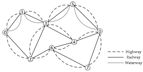
Figure 1. Schematic diagram of the multimodal transportation network.

Moreover, freight demand fluctuates due to the influence of factors such as economic conditions, market dynamics, and policy changes. Therefore, the purpose of this paper is to determine the optimal mode and route of transportation for cargo when specific cargo demand cannot be determined. It comprehensively considers transportation cost, transshipment cost, storage cost, and carbon emission cost throughout the multimodal transport process. Under the constraint of fixed departure schedules, the total transportation cost and time are set as optimization objectives. The ultimate goal is to provide the carrier with an economically viable, time-efficient, and environmentally friendly reference solution based on certain conditions.

The impact of fixed departure schedules on vehicle transshipment scheduling is illustrated in Figure 2. The figure shows that if the subsequent mode of transport is rail or waterway, the cargo arriving at the transshipment node at time T₁ must first undergo necessary transshipment operations. These are completed by time T₂. However, due to the fixed departure schedules of rail and waterway transport, the vehicle must wait until the next scheduled departure at time T₃ to continue the journey. This results in a waiting time window between T₂ and T₃. In contrast, if the subsequent mode is road transport, the cargo can depart immediately after completing transshipment at time T₂. This avoids a schedule-related delay, as road transport is not constrained by fixed departure times.

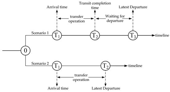
Figure 2. Transit node operation time window.

2.2. Problem Assumptions

This paper makes the following assumptions [24,25,26] to facilitate the modeling solution:

• The same cargo batch is inseparable in transportation;
• Cargo transshipment can only occur at nodes, and a node can only be transshipped once;
• The cargo arrival time is the start time of transshipment;
• After completing transit, the cargo can only be shipped to the next node by selecting the nearest departure time;
• There is an adequate capacity of transportation and transshipment facilities.

2.3. Description of Symbols and Variables

The multimodal transportation network is represented by $G=(N,A,M)$ and $N,A,M$ for the set of nodes (N), the set of arcs (A), and the set of modes of transportation (M). In this expression, $N=\{i|i=1,2\dots ,n\}$, $A=\{a_{ij}|i,j\in N\}$ and $M=\{k|k=1,2\dots ,m\}$. Model parameters and symbols are shown in Table 1.

Table 1. Meanings of model parameters and variables.

Parameter	Description
$C$	Total transportation cost
$T$	Total transportation time from origin to destination
$E$	Total carbon emission
$\tilde{q}$	Fuzzy demand
$c^k$	Unit transportation cost for mode $k$
$c_i^{kl}$	Unit transit cost of switching transportation mode from $k$ to $l$ at node $i$
$c_s$	Storage cost per unit of cargo
$c_p$	Price per unit of carbon emission
$t_{ij}^k$	Transportation time for mode $k$ between transportation nodes $i$ and $j$
$t_i^{kl}$	Transit time per unit to convert transportation mode from $k$ to $l$ at node $i$
$T_i^G$	Time cargo leaves node $i$
$T_i^R$	Time cargo arrives at node $i$
$T_i^{fin}$	Time for cargo to complete transshipment at node $i$
$T_i^w$	Waiting time for cargo at node $i$
${\Gamma }_{ij}^k$	Schedule corresponding to transportation mode $k$ from nodes $i$ and $j$. The schedule is known in advance and ${\Gamma }_{ij}^k=(\cdots {\Phi }_{n-1},{\Phi }_n\cdots ),{\Phi }_n$ denotes the departure time of the $n$ shift
$d_{ij}^k$	Transportation distance between nodes $i$ and $j$ using transportation mode $k$
$v_k$	Average speed of transportation mode $k$
$e^k$	Carbon emission per unit for mode $k$
$e_i^{kl}$	Carbon emission per unit of transit at node $i$ converting transportation mode $k$ to $l$
Variables	Description
$x_{ij}^k$	The value is equal to 1 if transportation mode $k$ is used to transport from node $i$ and $j$. Otherwise, it is equal to 0.
$y_i^{kl}$	The value is equal to 1 if the transportation mode at node $i$ shifts from $k$ to $l$. Otherwise, it is equal to 0.

2.4. Fuzzy Demand Analysis

In transportation, demand for cargo may change based on economic fluctuations, seasonal demand fluctuations, sudden replenishment, and human subjective factors. Therefore, the specific demand for cargo is often uncertain when preparing the transportation plan. Despite this, the cargo carrier can reasonably estimate the approximate range of fluctuations based on historical order data and experience. To address the uncertainty in freight demand, this study adopts a fuzzy programming approach. Previous studies commonly used triangular fuzzy numbers and trapezoidal fuzzy numbers to represent uncertain demand [27]. However, the maximum membership degree of a triangular fuzzy number corresponds to a single point, making it suitable only for well-defined values. In contrast, trapezoidal fuzzy numbers provide greater flexibility, as their maximum membership degree corresponds to an interval. This allows decision-makers to hold differing views on the most likely value. Using trapezoidal fuzzy numbers to represent fuzzy demand is more consistent with real-world conditions. Therefore, this study uses trapezoidal fuzzy numbers to represent the demand as $\tilde{q}=(q^{\min },q^L,q^U,q^{\max })$; this is shown in Figure 3. Here, $u_{\tilde{q}}(q)$ represents the membership function, and $\beta$ denotes the preferred value of the fuzzy demand. Different decision-makers can hold different opinions on the most likely demand interval by adjusting the preference value $\beta$. The result $q^{\min }$ is the most pessimistic estimate, which is unlikely to occur in practice; $[q^L,q^U]$ denotes the upper and lower limits of the most probable demand; and $q^{\max }$ is the most optimistic estimate, which is less likely to occur. These four values are usually determined based on historical transportation data and experience. The affiliation function of fuzzy demand is shown in Equation (1).

$$u(\tilde{q})=\left\{\begin{array}{cc}0,& \tilde{q}\notin [q^{\min },q^{\max }]\\ {\displaystyle \frac{\tilde{q}-q^{\min }}{q^L-q^{\min }}},& \tilde{q}\in [q^{\min },q^L]\\ 1,& \tilde{q}\in [q^L,q^U]\\ {\displaystyle \frac{q^{\max }-\tilde{q}}{q^{\max }-q^U}}& \tilde{q}\in [q^U,q^{\max }]\end{array}\right.$$

(1)

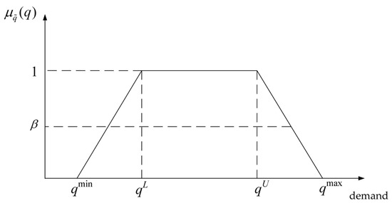
Figure 3. Fuzzy demand.

2.5. Model Building

Objective function:

$$f_1=\min C=\tilde{q}{\displaystyle \sum _{i\in N}{\displaystyle \sum _{j\in N}{\displaystyle \sum _{k\in M}{c}^k}}}{d}_{ij}^k{x}_{ij}^k+\tilde{q}{\displaystyle \sum _{i\in N}{\displaystyle \sum _{k\in M}{\displaystyle \sum _{l\in M}{c}_i^{kl}}}}{y}_i^{kl}+\tilde{q}{\displaystyle \sum _{i\in N}{\displaystyle \sum _{k\in M}{\displaystyle \sum _{l\in M}{c}_s{T}_i^w{y}_i^{kl}}}}+c_{p}E$$

(2)

$$f_2=\min T={\displaystyle \sum _{i\in N}{\displaystyle \sum _{j\in N}{\displaystyle \sum _{k\in M}{t}_{ij}^k}}}{x}_{ij}^k+{\displaystyle \sum _{i\in N\backslash \{o,d\}}{\displaystyle \sum _{k\in M}{\displaystyle \sum _{l\in M}\tilde{q}{t}_i^{kl}}}}{y}_i^{kl}+{\displaystyle \sum _{i\in N\backslash \{o,d\}}{\displaystyle \sum _{k\in M}{\displaystyle \sum _{l\in M}{T}_i^w}}}{y}_i^{kl}$$

(3)

$$T_i^{fin}={\displaystyle \sum _{k\in M}{\displaystyle \sum _{l\in M}(T_i^R}}+\tilde{q}{t}_i^{kl})y_i^{kl},\forall i\in N\backslash \{o\}$$

(4)

$$\phi (T_i^{fin},{\Gamma }_{ij}^k)={\Phi }_n,{\Phi }_{n-1}<T_i^{fin}<{\Phi }_n,\forall k\in M$$

(5)

$$T_i^G={\displaystyle \sum _{l\in M}{\displaystyle \sum _{j\in N\backslash \{o\}}\phi (T_i^{fin}}},{\Gamma }_{ij}^l)x_{ij}^l,\forall i\in N\backslash \{d\}$$

(6)

$$T_j^R={\displaystyle \sum _{k\in M}{\displaystyle \sum _{i\in N\backslash \{d\}}(T_i^G}}+t_{ij}^k)x_{ij}^k,\forall j\in N\backslash \{o\}$$

(7)

$$T_i^w=T_i^G-T_i^{fin},\forall i\in N\backslash (o,d)$$

(8)

$$t_{ij}^k=d_{ij}^k/v_{ij}^k$$

(9)

$$E=\tilde{q}{\displaystyle \sum _{i\in M}{\displaystyle \sum _{j\in N}{\displaystyle \sum _{k\in M}{e}^k}}}{d}_{ij}^k{x}_{ij}^k+\tilde{q}{\displaystyle \sum _{i\in N}{\displaystyle \sum _{k\in M}{\displaystyle \sum _{l\in M}{e}_i^{kl}}}}{y}_i^{kl}$$

(10)

$${\displaystyle \sum _{k\in M}{x}_{ij}^k}\le 1,\forall i,j\in N$$

(11)

$${\displaystyle \sum _{k\in M}{\displaystyle \sum _{l\in M}{y}_i^{kl}\le 1,\forall i\in N}}$$

(12)

$${\displaystyle \sum _{j\in N}{\displaystyle \sum _{k\in M}{x}_{ij}^k}}-{\displaystyle \sum _{j\in N}{\displaystyle \sum _{k\in M}{x}_{ji}^k}}=\left\{\begin{array}{cc}1& i=o\\ -1& i=d\\ 0& i\ne o,d\end{array}\right.$$

(13)

$${\displaystyle \sum _{h\in N}{x}_{hi}^k}+{\displaystyle \sum _{j\in N}{x}_{ij}^l}\ge 2y_i^{kl},\forall i,j,h\in N,k,l\in M$$

(14)

$$x_{ij}^k\in \{0,1\},\forall i,j\in N,k\in M$$

(15)

$$y_i^{kl}\in \{0,1\},\forall i\in N,k,l\in M$$

(16)

Equations (2) and (3) are the objective functions of the model. Equation (2) minimizes the total transportation cost, and consists sequentially of transportation cost, transshipment cost, storage cost, and carbon emission cost. Equation (3) minimizes the total transportation time, and consists sequentially of transportation time, transshipment time, and waiting time. Equations (4)–(15) show the constraints of the model. Equation (4) denotes the moment for the cargo to complete the transshipment at node $i$, where $T_i^R$ denotes the arrival moment of the cargo at node $i$, and $\tilde{q}{t}_i^{kl}$ denotes the time required for the transshipment operation. Equation (5) determines the departure moment of the cargo from node $i$ based on the transshipment completion moment and the departure schedule. If the transshipment is completed after the previous departure moment ${\Phi }_{n-1}$ but before the next scheduled departure moment ${\Phi }_n$, then the departure moment is set to ${\Phi }_n$. Equation (6) establishes the moment that the cargo leaves node $i$. Equation (7) establishes the moment that the cargo arrives at node $j$, where $T_i^G$ denotes the departure moment from the previous node, and $t_{ij}^k$ denotes the transportation time. Equation (8) denotes the waiting time of cargo at node $i$, and is calculated as the actual departure moment from the node minus the moment at which the transshipment operation is completed. Equation (9) denotes the transportation time required between nodes $i$ and $j$ using transportation mode $k$. Equation (10) calculates the carbon emissions during transportation, including both the carbon emissions from transportation between nodes and the carbon emissions from transshipment at hub nodes. Equation (11) establishes that no more than one mode of transportation can be selected between two nodes. Equation (12) establishes that the cargo can change the mode of transportation at node $i$ no more than once. Equation (13) indicates the balance of the node’s cargo flow. Equation (14) denotes the continuity of transportation. Equations (15) and (16) establish that the decision variables are set at 0 or 1.

3. Model Solution

Model Clarity Processing

The objective function of the above model contains fuzzy parameters, which cannot be solved directly using heuristic algorithms. This means the fuzzy variables need to be clarified. This paper draws on the fuzzy chance constraint planning theory proposed by Iwamu-ra and Liu [28]. The original uncertain model is first converted into a fuzzy chance constraint planning model and is then transformed into a deterministic form. The core of this theory is that the decision made ensures that the possibility of satisfying the fuzzy constraints is no less than the given fuzzy preference value. When a number $\alpha$ and a trapezoidal fuzzy number $\tilde{b}=(b_1,b_2,b_3,b_4)$ are provided, fuzzy credibility is used. The fuzzy credibility function is shown in Equation (17). In this expression, $Cr\{\}$ represents the plausibility of the fuzzy event in $\{\}$.

$$Cr\{\tilde{b}\le \alpha \}=\left\{\begin{array}{cc}0,& \alpha \le b_1\\ {\displaystyle \frac{\alpha -b_1}{2(b_2-b_1)}}& b_1\le \alpha \le b_2\\ {\displaystyle \frac{1}{2}},& b_2\le \alpha \le b_3\\ {\displaystyle \frac{a-2b_3+b_4}{2(b_4-b_3)}},& b_3\le \alpha \le b_4\\ 1,& \alpha \ge b_4\end{array}\right.$$

(17)

The fuzzy objective function is clarified based on the above equation. First, the cargo carrier should determine a reasonable fuzzy demand preference value $\beta$ by considering their level of risk preference. In this case, $Cr\{\tilde{b}\le \alpha \}\ge \beta$ holds. From Equation (17), when $\beta \in [0,0.5]$, if $Cr\{\tilde{b}\le \alpha \}\ge \beta$ holds, then $\alpha -b_1\ge 2\beta (b_2-b_1)$. Similarly, when $\beta \in [0.5,1]$, then $\alpha -2b_3+b_4\ge 2\beta (b_4-b_3)$. Based on this, the fuzzy demand $\tilde{q}$ is transformed into a clear value, as shown in Equation (18).

$$\tilde{q}=\left\{\begin{array}{cc}2\beta q^L+(1-2\beta )q^{\min },& 0\le \beta \le 0.5\\ (2-2\beta )q^U+(2\beta -1)q^{\max },& 0.5<\beta \le 1\end{array}\right.$$

(18)

4. Algorithm Design

The traditional NSGA-II algorithm is commonly used to solve multi-objective optimization problems [29,30]. However, it tends to get stuck within a local optima when using fixed crossover probability P_c and mutation probability P_m. This makes it difficult for the algorithm to search for the globally optimal solution. Therefore, this paper integrates the diversity characteristics of Pareto front non-dominated solutions generated by a bi-objective optimization problem to design an improved fuzzy adaptive non-dominated sorting genetic algorithm based on NSGA-II. The improved algorithm based on fuzzy logic adjusts the P_c and P_m by defining rules within the fuzzy system. The fuzzy system is then integrated into the NSGA-II algorithm as a mechanism to dynamically adjust the P_c and P_m in real time. This optimizes algorithm performance.

The flowchart of the fuzzy adaptive non-dominated sorting genetic algorithm is shown in Figure 4. The algorithm has the following seven components.

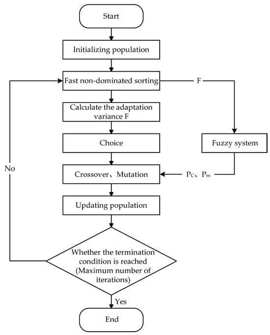
Figure 4. Algorithm flowchart.

• Chromosome coding and decoding

This study uses a two-stage coding method, with a coding length of 2N-1. There are N nodes in the transportation network. Figure 5 shows that for a multimodal transport network with 13 nodes, the corresponding transportation path is 1-2-3-8-9-10-12-13. The transportation modes are waterway–waterway–highway–railway–highway–railway–highway.

Figure 5. Chromosome coding.

2.

Initializing population

The study randomly generates the initial population based on the above encoding rules. First, the starting point of the first encoding segment is set to 1, and the remaining nodes are randomly generated. In the second encoding segment, the transportation mode supported by the corresponding route is randomly selected. This process is repeated NP times to generate an initial population with NP individuals.

3.

Fast Non-dominated Sorting

Non-dominated sorting is performed using pairwise comparisons. Each individual in the population is assigned a rank and a crowding distance. The rank is determined by the number of individuals $n_1$ that individual $i$ dominates and the number $n_2$ of individuals that dominate $i$. The crowding distance is the difference in objective function values between the two individuals adjacent to the specified individual.

4.

Selection of operation

The binary tournament method is used for selection. During selection, two individuals are randomly compared based on their sorting ranks. The individual with the lower rank is selected. If the ranks are equal, the one with the larger crowding distance is selected.

5.

Calculate and normalize the individual fitness variance

Fitness variance is a metric used to measure the variation in fitness among individuals in a population. It reflects the degree of dispersion of fitness across the population and is used to describe the diversity of the population. Fitness variance is calculated as follows:

$$V_d=\sqrt{{\displaystyle \frac{{\displaystyle \sum _{i=1}^n{d}_i^2}}{n}}}$$

(19)

where $d_i$ denotes the deviation of each individual from the mean value $d_i=\sqrt{{(x_i-\stackrel{\_}{x})}^2+{(y_i-\stackrel{\_}{y})}^2}$.

The fitness variance is normalized, as shown in Equation (20).

$$F={\displaystyle \frac{V_d-V_{d\min }}{V_{d\max }-V_{d\min }}}$$

(20)

6.

Adaptive adjustment of $P_c$ and $P_m$

This study adopts a Fuzzy Inference System to adaptively adjust the $P_c$ and $P_m$ [31]. First, the normalized fitness variance $F$ is entered into the fuzzy system, which adaptively adjusts $P_c$ and $P_m$ based on predefined fuzzy rules and the membership functions of $F$, $P_c$, and $P_m$. The membership functions of $F$, $P_c$, and $P_m$ are assumed to be trapezoidal fuzzy numbers. The fuzzy rules are shown in Table 2.

Table 2. Fuzzy rules.

The Fuzzy Values of F	The Fuzzy Values of ${\mathit{P}}_{\mathit{c}}$	The Fuzzy Values of ${\mathit{P}}_{\mathit{m}}$
Large	Large	Small
Medium	Medium	Medium
Small	Small	Large

In this study, the fuzzy values of $F$, $P_c$, and $P_m$ are defined as large, medium, and small; the value range of $P_c$ is set as $P_c\in [0.5,0.97]$, and the value range of $P_m$ is set as $P_m\in [0.03,0.5]$. In the iterative process of the algorithm, a larger value of F indicates there is a higher population diversity. This makes it necessary to increase the $P_c$ and reduce the $P_m$ to more rapidly concentrate the population. When F is smaller, it is necessary to reduce the $P_c$ and increase the $P_m$ to increase the diversity of the solution.

7.

Crossover and mutation

Based on the adaptively adjusted $P_c$ and $P_m$, crossover and mutation operations are applied to individuals in the population to generate new individuals. The crossover operation adopts an improved single-point crossover method, as shown in Figure 6. For the transportation route, identical nodes are selected for crossover, excluding the starting and ending points. If multiple common nodes exist, one is randomly selected as the crossover point. For the transportation mode, the crossover is conducted at the corresponding position based on the selected crossover point in the route. The mutation operation is shown in Figure 7. In the transportation route section, the positions of two nodes are randomly swapped, excluding the starting and ending points. In the transportation mode section, the transportation mode of a route segment is randomly modified.

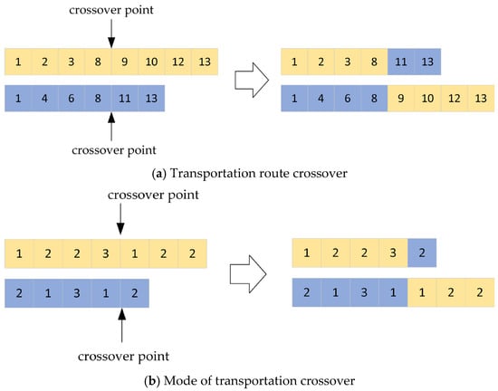
Figure 6. Crossover operation.

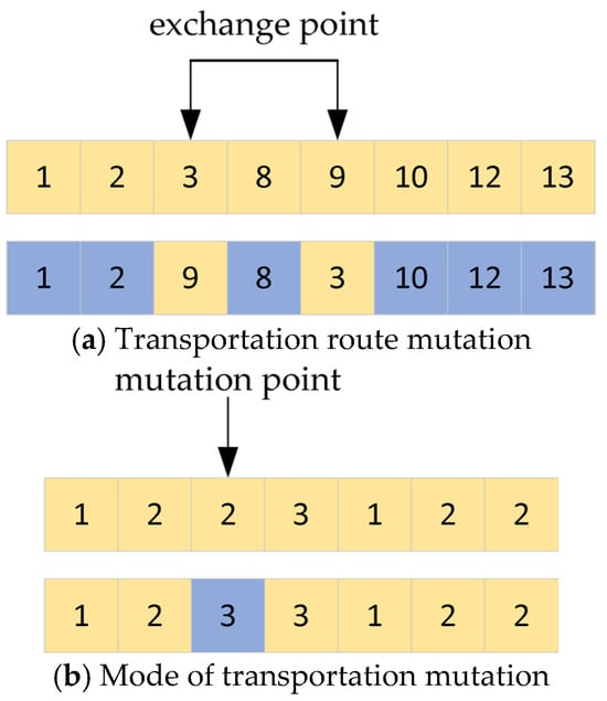
Figure 7. Mutation operation.

5. Case Analysis

5.1. Experimental Environment and Data

The algorithm is implemented using MATLAB 2020a. The algorithm parameters are as follows: the population size is 100; there are 200 iterations; and the initial crossover for P_c is 0.9 and for P_m is 0.1.

In the stochastic example in Section 5.2 and the case study example in Section 5.3, the fuzzy cargo demand is set to $\tilde{q}=(20t,40t,60t,80t)$, and the carbon tax rate is 0.015 RMB/kg. To ensure the reliability of transportation demand and based on relevant literature [14], the fuzzy demand preference value $\beta$ is set to 0.8, and the storage cost for cargo waiting to be dispatched is RMB 8/t.h. The waterway transportation schedule is [00:00, 06:00, 12:00, 18:00], and the railway schedule is [00:00, 03:00, 06:00, 09:00, 12:00, 15:00, 18:00, 21:00]. The highway has no fixed schedule; departures start at 00:00. Parameters in previous studies [32,33] are used as the source for transportation and transshipment parameters for China’s eastern and western regions, as shown in Table 3 and Table 4.

Table 3. Transportation parameters.

Transportation Method	Transportation Speed (km/h)	Unit Transportation Cost (RMB/t.km)	Unit Transportation Carbon Emission (kg/t.km)
Highway	90/90	0.20/0.29	0.071/0.12
Railway	60/60	0.044/0.058	0.042/0.042
Waterway	30/30	0.031	0.012

Table 4. Transit parameters.

Transfer Method	Unit Transit Cost (RMB/t)	Unit Transit Hour (h/t)	Unit Transit Carbon Emission (kg/t)
Highway-Railway	8/10	0.01/0.01	0.128/0.128
Highway-Waterway	9	0.015	0.117
Railway-Waterway	10	0.01	0.113

Note: regarding a/b, a is the parameter for the eastern region and b is the parameter for the western region.

5.2. Algorithm Performance Analysis

Four random test cases with different scales (10, 30, 50, and 100 nodes) are designed to validate the effectiveness of the proposed algorithm. These involved three modes of transportation: highway, railway, and waterway. In the plane coordinate system, the random test cases were generated using specific rules. The representative network diagrams of randomized arithmetic cases are shown in Figure 8 and Figure 9. The transportation and transshipment data for the highway–railway–waterway route are shown in Table 3 and Table 4 for the eastern region.

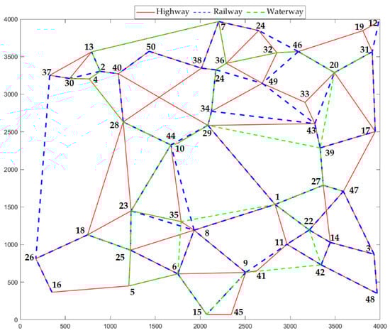
Figure 8. Network diagram for a node size of 50.

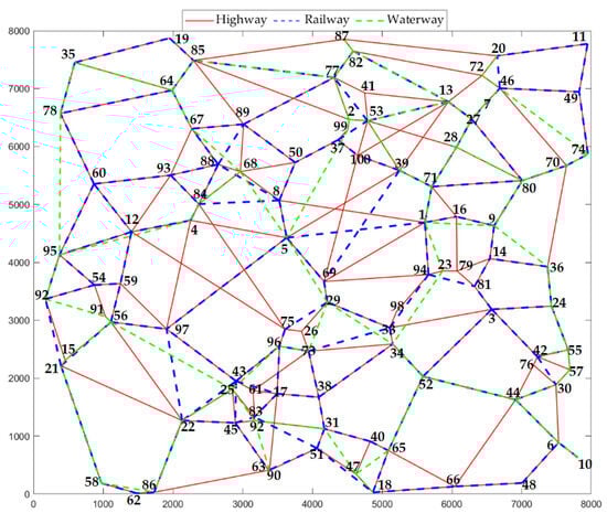
Figure 9. Network diagram for a node size of 100.

Both the fuzzy adaptive non-dominated sorting genetic algorithm designed in this paper and the NSGA-II algorithm were run 20 times on the four differently scaled test cases. Table 5 compares the solution results derived from the two algorithms, where $f_i(i=1,2)$ represents the average value of the objective function. The terms Gap1 and Gap2 indicate the percentage difference between the objective function values obtained by NSGA-II and the fuzzy adaptive non-dominated sorting genetic algorithm, respectively. To ensure a fair comparison, the parameters used in the two tested algorithms matched.

Table 5. Comparison of solution results between NSGA-II algorithm and fuzzy adaptive non-dominated sorting genetic algorithm.

Node Number	Fuzzy Adaptive Undominated Sorting Genetic Algorithm		NSGA-II		Percentage Difference/%
	${\mathit{f}}_1$/103 RMB	${\mathit{f}}_2$/hour	$\mathit{\beta }$/103RMB	${\mathit{f}}_1$/103 RMB	Gap1	Gap2
10	4.70	7.16	4.70	7.16	0	0
30	17.39	57.80	19.00	63.13	9.25	9.22
50	11.62	32.24	12.80	35.82	10.15	11.10
100	31.73	63.18	37.33	68.06	17.65	7.72

Table 5 indicates that the fuzzy adaptive non-dominated sorting genetic algorithm outperforms the NSGA-II algorithm. When there are 10 network nodes, both algorithms generate the same objective values. However, as the number of nodes increases, the objective values obtained by the fuzzy adaptive non-dominated sorting genetic algorithm are consistently better than those generated by the NSGA-II algorithm. The minimum values of Gap1 and Gap2 reach 9.25% and 7.72%, respectively. This shows the fuzzy adaptive non-dominated sorting genetic algorithm has a significant advantage in solving multimodal transportation problems.

5.3. Practical Examples and Analysis

The next research step is constructing a case study based on multimodal transportation in China’s eastern and western regions. In the multimodal transportation network in the eastern region, cargo is transported from Guangzhou to Beijing, passing through Xiamen, Fuzhou, other cities, and Tianjin. Each pair of nodes is connected by three transportation modes: highway, railway, and waterway. In the multimodal transportation network of the western region, cargo is transported from Nanning to Wulumuqi, passing through Baise, Kunming, other cities, and Jiayuguan. Each pair of nodes is connected by two transportation modes: highway and railway. Figure 10 shows the multimodal transportation networks of the two regions. The transportation distances for different modes between cities are in Table 6; they are from the Gaode Map, China Railway Map, and Waterway Network. Other data values are referenced from the experimental data in Section 5.1. The parameter settings for the fuzzy adaptive non-dominated sorting genetic algorithm remain the same as were previously stated.

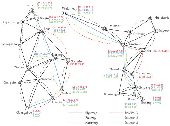
Figure 10. Multimodal transportation network map for eastern and western regions.

Table 6. Transportation distances between nodes in the eastern and western regions.

Eastern Section	Highway (km)	Railway (km)	Waterway (km)	Western Section	Highway (km)	Railway (km)
1–2	635	757	385	1–2	255	223
1–4	675	708	——	1–4	571	482
1–5	781	1049	——	2–3	524	594
2–3	254	226	250	2–4	368	——
2–5	635	773	——	3–4	521	638
3–7	847	937	——	3–5	816	——
3–8	770	883	457	4–5	607	640
4–5	337	342	——	4–6	374	357
4–6	333	406	——	5–6	303	504
5–6	343	362	——	5–7	741	658
5–7	574	587	——	5–9	863	——
6–7	536	512	733	6–7	712	790
6–9	538	536	——	7–8	598	583
6–10	899	1226	——	7–9	646	568
7–8	304	301	376	8–9	1001	——
7–10	617	617	——	8–10	458	612
8–10	822	912	——	9–11	427	468
9–10	467	667	——	9–12	727	770
9–11	417	412	——	9–13	1951	1638
10–11	315	——	——	10–11	680	685
10–12	325	301	——	11–12	942	——
11–12	315	292	——	12–13	1229	1178
11–13	290	266	——
12–13	134	148	——

5.3.1. Case Study Results

This study uses the fuzzy adaptive non-dominated sorting genetic algorithm to obtain the Pareto optimal solution set. Total transportation cost and time are used as evaluation criteria. The entropy weight-TOPSIS method [34] is used to evaluate and rank each solution, thereby identifying the optimal solution.

Table 7 shows the solutions corresponding to the minimum total transportation cost (Solution 1) and the shortest total transportation time (Solution 2) for the eastern and western regions. It also provides the optimal solution (Solution 3) based on the entropy weight-TOPSIS ranking method. Figure 10 shows the transportation route for each solution, along with the arrival and departure times for each node.

Table 7. Case study solution results.

Eastern	Transportation Route	Transportation Mode	Total Cost/RMB	Total Time/Hour
1	1-2-3-8-10-12-13	water-water-water-rail-rail-rail	8338.68	60.18
2	1-2-3-7-10-12-13	road-road-road-road-road-road	40,708.42	31.24
3	1-2-3-7-10-12-13	rail-rail-rail-rail-rail-rail	9595.09	49.77
Western	Transportation Route	Transportation Mode	Total Cost/RMB	Total Time/Hour
1	1-4-6-7-9-13	rail-rail-rail-rail-rail	16,188.92	63.92
2	1-2-4-5-9-13	road-road-road-road-road	84,962.82	44.93
3	1-2-4-5-9-13	road-road-road-road-rail	51,621.90	51.30

Table 7 indicates that the optimal solution for the eastern region has a total transportation cost of RMB 9595.09 and a total transportation time of 49.77 h. For the western region, the optimal solution has a total transportation cost of RMB 51,621.90 and a total transportation time of 51.3 h.

Figure 10 shows that in the eastern region, Solution 1 involves a water-to-rail transshipment at node 8. Due to the fixed departure schedules of rail transport, this results in a total of 2.6 h of transshipment and waiting time; of this total, 1.88 h is waiting time. Solutions 2 and 3 do not involve any transshipment, and do not incur waiting time. In the western region, neither Solutions 1 nor 2 involve transshipment, so there is no waiting time. However, Solution 3 involves a road-to-rail transshipment at node 9, resulting in a total of 0.74 h of transshipment and waiting time; of this total, waiting time accounts for 0.02 h.

5.3.2. Impact Analysis of Carbon Tax Policy

The carbon tax rate affects the selection of transportation routes and modes, impacting total transportation cost, time, and carbon emissions. Carbon tax rates significantly vary across countries. Poland has the lowest carbon tax rate at USD 0.08/t; Sweden has the highest rate at USD 137.24/t [35]. This range is used to evaluate the effects of changes in the carbon tax rate on carbon emissions, costs, and time. To eliminate potential bias with respect to cost and time, the optimal solution based on the entropy weight-TOPSIS method is selected for the carbon tax impact analysis. This study analyzes the impact of the carbon tax rate by comparing the more developed eastern region and the less developed western region of the multimodal transportation network. The results are shown in Figure 11 and Table 8 and Table 9.

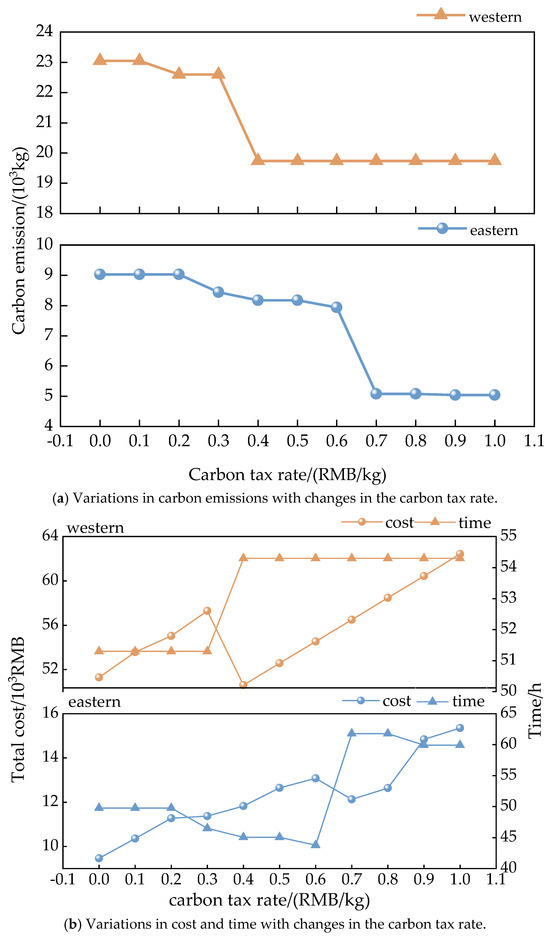
Figure 11. Impact analysis of carbon tax rates.

Table 8. Transportation plans under different carbon tax rates in the eastern region.

Carbon Tax Rate (RMB/kg)	Transportation Route	Transportation Mode
0	1-2-3-7-10-12-13	rail-rail-rail-rail-rail-rail
0.1	1-2-3-7-10-12-13	rail-rail-rail-rail-rail-rail
0.2	1-2-3-7-10-12-13	rail-rail-rail-rail-rail-rail
0.3	1-4-6-10-12-13	rail-rail-rail-rail-rail
0.4	1-5-7-10-12-13	rail-rail-rail-rail-rail
0.5	1-5-7-10-12-13	rail-rail-rail-rail-rail
0.6	1-4-5-6-9-11-13	rail-rail-rail-rail-rail-rail
0.7	1-2-3-8-7-10-12-13	water-water-water-rail-rail-rail-rail
0.8	1-2-3-8-7-10-12-13	water-water-water-rail-rail-rail-rail
0.9	1-2-3-8-10-12-13	water-water-water-rail-rail-road
1.0	1-2-3-8-10-12-13	water-water-water-rail-rail-road

Table 9. Transportation plans under different carbon tax rates in the western region.

Carbon Tax Rate (RMB/kg)	Transportation Route	Transportation Mode
0	1-2-4-5-9-13	road–road-road-road-rail
0.1	1-2-4-5-9-13	road–road-road-road-rail
0.2	1-4-5-9-13	road-road-road-rail
0.3	1-4-5-9-13	road-road-road-rail
0.4	1-4-6-5-9-13	rail–road-road-road-rail
0.5	1-4-6-5-9-13	rail–road-road-road-rail
0.6	1-4-6-5-9-13	rail–road-road-road-rail
0.7	1-4-6-5-9-13	rail–road-road-road-rail
0.8	1-4-6-5-9-13	rail–road-road-road-rail
0.9	1-4-6-5-9-13	rail–road-road-road-rail
1.0	1-4-6-5-9-13	rail–road-road-road-rail

Figure 11a shows that carbon emissions change significantly with different carbon tax rates. In the eastern region, as the carbon tax rate increases, carbon emissions decrease by up to 44.17%. Carbon emissions stabilize after the carbon tax rate reaches 0.7 RMB/kg. In the western region, carbon emissions decrease by up to 14.37% as the carbon tax rate increases. Carbon emissions level off once the carbon tax rate reaches 0.4 RMB/kg.

Figure 11b shows that the total transportation cost increases in a fluctuating upward trend as the carbon tax rate increases. This is because, when the carbon tax rate increases to a certain level, transportation modes tend to shift toward more low-carbon and cost-effective railway and waterway transport. Compared to the higher costs of other modes, this trade-off in transportation efficiency may be acceptable.

Table 8 shows that in the eastern region, a significant structural shift in transportation modes occurs as the carbon tax rates increase. When the carbon tax rate reaches RMB 0.7/kg or higher, the dominant mode gradually shifts from primarily rail transport to lower-carbon modes. These include waterway transport modes, such as rail–water intermodal transport and road–rail–water intermodal transport. This shift is mainly attributed to the developed and well-established inland and coastal waterway networks in the eastern region. These provide low-cost, low-carbon alternatives for cargo transportation.

Table 9 shows that in the western region, the increase in carbon tax rates leads to some route optimization and adjustments in transportation modes. However, fundamental structural shifts in transport methods are difficult to achieve. This is mainly due to geographical constraints and infrastructure limitations in the western region. Examples of these constraints include a lack of waterway transport options and insufficient railway network coverage and connectivity. This prevents a mode transition similar to that in the eastern region.

The changes in carbon emissions and transportation mode show that an increase in the carbon tax rate plays a positive role in reducing carbon emissions. The impact varies depending on the region’s multimodal transportation network. In China’s eastern region, the multimodal transport network is relatively well-developed and includes low-carbon, cost-effective waterway transport options. As such, the carbon tax policy effectively promotes a green transition in transportation modes. As the carbon tax rate rises, carbon emissions decrease significantly; the emissions then stabilize at higher tax levels. In contrast, in the western region, there is a lack of waterway transport and limited railway coverage. This limits the impact of rising carbon tax rates on transportation modes and carbon emissions. Carbon emissions stabilize at lower tax levels; further increases in the tax only increase total transportation costs. Therefore, considering regional differences in the multimodal network, setting an appropriate, regional-focused carbon tax rate is an effective way to improve the environmental and economic benefits of multimodal transportation.

5.3.3. Impact of Fixed Departure Schedules on Transportation Plans Under the Carbon Tax Policy

The constraint of fixed departure schedules affects the cargo carrier’s choice of transportation plans. Different choices lead to variations in transportation cost, time, and carbon emissions. Therefore, this study analyzes the impacts of fixed departure schedules on transportation plans under the carbon tax policy.

According to Table 10 and Table 11, when the carbon tax rate is at a relatively low level, transport schemes without transshipment and schedule constraints demonstrate greater advantages in terms of timeliness and overall cost, as they effectively avoid delays caused by schedule waiting times. However, as the carbon tax rate gradually increases, transport decisions must place greater emphasis on carbon emission costs. Under such circumstances, transport schemes with schedule constraints can optimize routing and scheduling to reduce emissions during transportation, thereby achieving better cost control and greater economic benefits, though this may come at the cost of reduced transport efficiency.

Table 10. Transportation plans and timetables in the eastern region.

Carbon Tax Rate (RMB/kg)	Transportation Route	Transportation Mode	Transportation Schedule (Hour)
0	1-2-3-7-10-12-13	rail-rail-rail-rail-rail- rail	[0.00, 0.00]-[12.62, 12.62]-[16.38, 16.38]-[32.00, 32.00]-42.28, 42.28]-[47.30, 47.30]-[49.77, 49.77]
0.5	1-5-7-10-12-13	rail-rail-rail-rail-rail	[0.00, 0.00]-[17.48, 17.48]-[27.27, 27.27]-[37.55, 37.55]-[42.57, 42.57]-[45.03, 45.03]
1.0	1-2-3-8-10-12-13	water-water-water-rail-rail-road	[0.00, 0.00]-[12.83, 12.83]-[21.17, 21.17]-[36.40, 39.00]-[52.70, 52.70]-[57.72, 58.44]-[59.93, 59.93]

Table 11. Transportation plans and timetables in the western region.

Carbon Tax Rate (RMB/kg)	Transportation Route	Transportation Mode	Transportation Schedule (Hour)
0	1-2-4-5-9-13	road-road-road-road-rail	[0.00, 0.00]-[2.83, 2.83]-[6.92, 6.92]-[13.67, 13.67]-[23.26, 24.00]-[51.3, 51.3]
0.5	1-4-6-5-9-13	rail-road-road-road-rail	[0.00, 0.00]-[8.03, 8.75]-[12.91, 12.91]-[16.28, 16.28]-[25.86, 27.00]
1.0	1-4-6-5-9-13	rail-road-road-road-rail	[0.00, 0.00]-[8.03, 8.75]-[12.91, 12.91]-[16.28, 16.28]-[25.86, 27.00]

5.3.4. Sensitivity Analysis of Fuzzy Demand Preference Values

The size of the fuzzy demand preference value reflects the customer’s preference for transportation reliability. To analyze the impact of the fuzzy demand preference value on total transportation cost and carbon emissions, the study includes a sensitivity analysis of this value. The selected solution is the optimal solution based on the entropy weight-TOPSIS ranking method. The results are shown in Figure 12.

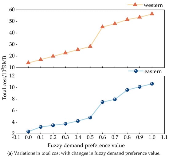
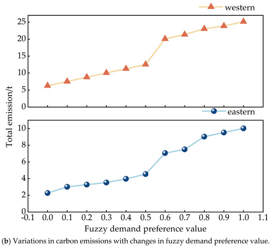
Figure 12. Sensitivity analysis of fuzzy demand preference values.

The results show that as the fuzzy demand preference value increases, both total transportation cost and carbon emissions also increase. This indicates that to improve customer satisfaction by meeting their demands, both total transportation cost and carbon emissions are increased. It is not possible to simultaneously achieve economic efficiency, environmental sustainability, and demand reliability. As a result, cargo carriers need to consider various factors and choose the best path based on their fuzzy demand preference value. The goal is to meet customer demand as much as possible while minimizing total transportation cost and carbon emissions.

5.3.5. Comparison of Single-Mode Transportation and Multimodal Transportation

Many cargo carriers prefer a single transportation mode, such as single-highway or single-railway transportation. Therefore, this paper compares multimodal transportation with single-mode transportation. Based on the analysis above, the fuzzy demand preference value $\beta$ is set to 0.8, and the carbon tax rates in the eastern and western regions are set at RMB 0.7 and 0.4/kg, respectively. Five transportation orders with different starting points, destinations, and demand volumes are addressed, using the multimodal transportation network examples in the eastern and western regions. These are shown in Table 12. The average of the optimal solutions for each order is used for the comparison analysis; the value for single-mode transportation is the average of single-highway and single-railway transportation. Figure 13 compares costs, time, and carbon emissions for different transportation modes.

Table 12. Transportation order form.

Order Number	Start-End	Demand
Order 1	1-8	[120, 140, 160, 180]
Order 2	1-13	[20, 40, 60, 80]
Order 3	2-10	[200, 220, 230, 260]
Order 4	3-12	[10, 30, 50, 70]
Order 5	5-10	[60, 80, 100, 120]

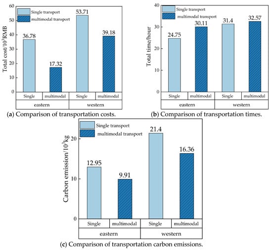
Figure 13. Comparison of modes of transportation.

Figure 13 shows that multimodal transportation is significantly more cost-effective than single-mode transportation. This reflects its advantages with respect to economic efficiency. Specifically, in the eastern region, the total transportation cost of multimodal transportation is 52.91% lower than that of single-mode transportation. In the western region, the decrease is 27.05%. This difference is mainly due to the more developed multimodal network in the eastern region; this provides more convenient conditions for multimodal transport. In regions with more advanced transportation networks, multimodal transportation offers greater economic advantages. Additionally, by incorporating railway and waterway transportation modes, multimodal transportation effectively reduces carbon emissions. However, since multimodal transport involves integration and transfer between different modes of transportation, single-mode transport has a slight advantage in terms of transportation efficiency. As such, cargo carriers should select the transportation mode based on timeliness requirements. For cargo deliveries that are less urgent, multimodal transport can be an effective choice for reducing logistics costs and achieving green transportation.

6. Conclusions

This study addresses the multimodal transportation route optimization problem under carbon tax policies, and then considers regional differences. A bi-objective optimization model is developed, which considers both total transportation cost and time. A fuzzy adaptive non-dominated sorting genetic algorithm is designed to solve the problem addressed by the model. The model-based problem-solving and case analysis approaches lead to the following conclusions:

(1)

An increase in the carbon tax rate plays a positive role in reducing carbon emissions during transportation. Its effectiveness varies across regions. Therefore, when formulating and implementing low-carbon policies, relevant authorities should tailor their approaches to local conditions and consider differences in regional transportation structures, multimodal infrastructure, and economic levels;

(2)

An increase in the fuzzy demand preference value can increase customer satisfaction by maximizing the fulfillment of demand. However, it also leads to higher transportation costs and carbon emissions for multimodal transport. Reliable demand, efficient transportation costs, and environmental sustainability cannot all be achieved simultaneously. Cargo carriers need to consider various factors when setting a reasonable fuzzy demand preference value;

(3)

Multimodal transportation offers a clear cost advantage over single-mode transportation, and can reduce carbon emissions during transportation. Cargo carriers should choose the transportation mode based on delivery urgency.

Multimodal transport is a highly complex system. This study has considered certain practical factors, such as uncertainty in freight demand and fixed departure schedules. Future research should further incorporate additional elements, including road congestion, capacity constraints, customer satisfaction, and multidimensional uncertainty conditions. This would further enhance the in-depth analysis of how these factors influence multimodal transport planning.

References

- IEA. CO2 Emissionsin 2022; IEA: Paris, France, 2023. [Google Scholar]
- Wang, M.X.; Yi, H.; Dongmei, G.; Jie, C. Optimal Emissions Implementation and Enterprises’ Abatement Investment Competition under the Carbon Tax Tool. Manag. Rev. 2021, 33, 17. [Google Scholar]
- Archetti, C.; Peirano, L.; Speranza, M.G. Optimization in multimodal freight transportation problems: A Survey. Eur. J. Oper. Res. 2022, 299, 1–20. [Google Scholar] [CrossRef]
- Elbert, R.; Müller, J.P.; Rentschler, J. Tactical network planning and design in multimodal transportation—A systematic literature review. Res. Transp. Bus. Manag. 2020, 35, 100462. [Google Scholar] [CrossRef]
- Zhang, H.; Liu, F.; Ma, L.; Zhang, Z. A hybrid heuristic based on a particle swarm algorithm to solve the capacitated location-routing problem with fuzzy demands. IEEE Access 2020, 8, 153671–153691. [Google Scholar] [CrossRef]
- Sun, Y.; Liang, X.; Li, X.; Zhang, C. A fuzzy programming method for modeling demand uncertainty in the capacitated road–rail multimodal routing problem with time windows. Symmetry 2019, 11, 91. [Google Scholar] [CrossRef]
- Peng, Y.; Gao, S.H.; Yu, D.; Xiao, Y.P.; Luo, Y.J. Multi-objective optimization for multimodal transportation routing problem with stochastic transportation time based on data-driven approaches. RAIRO-Oper. Res. 2023, 57, 1745–1765. [Google Scholar] [CrossRef]
- Zweers, B.G.; van der Mei, R.D. Minimum costs paths in intermodal transportation networks with stochastic travel times and overbookings. Eur. J. Oper. Res. 2022, 300, 178–188. [Google Scholar] [CrossRef]
- Peng, Y.; Luo, Y.J.; Jiang, P.; Yong, P.C. The route problem of multimodal transportation with timetable: Stochastic multi-objective optimization model and data-driven simheuristic approach. Eng. Comput. 2022, 39, 587–608. [Google Scholar] [CrossRef]
- Xie, L.; Cao, C.X. Multi-modal and multi-route transportation problem for hazardous materials under uncertainty. Eng. Optim. 2021, 53, 2180–2200. [Google Scholar] [CrossRef]
- Abbassi, A.; El hilali Alaoui, A.; Boukachour, J. Robust optimisation of the intermodal freight transport problem: Modeling and solving with an efficient hybrid approach. J. Comput. Sci. 2019, 30, 127–142. [Google Scholar] [CrossRef]
- Li, X.Y.; Sun, Y.; Qi, J.F.; Wang, D.Z. Chance-constrained optimization for a green multimodal routing problem with soft time window under twofold uncertainty. Axioms 2024, 13, 200. [Google Scholar] [CrossRef]
- Chang, T.-S. Best routes selection in international intermodal networks. Comput. Oper. Res. 2008, 35, 2877–2891. [Google Scholar] [CrossRef]
- Li, L.; Zhang, Q.W.; Zhang, T.; Zou, Y.B.; Zhao, X. Optimum route and transport mode selection of multimodal transport with time window under uncertain conditions. Mathematics 2023, 11, 3244. [Google Scholar] [CrossRef]
- Ziaei, Z.; Jabbarzadeh, A. A multi-objective robust optimization approach for green location-routing planning of multi-modal transportation systems under uncertainty. J. Clean. Prod. 2021, 291, 125293. [Google Scholar] [CrossRef]
- Huang, Y.Y.; Li, T.C.; Ma, L. A multi-objective multimodal transportation route planning model considering fuzzy node loads. Int. J. Innov. Comput. Inf. Control 2024, 20, 1331–1350. [Google Scholar]
- Zhang, M. Optimization of Multimodal Transport Routes Considering Carbon Emissions in Fuzzy Scenarios. Int. Core J. Eng. 2022, 8, 267–281. [Google Scholar]
- Zhang, Y.Z.; Ye, M.C.; Deng, L.Y.; Yang, J.L.; Hu, Y.Q. Path Optimization of Green Multimodal Transportation Considering Dynamic Random Transit Time. IAENG Int. J. Appl. Math. 2024, 54, 623–633. [Google Scholar]
- Sun, Y. A robust possibilistic programming approach for a road-rail intermodal routing problem with multiple time windows and truck operations optimization under carbon cap-and-trade policy and uncertainty. Systems 2022, 10, 156. [Google Scholar] [CrossRef]
- Liu, S.C. Multimodal transportation route optimization of cold chain container in time-varying network considering carbon emissions. Sustainability 2023, 15, 4435. [Google Scholar] [CrossRef]
- Zhang, H.Z.; Huang, Q.; Ma, L.; Zhang, Z.Y. Sparrow search algorithm with adaptive t distribution for multi-objective low-carbon multimodal transportation planning problem with fuzzy demand and fuzzy time. Expert Syst. Appl. 2024, 238, 122042. [Google Scholar] [CrossRef]
- Wu, C.Y.; Zhang, Y.; Xiao, Y.; Mo, W.I.; Xiao, Y.; Wang, J. Optimization of multimodal paths for oversize and heavyweight cargo under different carbon pricing policies. Sustainability 2024, 16, 6588. [Google Scholar] [CrossRef]
- Zhu, C.; Zhu, X. Multi-objective path-decision model of multimodal transport considering uncertain conditions and carbon emission policies. Symmetry 2022, 14, 221. [Google Scholar] [CrossRef]
- Zhang, T.; Cheng, J.; Zou, Y. Multimodal transportation routing optimization based on multi-objective Q-learning under time uncertainty. Complex Intell. Syst. 2024, 10, 3133–3152. [Google Scholar] [CrossRef]
- Xu, X.; Wang, H.; Deng, P. Exploring the Optimization of Synchromodal Transportation Path under Uncertainties. J. Mar. Sci. Eng. 2023, 11, 577. [Google Scholar] [CrossRef]
- Jiang, C. Research on Optimizing Multimodal Transport Path Under the Schedule Limitation Based on Genetic Algorithm; IOP Publishing: Bristol, UK, 2022. [Google Scholar]
- Dong, J.-Y.; Wan, S.-P. A new trapezoidal fuzzy linear programming method considering the acceptance degree of fuzzy constraints violated. Knowl.-Based Syst. 2018, 148, 100–114. [Google Scholar] [CrossRef]
- Iwamura, K.; Liu, B.D. A genetic algorithm for chance constrained programming. J. Inf. Optim. Sci. 1996, 17, 409–422. [Google Scholar] [CrossRef]
- Deb, K.; Pratap, A.; Agarwal, S.; Meyarivan, T. A fast and elitist multiobjective genetic algorithm: NSGA-II. IEEE Trans. Evol. Comput. 2002, 6, 182–197. [Google Scholar] [CrossRef]
- Ma, H.P.; Zhang, Y.J.; Sun, S.Y.; Liu, T.; Shan, Y. A comprehensive survey on NSGA-II for multi-objective optimization and applications. Artif. Intell. Rev. 2023, 56, 15217–15270. [Google Scholar] [CrossRef]
- Yang, L.J.; Zhang, C.; Wu, X. Multi-objective path optimization of highway-railway multimodal transport considering carbon emissions. Appl. Sci. 2023, 13, 4731. [Google Scholar] [CrossRef]
- Zhang, X.; Jin, F.-Y.; Yuan, X.-M.; Zhang, H.-Y. Low-carbon multimodal transportation path optimization under dual uncertainty of demand and time. Sustainability 2021, 13, 8180. [Google Scholar] [CrossRef]
- Chen, D.D. Roubst Optimisation of Container Multimodal Transportation Route Under Uncertainty; Southeast University: Nanjing, China, 2020. [Google Scholar]
- Li, X.D.; Kuang, H.B.; Zhao, Y.Z.; Liu, T.; Wu, H. An Empirical Study on Low-carbon and Multimodal Transport in the Northeast China. Manag. Rev 2021, 33, 282–291. [Google Scholar]
- Lu, S.L.; Bai, Y.F. International practices of carbon taxation and lts enlightenment to achievementof carbon peak in 2030. Int. Tax. China 2021, 12, 21–28. [Google Scholar]
Disclaimer/Publisher’s Note: The statements, opinions and data contained in all publications are solely those of the individual author(s) and contributor(s) and not of MDPI and/or the editor(s). MDPI and/or the editor(s) disclaim responsibility for any injury to people or property resulting from any ideas, methods, instructions or products referred to in the content. |
© 2025 by the authors. Licensee MDPI, Basel, Switzerland. This article is an open access article distributed under the terms and conditions of the Creative Commons Attribution (CC BY) license (https://creativecommons.org/licenses/by/4.0/).