Slope Stability Analysis Based on the Explicit Smoothed Particle Finite Element Method

Abstract

A landslide is a common natural disaster that causes environmental damage, casualties and economic losses, which seriously affects the sustainable development of society. In geomechanics, it is one of the largest deformation problems. Herein, the GPU-accelerated explicit smoothed particle finite element method (eSPFEM) for large deformation analysis in geomechanics was developed on the CUDA platform based on high-performance computing using a self-designed eSPFEM program code. The eSPFEM combines the strain smoothing nodal integration techniques found in the particle finite element method (PFEM) framework, which allows for the use of low-order triangular elements without volume locking and avoids frequent information transfer and mapping errors between Gaussian points and particles in PFEM. A numerical simulation of slope instability using the eSPFEM and based on a strength reduction technique was conducted using various examples, including a cohesive homogeneous slope, a non-cohesive homogeneous slope, a non-homogeneous slope and a slope with a thin soft band. The calculation results show that the eSPFEM can be applied to slope stability analysis under different working conditions, simulating the entire process of slope instability initiation, sliding and reaccumulation, and obtaining reliable FOS values. A numerical simulation was conducted to analyse a landslide that occurred in the Zhangjiazhuang tunnel on the Lanzhou–Xinjiang high-speed railway line on 18 January 2016. A natural unsaturated soil slope, a soil slope with a high moisture content and a soil slope with a high moisture content subjected to an earthquake were analysed. The findings of this study are in good agreement with the actual slope failure conditions. The primary triggers identified for the landslide were heavy rainfall and earthquakes. The verification results indicate that the eSPFEM can effectively simulate an actual landslide case, showcasing high accuracy and applicability in simulating the large deformation behaviour of landslides.

1. Introduction

1.1. Background of Landslides

A landslide is a common natural disaster that causes environmental damage, casualties and economic losses and has a serious negative impact on the sustainable development of society. Landslides can pose a severe threat to human survival and the orderly development of land resources and are one of the most pressing environmental problems worldwide.

Landslides can cause considerable soil loss, thus exerting long-term adverse effects on agricultural production, such as reduced soil productivity, soil water-holding capacity and water quality in streams and rivers [1]. It has been estimated that during severe storm events, which occur once every 20–50 years, steep pasture slopes may experience a loss of up to 10% of their soil area, leading to 36% of personal property being damaged and even casualties [2,3]. Studies indicate that the recovery of soil productivity in areas affected by landslide erosion takes many years and annual forage yields are unlikely to reach more than 80% of those in non-eroded areas within a few decades [3].

Landslides usually cause considerable damage to infrastructure, as this natural phenomenon may leave railway piers broken, railways bent and collapsed, passenger lines shut down for a long time, buildings severely damaged or collapsed, mountain roads cut off, high-voltage transmission towers destroyed and residential electricity disrupted [4]. Moreover, landslides have been known to cause damage to underground structures [5,6], with reported cases of landslide-induced damage extending to oil pipelines, road tunnels and railway tunnels [7,8].

In addition, geological disasters caused by human activities, such as engineering construction and the mining of rock and soil masses, occur frequently [9]. These activities not only alter the original landscape but also destroy native vegetation, disrupt the habitat of native animals and disturb the ecosystem. Furthermore, such human activities cause disturbance and damage to the exposed failure surface of rock and soil mass [10,11].

To ensure the sustainable development of both nature and society, it is imperative to leverage efficient numerical simulation technology for evaluating and predicting landslide disasters. By doing so, we can effectively prevent the adverse consequences of landslides and significantly minimize their negative impact.

1.2. Numerical Analysis Method for Large Deformation in Geomechanics

Numerous problems concerning geological hazards and geotechnical engineering are related to large deformation problems, such as landslides, debris flows, infrastructure installations, underground structure collapse, static penetration tests, anchoring and pulling out and soil liquefaction and seepage failure [12,13,14].

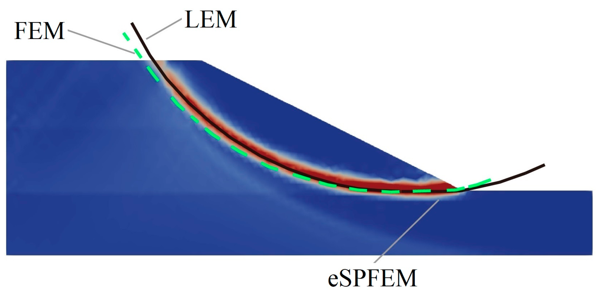
Although the traditional finite element method (FEM), which deals with small deformation, can describe the initial failure in the surface of the structure well, it may result in large mesh distortion when dealing with large deformations after the initial failure because the aforementioned method lacks stability and accuracy and is limited in terms of solving large deformation problems in geomechanics [13,15]. The large deformation of geomaterials under time-varying loads is a difficult problem in the field of geomechanics due to considerable soil structural deformation, complex contact conditions and nonlinear soil behaviour [16]. Therefore, the development of effective numerical simulation tools will be very helpful in analysing such problems. Large deformation finite element analysis has been widely used in geomechanics, and can numerically explain the problem of structural elements moving across relatively long distances in the soil [17]. Over the past 50 years, many numerical frameworks have been developed to describe and examine large deformation problems in geomechanics.

Thus, the arbitrary Lagrangian–Eulerian (ALE) method was developed, which combines the advantages of the Lagrange and Euler methods to alleviate the disadvantages of mesh deformation in the Lagrange method [18,19]. However, the computational efficiency of ALE depends on the division of the initial mesh, and the geometric calculation related to the mesh is cumbersome and complicated to implement [20,21].

Another method that was developed is the remeshing and interpolation technique with small strain (RITSS), which is an ALE-based approach [22,23]. After calculating each deformation step, RITSS conducts frequent mesh resection and variable interpolation according to the updated calculation boundary and repairs the deformed soil mass to avoid excessive distortion in the computed generated mesh [24]. However, this method requires specialised and user-dependent computer codes and scripts to control the processor, thus limiting its routine application in engineering practise [15].

The coupled Eulerian–Lagrangian (CEL) is another ALE-based method [25]. Unlike ALE, the mesh in the Lagrangian components of CEL is fixed and does not undergo mesh re-subdivision during calculation. As CEL is part of a commercial software, the method is more accessible. The analysis process is relatively straightforward, eliminating the need for users to program. Further, finite element models can be constructed entirely through graphical interfaces [26].

Moreover, the smooth particle hydrodynamics method (SPH) [27,28,29], which belongs to the group of mesh-free methods, avoids the deformation and distortion of the mesh by using a set of particles instead of the mesh in the traditional FEM method. The main advantage of SPH is that there is no need for a fixed computational mesh when calculating spatial derivatives, which can be replaced by analytical expressions based on smooth function derivatives [30]. However, the mesh-free method requires a proximity search and has a high computational cost. In addition, mesh-free methods usually require special processing techniques to deal with boundary conditions [31].

The material point method (MPM) is a mesh-based particle method [21,32,33,34,35] derived from the unit particle method in computational fluid dynamics [31]. Because MPM has Lagrangian and Eulerian characteristics, it avoids the problem of excessive mesh deformation when using the Lagrangian formula. By mapping between the material points and the mesh, mesh entanglement during the complete deformation process can be avoided [32].

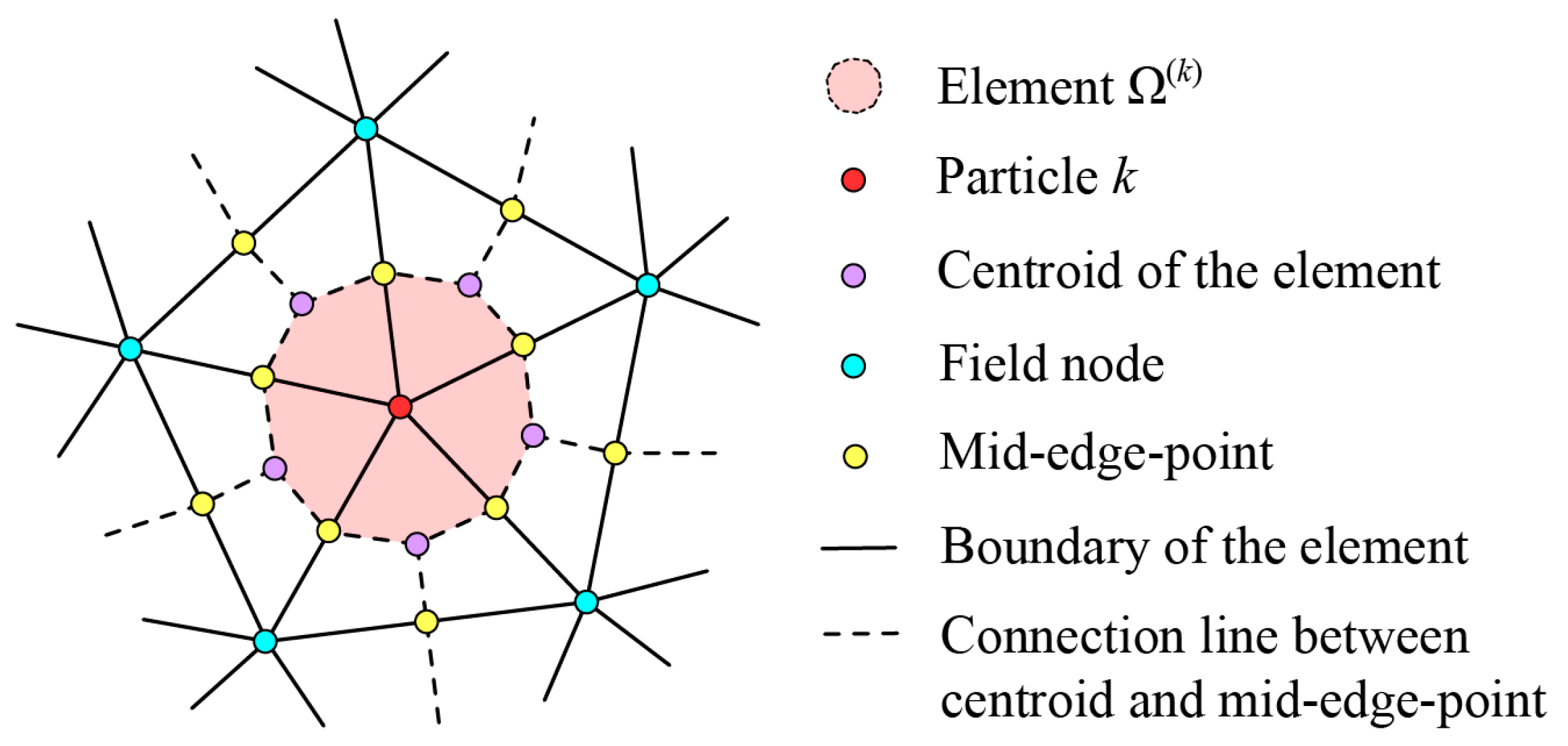
The particle finite element method (PFEM) is another mesh-based particle method [13,36], which uses particles to represent materials similar to the mesh-free particle approach. The Delaunay triangulation technique is used to connect these particles and build computational meshes. The boundary of the computing domain is determined using the α-shape method. The governing equations are solved using standard FEM. When the mesh deformation is deemed too large, the Delaunay triangulation technique is used to regenerate the mesh and avoid excessive mesh deformation. Therefore, the PFEM not only has the flexibility of the mesh-free particle method for arbitrary geometric shape alterations but also inherits the solid mathematical theoretical foundation of the traditional FEM [37], ensuring the accuracy and convergence of the calculations. However, the PFEM has two main problems: (1) volumetric locking due to the use of low-order elements and (2) mapping errors caused by frequent information transfer.

Recently, some new methods have been developed based on PFEM, such as the smoothed particle finite element method (SPFEM) with the introduction of strain smoothing technology [11,12,13,31], the edge-based smoothed particle finite element method (ES-PFEM) based on boundary integration [38], the node-based smoothed particle finite element method (NS-PFEM) based on nodal integration [39] and the stable node-based smoothed particle finite element method (SNS-PFEM) based on stable nodal integration [40,41]. However, it can be seen from Zhang et al. [13] that the calculation results of the SPFEM are conservative.

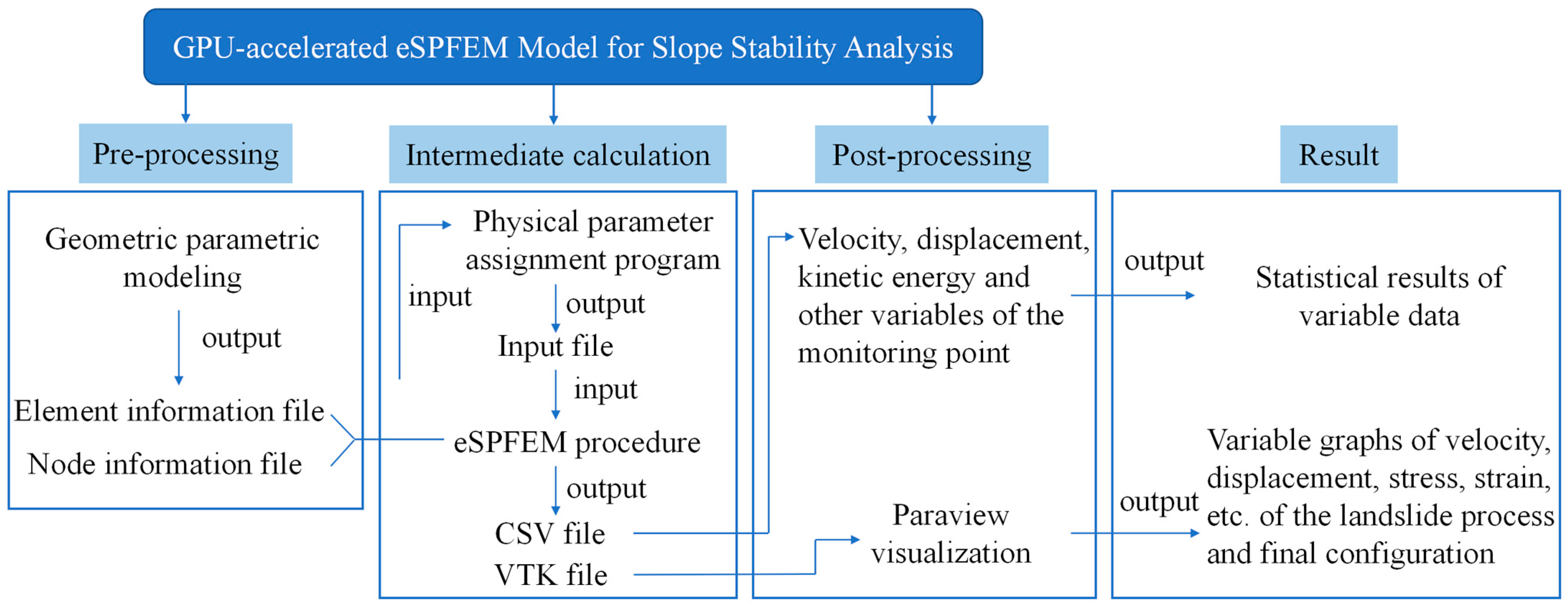
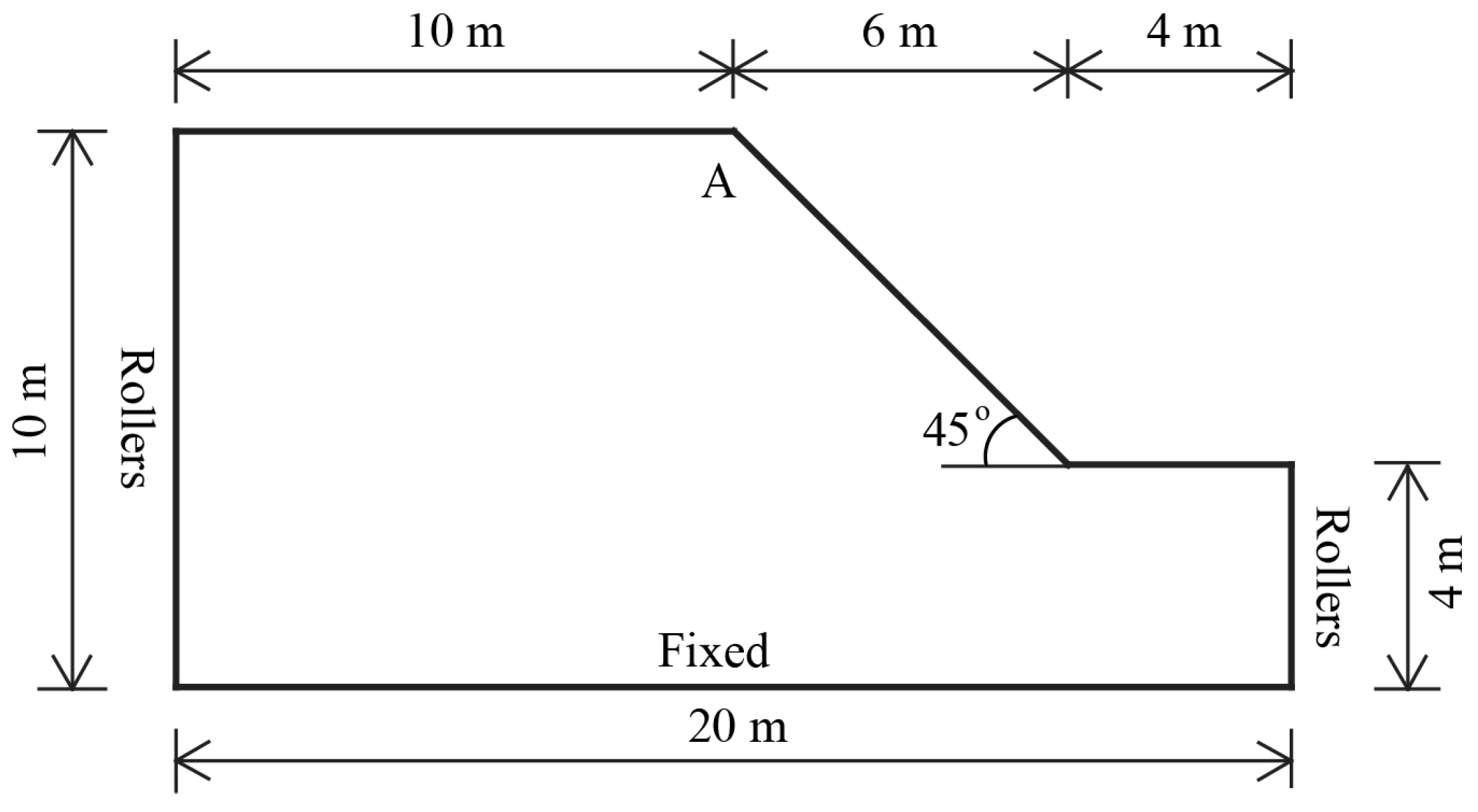
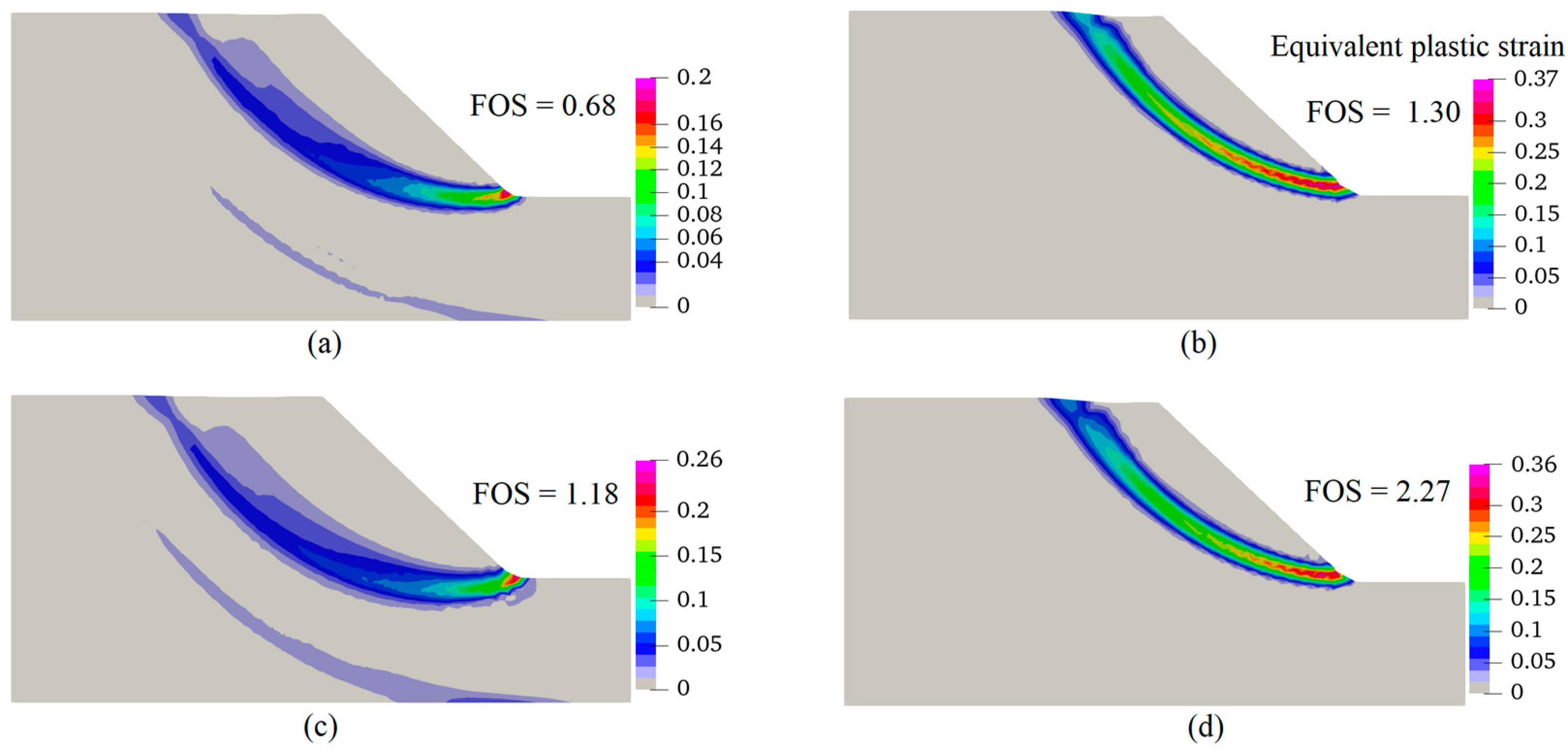
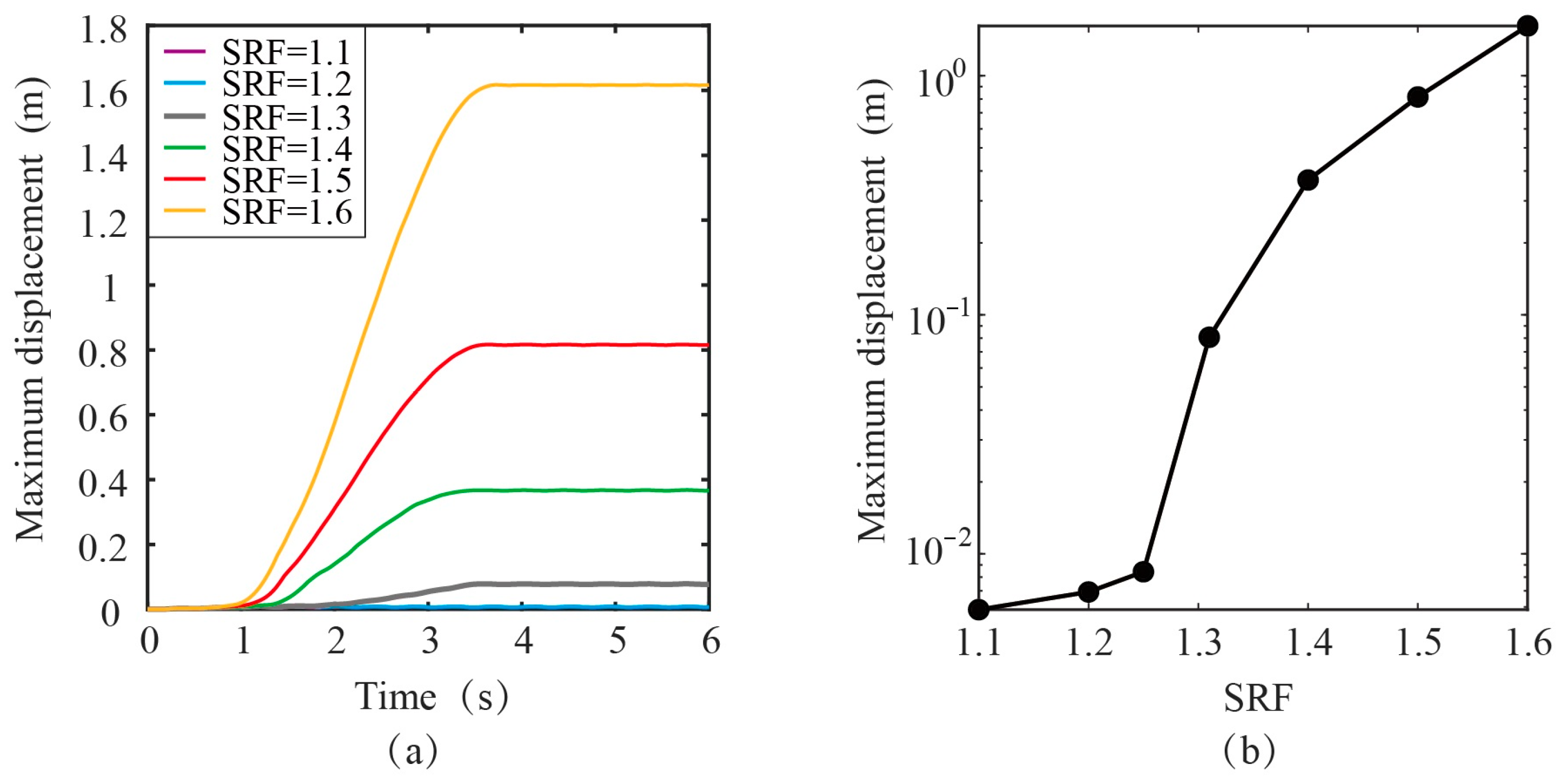
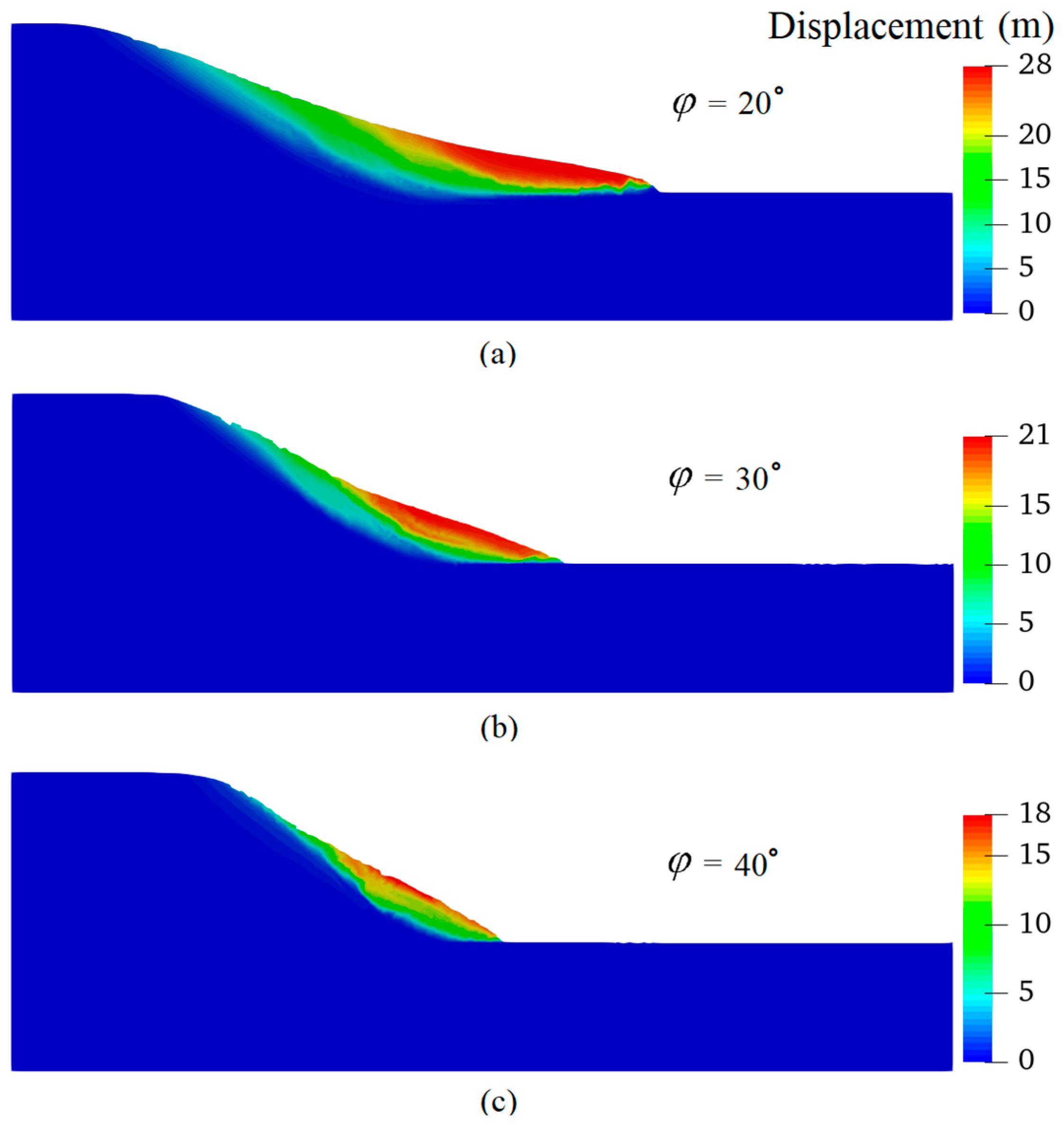
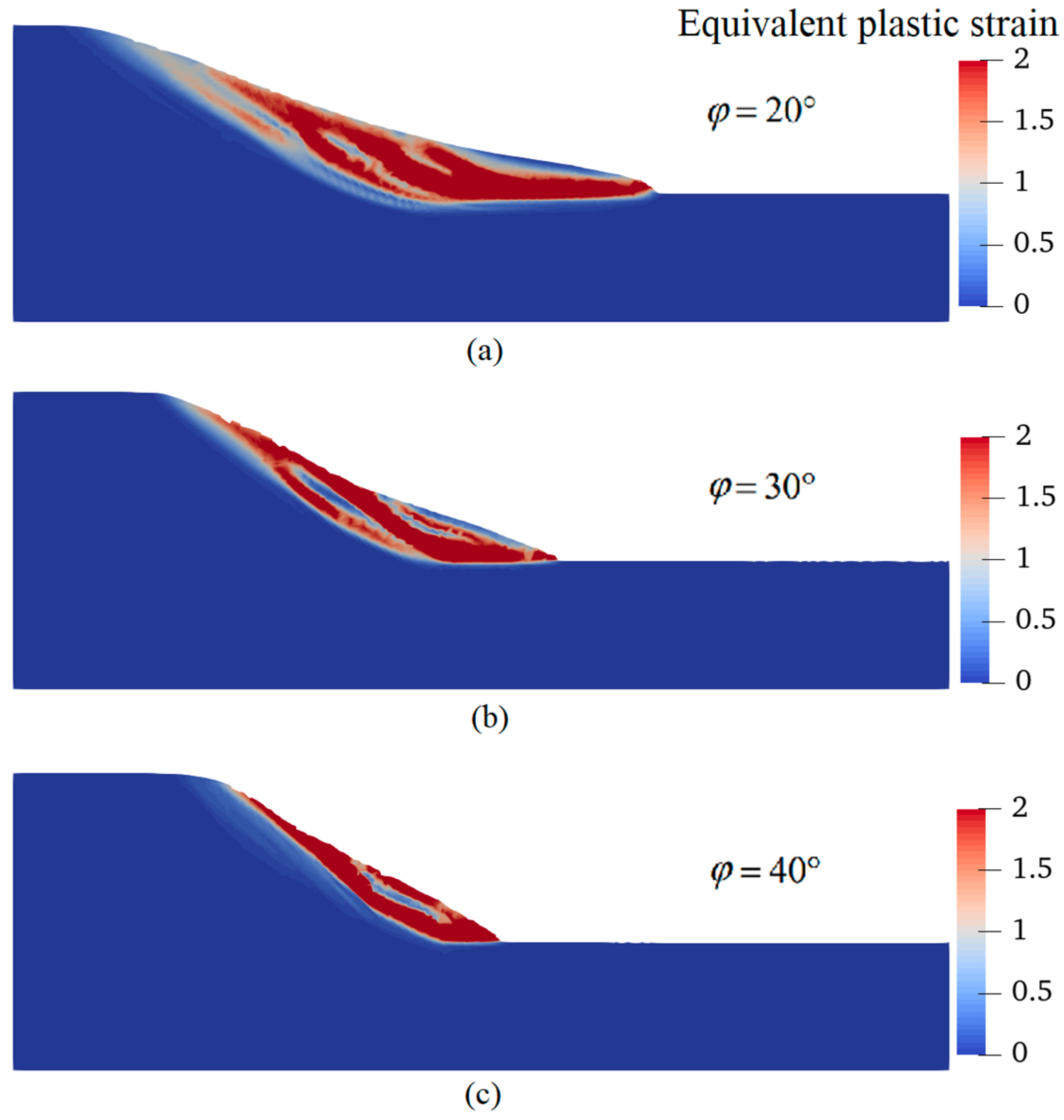
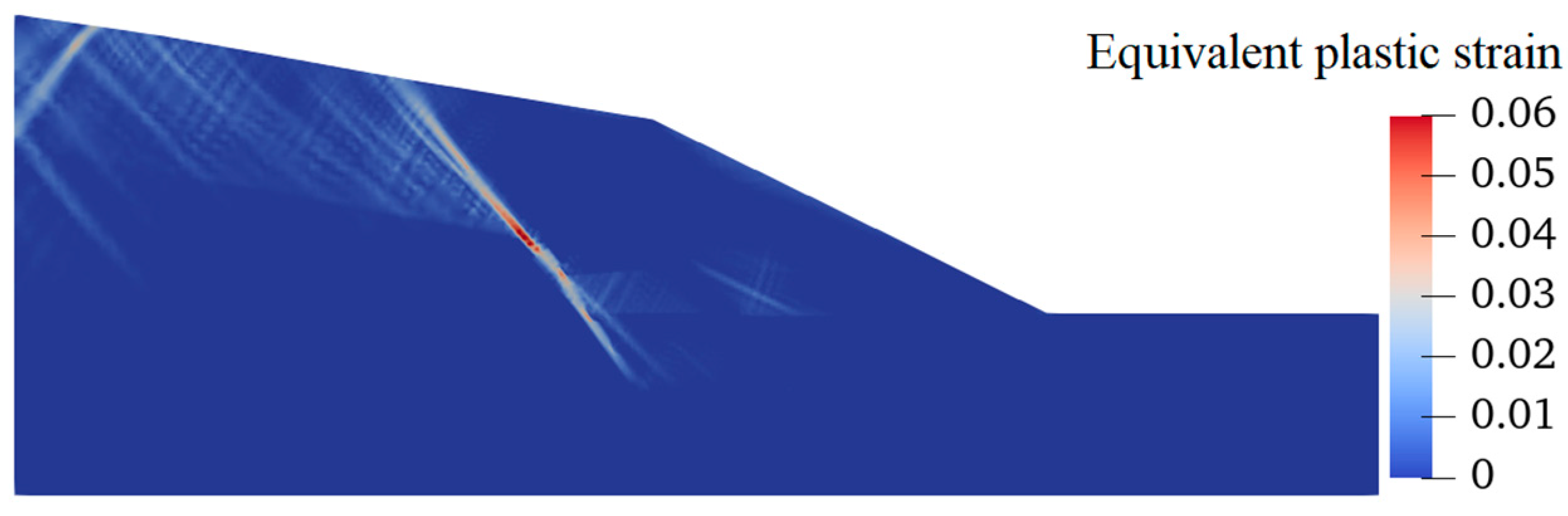
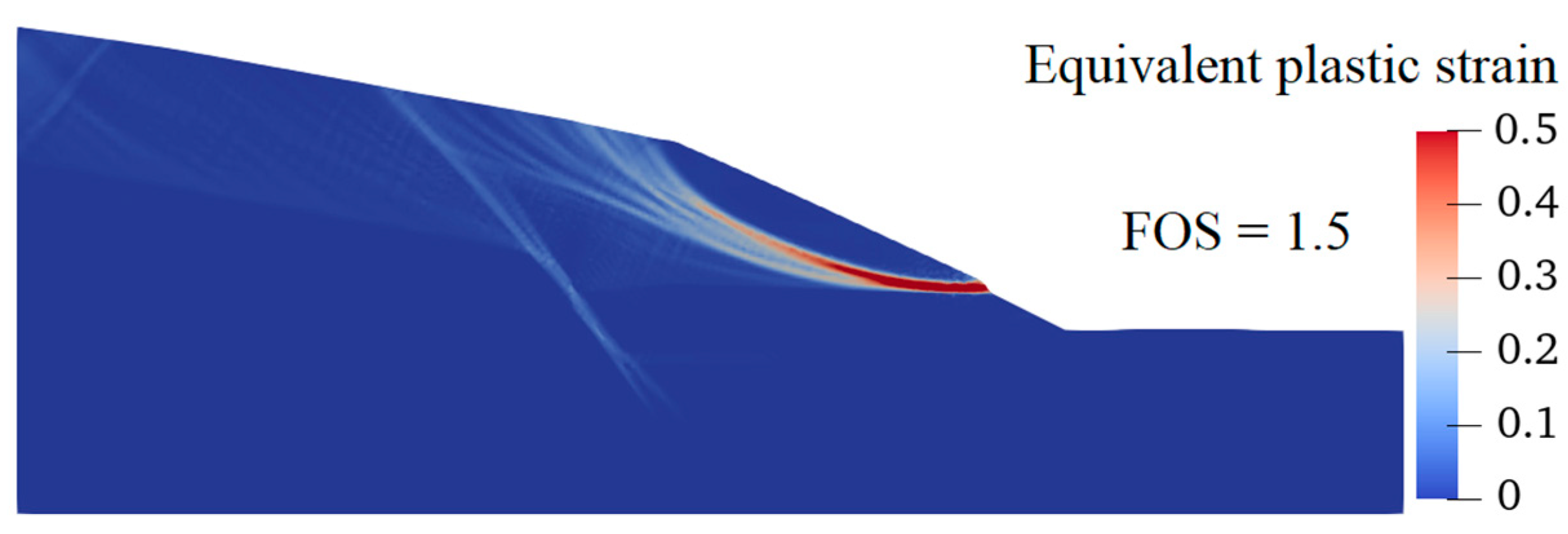
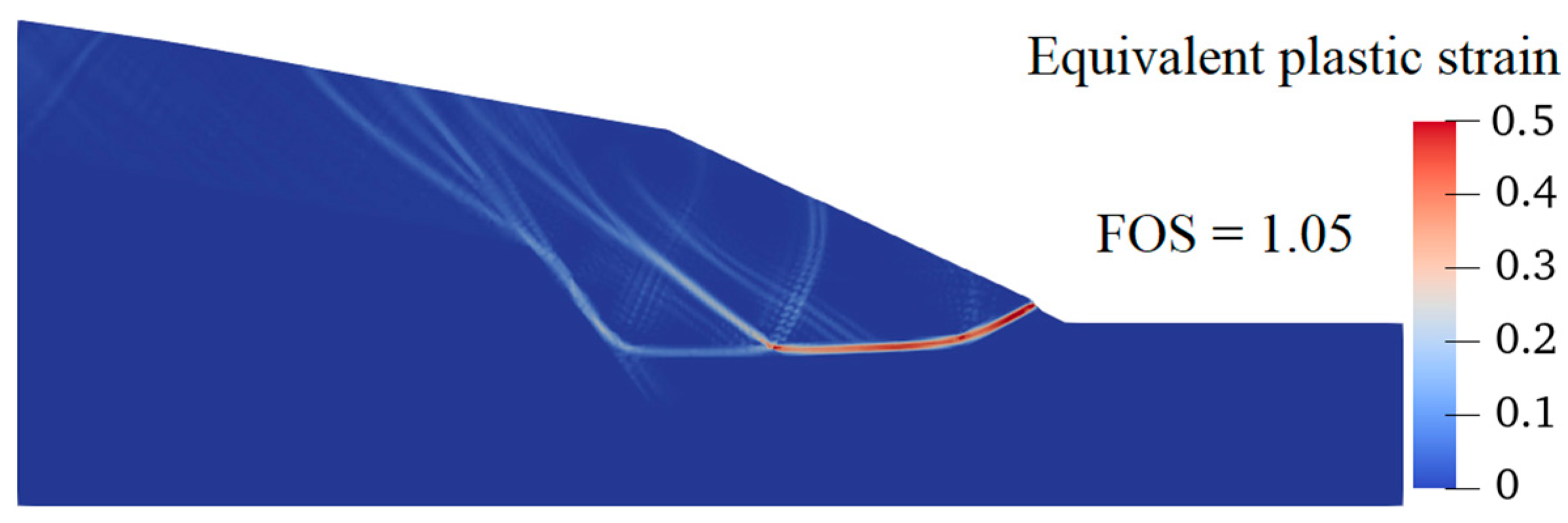
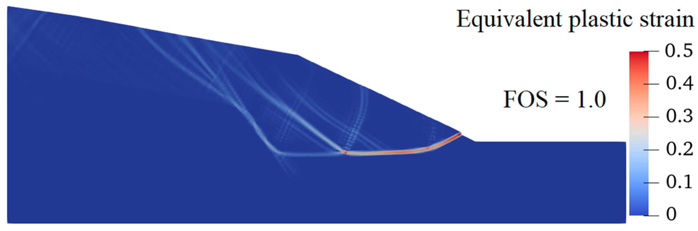
This study used the self-designed explicit SPFEM (eSPFEM) program code to develop a GPU-accelerated eSPFEM for large deformation analysis in geomechanics based on high-performance computing on the CUDA platform. The large deformation behaviour and final deposition state of the whole slope were simulated using the eSPFEM. The kinetic energy-based criterion combined with the strength reduction technique was used to calculate the factor of safety (FOS) value of the slope under different working conditions and the slope instability process.

2. The eSPFEM Approaches

2.1. Theoretical Background of SPFEM

In the PFEM calculation process, all field variables are carried by particles, and the numerical integration of all state variables is calculated at Gaussian points; thus, the frequent transfer of variable information between particles and Gaussian points is required. The information from field and state variables will inevitably produce errors during constant mapping, which will decrease the calculation’s accuracy and increase the complexity of the solution process. The SPFEM combines the strain smoothing nodal integration technique from the PFEM framework, divides the problem domain into strain smoothing elements associated with nodes (nodes are regarded as free particles) (Figure 1) and achieves continuous equilibrium in these strain smoothing elements [13]. Due to the use of nodal integrals in SPFEM, all field variables can be calculated directly on the particles, thus avoiding the errors from mapping variables between Gaussian points and particles in the original PFEM.

In SPFEM, a particle (node) carries a smooth element associated with it. In fact, mechanical equilibrium equations that are related to particles can be solved by these strain smoothing elements. As shown in Figure 1, the smooth elements associated with particle k are created by connecting the mid-edge points of the boundary of the triangular elements around particle k to the centroid of these elements. Each triangular element is divided into three quadrilateral subregions, each of which is connected to its nearest particle. The smooth element Ω^(k) associated with particle k is then created by combining each of the nearest subregions of all the triangular elements surrounding the particle k [13].

The steps in the calculation used to solve the standard SPFEM are as follows [11]:

(1)

Generate the particle cloud in the problem domain, and establish the initial finite element analysis model via Delaunay triangulation.

(2)

Re-identify the entire problem domain based on a α-shape approach.

(3)

Calculate the finite element incremental solution to the governing equations based on the strain smoothing nodal integration technique.

(4)

Integrate new model information, and update the position of the particles to form a new particle cloud while transferring the old particle information into the new particle model.

(5)

Return to step 1 and repeat until the stop condition associated with the problem is reached.

The SPFEM is known for its three main advantages: (1) all state variables can be directly calculated and stored on particles, avoiding frequent information transfer between Gaussian points and particles as well as the mapping error from mesh redivision in the original PFEM, thus ensuring computational efficiency. (2) In SPFEM, integration is performed via the strain smoothing nodal integration technique [42] so that low-order triangular elements can be used without volumetric locking; moreover, these elements are insensitive to mesh distortion and thus are conducive to large deformation analysis [31]. (3) The SPFEM has upper bound convergence [43], which provides a conservative estimate for geomechanical problems [13].

The eSPFEM, as proposed by Yuan et al. [11,31], adopts an explicit time integration scheme and strain smoothing nodal integration technique. The explicit time integration algorithm utilized in this study is based on Newton’s second law and employs the central difference method. The mass matrix in the explicit time integration algorithm is much simpler to derive than the stiffness matrix in the implicit time integration algorithm, and the mass matrix can be reduced to a diagonal matrix. Compared with the implicit SPFEM proposed by Zhang et al. [13], the eSPFEM has two features: (1) it has more concise formulas (no need to form stiffness matrices) and can solve large-scale problems with relatively high stability while taking less time. (2) The eSPFEM is easier to adapt from the existing FEM code; thus, the method can be applied more widely.

2.2. Theoretical Formulations of eSPFEM

2.2.1. Momentum Balance Equation

The mathematical formula for the conservation of linear momentum on a continuum is expressed as follows:

$$\rho \mathit{a}=\nabla \cdot \sigma +\rho \mathit{b}$$

(1)

where $\rho$ is the material density, a is the acceleration, σ is the Cauchy stress tensor and b is the specific body force density. By considering the principle of virtual displacement and the divergence theorem, the weak form of the equilibrium equation can be expressed as follows:

$${\displaystyle {\int }_{\mathrm{\Omega }}\delta \mathit{u}\cdot \rho \mathit{a}\mathrm{d}\mathrm{\Omega }}={\displaystyle {\int }_S\delta \mathit{u}\cdot {\mathit{\tau }}_S\mathrm{d}S}+{\displaystyle {\int }_{\mathrm{\Omega }}\delta \mathit{u}\cdot \rho \mathit{b}\mathrm{d}\mathrm{\Omega }}-{\displaystyle {\int }_{\mathrm{\Omega }}\delta \mathit{u}:\sigma \mathrm{d}\mathrm{\Omega }}$$

(2)

where u is the test function, generally assumed to satisfy $\delta \mathit{u}=0$, where the displacement boundary conditions are prescribed; Ω represents the configuration domain; and S represents the boundary and is the prescribed traction.

2.2.2. Spatial Discretisations

To solve Equation (2), the study domain must be spatially discretized. The configuration domain is first discretized into a group of particles under the eSPFEM framework and then the discretized domain becomes meshless via Delaunay triangulation using α-shape technique. The area of the smoothing element associated with particle k is calculated as follows:

$$A^{\left(k\right)}={\displaystyle {\int }_{{\mathrm{\Omega }}^{\left(k\right)}}\mathrm{d}\mathrm{\Omega }}=\frac{1}{3}{\displaystyle \sum _{j=1}^{N_e^{\left(k\right)}}{A}_e^j}$$

(3)

where Ω^(k) is the smoothing element associated with particle k, $N_e^{(k)}$ denotes the number of triangular elements related to particle k and $A_e^j$ is the shape function area of the jth triangular element around particle k. The smoothed-strain matrix ${\tilde{\mathit{B}}}^{(k)}$ can be expressed as follows:

$${\tilde{\mathit{B}}}^{(k)}=\frac{1}{A^{\left(k\right)}}{\displaystyle \sum _{j=1}^{N_e^{\left(k\right)}}\frac{1}{3}{A}_e^j{\mathit{B}}^j}$$

(4)

where ${\mathit{B}}^j$ represents the strain gradient matrix of the jth triangular element surrounding particle k. After discretization based on particle k, Equation (2) can be written as follows:

$${\displaystyle \sum _{k=1}^{Nn}\rho {\mathit{a}}_k{A}^{(k)}}={\displaystyle \sum _{k=1}^{Nn}{\displaystyle {\int }_S{\mathit{{\rm N}}}_k{\mathit{\tau }}_{S}dS}}+{\displaystyle \sum _{k=1}^{Nn}\rho {\mathit{b}}_k{A}^{(k)}}-{\displaystyle \sum _{k=1}^{Nn}{\tilde{\mathit{B}}}_{}^{(k)}{\mathit{\sigma }}_k{A}^{(k)}}$$

(5)

where Nn is the total number of particles in the computing domain. More details on the strain smoothing nodal integration technique can be found in Yuan et al. (2019) and Zhang et al. [12,13].

2.2.3. Time Discretization

For time integration, let the time step be Δt and the discrete time be $t^n=n·\mathrm{\Delta }t$, where n = 1, 2, 3, .... There are two main reasons for adopting explicit time integration, that is, (1) its easy implementation and (2) avoidance of massive computation loads when dealing with large-scale problems. Based on the central difference method, the acceleration is expressed as follows:

$${\mathit{a}}^n=\frac{1}{\mathrm{\Delta }t}\left({\mathit{v}}^{n+1/2}-{\mathit{v}}^{n-1/2}\right),{\mathit{a}}^n=\frac{{\mathit{f}}^n}{\mathit{M}}$$

(6)

The velocity and displacement can be expressed as follows:

$${\mathit{v}}^{n+1/2}={\mathit{v}}^{n-1/2}+\mathrm{\Delta }t\frac{{\mathit{f}}^n}{\mathit{M}}$$

(7)

$${\mathit{u}}^{n+1}={\mathit{u}}^n+\mathrm{\Delta }t{\mathit{v}}^{n+1/2}$$

(8)

where the mass matrix M is a diagonal matrix. Since calculating the stiffness of the entire element assemblage is no longer needed, it can be solved very efficiently at the element level.

2.2.4. Numerical Implementation

By incorporating the strain smoothing technique, the weak form of the linear momentum equation can be applied to the larger integration areas and the strain smoothing matrix, and Equation (2) can be expressed as follows:

$$\mathit{M}\mathit{a}={\mathit{F}}^{\mathrm{ext}}-{\mathit{F}}^{\mathrm{int}}$$

(9)

As per Equation (5), the external force ${\mathit{F}}^{\mathrm{ext}}$, internal force ${\mathit{F}}^{\mathrm{int}}$ and mass matrix M in Equation (9) are, respectively, expressed as follows:

$${\mathit{F}}^{ext}={\displaystyle \sum _{k=1}^{Nn}{\displaystyle {\int }_S{\mathit{{\rm N}}}_k{\mathit{\tau }}_{S}dS}}+{\displaystyle \sum _{k=1}^{Nn}\rho {\mathit{b}}_k{A}^{\left(k\right)}}$$

(10)

$${\mathit{F}}^{\mathrm{int}}={\displaystyle \sum _{k=1}^{N_n}{\tilde{\mathit{B}}}_{}^{\left(k\right)\mathrm{T}}{\mathit{\sigma }}_k{A}^{\left(k\right)}}$$

(11)

$$\mathit{M}={\displaystyle \sum _{k=1}^{Nn}\rho A^{\left(k\right)}}$$

(12)

The specific theory of the eSPFEM was reported by Yuan et al. [11,31].

2.3. GPU-Accelerated eSPFEM

In comparison to Central Processing Units (CPUs), Graphics Processing Units (GPUs) offer several advantages such as a higher number of cores, reduced thread scheduling costs and increased memory bandwidth. Furthermore, GPUs are capable of operating in Single-Instruction-Multiple-Data (SIMD) mode, which characterizes a class of parallel computers that execute the same operation on multiple data points simultaneously [12].

The entire calculation in the eSPFEM application is conducted using a CPU and GPU. The GPU performs the main computing work, and the intensive computing part of the application runs in parallel on thousands of CUDA cores. All data are stored in GPU memory and only transferred to CPU memory if Delaunay triangulation and occasional data output are required, which not only saves memory space but also improves computational efficiency. Based on the research results reported by Zhang et al. [12], the speed of GPU-accelerated numerical computation is considerably improved compared to CPU numerical computation, and the computational cost of GPU parallel computation is reduced by about 70%.

In the calculation process in the PFEM or SPFEM, there are many steps that require the same calculation for all cells or nodes (particles). Moreover, data dependencies are local and usually extend to only a few surrounding cells or nodes. As a result, most computations can be assigned to separate GPU threads for parallel execution. Compared with PFEM, the calculation process in the SPFEM has been considerably simplified owing to the use of the nodal integration scheme. The eSPFEM avoids the accumulation of the global stiffness matrix in implicit the SPFEM; thus, its calculation process is relatively simple, which can considerably promote GPU parallel computation [12]. If the eSPFEM calculation program in this study is applied to run the mesh model with about 5000 nodes, the calculation time can be between 5 and 30 min depending on the convergence conditions and the computing power can meet the requirements of analysis and calculation.

The GPU-accelerated eSPFEM calculation process for slope stability analysis is mainly divided into three parts, namely, pre-processing, intermediate calculation and post-processing. The specific technical route is shown in Figure 2.

3. Typical Examples of Slope Instability Calculated Using eSPFEM

To verify whether the eSPFEM can be used to analyse the problem of large deformation failure in slopes, numerical simulations of the eSPFEM based on the strength reduction technique were conducted for four typical slope examples, and the results were compared with the FOS values and critical failure surfaces reported in the references. The accuracy and applicability of the eSPFEM in analysing slope stability problems are discussed.

3.1. Cohesive Homogeneous Soil Slope

The strength reduction technique is usually insensitive to the dilatancy angle, Young’s modulus and research domain size; thus, the selection of these parameters is deemed unimportant in this analysis [44]. Therefore, for the Mohr–Coulomb yield criterion, the two parameters of soil cohesion and internal friction angle are mainly reduced, and the shear strength parameters are defined as follows:

$$\begin{array}{l}{c}_t=\frac{c}{\mathrm{SRF}}\\ {\phi }_t=\arctan \left(\frac{\tan \phi }{\mathrm{SRF}}\right)\end{array}$$

(13)

where $c_t$ and ${\phi }_t$ represent the reduced cohesion and internal friction angle, respectively, and SRF represents the shear strength reduction factor. The critical state of the slope can be identified by gradually increasing the SRF and reducing the soil strength.

Moreover, the two-dimensional, cohesive, homogeneous slope example reported by Cheng et al. [44] was recalculated and compared with the limit equilibrium method (LEM) results reported by Cheng et al. [44], the second-order cone programming-FEM (SOCP-FEM) results reported by Wang et al. [45] and the lower bound solution (LB), the upper bound solution (UB) and a mixed constant-stress smoothed-strain element using second-order cone programming (SOCP-αbES-FEM) results calculated by Zhou et al. [46].

The geometry and boundary conditions of the homogeneous slope are shown in Figure 3. The boundary conditions were set using rollers along the left and right vertical boundaries and were fully fixed at the base. The research domain was divided into 1417 elements and 2948 nodes using six-node triangular elements.

The material of the slope is modelled by assuming an elastic–perfectly plastic Mohr–Coulomb model with a Young’s modulus of E = 14 MPa, a Poisson’s ratio of ν = 0.3, a unit weight of γ = 20 kN/m³ and a dilatancy angle of 0°, and the values of cohesion c and the internal friction angle $\phi$ [44] are shown in

Table 1. Comparison of FOS values calculated using different numerical methods.

Method	Data Source	Case 1	Case 2	Case 3	Case 4
		$\mathit{c}=10 \mathbf{kPa}$ $\mathit{\phi }=5^{\mathbf{o}}$	$\mathit{c}=10 \mathbf{kPa}$ $\mathit{\phi }=25^{\mathbf{o}}$	$\mathit{c}=20 \mathbf{kPa}$ $\mathit{\phi }=5^{\mathbf{o}}$	$\mathit{c}=20 \mathbf{kPa}$ $\mathit{\phi }=35^{\mathbf{o}}$
LEM	Cheng et al., 2007 [44]	0.65	1.30	1.06	2.24
FEM	Cheng et al., 2007 [44]	0.69	1.36	1.20	2.28
LB	Zhou et al., 2022 [46]	0.68	1.31	1.18	2.26
UB	Zhou et al., 2022 [46]	0.70	1.36	1.20	2.34
SOCP-αbES-FEM	Zhou et al., 2022 [46]	0.69	1.33	1.19	2.30
SOCP-FEM	Wang et al. 2021 [45]	0.67	1.32	1.16	2.24
eSPFEM	this paper	0.68	1.30	1.18	2.27
Diff% *	—	1.49%	1.52%	1.72%	1.34%

* Diff% refers to the relative error of the FOS values between the results of this paper and SOCP-FEM [45].

.

The numerical simulation of slope failure using the eSPFEM is divided into two stages: (1) The positions of all the particles are fixed, and gravity is applied to these particles to achieve the initial stress field. (2) The particles are allowed to move, and after the initial shear failure, the unstable soil mass moves and reaches an equilibrium state at a new slope configuration. The strength reduction technique of gradually increasing the SRF value is adopted to obtain the FOS value of the slope. In reference to Yuan et al. [31], the landslide simulation time in this case is set to 6 s to obtain a new stable state for the slope after failure.

Table 1 shows the FOS values of the slope calculated using different methods and strength parameters. Although small differences are noted in the FOS results between the different methods in this example, these results are generally consistent.

The equivalent plastic strain distribution of the slope in the unstable state calculated using the eSPFEM is shown in Figure 4. Equivalent plastic strain refers to the plastic strain generated by equating six plastic strain components into a uniaxial tensile force, which is scalar. The equivalent plastic strain is expressed as follows:

$${\epsilon }_{\mathrm{eq}}^P=\sqrt{\frac{2}{3}{\mathbf{e}}^p:{\mathbf{e}}^p}$$

(14)

where ${\mathbf{e}}^p$ refers to the plastic strain tensor [12,20].

By comparing (a) and (b) (or (c) and (d)) in Figure 4, it can be observed that the potential failure volume of the slope decreases with an increasing friction angle $\phi$. By comparing (a) and (c) shown in Figure 4, it can be found that the potential failure volume increases with increasing cohesion c because the critical failure surface will be deeper when the cohesion strength is higher, which is consistent with the results obtained by Zhou et al. [46].

To demonstrate the ability of the eSPFEM to simulate the failure of a slope with large deformation, the slope instability state from SRF = 1.1 to SRF = 1.6 in Case 2 (c = 10 kPa; $\phi =25^{\mathrm{o}}$) was simulated. We monitored the horizontal displacement of point A located at the edge of the slope top (Figure 3).

Figure 5a,b show the relationship between the maximum horizontal displacements of point A and simulation time and the relationship between the maximum horizontal displacements of point A and different SRF values, respectively. When SRF is <1.30, displacement convergence can be obtained using only a few iterations. However, when SRF is ≥1.30 in the early calculation stage (when the simulation time is less than 2 s), calculating the small deformation stage cannot achieve convergence. However, in the later stage of large deformation, the relationship between the maximum displacement and the simulation time presents a convex curve. It can be inferred that, in the post-instability stage, unstable soil will become stable again.

Figure 6 shows the final slope configurations and equivalent plastic strain distribution for different SRF values calculated using the eSPFEM. As can be seen from Figure 6, when the SRF is 1.1, the slope is in a stable state, and the plastic zone begins to develop near the slope toe and extends further upwards into the middle part of the slope. When the SRF is 1.2, a thin band of plastic strain localisation appears, while the thin layer of plastic strain near the slope top is very dim, which indicates that the slope has not completely failed. When the SRF is ≥1.3, a continuous shear band of plastic strain localisation is detected, and the local failure is accompanied by a considerable displacement increment. The occurrence of slope failure was conclusively demonstrated. Once the shear band is completely formed, the soil above the shear band will slide downwards on the sliding surface, and the friction opposite to the sliding direction will eventually dissipate the energy of the system and stop the movement.

In addition, Figure 6d–f indicate that, in the large deformation stage, the process of soil mass continuing to produce displacement and tending towards stability after slope instability can also be simulated. Clearly, the eSPFEM can effectively address the problem of large deformation and the failure of cohesive homogeneous soil slopes, and can reasonably predict the final configuration of the slope.

3.2. Non-Cohesive Homogeneous Soil Slope

To further demonstrate the ability of the eSPFEM in analysing the stability of sandy soil slopes, the eSPFEM was used to calculate stability in an example from Huang et al. [47] using MPM for the failure of a non-cohesive homogeneous soil slope. The geometry and boundary conditions of the homogeneous slope are shown in Figure 7. The research domain was divided into 5510 elements and 11,299 nodes using six-node triangular elements.

The material of the slope is modelled by assuming an elastic–perfectly plastic Drucker–Prager model with a Young’s modulus of E = 70 MPa, Poisson’s ratio of ν = 0.3, cohesion of c = 0 kPa, unit weight of γ = 20 kN/m³, dilatancy angle of $\psi$ = 0° and internal friction angles of 20°, 30° and 40°, respectively [47]. According to Huang et al. [47], when the friction angle is 45°, the FOS of the slope is 1.0, and when the friction angle is less than 45°, the slope is deemed unstable.

Figure 8 shows the final configurations of the non-cohesive soil slopes for different internal friction angles calculated using eSPFEM. The collapse of the non-cohesive soil slope is caused by gravity, and the soil particles undergo a considerable deformation and material flow process after the failure; thereafter, the slope reaches a stable state under the new slope configuration. The final configurations of the slope calculated using the eSPFEM are almost consistent with those of the MPM [47]. The displacement at the landslide decreases with increasing internal friction angle because a larger internal friction angle results in greater dissipation of plastic energy; therefore, the less potential energy is converted into kinetic energy.

The reposed angles of slopes for different internal friction angles calculated using MPM [47] and the eSPFEM are shown in

Table 2. Reposed angles of the non-cohesive soil slope for various internal friction angles.

Method	Data Source	Internal Friction Angles
		$\mathit{\phi }={20}^{\mathbf{o}}$	$\mathit{\phi }={30}^{\mathbf{o}}$	$\mathit{\phi }={40}^{\mathbf{o}}$
MPM	Huang et al., 2015 [47]	15.2°	22°	29°
eSPFEM	This paper	15°	22°	29°
Diff% *	—	1.32%	0	0

* Diff% refers to the relative error of the reposed angles between the results of this paper and MPM [47].

, wherein it can be noted that the results of the two methods have little error. As shown in Table 2, the reposed angle increases with increasing internal friction angle, and the difference between the reposed angle and the internal friction angle increases with increasing internal friction angle. In addition, the reposed angle of the non-cohesive soil slope is always less than the internal friction angle [47].

Figure 9 shows the equivalent plastic strain distribution in the non-cohesive soil slope for different internal friction angles calculated using the eSPFEM. Unlike the cohesive soil slope, the non-cohesive soil slope has no obvious shear band. It can be observed that the eSPFEM can effectively solve the problem of large deformation and failure of non-cohesive homogeneous slopes.

3.3. Non-Homogeneous Soil Slope

An example of a non-homogeneous soil slope from Bishop [48] was calculated using the eSPFEM. The geometry and boundary conditions of the slope are shown in Figure 10. The research domain was divided into 1112 elements and 2337 nodes using six-node triangular elements. The non-homogeneous slope comprises three layers of soil with different materials. The soil material is modelled by assuming an elastic–perfectly plastic Mohr–Coulomb model with the parameters presented in

Table 3. Soil properties in the non-homogeneous slope [27].

Soil	E: MPa	ν	$\mathit{\phi }$: Degrees	c: kPa	$\mathit{\psi }$: Degress	γ: kN/m3
Soil 1	60	0.3	18	14.0	9	18.0
Soil 2	80	0.3	20	16.8	9	19.5
Soil 3	100	0.3	23	1.90	9	21.0

Note: E is Young’s modulus, ν is Poisson’s ratio, φ is internal friction angle, c is cohesion, γ is unit weight, ψ is dilatancy angle.

.

Table 4. FOS values of the non-homogeneous slope.

Method	LEM	FEM	SPH	XMPM	eSPFEM
Data source	Bishop, 1955 [48]	Bui et al., 2011 [27]	Bui et al., 2011 [27]	Liang et al., 2022 [49]	This paper
FOS	1.725	1.70	1.70	1.70	1.72

shows the FOS values of the non-homogeneous slope calculated using different methods. The calculation results from the LEM [48] are relatively large, while those from the FEM, SPH [27] and extended MPM (XMPM) [49] are smaller. The FOS values calculated using the eSPFEM are very close to those of the other four methods.

Figure 11 shows the plastic strain distribution in the eSPFEM and a comparison with the critical failure shear bands of the LEM and FEM. The critical slip surface provided by the eSPFEM and LEM is almost the same, while that from the FEM is a slightly larger slip circle. Therefore, the eSPFEM is also deemed suitable for the tackling the problem of non-homogeneous slope failure.

3.4. Slope with a Thin Soft Band

An example of a slope with a thin soft band, which was constructed by Cheng et al. [44], was calculated using the eSPFEM. The geometry and boundary conditions of the slope are shown in Figure 12. The research domain was divided into 2727 elements and 5622 nodes using six-node triangular elements. The soil behaviour was modelled using an elastic–perfectly plastic Mohr–Coulomb material, and the material properties are shown in

Table 5. Soil properties in slope with a thin soft band [44].

Soil	E: MPa	ν	$\mathit{\phi }$: Degress	c: kPa	$\mathit{\psi }$: Degress	γ: kN/m3
Soil 1	14	0.3	35	20	0	19
Soil 2	14	0.3	25	0	0	19
Soil 3	14	0.3	35	10	0	19

.

Table 6. FOS values of the slope with a thin soft band.

Method	LEM	FEM	eSPFEM
Data source	Cheng et al., 2007 [44]	Cheng et al., 2007 [44]	This paper
FOS	0.927	0.86	0.90

shows the FOS values of the slope calculated using different methods. The results calculated using the eSPFEM are within the range of the other two methods.

Figure 13 shows the equivalent plastic strain distribution in the eSPFEM and a comparison with the critical failure shear band of the LEM. The critical failure positions calculated using the two methods are very similar. The development of the critical failure surface is considerably influenced by the thin soft band, and the shear band is located in soil layer 2, with a low shear strength on the steeper lower slope.

The calculated results for the aforementioned four typical landslide examples indicate that the eSPFEM can be applied to slope stability analysis under different working conditions, simulating the entire process of slope instability initiation, sliding and reaccumulation and obtaining reliable FOS values. The computed shear bands, final configurations and FOS values consistently align well with results reported in existing literature. Consequently, the subsequent section employed the eSPFEM to investigate actual landslide cases, aiming to explore its applicability and accuracy in complex slope scenarios.

4. Typical Landslide Case Verification

4.1. Condition of the Study Area

The Loess Plateau in western China is typical of areas with a fragile geological environment; thus, the area suffers from frequent geological disasters due to vegetation destruction, soil erosion and poor engineering properties (such as high pore ratio, developed joints and strong water sensitivity) [50,51]. The simulation case selected was the landslide that occurred in the Zhangjiazhuang tunnel on the Lanzhou–Xinjiang high-speed railway line in a mudstone hilly area of the Loess Plateau in China on 18 January 2016.

The climate in the study area is a typical temperate semi-arid plateau continental climate. In the dry season, the rainfall is low and the duration is short, and the surface water formed via the rainfall quickly evaporates after transient infiltration into the loess [52]. During the rainy season (usually from July to September), substantial precipitation is transferred to underground storage. After the fracture, the groundwater in the fracture zone has high saturation, and the contribution of concentrated precipitation to the groundwater recharge is remarkable.

Seismic activity is also frequent in the study area. In fact, the Ledu Seismic Station (about 19 km away from the Zhangjiazhuang tunnel) conducted borehole strain observations in three directions and detected clear jump strain data at 0:43 on 18 January 2016. At nearly 0:44 on the same day, the vertical pendulum tiltmeter of the Menyuan Seismic Station (about 150 km away from the Zhangjiazhuang tunnel) also recorded a clear aberration [53]. The small earthquake, which did not have a significantly seismic sensation, was thought to have triggered this landslide.

Zhou et al. [53] conducted numerical simulations based on field investigation, borehole surveys, seismic activity and rainfall records analysis in the area to determine the geological characteristics and landslide mechanism of the site. They proposed that the causes of the landslide were as follows: (1) There was a natural sliding layer in the slope, which led to stress concentration and displacement failure in the slope. (2) Before the landslide occurred, the groundwater was directly replenished by the extreme rainfall, which then saturated the soil layer and developed the seepage channel. (3) Under no drainage conditions, the earthquake intensified the soil layer to quickly reach its limit state, resulting in a landslide.

4.2. Model Building

A ridge profile is selected for slope stability analysis, and an elastic–perfectly plastic Mohr–Coulomb model is used to describe the stress–strain behaviour in the slope. The material parameters in this study were the same as those of Zhou et al. [53], and the shear strength indexes were obtained from the consolidated quick direct shear test of Zhou et al. [53].

The geometry, soil material distribution and boundary conditions in the slope problem are shown in Figure 14. According to Chen et al. [44], the results of finite element numerical simulations are not sensitive to the size of the research domain. Therefore, to save on the calculation time and costs, the horizontal distance and elevation of the research domain are reduced by 10 times according to the actual slope size.

The soil material comprises loess, silt, a fissure zone and mudstone. Zones A, B, C and D are identified as weak fracture zones located in four types of soil materials. Under heavy rainfall conditions, the rainwater flows into the weak fracture zone through the crack holes, and the soil gradually reaches saturation.

The mesh and particle distribution in the study domain are shown in Figure 15. The geometry of the research domain was divided into 8465 elements and 17,252 nodes using six-node triangular elements. In the slope surface, the slope bottom and near the slip area, a finer mesh distribution was adopted.

4.3. Numerical Simulation and Analysis

4.3.1. Natural Unsaturated Soil Slope

The material properties of the rock and soil mass when the slope is in its natural unsaturated state are shown in

Table 7. Material properties of the natural unsaturated soil slope.

Material	E: MPa	ν	$\mathit{\phi }$: Degress	c: kPa	γ: kN/m3
Loess	14.3	0.3	25.8	22.3	18.9
Silt	32.5	0.3	23.2	20.2	17.8
Fracture zone	35.1	0.3	30.1	10.0	18.1
Mudstone	53.8	0.3	35.1	27.8	18.1

. First, the initial stress field of the slope under its own gravity load is obtained under the conditions that the strain is zero and the material properties are not changed. Figure 16 shows the equivalent plastic strain distribution in this state. It can be observed that a plastic strain zone extends from the slope surface to the fracture zone at a steep angle; this indicates that a small crack exists in the slope itself. The high shear area indicates stress concentration. However, no integral sliding surface was noted, but the slope may be unstable.

The shear strength of the materials in the loess area and weak fracture area (zones A, B, C and D) is reduced to the limit state of the slope; moreover, the FOS value of the natural unsaturated soil slope was calculated to be 1.5, indicating that the slope is stable when the moisture content is low. Figure 17 shows the equivalent plastic strain distribution of the natural unsaturated soil slope in the limit equilibrium state.

4.3.2. Soil Slope with High Moisture Content

The material properties of the rock and soil mass when the moisture content of the slope is high are shown in

Table 8. Material properties of the soil slope with high moisture content.

Material	E: MPa	ν	$\mathit{\phi }$: Degress	c: kPa	γ: kN/m3
Loess	14.3	0.3	25.8	22.3	18.9
Silt	32.5	0.3	23.2	20.2	17.8
Fracture zone	53.8	0.3	35.1	27.8	18.1
Mudstone	35.1	0.3	30.1	10.0	18.1
Zone C (Saturation)	35.1	0.3	10.6	9.6	18.1
Zone D (Saturation)	53.8	0.3	13.6	7.1	18.1

. The strength indices of weak fracture zones (Figure 14) were changed to the material parameters in the saturation state, in which the cohesion c and friction angle $\phi$ of zone C and D were reduced. The FOS value of the soil slope with high moisture content is calculated to be 1.05, which is significantly lower than that of the natural unsaturated soil slope. This indicates that the slope is close to the unstable state when the soil in zones C and D become saturated with water. Figure 18 shows the equivalent plastic strain distribution in the soil slope with moisture content in the limit equilibrium state, wherein the shear band of the slope coincides with the weak fracture zone.

4.3.3. Soil Slope with High Moisture Content Subjected to an Earthquake

Because a small earthquake with no seismic sensation was detected on the day of the landslide, an acceleration of 0.05 m/s² was applied to simulate the pseudo-static acceleration of the earthquakes in the soil slope model with high moisture content. The material parameters of the rock and soil mass when the slope has high moisture content and there is the occurrence of an earthquake are shown in Table 8.

The FOS value of the slope with high moisture content under the influence of the earthquake is calculated to be 1.0. The slope is in a critical failure state, indicating that a small earthquake may trigger the landslide. Figure 19 shows the equivalent plastic strain distribution in the slope in the limit equilibrium state, wherein it can be noted that the distribution of the shear band is similar to that of the soil slope with high moisture content.

After extreme rainfall, groundwater enters the soil through loess settlement caves, ground fissures and rock joints. The undrained condition increased the groundwater level and static pore pressure in zones C and D (Figure 14), and the soil in this area was saturated. Although the intensity of the earthquake that occurred on 18 January was small, the increase in pore pressure caused by the earthquake led to the reduction of effective stress, which then decreased the shear strength, resulting in local damage and slope displacement. Under undrained conditions, local displacement will stimulate higher excess pore pressure, forming a cycle of increasing local displacement and rising pore pressure [53]. Finally, the slope was destroyed by the superposition of rainfall and earthquake.

5. Conclusions

PFEM not only has the flexibility of the mesh-free particle method for arbitrary geometric shape alterations but also inherits the solid mathematical theoretical foundation of the traditional FEM, ensuring the accuracy and convergence of the calculations. SPFEM combines the strain smoothing technique in the PFEM framework, divides the problem domain into strain smoothing elements associated with nodes and achieves a continuous equilibrium in these strain smoothing elements. Therefore, it is possible to use low-order triangular elements without volume locking, making them more adaptable to large-deformation distorted meshes. In addition, due to the use of nodal integrals in SPFEM, all field variables can be calculated directly on particles, thus avoiding frequent information transfer and errors from mapping between Gaussian points and particles in PFEM. The eSPFEM adopts an explicit time integration scheme and strain smoothing nodal integration technique. Compared with the implicit SPFEM, the formulas in the eSPFEM are more concise, and the eSPFEM is easier to adapt from existing FEM code.

In this study, the self-designed eSPFEM program code was used to develop the GPU-accelerated eSPFEM for large deformation analysis in the context of geomechanics on the CUDA platform based on high-performance computing. The kinetic energy-based criterion combined with the strength reduction technique was used in calculating the FOS value of the slope under different working conditions and the slope instability process.

To verify the accuracy and applicability of the eSPFEM for slope stability analysis, a numerical simulation of slope instability based on the strength reduction technique was conducted to calculate samples of a cohesive homogeneous slope, a non-cohesive homogeneous slope, a non-homogeneous slope and a slope with a thin soft band. By comparing the results of the FOS value and critical failure surface of the four typical landslide examples with those in the literature, it was found that the eSPFEM can be utilised for slope stability analysis under different working conditions because it can simulate the whole slope instability process and predict the large deformation behaviour and final deposition state of slope failure.

The landslide that occurred in the Zhangjiazhuang tunnel on the Lanzhou–Xinjiang high-speed railway line on 18 January 2016 was numerically simulated using the eSPFEM based on a strength reduction technique. The natural unsaturated soil slope, soil slope with high moisture content and soil slope with high moisture content subjected to an earthquake were analysed. By comparing the FOS values under different working conditions, it can be concluded that heavy rainfall and earthquakes are the main factors that have triggered this landslide. The findings of this study are in good agreement with the actual slope failure condition, and the verification results confirm the validity of the theoretical model. The eSPFEM can effectively and accurately simulate and verify the actual landslide, making it highly valuable for analysing the large deformation problems in geomechanics. The future work should focus on expanding the model to encompass three-dimensional profiles to enhance the applicability and reliability of the findings in practical scenarios.

References

1. Diwakar, K.C.; Dangi, H.; Naqvi, M.W.; Kadel, S.; Hu, L.B. Recurring Landslides and Debris Flows near Kalli Village in the Lesser Himalayas of Western Nepal. Geotech. Geol. Eng. 2023, 41, 3151–3168. [Google Scholar] [CrossRef]
2. Marden, M.; Arnold, G.; Gomez, B.; Rowan, D. Pre-and post-reforestation gully development in Mangatu Forest, East Coast, North Island, New Zealand. River Res. Appl. 2005, 21, 757–771. [Google Scholar] [CrossRef]
3. Rosser, B.J.; Ross, C.W. Recovery of pasture production and soil properties on soil slip scars in erodible siltstone hill country, Wairarapa, New Zealand. N. Z. J. Agr. Res. 2011, 54, 23–44. [Google Scholar] [CrossRef]
4. Wang, F.; Chen, Y.; Yan, K. A destructive mudstone landslide hit a high-speed railway on 15 September 2022 in Xining city, Qinghai province, China. Landslides 2023, 20, 871–874. [Google Scholar] [CrossRef]
5. Hungr, O.; Leroueil, S.; Picarelli, L. The Varnes classification of landslide types, an update. Landslides 2014, 11, 167–194. [Google Scholar] [CrossRef]
6. Wang, X.; Wang, H.; Liang, R.Y. A method for slope stability analysis considering subsurface stratigraphic uncertainty. Landslides 2018, 15, 925–936. [Google Scholar] [CrossRef]
7. Tian, X.; Song, Z.; Zhang, Y. Monitoring and reinforcement of landslide induced by tunnel excavation: A case study from Xiamaixi tunnel. Tunn. Undergr. Space Technol. 2021, 110, 103796. [Google Scholar] [CrossRef]
8. Dutta, S.; Hawlader, B. Pipeline–soil–water interaction modelling for submarine landslide impact on suspended offshore pipelines. Géotechnique 2019, 69, 29–41. [Google Scholar] [CrossRef]
9. Shahi, Y.B.; Kadel, S.; Dangi, H.; Adhikari, G.; Kc, D.; Paudyal, K.R. Geological Exploration, Landslide Characterization and Susceptibility Mapping at the Boundary between Two Crystalline Bodies in Jajarkot, Nepal. Geotechnics 2022, 2, 1059–1083. [Google Scholar] [CrossRef]
10. dos Santos, J.V.; Rangel, W.D.; Guimaraes, A.A.; Jaramillo, P.M.D.; Rufini, M.; Marra, L.M.; López, M.V.; da Silva, M.A.P.; Soares, C.R.F.S.; Moreira, F.M.D. Soil biological attributes in arsenic-contaminated gold mining sites after revegetation. Ecotoxicology 2013, 22, 1526–1537. [Google Scholar] [CrossRef]
11. Valentim dos Santos, J.; Varón-López, M.; Fonsêca Sousa Soares, C.R.; Lopes Leal, P.; Siqueira, J.O.; de Souza Moreira, F.M. Biological attributes of rehabilitated soils contaminated with heavy metals. Environ. Sci. Pollut. Res. 2016, 23, 6735–6748. [Google Scholar] [CrossRef] [PubMed]
12. Huang, Y.; Dai, Z.L. Large deformation and failure simulations for geo-disasters using smoothed particle hydrodynamics method. Eng. Geol. 2014, 168, 86–97. [Google Scholar] [CrossRef]
13. Yuan, W.H.; Wang, B.; Zhang, W.; Jiang, Q.; Feng, X.T. Development of an explicit smoothed particle finite element method for geotechnical applications. Comput. Geotech. 2019, 106, 42–51. [Google Scholar] [CrossRef]
14. Zhang, W.; Zhong, Z.H.; Peng, C.; Yuan, W.H.; Wu, W. GPU-accelerated smoothed particle finite element method for large deformation analysis in geomechanics. Comput. Geotech. 2021, 129, 103856. [Google Scholar] [CrossRef]
15. Zhang, W.; Yuan, W.H.; Dai, B.B. Smoothed particle finite-element method for large-deformation problems in geomechanics. Int. J. Geomech. 2018, 18, 04018010. [Google Scholar] [CrossRef]
16. Jia, X.; Zhang, W.; Wang, X.; Jin, Y.; Cong, P. Numerical Analysis of an Explicit Smoothed Particle Finite Element Method on Shallow Vegetated Slope Stability with Different Root Architectures. Sustainability 2022, 14, 11272. [Google Scholar] [CrossRef]
17. Tian, Y.; Cassidy, M.J.; Randolph, M.F.; Wang, D.; Gaudin, C. A simple implementation of RITSS and its application in large deformation analysis. Comput. Geotech. 2014, 56, 160–167. [Google Scholar] [CrossRef]
18. Vavourakis, V.; Loukidis, D.; Charmpis, D.C.; Papanastasiou, P. A robust finite element approach for large deformation elastoplastic plane-strain problems. Finite Elem. Anal. Des. 2013, 77, 1–15. [Google Scholar] [CrossRef]
19. Kardani, M.; Nazem, M.; Carter, J.P.; Abbo, A.J. Efficiency of high-order elements in large-deformation problems of geomechanics. Int. J. Geomech. 2015, 15, 04014101. [Google Scholar] [CrossRef]
20. Jin, Z.; Yin, Z.Y.; Kotronis, P.; Li, Z. Advanced numerical modelling of caisson foundations in sand to investigate the failure envelope in the HMV space. Ocean Eng. 2019, 190, 106394. [Google Scholar] [CrossRef]
21. Soga, K.; Alonso, E.; Yerro, A.; Kumar, K.; Bandara, S.; Kwan, J.S.H.; Koo, R.C.H.; Law, R.P.H.; Yiu, J.; Sze, E.H.Y.; et al. Trends in large-deformation analysis of landslide mass movements with particular emphasis on the material point method. Géotechnique 2016, 66, 248–273. [Google Scholar] [CrossRef]
22. Hu, Y.; Randolph, M.F. A practical numerical approach for large deformation problems in soil. Int. J. Numer. Anal. Methods Geomech. 1998, 22, 327–350. [Google Scholar] [CrossRef]
23. Yu, X.; Zou, D.; Kong, X.; Yu, L. Large-deformation finite element analysis of the interaction between concrete cut-off walls and high-plasticity clay in an earth core dam. Eng. Comput. 2017, 34, 1126–1148. [Google Scholar] [CrossRef]
24. Wang, D.; Randolph, M.F.; White, D.J. A dynamic large deformation finite element method based on mesh regeneration. Comput. Geotech. 2013, 54, 192–201. [Google Scholar] [CrossRef]
25. Qiu, G.; Henke, S.; Grabe, J. Application of a Coupled Eulerian–Lagrangian approach on geomechanical problems involving large deformations. Comput. Geotech. 2011, 38, 30–39. [Google Scholar] [CrossRef]
26. Wang, D.; Bienen, B.; Nazem, M.; Tian, Y.; Zheng, J.; Pucker, T.; Randolph, M.F. Large deformation finite element analyses in geotechnical engineering. Comput. Geotech. 2015, 65, 104–114. [Google Scholar] [CrossRef]
27. Bui, H.H.; Fukagawa, R.; Sako, K.; Wells, J.C. Slope stability analysis and discontinuous slope failure simulation by elasto-plastic smoothed particle hydrodynamics (SPH). Géotechnique 2011, 61, 565–574. [Google Scholar] [CrossRef]
28. Pastor, M.; Blanc, T.; Haddad, B.; Petrone, S.; Morles, M.S.; Drempetic, V.; Issler, D.; Crosta, G.B.; Cascini, L.; Sorbino, G.; et al. Application of a SPH depth-integrated model to landslide run-out analysis. Landslides 2014, 11, 793–812. [Google Scholar] [CrossRef]
29. Baêta-Neves, A.P.; Ferreira, A. Shaped charge simulation using SPH in cylindrical coordinates. Eng. Comput. 2015, 32, 370–386. [Google Scholar] [CrossRef]
30. Li, S.; Liu, W.K. Meshfree and particle methods and their applications. Appl. Mech. Rev. 2002, 55, 1–34. [Google Scholar] [CrossRef]
31. Yuan, W.H.; Liu, K.; Zhang, W.; Dai, B.; Wang, Y. Dynamic modeling of large deformation slope failure using smoothed particle finite element method. Landslides 2020, 17, 1591–1603. [Google Scholar] [CrossRef]
32. Sulsky, D.; Chen, Z.; Schreyer, H.L. A particle method for history-dependent materials. Comput. Methods Appl. Mech. Eng. 1994, 118, 179–196. [Google Scholar] [CrossRef]
33. Beuth, L.; Więckowski, Z.; Vermeer, P.A. Solution of quasi-static large-strain problems by the material point method. Int. J. Numer. Anal. Methods Geomech. 2011, 35, 1451–1465. [Google Scholar] [CrossRef]
34. Abe, K.; Soga, K.; Bandara, S. Material point method for coupled hydromechanical problems. J. Geotech. Geoenviron. 2014, 140, 04013033. [Google Scholar] [CrossRef]
35. Bandara, S.; Soga, K. Coupling of soil deformation and pore fluid flow using material point method. Comput. Geotech. 2015, 63, 199–214. [Google Scholar] [CrossRef]
36. Oñate, E.; Idelsohn, S.R.; Del Pin, F.; Aubry, R. The particle finite element method—An overview. Int. J. Comp. Methods Sing. 2004, 1, 267–307. [Google Scholar] [CrossRef]
37. Zhang, X.; Krabbenhoft, K.; Sheng, D.C.; Li, W.C. Numerical simulation of a flow-like landslide using the particle finite element method. Comput. Mech. 2015, 55, 167–177. [Google Scholar] [CrossRef]
38. Jin, Y.F.; Yuan, W.H.; Yin, Z.Y.; Cheng, Y.M. An edge-based strain smoothing particle finite element method for large deformation problems in geotechnical engineering. Int. J. Numer. Anal. Methods Geomech. 2020, 44, 923–941. [Google Scholar] [CrossRef]
39. Wang, Z.Y.; Jin, Y.F.; Yin, Z.Y.; Wang, Y.Z. A novel coupled NS-PFEM with stable nodal integration and polynomial pressure projection for geotechnical problems. Int. J. Numer. Anal. Methods Geomech. 2022, 46, 2535–2560. [Google Scholar] [CrossRef]
40. Jin, Y.F.; Yin, Z.Y.; Zhou, X.W.; Liu, F.T. A stable node-based smoothed PFEM for solving geotechnical large deformation 2D problems. Comput. Methods Appl. Mech. Eng. 2021, 387, 114179. [Google Scholar] [CrossRef]
41. Jin, Y.F.; Yin, Z.Y. Two-phase PFEM with stable nodal integration for large deformation hydromechanical coupled geotechnical problems. Comput. Methods Appl. Mech. Eng. 2022, 392, 114660. [Google Scholar] [CrossRef]
42. Franci, A.; Cremonesi, M.; Perego, U.; Oñate, E. A Lagrangian nodal integration method for free-surface fluid flows. Comput. Methods Appl. Mech. Eng. 2020, 361, 112816. [Google Scholar] [CrossRef]
43. Franci, A. Lagrangian finite element method with nodal integration for fluid–solid interaction. Comput. Part. Mech. 2021, 8, 389–405. [Google Scholar] [CrossRef]
44. Cheng, Y.M.; Lansivaara, T.; Wei, W.B. Two-dimensional slope stability analysis by limit equilibrium and strength reduction methods. Comput. Geotech. 2007, 34, 137–150. [Google Scholar] [CrossRef]
45. Wang, L.; Zhang, X.; Zaniboni, F.; Oñate, E.; Tinti, S. Mathematical optimization problems for particle finite element analysis applied to 2D landslide modeling. Math. Geosci. 2021, 53, 81–103. [Google Scholar] [CrossRef]
46. Zhou, X.W.; Liu, F.T.; Yin, Z.Y.; Jin, Y.F.; Zhang, C.B. A mixed constant-stress smoothed-strain element with a cubic bubble function for elastoplastic analysis using second-order cone programming. Comput. Geotech. 2022, 145, 104701. [Google Scholar] [CrossRef]
47. Huang, P.; Li, S.L.; Guo, H.; Hao, Z.M. Large deformation failure analysis of the soil slope based on the material point method. Computat. Geosci. 2015, 19, 951–963. [Google Scholar] [CrossRef]
48. Bishop, A.W. The use of the slip circle in the stability analysis of slopes. Géotechnique 1955, 5, 7–17. [Google Scholar] [CrossRef]
49. Liang, Y.; Chandra, B.; Soga, K. Shear band evolution and post-failure simulation by the extended material point method (XMPM) with localization detection and frictional self-contact. Comput. Method Appl. Mech. 2022, 390, 114530. [Google Scholar] [CrossRef]
50. Sun, W.Y.; Shao, Q.Q.; Liu, J.Y.; Zhai, J. Assessing the effects of land use and topography on soil erosion on the Loess Plateau in China. Catena 2014, 121, 151–163. [Google Scholar] [CrossRef]
51. Liang, C.Y.; Cao, C.S.; Wu, S.R. Hydraulic-mechanical properties of loess and its behavior when subjected to infiltration-induced wetting. Bull. Eng. Geol. Environ. 2018, 77, 385–397. [Google Scholar] [CrossRef]
52. Zhang, X.C.; Liu, W.Z.; Li, Z.; Zheng, F.L. Simulating site-specific impacts of climate change on soil erosion and surface hydrology in southern Loess Plateau of China. Catena 2009, 79, 237–242. [Google Scholar] [CrossRef]
53. Zhou, S.H.; Tian, Z.Y.; Di, H.G.; Guo, P.J.; Fu, L.L. Investigation of a loess-mudstone landslide and the induced structural damage in a high-speed railway tunnel. Bull. Eng. Geol. Environ. 2020, 79, 2201–2212. [Google Scholar] [CrossRef]
Figure 1. Construction of the smoothing element associated with particle [16].
Sustainability 16 00702 g001
Figure 2. Technical route.
Sustainability 16 00702 g002
Figure 3. Geometry and boundary conditions of the cohesive homogeneous slope problem.
Sustainability 16 00702 g003
Figure 4. Equivalent plastic strain distribution for SRF equal to FOS calculated using eSPFEM: (a) c = 10 kPa, φ = 5 o ; (b) c = 10 kPa, φ = 25 o ; (c) c = 20 kPa, φ = 5 o and (d) c = 20 kPa, φ = 35 o .
Sustainability 16 00702 g004
Figure 5. (a) Maximum displacement versus simulation time for point A; (b) maximum displacement with different SRF values for point A.
Sustainability 16 00702 g005
Figure 6. Final configurations and equivalent plastic strain distribution for different SRF values ( c   =   10   kPa ;   φ   =   2 5 o ) (a) SRF = 1.1; (b) SRF = 1.2; (c) SRF = 1.3; (d) SRF = 1.4; (e) SRF = 1.5; (f) SRF = 1.6.
Sustainability 16 00702 g006
Figure 7. Geometry and boundary conditions in the non-cohesive homogeneous slope problem.
Sustainability 16 00702 g007
Figure 8. Final configurations of the non-cohesive soil slope for various internal friction angles calculated using eSPFEM (a) φ = 20 o ; (b) φ = 30 o ; (c) φ = 40 o .
Sustainability 16 00702 g008
Figure 9. Equivalent plastic strain distribution in the non-cohesive slope for various internal friction angles (a) φ = 20 o ; (b) φ = 30 o ; (c) φ = 40 o .
Sustainability 16 00702 g009
Figure 10. Geometry and boundary conditions in the non-homogeneous slope problem.
Sustainability 16 00702 g010
Figure 11. Plastic strain distribution from eSPFEM and comparison with the critical failure shear bands of LEM and FEM.
Sustainability 16 00702 g011
Figure 12. Geometry and boundary conditions of slope problem with a thin soft band [44].
Sustainability 16 00702 g012
Figure 13. Equivalent plastic strain distribution from eSPFEM and comparison with the critical failure shear band of LEM.
Sustainability 16 00702 g013
Figure 14. Geometry, soil material distribution and boundary conditions in the slope problem.
Sustainability 16 00702 g014
Figure 15. Mesh and particle distribution in the study domain.
Sustainability 16 00702 g015
Figure 16. Equivalent plastic strain distribution in the initial stress field.
Sustainability 16 00702 g016
Figure 17. Equivalent plastic strain distribution in the natural unsaturated soil slope in the limit equilibrium state.
Sustainability 16 00702 g017
Figure 18. Equivalent plastic strain distribution in the high moisture content soil slope in the limit equilibrium state.
Sustainability 16 00702 g018
Figure 19. Equivalent plastic strain distribution in the high moisture content soil slope subjected to earthquake influence in the limit equilibrium state.
Sustainability 16 00702 g019