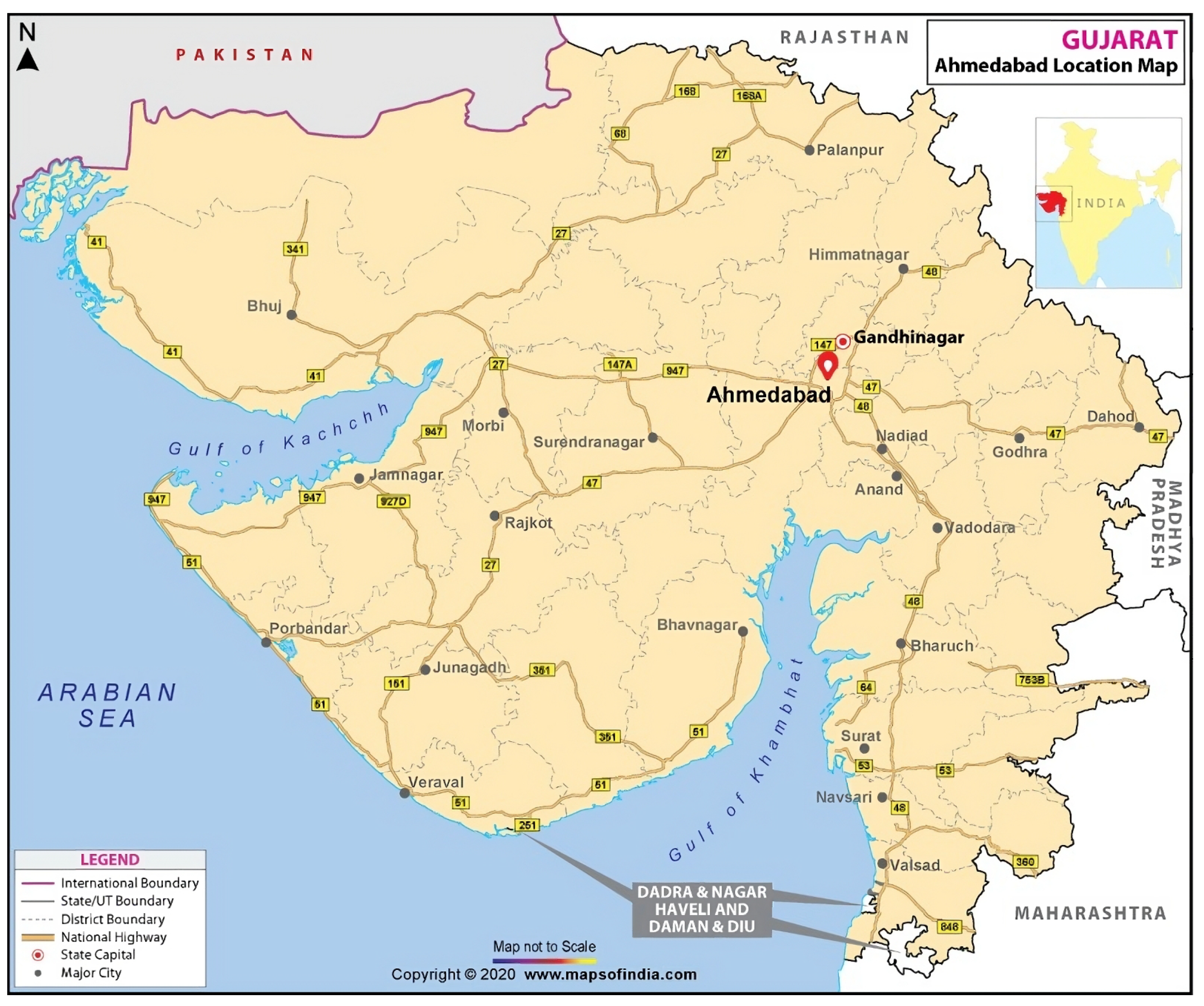
Forecasting Maximum Temperature Trends with SARIMAX: A Case Study from Ahmedabad, India

Abstract

Globalization and industrialization have significantly disturbed the environmental ecosystem, leading to critical challenges such as global warming, extreme weather events, and water scarcity. Forecasting temperature trends is crucial for enhancing the resilience and quality of life in smart sustainable cities, enabling informed decision-making and proactive urban planning. This research specifically targeted Ahmedabad city in India and employed the seasonal autoregressive integrated moving average with exogenous factors (SARIMAX) model to forecast temperatures over a ten-year horizon using two decades of real-time temperature data. The stationarity of the dataset was confirmed using an augmented Dickey–Fuller test, and the Akaike information criterion (AIC) method helped identify the optimal seasonal parameters of the model, ensuring a balance between fidelity and prediction accuracy. The model achieved an RMSE of 1.0265, indicating a high accuracy within the typical range for urban temperature forecasting. This robust measure of error underscores the model’s precision in predicting temperature deviations, which is particularly relevant for urban planning and environmental management. The findings provide city planners and policymakers with valuable insights and tools for preempting adverse environmental impacts, marking a significant step towards operational efficiency and enhanced governance in future smart urban ecosystems. Future work may extend the model’s applicability to broader geographical areas and incorporate additional environmental variables to refine predictive accuracy further.

1. Introduction

The phenomenon of climate change, primarily characterized by a significant rise in global temperatures, presents unprecedented challenges for our planet. This escalation in temperature is especially perilous in densely populated and industrial areas, where the effects of heatwaves are exacerbated by the emission of greenhouse gases. Such environmental shifts are leading to severe, multifaceted consequences. According to the National Oceanic and Atmospheric Administration (NOAA), the period from 2018 to 2020 witnessed over 3000 deaths in the United States attributable to heat-related complications [1]. Currently, urban areas, which house more than 55% of the global population—a figure projected to swell to 68% by 2050—are on the front line, facing increased risks of premature mortality and heat-induced illnesses [2].

The primary driver of global warming, human-induced greenhouse gas emissions, resulted in a 1.1 °C increase in the average global temperature over the decade spanning 2011 to 2020 [3]. This warming trend not only raises air and ocean temperatures but also signals severe implications for urban governance and infrastructure. This study was motivated by the urgent need for government agencies to fully grasp the potential consequences of rising temperatures. By anticipating these changes, local governments can implement strategic modifications to urban infrastructure, enhancing resilience, reducing environmental impacts, and safeguarding the well-being of city dwellers in an era of escalating global temperatures.

Moreover, the repercussions of increased temperatures extend beyond immediate health risks. Elevated temperatures and humidity exacerbate conditions such as eczema, psoriasis, and other dermatological disorders, due to increased perspiration. The availability of comprehensive epidemiological data is crucial for the development of effective illness-prevention strategies and treatment protocols for affected individuals. The process strips fertile land of its flora and fauna, converting it into barren deserts. India’s alarming 122% increase in land lost to forest fires within a mere five-year span illustrates the devastating synergy between high temperatures, dry conditions, and the propensity for wildfires, which in turn lead to widespread deforestation [4].

The detrimental impacts of climate change do not end at land degradation. Rising sea levels pose a direct threat to coastal communities, where approximately 40% of the global population resides. The melting of polar ice caps, coupled with the thermal expansion of ocean waters, contributes to a higher incidence of coastal erosion, elevated storm surge levels, and the enhanced severity of coastal storms [5]. Informed by the assessments of the Intergovernmental Panel on Climate Change (IPCC), governments worldwide are grappling with the task of understanding and mitigating the multifarious impacts of climate change [3].

The pivotal role of temperature projections in addressing the myriad challenges posed by climate change cannot be overstated [6]. The urgency of achieving Sustainable Development Goal 11—SDG11 (i.e., “make cities and human settlements inclusive, safe, resilient, and sustainable”) [7] underscores the importance of leveraging innovative technologies and methodologies for sustainable urban development. Accurate temperature projections have emerged as a pivotal tool in this context, enabling cities to adapt to climate change proactively, improve urban planning, and ensure the well-being of their inhabitants. The goal is not only to enhance the accuracy of temperature predictions but also to contextualize these forecasts within the broader spectrum of climate change impacts in urban areas. This endeavor underscores the critical need for interdisciplinary approaches in addressing the complex challenges posed by global warming, paving the way for innovative solutions that can protect and enhance the quality of life in urban settings across the globe [8].

More specifically, an advanced statistical forecasting model, such as the seasonal autoregressive integrated moving average with exogenous factors (SARIMAX) model, can offer promising avenues for enhancing weather forecasting accuracy. The SARIMAX model extends the capabilities of the traditional ARIMA model by incorporating both seasonal adjustments and exogenous variables. These inclusions allow the model to account for seasonal variations, which are particularly significant in meteorological data, and to incorporate external factors that influence weather patterns, such as environmental indices or economic indicators [9].

The integration of exogenous variables into the SARIMAX model enables it to capture the impact of events or inputs outside typical meteorological datasets, providing a more holistic view of the factors that affect weather conditions. For instance, in urban settings like Ahmedabad, where rapid urbanization and environmental changes play a crucial role, the SARIMAX model can utilize data on urban heat islands, pollution levels, or land-use changes as exogenous inputs [10]. This enhances the model’s accuracy in predicting temperature fluctuations and other weather-related phenomena.

The present research leveraged a decade’s worth of temperature data from Ahmedabad city in India, employing the SARIMAX model to forecast future temperature trends. Such time-series analysis-based models stand at the forefront of our efforts to predict and mitigate the adverse effects of climate change, enabling city planners and policymakers to devise informed, strategic responses to this global crisis [11]. The choice of Ahmedabad as a case study offers a unique lens through which to examine the implications of temperature forecasting in rapidly urbanizing regions. As one of India’s most populous cities, Ahmedabad embodies the challenges and opportunities inherent in managing urban growth and environmental sustainability in the face of climate change. To sum up, the current research aims to contribute to the burgeoning field of urban climate studies, providing insights that may inform the development of more resilient, adaptive urban infrastructures capable of withstanding current and future climatic shifts.

The remainder of this paper is structured to methodically unfold the research carried out, starting with Section 2 that offers a comprehensive review of existing studies, comparing various forecasting models and methodologies that have previously been employed to predict temperature changes and assess their impacts. Following this, Section 3 presents the proposed methodology, detailing the SARIMAX model’s development, the rationale behind its selection, and the specific steps taken to tailor it for temperature forecasting in Ahmedabad. Section 4 evaluates the model’s performance through rigorous testing against historical temperature data, employing statistical measures to assess its accuracy and reliability. Finally, Section 5 concludes the paper, summarizing the key findings and contributions of this study, while also highlighting potential directions for future research to further refine and expand upon the predictive capabilities of temperature forecasting models.

2. Related Work

Advancements in forecasting methodologies have significantly enriched the arsenal available for tackling the intricacies of climate variability and weather prediction. This diversification reflects a growing recognition of the multifaceted nature of weather phenomena and the critical role of accurate predictions in mitigating their impacts. The exploration of innovative forecasting models, ranging from statistical analyses to cutting-edge computational techniques, illustrates the dynamic evolution of the field [12].

An innovative approach that combined seasonal autoregression with wavelet decomposition on historical temperature data from Delhi highlighted the effectiveness of melding classical statistical tests, such as the augmented Dickey–Fuller test, with advanced data decomposition techniques [13]. This methodology not only bolstered the forecast accuracy but also set a precedent for the application of sophisticated models in climatic analysis. Concurrently, the exploration of wind speed forecasting models revealed that multivariate configurations offer superior performance over univariate models, advocating for the inclusion of multiple meteorological variables to refine predictions [14].

Neural networks, particularly Bi-LSTM (bidirectional long short-term memory) models, marked a significant breakthrough in weather forecasting, demonstrating that model training over varied temporal spans can drastically influence prediction accuracy [15]. The distinct advantage of shorter prediction intervals in improving air temperature forecasts highlights the critical role of data granularity and the model architecture in predictive performance [16]. The success of hybrid models combining genetic algorithms with LSTM networks for rainfall prediction further validated the potential of integrating machine learning techniques with evolutionary algorithms to capture complex temporal trends, offering a superior alternative to conventional models [17].

The exploration of hybrid forecasting models revealed a strategic blend of methodologies to tackle the multifaceted nature of weather prediction. The application of classifier approaches, such as Chi square and naive Bayes algorithms, demonstrated the power of statistical learning for identifying intricate patterns within historical weather data, enhancing the precision of future forecasts [18]. This narrative is complemented by studies comparing the efficacy of statistical, artificial intelligence, and hybrid models, which collectively emphasized the importance of model selection tailored to specific forecasting challenges and data characteristics [19].

Advanced statistical methods have also been applied to weather forecasting, with certain studies pointing out that semi-average methods are well-suited for scenarios involving interval or imprecise data, providing a robust framework for trend analysis in neutrosophic statistics [20]. Similarly, the employment of the Markov-chain Monte-Carlo approach alongside a seasonal autoregressive integrated moving average model for wind speed estimation underscored the utility of seasonal autoregression in achieving precise high-speed predictions. This approach also highlighted the efficacy of Markov chain Monte-Carlo methods for short-term forecasting accuracy [21].

Comparative analyses of forecasting models serve to benchmark the performance and applicability of various advanced statistical approaches, including the SARIMAX and GARCH (generalized autoregressive conditional heteroskedasticity) models. The GARCH model is particularly renowned for its ability to model financial time-series data where volatility clustering—a phenomenon where high-volatility events are followed by high-volatility events and low-volatility events are followed by low-volatility events—is observed. This makes it highly suitable for risk management and option pricing in financial markets, contrasting with SARIMAX’s utility in handling seasonal variations and external factors in meteorological and environmental data. These studies not only highlighted the significance of incorporating exogenous factors in enhancing model robustness but also underscored the relevance of these methodologies in addressing real-world problems, such as urban planning and climate change adaptation [22]. The demonstrated correlation between forecast and observed air temperatures in studies focused on specific locales further attests to the practical effectiveness of these models, validating their utility in operational settings [9].

In addition to advanced forecasting models like SARIMAX, traditional methods continue to play a crucial role in environmental and climatic studies. One such method, the Mann–Kendall trend test, is widely recognized for its robustness in detecting trends in time-series data, even with missing values or seasonal fluctuations. Originally developed for hydrological data, its application extends to a broad array of environmental sciences, providing a foundational comparison for newer methods. This test’s non-parametric nature allows it to effectively handle the non-normal datasets often encountered in climatic trend analyses [23].

The collective insights from studies such as the abovementioned underscore the dynamic and interdisciplinary pursuit of accuracy and reliability in weather forecasting. As the field gravitates towards integrating diverse models and methodologies, the emphasis on adaptability, precision, and practical application becomes increasingly evident. To conclude, the existing related works provided a foundational understanding that informed and motivated the present study, aiming to harness the strengths of the SARIMAX model for refined temperature prediction in the context of Ahmedabad city in India, thereby contributing to global research efforts in the fields of climate resilience and sustainable urban development.

3. Proposed Methodology

3.1. Data Selection

The cornerstone of our predictive analysis was a curated dataset procured from the India Meteorological Department (IMD), a repository acclaimed for its exhaustive and precise records of weather and climate data. The data were sourced directly from the Indian Meteorological Department, specifically from their Ahmedabad office. This dataset encompasses monthly maximum temperature observations for Ahmedabad, Gujarat, spanning an extensive period from January 1993 to December 2022. This selection was not arbitrary; it encapsulates a period marked by significant climatic shifts, offering a rich canvas to explore temperature trends and anomalies.

The decision to utilize monthly maximum temperature data over daily data was driven by the objective to reduce noise and short-term fluctuations, which are more prevalent in daily recordings. Monthly aggregations provide a clearer view of long-term trends and are more suitable for the strategic planning needs of urban climate management. This approach allows for a more reliable analysis of climatic patterns, which is necessary for effective policy formulation and urban planning.

The dataset is further characterized by descriptive attributes—index, year, month, and maximum temperature—comprising a comprehensive collection of 360 records across four distinct features, as elaborated in

Table 1. Features of the temperature dataset.

Feature	Description
INDEX	City Identifier
YEAR	Year of Record
MN	Month
MAX	Maximum Temperature (℃)

.

The dataset’s structure is designed to facilitate a granular analysis of temperature patterns. The index feature, identifying Ahmedabad, ensures geographical specificity, which is crucial for localized climate studies. The year and month attributes provide a temporal framework, enabling a detailed examination of seasonal dynamics and long-term climatic trends. Central to our study was the MAX feature, denoting the highest temperature recorded each month, which formed the basis of our forecasting endeavor.

This strategic selection of data grounded our research in a context that is both geographically and temporally pertinent. This ensured that our forecasting model was informed by a dataset that is not only comprehensive but also reflective of the nuanced climate dynamics specific to Ahmedabad. The period covered by the dataset, spanning three decades, is particularly significant, allowing a realistic possibility of capturing a range of climatic phenomena that could influence temperature trends, from seasonal variations to more pronounced effects of global climate change.

By anchoring our analysis in this robust dataset, we aimed to enhance the precision and relevance of our forecasting model. The geographical specificity to Ahmedabad, coupled with the dataset’s extensive temporal span, provided a solid foundation for identifying and forecasting temperature trends. It was this specific approach to data selection that underpinned the reliability and applicability of our predictive analysis, so that the insights derived are accurate enough to be actionable for addressing the challenges posed by climate variability in the region.

Ahmedabad, one of India’s most populous urban agglomerations, serves as an exemplary case study for assessing urban temperature dynamics, due to its distinct geographic and climatic conditions. Located in the western part of India, this city experiences a range of climatic variations, from intense heatwaves during summer to moderate winters, making it a critical area for studying urban heat phenomena. The city’s rapid urbanization has also led to significant environmental changes, such as increased land surface temperatures and altered local weather patterns, which are pivotal for understanding urban climate interactions.

Figure 1 illustrates the location of Ahmedabad within India. Ahmedabad has a strategic geographic position in India and is characterized by specific urban and environmental factors that made the city a significant focus of our research.

3.2. Data Preprocessing

The essence of this research lay in accurately forecasting the maximum daily temperature for the Ahmedabad city in India. A meticulous data preprocessing phase was crucial to achieving this goal, detailed as follows:

3.2.1. Data Cleaning and Transformation

Initially, the dataset underwent a thorough cleaning process to better align with the requirements of our forecasting model. The ‘Index’ column, serving only as a placeholder for “Ahmedabad”, was deemed redundant and subsequently removed. This step was followed by quality assurance checks to verify the consistency and integrity of temperature records, including outlier detection and correction to ensure data reliability.

Recognizing the periodic nature of our forecasting, a pivotal transformation involved the creation of a ‘Date’ column by merging ‘Year’ and ‘Month’ into a date–time format, which was then designated as the index. This restructured the dataset into a two-dimensional array, comprising ‘Date’ and ‘Max Temperature (MMAX)’ columns. This restructuring facilitated a more organized data analysis, directly supporting the statistical summary provided in

Table 2. Descriptive statistics of the maximum temperature for the Period 1993 to 2022.

	Mean	Standard Deviation	Min	Max
Max Temperature	34.42	4.18	26.10	43.80

, which outlines the descriptive statistics—mean, standard deviation, minimum, and maximum values—of the max temperature observed from 1993 to 2022. Such a format simplified the subsequent analyses and enhanced the clarity of our forecasting process. Although normalization and standardization processes were evaluated to facilitate model training, they were not applied in this instance, due to the model’s robustness to scale variations. These practices are typically considered where the data scale might unduly influence learning processes.

In this study, the focus was placed on the maximum temperatures, due to their critical impact on peak energy demand, heat-related health risks, and urban heat island effects, which are particularly significant in rapidly urbanizing regions like Ahmedabad. However, it is acknowledged that minimum temperatures also hold substantial meteorological and climatic importance, especially in areas experiencing significant urbanization, as they affect aspects like frost occurrence and heating needs.

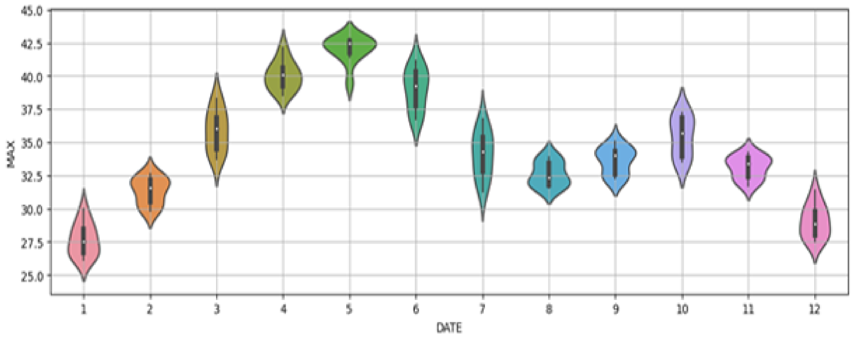
3.2.2. Observing the Trend

To illustrate the intra-annual variability and highlight potential outliers within Ahmedabad’s temperature data, we utilized a violin plot, focusing on a single year to provide a detailed view of seasonal dynamics. This is shown in Figure 2. The choice of a one-year period allows for a clear demonstration of the cyclical nature of temperature variations, which is essential for understanding broader climatic patterns in urban settings. Alongside this visual analysis, a decomposition of the time series into trend, seasonal, and residual components further dissected these patterns. Employing statistical tests like the Mann–Kendall trend test, we quantified the significance and persistence of the observed temperature trends, confirming their statistical relevance over the studied period.

3.2.3. Stationarity Check Using Augmented Dickey–Fuller Test

Ensuring data stationarity is a cornerstone of the application of the SARIMAX model in time-series forecasting. Stationary data allow the model to effectively identify and leverage meaningful patterns, relationships, and trends inherent in the dataset. Achieving stationarity, through differentiation and transformation of the data, stabilizes the model parameters, thereby bolstering the reliability and accuracy of its predictions. This foundational aspect of the SARIMAX model underscores the importnace of stationarity for the model’s operational efficacy and the trustworthiness of its forecasts. To ascertain the stationarity of our time-series data, we employed the augmented Dickey–Fuller (ADF) test, a robust method for stationarity verification [24].

The ADF test, an enhanced iteration of the original Dickey–Fuller test, is designed to assess whether a given time series exhibits stationarity. This test was imperative for our analysis; a non-stationary dataset would undermine the forecasting capability of the model, as the SARIMAX model relies on stationary data to generate forecasts. The ADF test scrutinizes the null hypothesis that a unit root is present within the time series, indicating non-stationarity [25].

The test equation is formalized as follows:

$$\Delta y_t=\alpha +\beta t+\gamma y_{t-1}+{\delta }_1\Delta y_{t-1}+\cdots +{\delta }_{p-1}\Delta y_{t-p+1}+{ϵ}_t$$

(1)

where $\Delta y_t$ represents the difference of the time series at time t, $\alpha$ is the intercept term, $\beta t$ captures the linear trend, and $\gamma$ represents the lagged level term. The coefficients ${\delta }_1$ to ${\delta }_{p-1}$ correspond to the lagged difference terms, with p denoting the number of lags and ${ϵ}_t$ being the error term, capturing the deviations not explained by the model.

The ADF test outcome hinges on the test statistic value; a value that is more negative compared to the threshold suggests a stronger likelihood of stationarity within the time series, thereby enhancing the validity of the subsequent SARIMAX forecasting [26].

3.3. Temperature Forecasting Using SARIMAX

The seasonal autoregressive integrated moving average with exogenous variables (SARIMAX) model represents an evolution of the ARIMA model, specifically designed to tackle time-series data characterized by seasonal fluctuations and the influence of external factors. This advancement allows the SARIMAX model to encapsulate complex behaviors within time-series data, which traditional ARIMA models might overlook, by incorporating exogenous variables into its predictive framework [10]. Central to the SARIMAX model is the SARIMA component, which methodically accounts for the seasonal aspects of the data. The SARIMA notation, denoted as SARIMA(p,d,q)(P,D,Q)_s, elucidates the structure of this model component, highlighting its capacity to capture both non-seasonal and seasonal dynamics within the dataset:

• p, d, and q represent the non-seasonal components of the model, indicating the order of autoregressive terms, the degree of differencing, and the order of moving average terms, respectively.
• P, D, and Q detail the seasonal elements, specifying the order of seasonal autoregressive terms, the degree of seasonal differencing, and the order of seasonal moving average terms.
• s denotes the seasonal periodicity, defining the cycle’s length within the time-series data.

3.3.1. SARIMAX

The SARIMAX (seasonal autoregressive integrated moving average with exogenous variables) model is an advanced statistical method designed for complex time-series forecasting. This method effectively integrates both seasonal adjustments and external variables, enhancing its applicability and accuracy in urban climate analysis. As part of advanced statistical methods, SARIMAX extends the capabilities of traditional time-series models by allowing for the incorporation of external influences and cyclic changes, which are crucial in understanding and predicting temperature dynamics in urban settings. The model can be succinctly expressed as follows:

$$SARIMAX(p,d,q){(P,D,Q)}_s=SARIMA(p,d,q){(P,D,Q)}_s+eXogenousvariables$$

(2)

This incorporation of exogenous variables allows the SARIMAX model to accommodate the influence of external factors, providing a more holistic approach to forecasting [27]. The components that constitute the SARIMAX model are as follows:

• Autoregressive (AR) Component: This encapsulates the influence of the preceding values on the current value, denoted as $AR\left(p\right)$, where p is the number of lag observations included in the model. The AR part is formulated as

  $$X_t=\sum _{n=1}^p{\varphi }_n{X}_{t-n}+{ϵ}_t$$

  (3)
• Integrated (I) Component: This facilitates the stationarity in the series by differencing the data, represented as $I\left(d\right)$, with d indicating the degree of differencing required.

  $$I\left(d\right)=X_t-X_{t-d}$$

  (4)
• Moving Average (MA) Component: This models the error of the time series as a linear combination of error terms from previous forecasts, expressed as $MA\left(q\right)$, where q is the order of the moving average term [28].

  $$X_t=\sum _{n=1}^q{\theta }_n{ϵ}_{t-n}+{ϵ}_t$$

  (5)
• Seasonal Components: These include Seasonal $AR\left(P\right)$ and Seasonal $MA\left(Q\right)$ terms, adding layers to capture seasonal effects within the data.
• Exogenous Variables ($Z_t$): These represent external variables influencing the time series, incorporated as additional predictors to enhance the model’s accuracy [29].

The specific settings used for the SARIMAX model parameters in our analysis were determined through extensive diagnostic testing to ensure optimal model performance:

• Parameter settings: $p=2$, $d=1$, $q=2$ for the non-seasonal components, and $P=1$, $D=1$, $Q=1$, $s=12$ for the seasonal components, tailored to capture the annual cycle evident in temperature data.
• Exogenous variables ($Z_t$): To enhance the predictive power of the SARIMAX model, we included specific climatic and economic indicators known to affect temperature variations. These exogenous variables were selected based on their relevance and data availability:

  −

  Pollution indices: Local air quality measurements such as PM2.5 and NO₂ concentrations were included, which have been shown to correlate with temperature anomalies due to their impact on atmospheric composition and heat retention.

  −

  Urban development rates: Quantified through changes in land use patterns, population density, and construction activity within the region. These metrics were sourced from municipal urban development reports and satellite imagery analysis, reflecting the urban heat island effect, which significantly impacts local temperature patterns.

  −

  Vegetation indexes: Utilizing NDVI (normalized difference vegetation index) data derived from satellite images to account for changes in land cover and their effects on the local climate. Vegetation affects local temperature through evapotranspiration and provides cooling, which can be a critical variable in urban settings.

  −

  Economic indicators: Economic growth rates and industrial activity levels, obtained from government economic reports, which indirectly affect temperature through energy consumption patterns and the resultant heat emissions.

These variables were integrated into the SARIMAX model to provide a comprehensive view of the factors influencing temperature trends, ensuring that the forecasts accounted for both direct meteorological conditions and the broader environmental and economic context.

By weaving together these components, the SARIMAX model establishes a robust framework capable of addressing the nuances of seasonal time-series data influenced by external variables:

$$X_t=AR+I+MA+SeasonalComponents+Z_t$$

(6)

where $Z_t$ represents the exogenous variables, enriching the forecasting model with additional data points that might influence the time series beyond its own historical values.

A deeper examination of the SARIMAX model’s architecture reveals its capacity to synthesize various components of time-series analysis into a single predictive framework. This synthesis is articulated through the equation:

$$X_t=\sum _{n=1}^p{\varphi }_n{X}_{t-n}+\sum _{n=1}^q{\theta }_n{ϵ}_{t-n}+{ϵ}_t+(X_t-X_{t-d})+S\left(m\right)+Z_t$$

(7)

Each term within this equation plays a pivotal role in modeling the time-series data:

• ${\varphi }_i$: These autoregressive coefficients quantify the influence of prior values within the series on the current value, embedding the model’s memory of past observations.
• ${\theta }_i$: Moving average coefficients model the impact of past errors (or shocks) on the current observation, allowing the model to adjust for anomalies or unexpected changes in the time series.
• $X_t$: Represents the actual value of the series at time t, serving as both the target for prediction and a component of the model’s calculations.
• ${ϵ}_t$: The error term at time t captures the difference between the observed values and those predicted by the model, representing the unexplained variance.
• $X_{t-d}$: Denotes the value of the series at a time lagged by d periods, essential for the model’s differencing process, aimed at achieving stationarity.
• $S\left(m\right)$: Refers to the seasonal ARMA components, which are crucial for capturing and modeling the cyclical patterns inherent in the data, ensuring that the model accurately reflects seasonal variations.
• $Z_t$: Exogenous (or external) variables are included as additional predictors to account for the influence of outside factors on the time series. These variables can significantly enhance the model’s accuracy by integrating relevant external information, such as economic indicators or environmental factors, that may impact the series.

3.3.2. Advantages and Disadvantages of SARIMAX

The SARIMAX model offers significant advantages in the field of temperature forecasting, particularly due to its ability to integrate seasonal patterns and exogenous variables into the forecasting process. This integration allows for enhanced accuracy and applicability in urban settings, where external factors such as urban development and environmental policies play a crucial role in temperature dynamics. The flexibility in model tuning also allows for adaptations to specific local conditions, making it a robust tool for climate-sensitive planning.

However, the model is not without its challenges. The complexity of setting up a SARIMAX model, due to the need to identify correct parameters and integrate external data, can be a significant barrier. Additionally, the model’s effectiveness is heavily dependent on the availability of comprehensive and high-quality historical data. Computational resources can also be a constraint, as the model may require significant processing power for large datasets or complex variable integrations.

These factors must be carefully considered when choosing the SARIMAX model for urban temperature forecasting projects, to ensure that the benefits outweigh the potential difficulties.

3.3.3. Seasonal Hyperparameter Tuning Using AIC

The Akaike information criterion (AIC) is a mathematical technique employed to determine the fit of a model to the data it is derived from. It is instrumental in estimating the optimal values of both ARIMA and seasonal parameters (p, d, q) (P, D, Q), ensuring the model is well-fitted without being overfitted. A lower AIC value is indicative of a model that better fits the data [30]. The AIC is computed based on the number of independent variables K used to construct the model and its capacity to replicate the observed data.

A model achieving a high explanatory power with the fewest independent variables is considered optimal. When comparing models that account for a similar amount of variability, the model with fewer parameters—and, consequently, a lower AIC score—is preferred [31,32]. This approach facilitates a comparative evaluation of model quality rather than an absolute measure.

The AIC for a model is calculated using the following equation:

$$AIC=-2\times (log-likelihood)+2K$$

(8)

where the $log-likelihood$ component assesses the model’s fit to the data, with higher values indicating a better fit. The term $2K$, where K is the number of model parameters, penalizes complexity, discouraging the overfitting that can come from models with excessive parameters.

In the context of the SARIMAX model, the AIC serves a pivotal role in determining the optimal set of parameters—both the ARIMA (p, d, q) and the seasonal (P, D, Q) components. By iterating over possible combinations of these parameters and calculating the AIC for each, the model selection process gravitates towards configurations that offer a judicious blend of predictive accuracy and model parsimony. A lower AIC value signifies a model that has achieved a commendable fit to the data without resorting to unnecessary complexity. This principle of parsimony is crucial, especially in the domain of time-series forecasting, where the temptation to “overfit” to historical data can detract from a model’s predictive power in unseen scenarios.

The deliberate tuning of SARIMAX parameters guided by the AIC thus represents a methodical approach to enhancing forecasting performance. It is a process of refinement, where the ultimate goal is not just to fit the historical data as closely as possible but to construct a model that generalizes well to future data points. This approach underlines the essence of forecasting as a forward-looking endeavor, where the true measure of a model’s value lies in its ability to anticipate future trends with clarity and confidence.

In summary, the AIC’s role in SARIMAX modeling transcends mere numerical evaluation. It embodies a principle of modeling efficiency that is crucial for predictive analytics. By steering the model selection process towards configurations that offer an optimal balance between accuracy and simplicity, AIC-guided hyperparameter tuning enhances the reliability and robustness of temperature forecasts. This methodological rigor ensures that the SARIMAX model, with its nuanced understanding of seasonal patterns and external influences, stands as a formidable tool in the arsenal of climate prediction and analysis methods.

3.4. Proposed Algorithm

The endeavor to forecast temperature with high accuracy is critical across various sectors, impacting everything from agricultural productivity to urban climate management. The complex interplay of factors affecting atmospheric conditions necessitates a sophisticated approach to model development. Our proposed methodology leverages the SARIMAX model, an advanced iteration of time-series forecasting models, to capture the nuanced effects of seasonality and external variables on temperature trends. Algorithm 1 embodies a structured pathway from data acquisition to comprehensive model evaluation, aimed at predicting the monthly average maximum temperature in Ahmedabad with unprecedented precision.

This algorithm represents a strategic synthesis of statistical techniques and model optimization processes designed to fine-tune the forecasting model for maximal accuracy. The forecasting objective, delineated as $T_{\mathrm{pred}}$, encompasses a comprehensive set of monthly temperature projections that are instrumental for both immediate response and long-term strategic planning in various sectors affected by climate variability.

$$T_{\mathrm{pred}}=\{T_{m1},T_{m2},\dots ,T_{m12}\}$$

(9)

where $T_{\mathrm{pred}}$ embodies the forecast monthly average temperatures, each element corresponding to a month’s projection, predicated through the analysis of temperature patterns over the preceding decade. This predictive endeavor harnesses the SARIMAX model’s capability to dissect and model temperature trends, factoring in both inherent seasonal shifts and the impact of exogenous variables.

Algorithm 1 Forecasting monthly average maximum temperature using SARIMAX

1: Collect the dataset from the India Meteorological Department (IMD), ensuring a rich and reliable foundation for analysis. 2: Pre-process the data, tailoring them to meet the specific needs of the SARIMAX model. This includes cleaning, normalization, and preparation of time-series data. 3: Conduct a stationarity check using the augmented Dickey–Fuller test, a critical step to validate the time series’ suitability for SARIMAX modeling. 4: if p-value < 0.05 then 5:   Accept the null hypothesis (data are stationary) 6: else 7:   Perform differencing and return to stationarity check 8: end if 9: Apply the statistical time-series-based model (SARIMAX) 10: Use the auto-ARIMA model to determine optimal $(p,d,q)$ and $(P,D,Q)$ based on AIC value 11: Forecast the temperature for the required year using data from the previous 10 years 12: Evaluate the performance using MSE, RMSE, $R^2$, and MAE

The SARIMAX model stands out for its integrative approach, accommodating the complex dynamics of temperature data through its multifaceted components. By conducting rigorous data preprocessing and ensuring data stationarity, the model builds on a solid analytical foundation. The strategic application of auto-ARIMA for parameter selection—guided by the principle of minimizing the AIC—reflects a commitment to model efficiency and accuracy.

Evaluating the model’s performance through established metrics allowed for a nuanced understanding of its predictive capacity, highlighting areas of strength and potential for further refinement. This meticulous process not only enhanced the reliability of the temperature forecasts for Ahmedabad but also sets a precedent for the application of the SARIMAX model in broader climatological research and operational forecasting.

To sum up, the proposed algorithm encapsulates a comprehensive, methodically structured approach to temperature forecasting. It underscores the SARIMAX model’s adaptability and effectiveness in capturing the intricate patterns of temperature variability, offering valuable insights for future research and practical applications in temperature forecasting. This detailed exposition aimed to elucidate the algorithm’s components and their collective role in advancing the precision and applicability of temperature predictions.

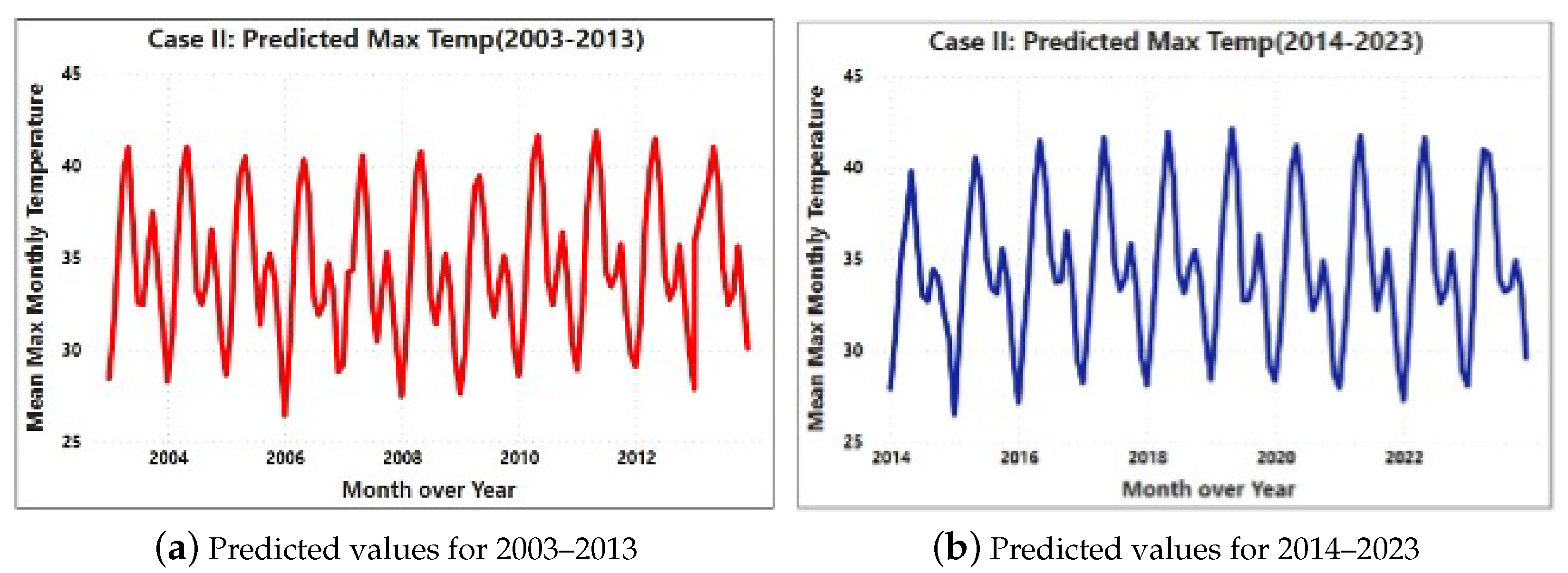
3.4.1. Case 1: Initial Forecasting Approach

Our initial foray into forecasting Ahmedabad’s temperature patterns commenced with an auto-ARIMA-driven analysis. Auto-ARIMA, an automated version of the ARIMA model selection process, scans through a predefined range of model parameters—(p, d, q) for the autoregressive, differencing, and moving average components, respectively, and (P, D, Q) for their seasonal counterparts. The goal was to pinpoint the optimal set of parameters that minimized the Akaike information criterion (AIC), a statistical measure used to compare models by balancing goodness of fit with model complexity.

The SARIMAX model, enhanced with the selected parameters, underwent rigorous training. This phase was crucial for assimilating the temporal and seasonal dynamics encapsulated in the dataset, covering a decade of temperature observations. The model’s predictive accuracy was initially promising, demonstrating a high degree of alignment with actual temperature data for up to three years post-training. However, the model’s performance began to diverge as the predictions extended further into the future. This deviation was attributed to the model’s reliance on cumulative historical data, where each year’s forecast values were integrated back into the dataset for future predictions. Such a methodology inadvertently magnified the margin of error with each successive forecast. These compounded inaccuracies highlighted a fundamental challenge in long-term forecasting: the inherent difficulty of maintaining accuracy over extended periods, especially in the face of fluctuating climate variables and potential shifts in underlying environmental patterns [33].

The escalating forecast uncertainty was illustrated by the broadening error margins observed across the different forecast periods. Initially, the model maintained an error range from −4 °C to 4 °C, which significantly widened to −8 °C to 8 °C as the forecasting horizon moved from the period of 2003 to 2012, to 2013 to 2023. These findings suggest that, while the auto-ARIMA-driven SARIMAX model exhibited robust short- to medium-term forecasting capabilities, its long-term reliability diminished due to accumulating forecast errors and the dynamic nature of climatic conditions.

The insights derived from Case 1 underscored the necessity for adaptive forecasting strategies capable of accommodating evolving climatic patterns and mitigating the accumulation of predictive errors. Periodic recalibration of model parameters, informed by continuous data monitoring and validation against emerging climatic trends, may serve as a vital approach for sustaining forecast accuracy over extended periods. Moreover, exploring alternative forecasting models or hybrid approaches that can dynamically adjust to new data inputs and unforeseen environmental variables may offer pathways to enhance the robustness and reliability of long-term temperature forecasts.

In summary, the initial forecasting approach provided a valuable foundation for understanding the operational strengths and limitations of employing auto-ARIMA for SARIMAX model parameter selection. The lessons learned paved the way for developing more resilient forecasting methodologies that can effectively navigate the complexities of long-term climate prediction, ensuring that models remain pertinent and accurate in the face of an ever-changing environmental landscape.

3.4.2. Case 2: Dynamic Forecasting Strategy

Our exploration in Case 2 pioneered a dynamic and iterative forecasting strategy, leveraging a rich temporal dataset spanning from 1993 to 2022 for Ahmedabad. This method started with the model being trained on the initial decade’s data, aiming to predict the subsequent year’s temperatures. Significantly, this procedure was iterative; it involved progressively advancing the training window by one year at each step, thereby ensuring that the model was continuously refreshed with the most recent data, enhancing its predictive accuracy over time.

One of the cornerstone decisions in this methodology was the intentional exclusion of forecast values from the subsequent training sets. This strategic choice was predicated on the understanding that forecast values, while informative, inherently possess a degree of uncertainty. By relying exclusively on observed data for model training, we ensured that the integrity and accuracy of the forecasting process were preserved, anchoring the model’s predictions in empirical evidence. The adoption of a rolling-window training approach underpinned the model’s robustness and adaptability. This methodology ensured that the model was not only perpetually updated with the latest data but also rigorously tested against diverse data subsets. This reflective approach closely mirrored real-world forecasting conditions, thereby enhancing the model’s ability to adapt to evolving climatic patterns and improving its generalization capability over an extended temporal horizon.

The efficacy of the dynamic forecasting strategy was demonstrated through the display of predicted monthly maximum temperatures for two distinct periods, 2003–2013 and 2014–2023, as depicted in Figure 3a,b. These visualizations underscore the model’s capacity to consistently generate predictions that reflect potential temporal shifts in climate patterns. This representation affirms the model’s utility in forecasting climate trends, highlighting its ability to effectively adapt and predict future climatic conditions, which is crucial for strategic planning in urban climate management.

The unfolding of Case 2 showcased not just a methodological advancement in temperature prediction but also a paradigmatic shift towards a more adaptive and responsive forecasting framework. This strategy exemplified the imperative for climate models to be dynamic and capable of evolving in tandem with their datasets, to maintain relevance and accuracy in an ever-changing environmental landscape.

Looking ahead, the implications of this approach are profound, offering a blueprint for further enhancing the forecasting model. The potential integration of cutting-edge machine learning algorithms or the inclusion of a broader array of climatic and environmental variables could substantially refine predictive capabilities. Furthermore, the successful application of this method to different geographical regions or varying climatic phenomena opens new avenues for research and innovation in global climate prediction, underscoring the pivotal role of adaptability and iterative learning in advancing our understanding and management of climate variability.

3.4.3. Comparative Analysis of Case 1 and Case 2

In the comparative analysis between Case 1 and Case 2, we delve into the nuances that delineated their distinct forecasting strategies and outcomes. Case 1 leveraged an auto-ARIMA function to deduce optimal SARIMAX model parameters, with a strategy focused on minimizing the Akaike information criterion (AIC) for enhanced model accuracy in the short to medium term. Initially, this methodology demonstrated promising forecast precision, aligning closely with the actual data for the initial years following model training. However, the predictive accuracy began to diverge as the forecasting horizon extended, revealing a fundamental limitation associated with the model’s dependency on historical data. This reliance initiated an error accumulation process, which, compounded by unforeseen climatic events and shifts in environmental patterns, resulted in a significant expansion of the error range over time.

Contrasting sharply with Case 1, Case 2 adopted a dynamic and iterative forecasting strategy through a rolling-window training approach. This method, covering nearly three decades of data, continuously adapted to evolving patterns, significantly enhancing the model’s predictive accuracy and generalization capability across a prolonged timeframe. A pivotal decision in this strategy was to eschew the inclusion of predicted values in the training dataset for subsequent iterations, a move designed to prevent the snowballing of forecast errors. This approach, augmented by rigorous evaluation metrics, not only showcased a robust capacity for model adaptation but also maintained the forecasts’ empirical grounding, thus ensuring the model’s long-term predictive reliability.

Graphical representations of forecast versus actual temperatures for distinct periods further elucidate the comparative strengths of the models employed in both cases. The fidelity of Case 2’s forecasts to actual climatic outcomes, across extended time frames, accentuated its methodological superiority in capturing and adapting to temporal climatic trends. This alignment, or its absence, constituted a critical evaluation metric of the model’s efficacy, highlighting areas for potential refinement to further optimize forecasting accuracy.

The juxtaposition of Case 1 and Case 2 elucidates a broader narrative within climate forecasting: the imperative for methodologies that not only yield immediate accuracy but also sustain adaptability over time. Case 2’s rolling-window approach embodies this principle, offering a scalable and flexible framework capable of navigating the complexities of climate prediction with enhanced precision. This comparative analysis not only advances our understanding of the forecasting models’ operational dynamics but also underscores the strategic importance of methodological adaptability in the face of climatic unpredictability.

4. Experimental Evaluation

4.1. Results

In our quest to assess the precision of our monthly average maximum temperature predictions, we employed a suite of metrics to evaluate model performance across three decades [34,35]. The accuracy of the forecasts was quantified using key indicators such as Root Mean Squared Error (RMSE), Mean Squared Error (MSE), Mean Absolute Error (MAE), and the R-squared (R²) score, as illustrated in the following equations:

$$\mathrm{RMSE}\left(T\right)=\sqrt{{\displaystyle \frac{1}{m}}\sum _{i=1}^m{(g_i-{\widehat{g}}_i)}^2}$$

(10)

$$\mathrm{MSE}\left(T\right)={\displaystyle \frac{1}{m}}\sum _{i=1}^m{(g_i-{\widehat{g}}_i)}^2$$

(11)

$$\mathrm{MAE}\left(T\right)={\displaystyle \frac{1}{m}}\sum _{i=1}^m\left|g_i-{\widehat{g}}_i\right|$$

(12)

$$R^2\left(T\right)={\displaystyle \frac{{\sum }_{i=1}^m{(g_i-{\widehat{g}}_i)}^2}{{\sum }_{i=1}^m{(g_i-\overline{g})}^2}}$$

(13)

where T represents the year, i the month, $g_i$ the actual temperature, ${\widehat{g}}_i$ the predicted temperature, and $\overline{g}$ the average of actual temperatures. This methodology ensured a rigorous assessment of the forecasting model’s effectiveness over an extended period.

The RMSE values for the forecast years from 2003 to 2013, as presented in

Table 3. Error values for predicted years (2003–2013) from Case 2.

Year Used for Training	Predicted Year	RMSE
1992–2002	2003	1.4185
1993–2003	2004	1.5347
1994–2004	2005	1.4740
1995–2005	2006	1.5436
1996–2006	2007	1.3115
1997–2007	2008	1.0265
1998–2008	2009	1.7331
1999–2009	2010	1.4287
2000–2010	2011	1.1369
2001–2011	2012	1.1474
2002–2012	2013	1.3161

, demonstrate the performance of the dynamic forecasting strategy employed in Case 2. This table offers insights into the temporal reliability and the adaptability of our forecasting model over a decade.

Following Table 3, it is crucial to highlight the variations in the RMSE values across different forecast years, which reflect the model’s fluctuating accuracy over time. This variability is indicative of the model’s sensitivity to different training intervals and the inherent dynamics within the data. Notably, the lowest RMSE of 1.0265 in the year 2008 suggests the optimal alignment of the model parameters with the climatic patterns for that period, potentially influenced by specific environmental or economic events that year. Conversely, higher RMSE values, such as 1.7331 in 2009, point to challenges the model faced due to possible abrupt changes in climatic conditions or anomalies not captured within the training data. These results underscore the need for continuous refinement of the forecasting model, including possible adjustments in the SARIMAX model parameters or the inclusion of additional data points, to enhance predictive accuracy and reliability in varying temporal contexts. This detailed analysis helps in understanding the critical role of adaptive model tuning and robust validation practices in maintaining high forecasting accuracy over extended periods.

An in-depth analysis of these values indicated a significant correlation between predicted and actual temperatures, suggesting a high predictive accuracy. This is further affirmed by a refined equation:

$$t_{\mathrm{actual}}=t_{\mathrm{pred}}+(M\pm \delta t)$$

(14)

where M is a constant value determined to be 1, indicating a systematic underestimation by the model, and $\delta t$ represents a minor deviation in temperature, ranging between 0.1 and 0.9. This equation acknowledges a consistent bias in the model’s forecasts, suggesting that, despite the low error magnitude (with RMSE values hovering around 1), there was a predictable deviation from actual temperature values.

The identification of this systematic bias is crucial for further model refinement. Understanding the nature of this bias and exploring avenues for adjustment—be it through calibration of the model’s coefficients or the incorporation of additional predictive variables—could significantly enhance the model’s accuracy. Such enhancements aim to better capture the complex dynamics underlying temperature variations, thereby improving the reliability and applicability of the model’s forecasts in real-world scenarios [36].

4.2. Comparative Performance Analysis of Forecasting Models

This subsection provides a comparative analysis with forecasting models from the recent literature, juxtaposing them against the advancements introduced by the SARIMAX model with hyperparameter tuning in this study. The comparative lens primarily focused on RMSE, a universally recognized metric for evaluating the accuracy of predictions across various time-series forecasting challenges, including temperature prediction.

The WD-SARIMAX (wavelet decomposition-seasonal autoregressive integrated moving average with exogenous variables) model is a hybrid forecasting approach that first applies wavelet decomposition to the time-series data. This decomposition separates the time series into various frequency components, enabling the SARIMAX model to handle these components separately, thus improving the accuracy and robustness of the forecasts.

The WD-SARIMAX method delivered an RMSE score of 1.67 for temperature prediction tasks [13]. This stands in contrast to the refined SARIMAX model proposed in our study, which integrated meticulous hyperparameter tuning aimed at optimizing the model’s performance. The effectiveness of this enhancement was evidenced by an improved RMSE value of 1.026, underscoring the potential of hyperparameter optimization for elevating forecasting accuracy.

Temperature forecasting utilizing the bi-directional LSTM model yielded an RMSE value of 1.74 [16]. This approach did not account for the stationarity of the data, a critical factor in time-series analysis. Conversely, our methodology incorporated the augmented Dickey–Fuller test for stationarity verification, combined with targeted fine-tuning of the model parameters. This strategic adjustment not only improved the computational efficiency but also notably refined the RMSE to 1.026, affirming the importance of data pre-processing in enhancing model precision.

In [22], the SARIMAX model was augmented with external regressors for daily demand forecasting in a hotel context, trained on a dataset covering five years. An interesting revelation from this approach was the identification of non-seasonality through the augmented Dickey–Fuller (ADF) test, challenging the typical expectation of seasonal patterns in such data. The resultant RMSE of 10.365 starkly contrasted with the outcomes from temperature forecasting, highlighting the divergent nature of data characteristics and forecasting objectives across different domains.

The application of the SARIMA model alongside the Markov chain Monte Carlo (MCMC) method for wind energy forecasting showcased an average RMSE of 16.44%, predicated on a relatively small dataset of 550 values [37]. The limitation imposed by the dataset size underscores the necessity for ample data in effectively capturing seasonal trends. While MCMC offers enhanced precision for long-range quantitative forecasts, its applicability to temperature forecasting may be constrained by the inherent differences in the nature of the data and prediction objectives.

As we delve into the comparative analysis of various forecasting methodologies, it is pivotal to contextualize the performance of each approach within the framework of predictive accuracy.

Table 4. Comprehensive comparative analysis of forecasting models.

Paper	Methodology	RMSE
[13]	WD-SARIMAX for Temperature Prediction	1.67
[16]	Bi-directional LSTM for Temperature Forecasting	1.74
[21]	Wind Energy Analysis with SARIMA and MCMC	14.66
[22]	Demand Forecasting with SARIMAX	10.365
[9]	Temperature Forecasting with Mann-Kendall and ARIMA	1.40
[24]	Weather Forecasting using Artificial Neural Network	2.55
	Proposed SARIMAX Methodology	1.026

succinctly summarizes the RMSE values obtained with the different methods, including the WD-SARIMAX, Bi-directional LSTM, and SARIMAX with external regressors models, among others. This table not only highlights the diversity of techniques applied in the forecasting challenges but also underscores the proposed SARIMAX methodology’s standout performance. By scrutinizing these RMSE scores, we can glean insights into the efficacy of hyperparameter tuning and data preprocessing, which are instrumental in the proposed method’s enhanced accuracy.

Following Table 4, we provide a detailed analysis that compares the results of the current study with those of previous studies. This analysis not only highlights the numerical differences in RMSE scores but also discusses the methodological nuances that contributed to these differences. For instance, the lower RMSE value achieved by the proposed SARIMAX methodology reflects the impact of integrating exogenous variables and hyperparameter tuning, which are not typically employed in traditional forecasting models like the Mann–Kendall and ARIMA methods used in other studies. By offering this comparison, we underscore the advancements in forecasting accuracy made possible through the innovative use of the SARIMAX model in addressing the complex dynamics of urban temperature variations. This discussion serves to contextualize the superiority of the proposed model in terms of both methodological rigor and practical outcomes, reinforcing the relevance and application of our findings in urban climate management.

The comparative analysis elucidates the nuanced performance landscape of the various forecasting models, emphasizing the significant strides made by the proposed SARIMAX methodology in achieving superior RMSE values. This benchmarking not only highlights the efficacy of incorporating hyperparameter tuning and data stationarity checks but also positions the proposed model as a robust tool for precise temperature forecasting, setting a new standard for future research and application in the field. In conclusion, by demystifying complex climate data, the proposed model can inform public awareness initiatives and foster participatory approaches in urban environmental management, ensuring that sustainable development is a shared vision.

4.3. Discussion

The experimental evaluation and comparative analysis conducted in this study have effectively demonstrated the enhanced precision of the SARIMAX methodology in forecasting monthly average maximum temperatures. The methodological rigor, characterized by meticulous integration of hyperparameter tuning and the incorporation of stationarity checks via the augmented Dickey–Fuller test, was pivotal in achieving a superior RMSE score of 1.026. This score notably surpassed those obtained from other comparative forecasting models, underscoring the robustness of our approach.

A critical insight from our analysis was the systematic underestimation identified in the predictive model. This consistent bias, marked by the deviation captured in the refined predictive equation, suggests potential areas for model enhancement. Adjusting model parameters or integrating additional climatic variables could provide a more nuanced understanding of extreme weather events and the gradual impacts of climate change on temperature patterns. This approach would not only refine the accuracy of our forecasts but also extend their applicability in climate-sensitive planning and decision-making processes.

Moreover, the variability in RMSE scores across the different models and applications—from straightforward temperature forecasting to complex energy demand predictions—highlights the multifaceted challenges inherent in time-series forecasting. These challenges are amplified by the critical role that dataset characteristics play, particularly size and seasonality, which significantly influence model performance. This observation suggests a need for sophisticated data management strategies that can effectively handle the complexities introduced by diverse data characteristics, enhancing the generalizability and reliability of forecasting models.

Additionally, the observed performance of our proposed methodology in the context of temperature forecasting has promising implications for its applicability across a broader spectrum of time-series prediction tasks. While the current study focused on temperature data, the techniques employed could be adapted to other domains, such as hydrology or energy consumption, where accurate forecasting could significantly impact resource management and policy formulation.

Despite the successes outlined, our findings also underscore the necessity for continuous model refinement. The field of predictive modeling is dynamically evolving, with new methodologies and technologies continually emerging. As such, ongoing research should aim to integrate emerging techniques, such as machine learning and artificial intelligence, to enhance the predictive capabilities of models like SARIMAX further. These advancements could facilitate more accurate, timely, and actionable forecasts, vital for managing the impacts of climate variability and change.

In summary, this discussion around the proposed SARIMAX model not only reaffirms its efficacy in forecasting but also opens avenues for substantial methodological improvements. By further exploring the integration of additional predictive variables and refining model parameters, future research could better capture the complex dynamics underlying temperature variations, thereby improving the reliability and applicability of forecasts in real-world scenarios.

5. Conclusions and Future Work

This research has significantly advanced the field of temperature forecasting by developing a sophisticated SARIMAX model, meticulously tailored to capture the unique climatic nuances of Ahmedabad. The model’s adaptability and precision in forecasting monthly average maximum temperatures were evident, as demonstrated by an impressive Root Mean Squared Error (RMSE) of 1.026. This metric not only attests to the model’s high accuracy but also underscores its potential utility in environmental planning and policy-making. Accurate temperature forecasts provide decision-makers and policymakers with critical insights, enabling the development and implementation of strategies aimed at mitigating the adverse effects of climate change. This, in turn, supports environmental sustainability initiatives and enhances community well-being in urban settings.

This study also emphasized the importance of integrating advanced statistical techniques and rigorous hyperparameter optimization to improve forecasting accuracy. The application of the augmented Dickey–Fuller test, which confirmed the stationarity of the dataset, highlighted the model’s methodological robustness and ensures the reliability of its predictive capabilities. By achieving a balance between model fidelity and predictive accuracy, this study presents a robust framework for future forecasting endeavors. Furthermore, the deliberate incorporation of both seasonal adjustments and exogenous variables allows the model to account for a wider range of influencing factors, making it a comprehensive tool for urban climate analysis.

As we look towards the horizon of temperature forecasting, several avenues emerge for refining the SARIMAX model and broadening the scope of the current research work. A deeper analysis of seasonal patterns and extreme weather events is paramount. By dissecting these temporal fluctuations with greater precision, we could uncover intricate climatic behaviors that the current model may overlook. Enhancing the model’s sensitivity to such nuances promises not only to sharpen its forecasting accuracy but also to provide a richer understanding of climate dynamics over time. Furthermore, the inclusion of additional environmental variables—ranging from humidity and precipitation to pollution levels—into the forecasting model could yield a more comprehensive framework for understanding temperature variations [38,39]. This holistic approach would allow for a more nuanced analysis of the multifaceted influences on climate, facilitating more accurate and meaningful predictions.

Exploring alternative forecasting methodologies represents another fruitful direction. The integration of machine learning algorithms or ensemble models could introduce new dimensions to temperature prediction, potentially offering improvements in both accuracy and efficiency. Such investigative efforts would contribute to a diverse toolkit for climatologists and data scientists, enabling them to select the most appropriate techniques based on the specific challenges and data characteristics at hand. Expanding the geographical scope of the SARIMAX model to encompass various cities, regions, and climatic zones would be another critical step forward. This expansion would not only validate the model’s adaptability but also pave the way for the development of localized models that cater to the distinct climatic conditions across different parts of the world. Such region-specific models could significantly enhance the accuracy of local weather forecasts, providing valuable insights for regional planning and disaster management.

Incorporating mechanisms for dynamic model updating based on real-time data streams could dramatically improve the model’s adaptability to changing weather conditions. This approach would ensure that the forecasting model remains relevant and reliable, even as rapid environmental changes occur [33]. By continuously updating its parameters in response to the latest data, the model could offer more accurate predictions, adjusting swiftly to unforeseen climatic shifts. Embarking on all these paths of inquiry and development, we aim to fortify the foundations of temperature forecasting. The ultimate goal is to harness advanced predictive analytics to better prepare for and mitigate the impacts of climate variability, ensuring a sustainable and resilient future for communities worldwide.

Our research could be further extended by incorporating traditional trend analysis methods such as the Mann–Kendall trend test alongside the SARIMAX model. Future studies could explore comparative analyses between these traditional non-parametric tests and the more complex SARIMAX approach, especially in their ability to handle datasets with non-normal distributions and missing data. Such comparative studies would not only validate the findings from SARIMAX models but also potentially uncover nuanced insights into the dynamics of climatic changes over extensive periods. Integrating these methodologies could enhance our understanding of trend behaviors across different environmental datasets.

From a broad perspective, the current research contributes to the global agenda of achieving SDG11 by highlighting how sophisticated temperature forecasting can support the sustainable management of urban landscapes. Looking ahead, integrating the proposed approach with cutting-edge technologies such as artificial intelligence, geospatial analysis, and the metaverse opens new avenues for creating resilient, adaptive, and smart urban environments. Future research will explore these integrations, aiming to provide comprehensive solutions for the multifaceted challenges of sustainable urban development.

References

- National Oceanic and Atmospheric Administration: Excessive Heat, a `Silent Killer’. Available online: https://www.noaa.gov/stories/excessive-heat-silent-killer (accessed on 16 July 2024).
- Gustin, M.; McLeod, R.S.; Lomas, K.J. Forecasting Indoor Temperatures during Heatwaves using Time Series Models. Build. Environ. 2018, 143, 727–739. [Google Scholar] [CrossRef]
- The Intergovernmental Panel on Climate Change (IPCC). Available online: https://www.ipcc.ch/report/ar6/wg1/downloads/report/IPCC_AR6_WGI_SPM_final.pdf (accessed on 16 July 2024).
- Data Dive: Land Lost to Forest Fires in India Increases by 122% in 5 Years. Available online: https://www.factchecker.in/data-dive/data-dive-land-lost-to-forest-fires-in-india-increases-by-122-in-5-years-815025 (accessed on 16 July 2024).
- The Climate Action Button. Available online: https://climatebutton.ucsusa.org/ (accessed on 16 July 2024).
- Kreuzer, D.; Munz, M.; Schlüter, S. Short-Term Temperature Forecasts using a Convolutional Neural Network—An application to Different Weather Stations in Germany. Mach. Learn. Appl. 2020, 2, 100007. [Google Scholar] [CrossRef]
- Sustainable Development Goals: 17 Goals to Transform Our World—Ensure Access to Affordable, Reliable, Sustainable and Modern Energy. Available online: https://www.un.org/sustainabledevelopment/energy/ (accessed on 16 July 2024).
- Veeramsetty, V.; Kiran, P.; Sushma, M.; Salkuti, S.R. Weather Forecasting Using Radial Basis Function Neural Network in Warangal, India. Urban Sci. 2023, 7, 68. [Google Scholar] [CrossRef]
- Kaur, B.; Kaur, N.; Gill, K.K.; Singh, J.; Bhan, S.C.; Saha, S. Forecasting Mean Monthly Maximum and Minimum Air Temperature of Jalandhar District of Punjab, India using Seasonal ARIMA Model. J. Agrometeorol. 2022, 24, 42–49. [Google Scholar]
- Brown, G.D.; Largey, A.; McMullan, C.; Reilly, N.; Sahdev, M. Weathering the Storm: Developing a User-centric Weather Forecast and Warning System for Ireland. Int. J. Disaster Risk Reduct. 2023, 91, 103687. [Google Scholar] [CrossRef]
- Zhou, H.; Zhang, S.; Peng, J.; Zhang, S.; Li, J.; Xiong, H.; Zhang, W. Informer: Beyond Efficient Transformer for Long Sequence Time-Series Forecasting. In Proceedings of the 35th AAAI Conference on Artificial Intelligence (AAAI), Virtually, 2–9 February 2021; AAAI Press: Washington, DC, USA, 2021; pp. 11106–11115. [Google Scholar]
- Roy, D.S. Forecasting The Air Temperature at a Weather Station Using Deep Neural Networks. Procedia Comput. Sci. 2020, 178, 38–46. [Google Scholar] [CrossRef]
- Elshewey, A.M.; Shams, M.Y.; Elhady, A.M.; Shohieb, S.M.; Abdelhamid, A.A.; Ibrahim, A.; Tarek, Z. A Novel WD-SARIMAX Model for Temperature Forecasting Using Daily Delhi Climate Dataset. Sustainability 2022, 15, 757. [Google Scholar] [CrossRef]
- Cadenas, E.; Rivera, W.; Campos-Amezcua, R.; Heard, C. Wind Speed Prediction Using a Univariate ARIMA Model and a Multivariate NARX Model. Energies 2016, 9, 109. [Google Scholar] [CrossRef]
- Hewage, P.; Trovati, M.; Pereira, E.; Behera, A. Deep Learning-based Effective Fine-grained Weather Forecasting Model. Pattern Anal. Appl. 2021, 24, 343–366. [Google Scholar] [CrossRef]
- Zenkner, G.; Navarro-Martinez, S. A Flexible and Lightweight Deep Learning Weather Forecasting Model. Appl. Intell. 2023, 53, 24991–25002. [Google Scholar] [CrossRef]
- Thakur, N.; Karmakar, S.; Soni, S. Time Series Forecasting for Uni-variant Data using Hybrid GA-OLSTM Model and Performance Evaluations. Int. J. Inf. Technol. 2022, 14, 1961–1966. [Google Scholar] [CrossRef]
- Biswas, M.; Dhoom, T.; Barua, S. Weather Forecast Prediction: An Integrated Approach for Analyzing and Measuring Weather Data. Int. J. Comput. Appl. 2018, 182, 20–24. [Google Scholar] [CrossRef]
- U, J.K.; Kovoor, B.C. Deterministic Weather Forecasting Models based on Intelligent Predictors: A Survey. J. King Saud Univ.—Comput. Inf. Sci. 2022, 34, 3393–3412. [Google Scholar]
- Aslam, M. Time Series Data Analysis under Indeterminacy. J. Big Data 2023, 10, 126. [Google Scholar] [CrossRef]
- Al-Duais, F.S.; Al-Sharpi, R.S. A Unique Markov Chain Monte Carlo Method for Forecasting Wind Power Utilizing Time Series Model. Alex. Eng. J. 2023, 74, 51–63. [Google Scholar] [CrossRef]
- Ampountolas, A. Modeling and Forecasting Daily Hotel Demand: A Comparison Based on SARIMAX, Neural Networks, and GARCH Models. Forecasting 2021, 3, 580–595. [Google Scholar] [CrossRef]
- Hamed, K.H.; Rao, A.R. A Modified Mann-Kendall Trend Test for Autocorrelated Data. J. Hydrol. 1998, 204, 182–196. [Google Scholar] [CrossRef]
- Abhishek, K.; Singh, M.; Ghosh, S.; Anand, A. Weather Forecasting Model using Artificial Neural Network. Procedia Technol. 2012, 4, 311–318. [Google Scholar] [CrossRef]
- Ajewole, K.P.; Adejuwon, S.O.; Jemilohun, V.G. Test for Stationarity on Inflation Rates in Nigeria using Augmented Dickey Fuller Test and Phillips-Persons Test. IOSR J. Math. 2020, 16, 11–14. [Google Scholar]
- Zhang, Z.; Dong, Y. Temperature Forecasting via Convolutional Recurrent Neural Networks Based on Time-Series Data. Complexity 2020, 2020, 3536572:1–3536572:8. [Google Scholar] [CrossRef]
- Yang, B.; Ma, T.; Huang, X. ATFSAD: Enhancing Long Sequence Time-Series Forecasting on Air Temperature Prediction. IEEE Access 2023, 11, 92080–92091. [Google Scholar] [CrossRef]
- Lynch, P. The Origins of Computer Weather Prediction and Climate Modeling. J. Comput. Phys. 2008, 227, 3431–3444. [Google Scholar] [CrossRef]
- Scher, S.; Messori, G. Predicting Weather Forecast Uncertainty with Machine Learning. Q. J. R. Meteorol. Soc. 2018, 144, 2830–2841. [Google Scholar] [CrossRef]
- Chai, T.; Draxler, R.R. Root Mean Square Error (RMSE) or Mean Absolute Error (MAE)?–Arguments against Avoiding RMSE in the Literature. Geosci. Model Dev. 2014, 7, 1247–1250. [Google Scholar] [CrossRef]
- Merabet, K.; Heddam, S. Improving the Accuracy of Air Relative Humidity Prediction using Hybrid Machine Learning based on Empirical Mode Decomposition: A Comparative Study. Environ. Sci. Pollut. Res. 2023, 30, 60868–60889. [Google Scholar] [CrossRef] [PubMed]
- Tao, H.; Awadh, S.M.; Salih, S.Q.; Shafik, S.S.; Yaseen, Z.M. Integration of Extreme Gradient Boosting Feature Selection Approach with Machine Learning Models: Application of Weather Relative Humidity Prediction. Neural Comput. Appl. 2022, 34, 515–533. [Google Scholar] [CrossRef]
- Swain, D.; Vijeta; Manjare, S.; Kulawade, S.; Sharma, T. Stock Market Prediction Using Long Short-Term Memory Model. In Proceedings of the Machine Learning and Information Processing ; Springer: Cham, Switzerland, 2021; pp. 83–90. [Google Scholar]
- Amnuaylojaroen, T. Advancements in Downscaling Global Climate Model Temperature Data in Southeast Asia: A Machine Learning Approach. Forecasting 2023, 6, 1–17. [Google Scholar] [CrossRef]
- Shrivastav, L.K.; Jha, S.K. A Gradient Boosting Machine Learning Approach in Modeling the Impact of Temperature and Humidity on the Transmission Rate of COVID-19 in India. Appl. Intell. 2021, 51, 2727–2739. [Google Scholar] [CrossRef]
- Zohdi, M.; Rafiee, M.; Kayvanfar, V.; Salamiraad, A. Demand Forecasting based Machine Learning Algorithms on Customer Information: An Applied Approach. Int. J. Inf. Technol. 2022, 14, 1937–1947. [Google Scholar] [CrossRef]
- Bojer, C.S. Understanding Machine Learning-based Forecasting Methods: A Decomposition Framework and Research Opportunities. Int. J. Forecast. 2022, 38, 1555–1561. [Google Scholar] [CrossRef]
- Kanavos, A.; Trigka, M.; Dritsas, E.; Vonitsanos, G.; Mylonas, P. A Regularization-Based Big Data Framework for Winter Precipitation Forecasting on Streaming Data. Electronics 2021, 10, 1872. [Google Scholar] [CrossRef]
- Kanavos, A.; Panagiotakopoulos, T.; Vonitsanos, G.; Maragoudakis, M.; Kiouvrekis, Y. Forecasting Winter Precipitation based on Weather Sensors Data in Apache Spark. In Proceedings of the 12th International Conference on Information, Intelligence, Systems & Applications (IISA), Chania, Greece, 12–14 July 2021; pp. 1–6. [Google Scholar]