Large Scale Trials of Waste Mine Burden Backfilling in Pit Lakes: Impact on Sulphate Content and Suspended Solids in Water

Abstract

The paper describes the results obtained from a large-scale trial designed to assess the impact of the backfilling of waste mine burden in an exhausted pit on the quality of lake water. The trial aimed at understanding the interaction between groundwater and clay and silty sand soils composing the overburden material. The two main environmental concerns related to the turbidity of the water and the concentration of sulphate ions. Tests were designed to (I) assess the interaction between soil and water; (II) measure the turbidity of water, related to the amount of solid particles in suspension; (III) observe the sedimentation of fine particles; (IV) measure the concentration of sulphate ions during backfilling and water pumping operations; and (V) validate an analytical model for the prediction of sulphate quantity in water. The main results indicated that the basin was capable to retain particles with sizes in the order of diameters that were nearly 10 microns. The water pumping was responsible for a relevant motion of fine particles (diameter less than 2 μm); this effect impacted on the turbidity level observed at the outflow in a relevant way. On the other hand, the test indicated that the estimation of the release of sulphate ions in the water was heavily affected by a proper assumption of the average background values of the concentration of sulphate ions in the water before the dumping activity.

1. Introduction

The availability of safe and suitable water sources is a major issue and a primary need for societies and ecosystems. Ensuring availability and sustainable management of water and sanitation is a Sustainable Development Goal declared in the 2030 Agenda for Sustainable Development by United Nations. Climate change, pollution, water utilisation patterns, and population dynamics have been among the factors contributing to the reduction in the pro-capita availability of fresh water. Focusing on some European countries, a recent study suggested that the outlook for the future availability of freshwater is a real concern [1]. According to this study, the total per capita renewable water resources in Belgium during the period 1961 to 2019 saw a continuous reduction, suggesting a further steady reduction for at least the next 25 years.

Due to its peculiar geological history, Belgium, in particular the area around Tournai near the French border, is endowed with significant deposits of carboniferous limestone [2] that has been quarried for cement and raw material production for centuries [3]. The first cement factory in Belgium was established in 1872, and the quarrying of limestone has been continued over the last 150 years [4]. Its global limestone production exceeds 20 million tonnes per year, and it is concentrated in four main quarries whose pits have been growing to significant depths [2]. The quarrying and pumping operations on the sites deeply affect the hydrogeology of the area [5], and thus the interaction among quarry operations, pit lake management, and freshwater availability and supply is evident. The sustainability of mining operations needs therefore to be considered looking into this integrated system, both during the operational life of quarries as well as at their closure [6].

In the majority of mining projects, orebodies are located under an overburden of soil or rock (so called ‘overburden’) that must be removed or excavated to allow access to the deposit. Most mining projects, such as for metallic minerals, coal, or industrial minerals, have to face a huge quantity of overburden. The ratio of the quantity of overburden to the quantity of mineral ore (so called ‘strip ratio’) is usually greater than one and can be much higher. In open pit mining operations, the removal of overburden usually leads to the formation of pits that can be partially filled by resurgent groundwater. Overburden or waste rock during open pit mining requires stable and safe disposal, both before and during the exploitation and after the end of the operations for convenient reclamation. This activity is always relevant, in terms of planning, equipment selection, design of dumps, ponds, covering layers, drainage, reinforcing works, and eventual environmental remediation. In some cases, the overburden or the residual processed material (after selection) can be disposed of in the exhausted quarry pits [7,8], where interference with groundwater can happen.

Overburden materials, sometimes containing levels of potentially toxic substances, are usually deposited on-site, either in piles on the surface or as backfill in open pits or within underground mines. The care towards contaminants is particularly sensitive for tailings disposal [9]. Whenever possible, some direct reuse for reclamation, or as by product after processing, can reduce the amount of disposed material. The key long-term goal of tailings disposal and management is to prevent the mobilization and release into the environment of toxic elements of the tailings [9,10]. Franks et al. [11] provided an extensive guideline for the sustainable development of the disposal of mining and mineral processing wastes. Other authors provided suggestions and criteria for planning operation and controlling interferences with pit water and the mining activities involving metallic minerals [12]. The release of sulphate ions of other chemical species into groundwater and surface is a concern when designing optimal functioning of the drinking water treatment plant [13].

Many countries are interested in the management of open pit sites [14,15], as pit lakes are forming due to a decrease in pumping or draining activities after the end of operative phases. Crushed rocks or soils can arise also from other preparatory mining works or from civil excavations, such as tunnels and caverns for civil infrastructures. In this case, the early classification of such materials should be carried out for assessing viable recycling options [16,17]. These concepts can be applied also for aggregates or industrial minerals [18].

If the adoption of a riverine flow-through strategy for the remediation of polluted pit lake sites [19] is not an option, pit lakes can be managed as closed-circuit waterbodies until the water quality is good enough to be reconnected to the receiving environment without causing adverse effects to aquatic life. If water quality in pit lakes is not adequate by the time the lakes fill, active treatment may be required, as well as water diversions around the pit lake [9]. Several physical and chemical processes generating in the pit lake and in the surrounding areas can become serious challenges, such as the inflow of acid water, dissolution of heavy metals from burden or waste rock [20], or the increase in the concentration of salts, non-metals, or metalloid elements [21]. The management of ground water and wastewater is one of the key issues to be addressed from the planning to the decommissioning phases [22]. Furthermore, in some cases, old and abandoned, historical, or exhausted quarry sites can be considered for reuse or reclamation [23]. Large areas, with several pits opened over a time of significant mining, require years for full reclamation, thus becoming a question of public interest. The mitigation of the environmental impacts caused by mining activity has positive recognition from the local population when people can see that land could be reclaimed to enhance recreational opportunities and restore wildlife habitats [24].

The research activities herein described were carried out in the framework of a limestone quarrying project for cement production located in the Gaurain-Ramecroix district of the Wallonne Region, north-west of Belgium, requiring the excavation of about 50 Mm³ of overburden. The excavated soil was expected to be used to backfill an open pit of an exhausted limestone quarry [25]. The depth of the bottom of the open pit (lower than the groundwater level), the cessation of intense pumping operations (due to the dismissal of quarrying activities in the pit), the existence of a groundwater network connecting the aquifer and the pit, and a net positive water balance led to the formation of an artificial lake. The main environmental concerns were related to the release of sulphate ions, metals, and suspended solids into the water, which could progressively contaminate the groundwater.

The aim of the study was to analyse the flow and transport of suspended solids and sulphate ions in the quarry basin, validating the predictions through an analysis of the data obtained from a pilot test. The pilot scale test was carried out prior to full-scale implementation, in order to receive insights into the lixiviation process and the transport and sedimentation of the suspended particles in the water. The pilot test was designed to assess the interaction between soil and water in the disposal of clay and silt–sandy material within the basin, observe and measure the turbidity of the water and the sedimentation process in a time range of some days, and measure the content of various components and pollutants (mainly sulphate ions) that could be released into water during and after the dumping of the solid material.

The goals of the study were:

• To analyse the sedimentation dynamics in the basin in order to design pumping operations suitable for maintaining the turbidity values of the outlet water below the reference values set by the local environmental authority.
• To simulate the behaviour of the finest particles (<20 μm) dispersed in the water basin in order to identify the critical solid particle diameter retained by the basin under determined flow and boundary conditions.
• To develop a model (validated by the data from the sampling carried out in a large-scale pilot test) for estimating the release of sulphate ions from the fine material in order to quantify, in a variable range, the release of sulphate ions by the silty fraction of the coarse material dumped into the water.

2. Materials and Methods

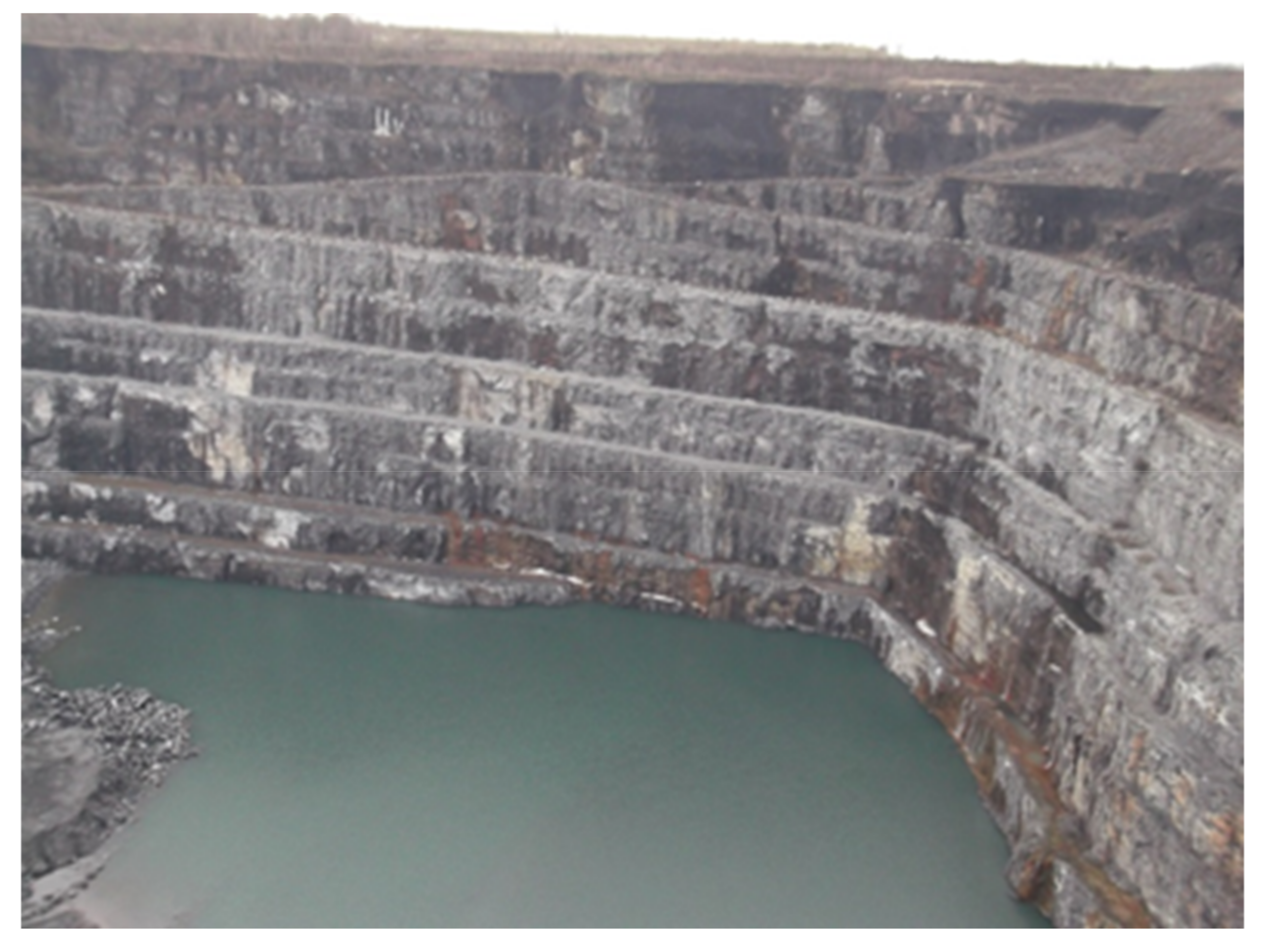
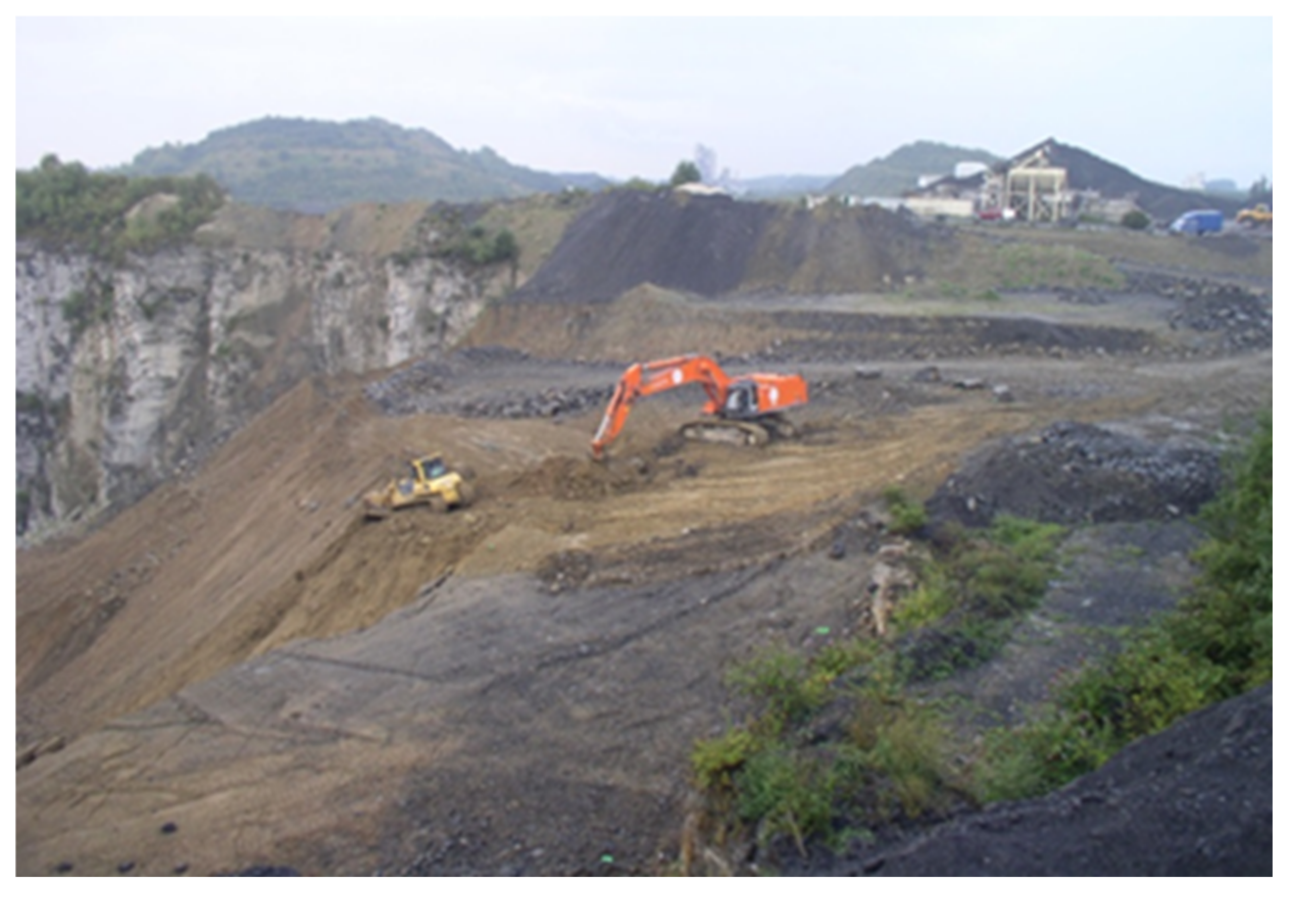
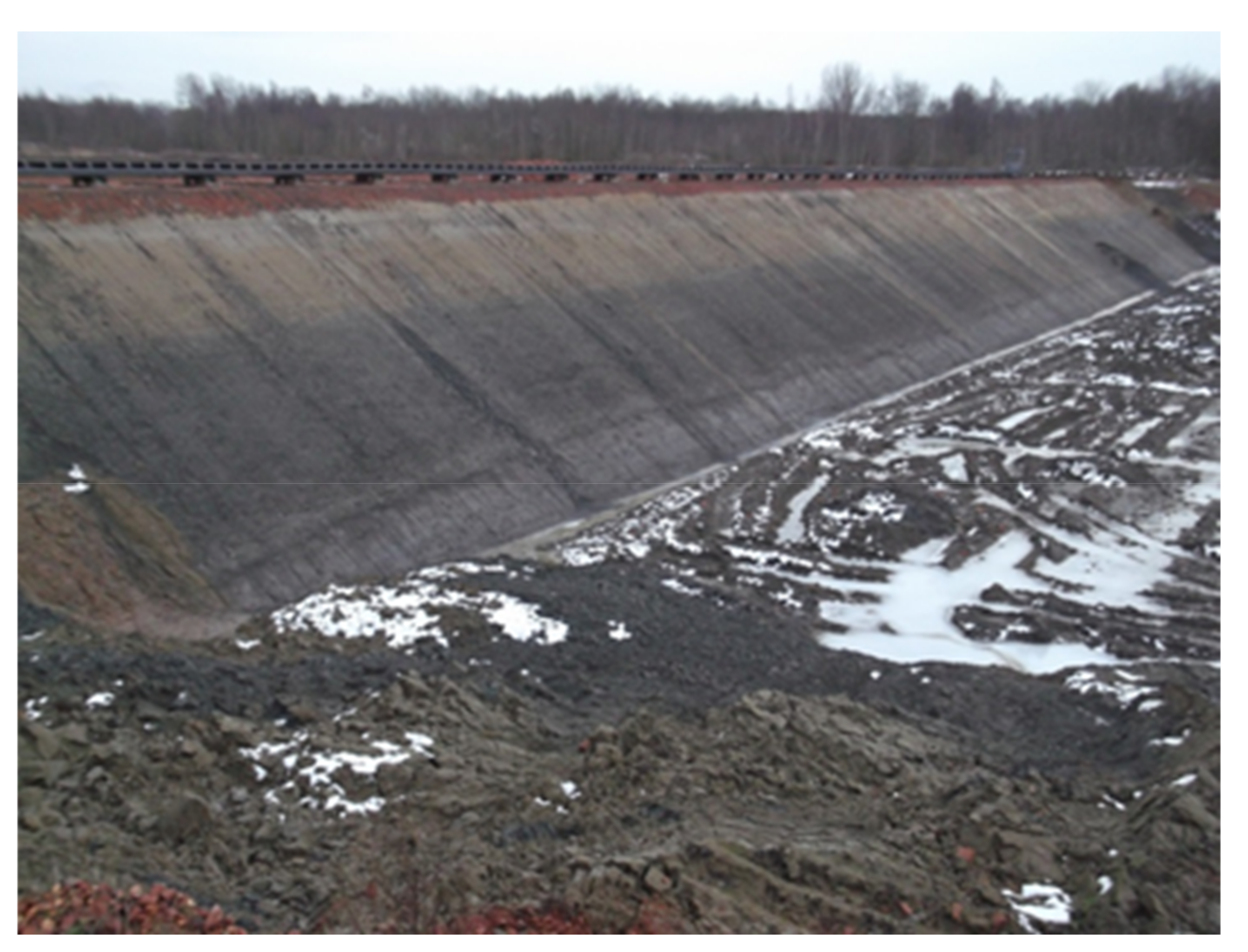
2.1. Quarry Basin Conditions and Problem Definition

The backfilling project aims to gradually fill a pit approximately 1500 m long, 700 m wide, and 240 m deep (absolute elevation of the pit bottom at −205 m ASL) over about 20 years. The filling is carried out by dumping the material coming from the removal of the overburden and barren levels of both a quarry in operation and of a planned new site. The dumping into the basin is expected to be carried out whilst the water level will raise by about 30 m from the pit base level. Due to the intense pumping operations needed for the quarrying activities in the pit, the local ground water table (GWT) at the time of the investigation was located at about 80 m (−45 m ASL) from the ground surface, as shown on the hydrogeological map of the area [5]. It is expected that the water depth in the pit will be maintained at about 160 m in the future, due to pumping requirements for supplying water to the nearby plant. Figure 1 shows a section of the open pit with the lake at an elevation of about −190 m ASL. (i.e., a water depth of 15 m in the pit).

The accumulation of coarse material in the basin and the increase in the water level will lead to an increase in the amount of fine material dispersed in water, which will affect both the turbidity values and the sulphate content in the water. Therefore, the prediction of the potential impact of the turbidity and release of sulphate ions in the pit is crucial in order to plan the dumping and the backfilling activities.

The expected average value of solid flow entering the basin is about 1000 m³/h, consisting of a mix of clay and black silty sand in equal proportion. Minor quantities of other barren materials (such as coarse rock debris) are not supposed to change the boundary conditions. Therefore, the muck flow is significant, although not exceptional [26]. The topic of time rate and planning of disposal within pit lakes has already been discussed in the literature [27].

The quarry basin will be progressively filled by the groundwater flow coming from the pit walls. The overall balance of water must also consider the recirculation of water for plant operations (washing of granulates) as well as the rainfall contribution. The available volume in the exhausted pit is comparable to the volume of overburden to be dumped. However, due to incertitude on the actual consolidation of the mineral waste in the water (i.e., its final volume after dumping) and to the long-term strategy of reclamation of the site, still under evaluation by local authorities, the final rate of filling of the pit is unknown, although it is expected that a lake will be left in place.

The recharge due to the groundwater flow is not constant, but a differential between inflow and pumping values comprising 9 Mm³/year of water can be assumed in order to follow a progressive raising of the water level in the basin. The pumped water should be returned to the superficial hydrological network by respecting the limit values of turbidity and concentration of sulphate ions. The reference values are 45 mg/L for the turbidity (after a water treatment process) and 250 mg/L as far as the concentration of sulphate ions is concerned.

The presence of sulphate ions in the Carboniferous limestone aquifer in the area has been investigated in the literature [28]. The high (and highly variable) presence of sulphate ions was attributed to complex geochemical processes driven by water–rock interaction and ion exchange. The origins of sulphate ions in groundwater were associated with the oxidation of sulphur minerals such as pyrite or marcasite, as well as with the dissolution of evaporites [28].

Background sulphate concentrations between 400 and 450 mg/L were recorded in the pit lake water used for the trial (see Section 3.2), suggesting that a hypothetical sulphate removal plant should ensure at least an abatement of about 200 mg/L, even without considering the effects of the waste burden backfilling. The interest of the research was, therefore, to assess whether the backfilling would have had a significant effect on the water treatment requirements and plant design.

The complexities deriving from the backfilling of solid materials at a high rate, possibly from several dumping points [25], as well as from the dynamic effects of groundwater inlet and pumping activities on the water level and flow in the pit, outweighed the potential of simplified analyses based on existing knowledge from designing and operating settling ponds. The investigation, therefore, focused on the design and operation of a large trial pit simulating the backfilling conditions.

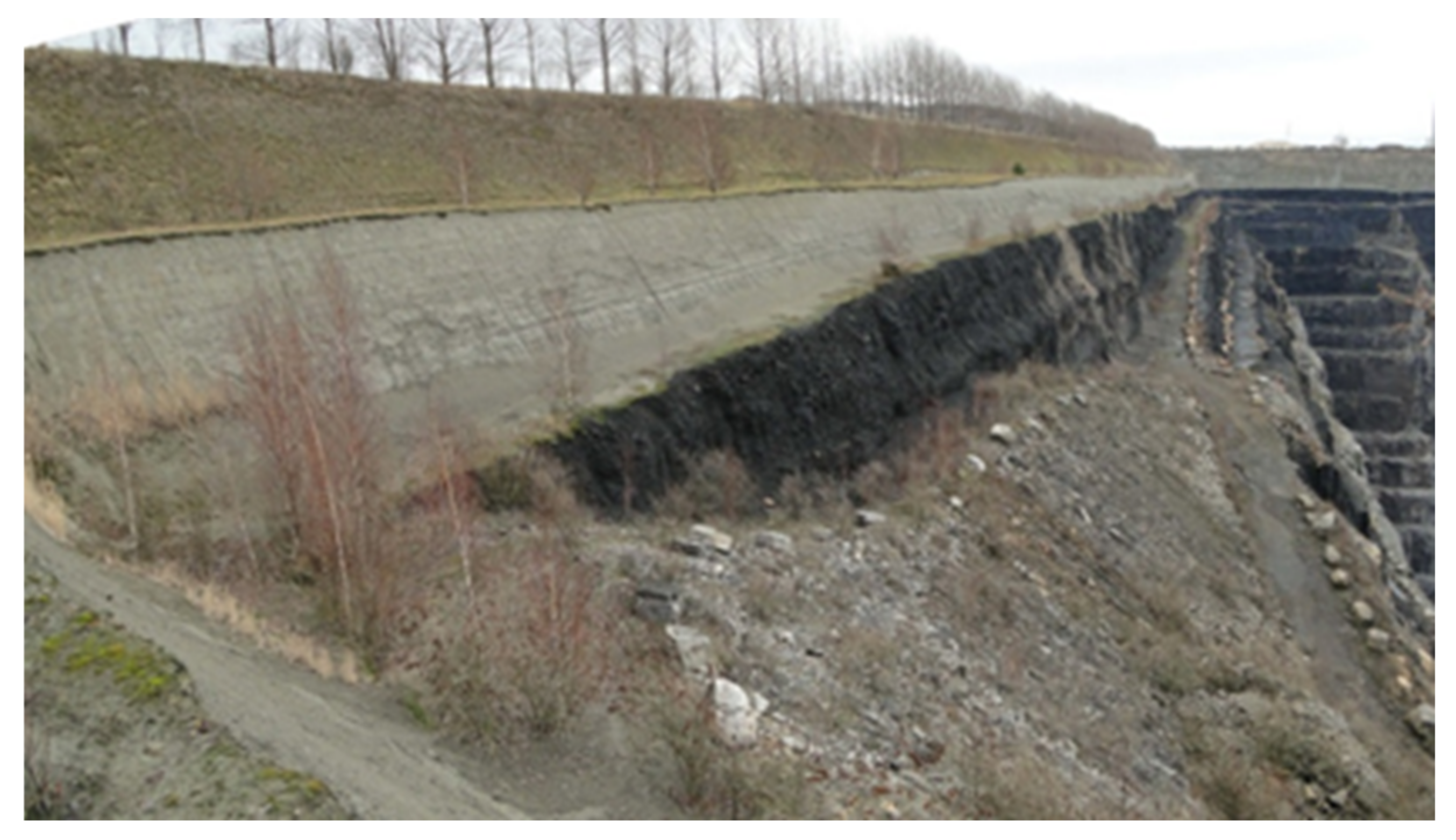
2.2. Geotechnical Properties of the Dumped Material

The geological sequence of the quarry site was characterised by a relevant regional limestone formation in central Europe, horizontally stratified, with a repetition and alternation of strata 4 m to 20 m thick. Further details on the geological cross section of the limestone deposit can be found in the literature [25]. The rock mass consisted of different types of carbonatic compositions and quicklime grades, and it was covered by a thick overburden (up to 30 m) made of two to three different types of soil, depending on the location in the region. Both the newly planned quarry (from which the overburden was coming) and the existing open pit to be backfilled belonged to the same geological formation and to the same hydrogeological domain.

The overburden materials were classified in terms of geotechnical parameters as well as according to the possible alternative disposal methods, i.e., as sludge through pipelines, as lumps through conveyor belts, as bulk by dumping with trucks (see Figure 2).

Further to the cover soil, consisting of silty sand and generally recovered for agricultural purposes, the main soil types are referred to:

• Grey clay, generally of high plasticity (CH) (see Figure 3).
• Brown clay, of intermediate to high plasticity (CH).
• Dark silty sand of low plasticity (SC).

Other materials included detritus barren rocks or dark limestone top layers (see Figure 4). The geotechnical and physical parameters measured assessed for the three soil types are summarised in

Table 1. Summary of geotechnical and physical characterisation of burden soils.

Soil Type	Particle Density (g/cm3)	Bulk Density (g/cm3)	Natural Water Content (%)	Grain Size (%)			Consistency Indices				Classification
				<2 μm	<20 μm	<75 μm	LL 1 (%)	PL 2 (%)	PI 3 (%)	CI 4 (%)	AASTHO 5	USCS 6
Grey clay	2.66	1.90–1.93	34.4	45–68	87	99	95.5	30.6	64.9	0.94	A-7-5 A-7-6	CH
Brown clay	2.66	1.90–1.93	32.3	38–51	62	99	73.6	28.3	50.3	0.82	A-7-6	CH
Dark sand	2.65	1.87–1.92	17.1	22	28	46	41.5	23.0	18.0	1.36	A-7-5	SC

¹ Liquid limit; ² Plastic limit; ³ Plasticity index; ⁴ Consistency index; ⁵ American Association of State Highway and Transportation Officials; ⁶ Unified Soil Classification System.

.

Full details for the geotechnical characterisation of the materials following laboratory and in situ tests were provided by Oggeri et al. [25].

2.3. Pilot Basin Test

2.3.1. Basin and Operation Design

A real-scale experiment for the assessment of the effect of material dumping in water was designed as follows:

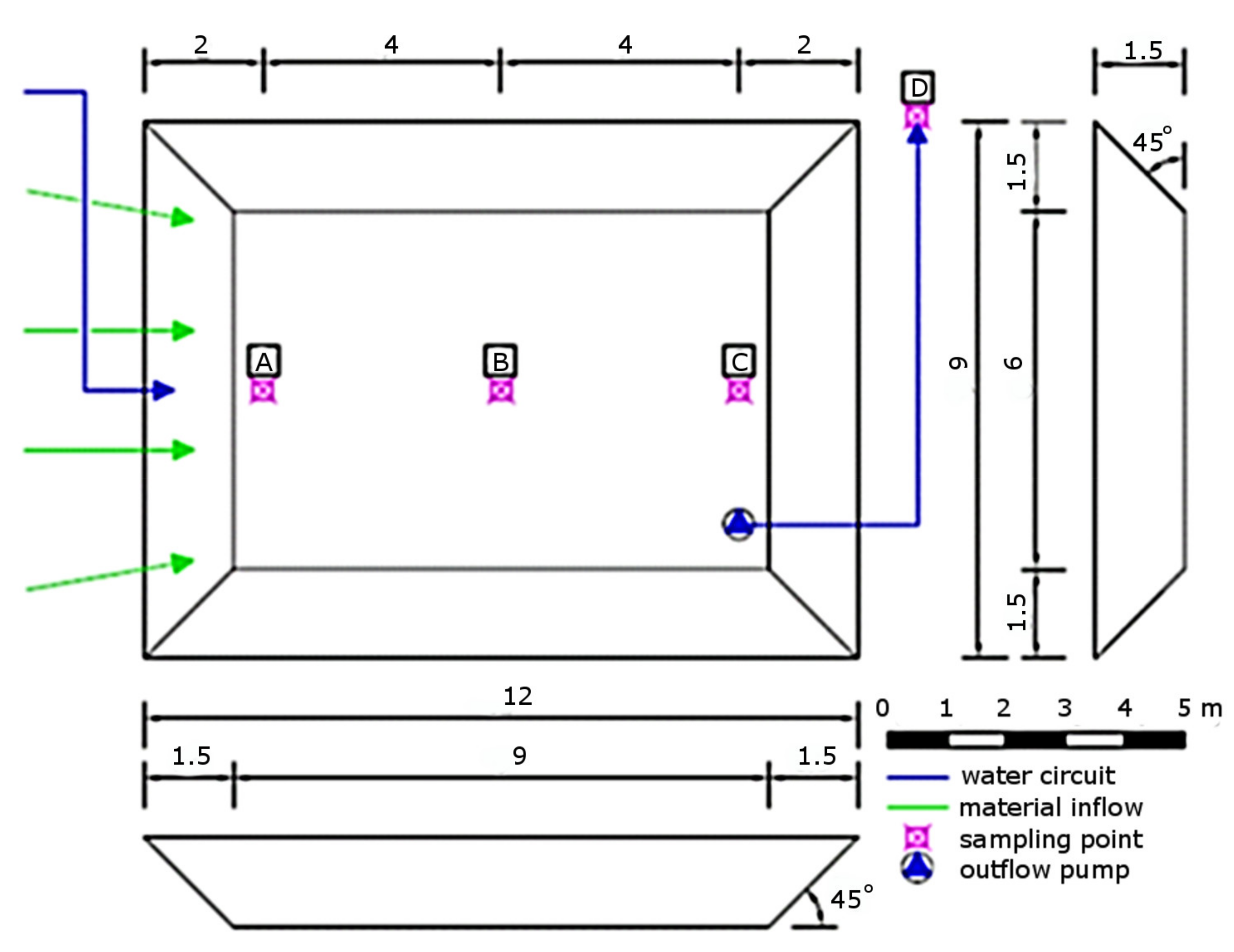
• A pond (basin) of about 100 m³ and two metre depth was excavated. A HDPE liner prevented seepage from the pond to the subsoil.
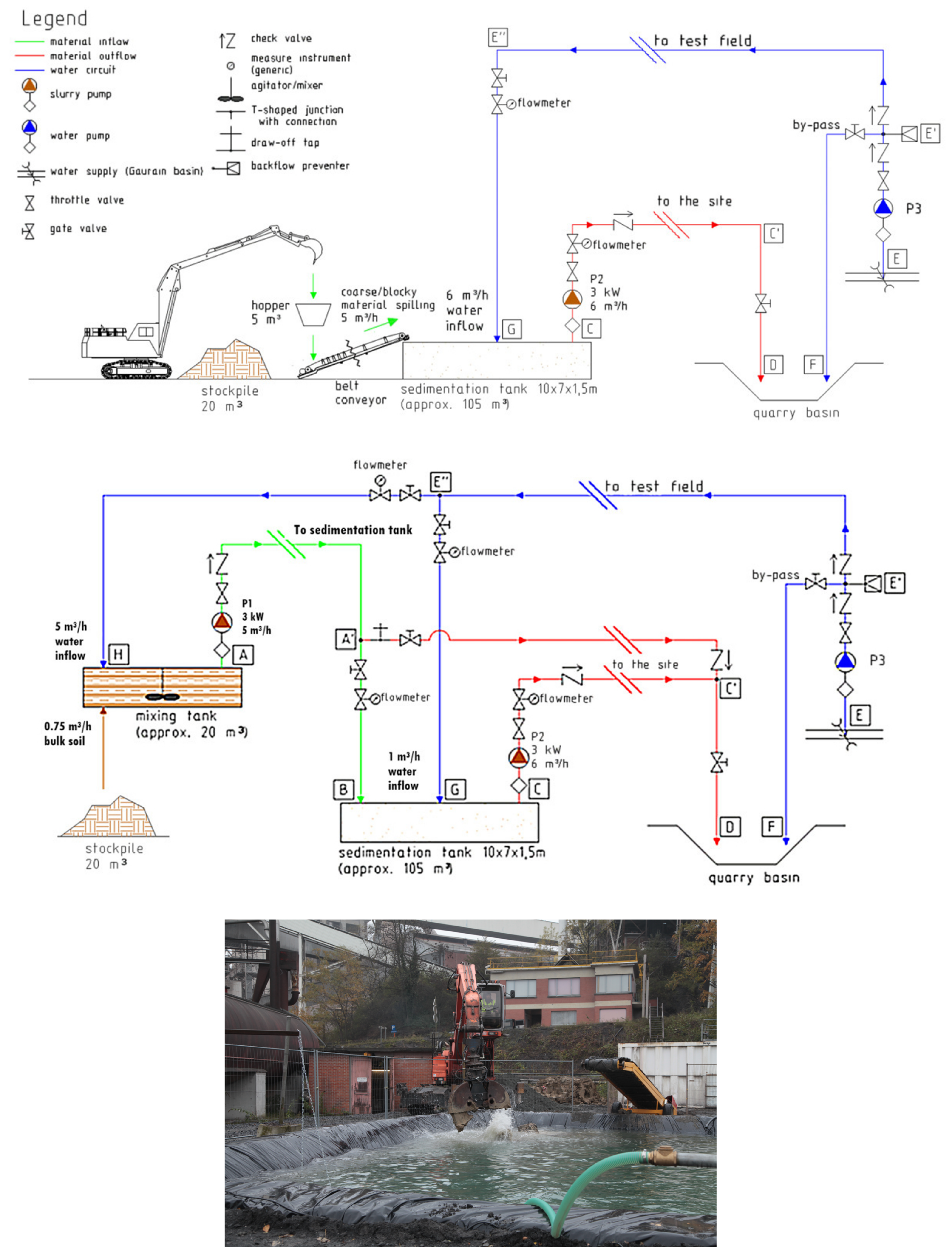
• A metallic vessel was adopted for the initial storage and mixing of the solid geomaterials. The mixing was carried out with two vertical shaft mixers and a slurry pump. An additional and more powerful horizontal shaft mixer was added to the system after some preliminary tests suggested that the two smaller mixers were not meeting the blending requirements.
• A hydraulic alimentation circuit to feed the basin and the vessel with water pumped from the quarry lake. The inflow hydraulic circuit for feeding the main basin from the mixing vessel, equipped with a closure, regulating valves, and flowmeters.
• A hydraulic outflow circuit for pumping out the water from the basin, equipped with a closure, regulating valves, and flowmeters.

The scheme of the pilot basin and the material feeding operation schemes are shown in Figure 5 and Figure 6, respectively, whilst the main geometrical parameters of the pilot basin are provided in

Table 2. Main geometrical parameters of the pilot test basin.

Parameter	Dimension	Unit
Average length	70.0	m
Average width	7.0	m
Water depth	1.2	m
Flow section	8.4	m2
Volume	105	m3

.

2.3.2. Test Procedure

The experiment involved the progressive backfilling of the test basin with coarse material by using mechanical means (belt conveyor and bucket excavator). The test started with a volume of about 80 m³ of water in the basin. During the first day of test, a total amount of about 16 m³ of solid material was added by means of a belt conveyor. The test was carried out in two main parts:

• Steady state conditions (days 1–6), focusing on the behaviour of the turbidity and release of chemical substances after the backfilling of the basin with about 16 m³ of material (sand and clay in the same proportions) at a constant basin water volume (without any water inflow and outflow).
• Dynamic conditions (days 7–14), with an intermittent water inflow and outflow to simulate the effect of potential lixiviation and transport due to the water flow into the basin. Intermittent soil back-filling operations were carried out to simulate the effect of material falling in lumps on turbidity and release of chemicals.

From day 7 to day 10, new solid material was added in the basin with an average rate of about 10 m³/day. The water inflow and outflow were adjusted in order to gradually increase the lixiviation effect of the solid as well as the degree of diffusion and dispersion of substances into the basin. During the last day of backfilling (day 10), no water inflow was allowed. The outflow started at 8.50 a.m., with a short break for maintenance of the devices between 9.30 a.m. and 10.00 a.m. The pumping system discharged a total volume of about 14.4 m³ out from the basin to balance the inflow of new solid material. A total volume of about 55 m³ of solid material was added in total during different phases into the basin.

During the last two days (day 13 and 14), the activities were focused on checking the response of the system without any addition of solid material by controlling a reduced inflow and outflow rate. The water volume into the basin was gradually reduced from 80 m³ up to about 25–27 m³ at the end of the experiment.

During the experiment, a constant wind (1–2 m/s) was detected, mainly oriented from west toward east, i.e., on the opposite direction of the inflow–outflow direction of material flows. The perturbation on the basin due to the wind was of the same order of magnitude of the induced flow rate, as the surface velocity was found to be reduced.

Table 3. Water inflow and outflow and volume of the backfilled solid material.

Day	Hour (h:min)	Time (h)	Water						Soil Material Filling				Volume Balance Analysis
			Inflow	(m3)	(l/s)	Outflow	(m3)	(l/s)	Sand (m3)	Clay (m3)	Total (m3)	Cumul. (m3)	Water (m3)	Basin (m3)
1	9:45	0.0	Sampling
	10:20	0.6		0.0	0.0		0.0	0.0	8.0	8.0	16.0	16.0	80.0	96.0
7	9:15	143.5	Start	0.0	0.65	Start	0.0	0.79	5.0	5.0	10.0	26.0	75.3	101.3
	17:45	152.0	Stop	20.5
	18:05	152.3				Stop	25.2
8	9:15	167.5	Start	0.0	0.46	Start	0.0	0.88	5.0	5.0	10.0	36.0	61.2	97.2
	16:00	174.3	Stop	11.5
	17:00	175.5				Stop	25.2
9	9:00	191.3				Start	0.0	0.39	5.0	5.0	10.0	46.0	47.5	93.5
	18:50	201.1				Stop	13.7
10	9:00	215.3				Start	0.0	0.48	5.0	5.0	10.0	56.0	33.1	89.1
	17:20	223.6				Stop	14.4
13	10:15	288.5	Start	0.0	0.56				0.0	0.0	0.0	56.0	33.1	89.1
	10:20	288.6				Start	0.0	0.51
	14:30	292.8	Stop	8.5
	15.00	293.3				Stop	8.5
14	9:10	311.4	Start	0.0	0.3	Start	0.0	0.72	0.0	0.0	0.0	56.0	26.2	82.2
	13:45	316.0	Stop	4.9		Stop	11.8

summarises the data on soil filling, inflow and outflow water, and volume balance analysis, with their effective reference times. The table is organised in the following columns: day of test, hour of sampling, effective time from a reference time with initial value equal to zero, inflow and outflow water that generated flow conditions, soil material filling expressed as clay, sand, total and cumulative, and cumulative volumes (water volume and basin volume).

2.3.3. Water Monitoring and Sampling

The location of the points for the monitoring of physical parameters and for water sampling are shown in Figure 5, labelled A, B, C and D. Sampling points A, B, and C were aligned along the centre line of the basin, close to the inflow position (A), in the middle of the basin (B), and at the end of the basin (C), respectively. Station D refers to the sampling at the outflow of the pipeline.

The water was sampled on the upper layer (depth of about 0.3 m) using a water sampler with a volume of 0.5 L.

The chemical–physical monitoring on-site involved the measurement of water temperature (T), electrical specific conductivity (SpC), pH, dissolved oxygen (DO% and DO), and oxidation-reduction potential (ORP) through a water quality multi-probe device (MiniSonde 4a, manufactured by Hydro Lab).

Water was extracted from the water sampler and injected into sterile bottles using a syringe equipped with a filter with a cut-off 0.45 μm in order to eliminate the particulates that could potentially interact with the liquid, as per the methodology described in the UNI 10802 and in agreement with the EC directive EN 12457/2.

The concentration of solid particles (C_S) and contents of sulphate ions (SO₄²⁻) were obtained from turbidity calibration and chemical laboratory tests, respectively. In total, 85 water tests were performed, and 54 samples for chemical analyses were collected in total.

Nephelometric Turbidity Unit (NTU) was adopted for assessing the turbidity. As the NTU scale is a qualitative index, a calibration exercise was required for correlating NTU with solid particle concentrations in water.

The calibration procedure was carried out by stirring, in a constant water volume (2 l container), an increasing mass of sand and clay from the site (blended in the same quantity; therefore, replicating on-site test soil dumping), thus increasing the solid particle concentration and measuring turbidity values at each step. An Aqualytic infrared turbidity meter AL250T-IR was used. The unit measured the scattered light at an angle of 90°, according to the standard EN ISO 27 027, in a range 0.01 to 1100 NTU. The concentration of solid particles was prepared in the range of about 10 to 800 mg/L. The results of the calibration led to a linear relationship between the turbidity (NTU scale) and the solid content (C_S, mg/L). The obtained empirical relationship was Cs ≅ 5 NTU. However, as the relationship was valid only for the specific turbidity testing ranges and for the two tested soils, the details on its determination were not reported here as not deemed relevant.

The determination of sulphate ion concentration was carried out using ion chromatography technique.

2.4. Analytical Models for Sedimentation and Sulphate Release Prediction

2.4.1. Sedimentation Model of Hazen–Stokes

The model was developed for computing the solid dispersed concentration and analysing the sedimentation process of the coarse material with Stokes’ sedimentation law and Hazen’s theory. It should be underlined that the backfilling was not as regular as requested by a proper modality to supply the material inside the basin. Nevertheless, the analytical approach fitted the physical behaviour, and the computed concentration values were found to be in the same order of magnitude of the measured data.

Two main scenarios were taken into account:

• The addition of soil and estimation of the sedimentation time of particles with a specified grain size.
• The mobilisation of the solid particles and chemical substances released by the soil by applying a controlled water flow in the basin.

For both scenarios, the sedimentation velocity was calculated at 3 m and 6 m, far from the soil discharge point in the basin, then the correspondent theoretical critical particle diameter was selected, as well the time for sedimentation in the first 20 cm below the water level.

The horizontal average velocity was calculated in order to receive a representative motion inside the basin.

Considering the properties of the two natural soils and their grain size distributions, an estimation of the solid particle content, suspended in water, was performed according to the following formula:

C_S = Q · h · P_gs · ρ_s · 10⁶ · 1/V · μ_lib · μ_lump

(1)

where:

• C_S is the concentration of solid particles in mg/L.
• Q is the flow rate in m³/h.
• h is the effective dumping period in hours.
• P_gs the percentage of fine material from the cumulative grain size distribution (from 20 to 25% for the dark silty sand).
• ρ_s is the grain density in kg/m³.
• V the basin volume in litres (it was observed that the whole volume of the basin was involved by the wave motion during the solid filling).
• μ_lib is the degree of liberation of fine grains due to the cohesive properties of the silt, assumed to be about the 50% of the available soil.
• μ_lump is the degree of soil that is released directly from the lumps and that remains in suspension after the sedimentation of the majority of coarse grains in the measuring period. According to preliminary sedimentation tests in laboratory, this coefficient was estimated in the range 0.01 to 0.05.

2.4.2. Sulphate Mass Balance Analytical Calculation

The silty/clayey fraction of the material introduced in the test basin was considered the main responsible for the fine particle dispersion and, consequently, for the release of sulphate ions in water.

The sulphate concentration in the pilot test could be assessed by considering the water inflow and outflow rates, the volume of solid material, and the water volume within the basin. The mass balance was critical to estimate the potential lixiviation effect of the solid material in terms of mass of sulphate released per unit mass of solid (parameter M_sul).

These data could be used both to estimate the dispersion rate, i.e., the capability of the material to release sulphate ions, as well as to predict the sulphate release at the scale of the quarry basin.

The mass of sulphate ions in the pond at the end of each day (M₁) could be calculated as:

M₁ = M₀ + M_w + M_lix − M_out

(2)

where:

• M₁ is the mass of sulphate ions in the pond at the end of each day.
• M₀ is the mass of sulphate ions at the beginning of each day.
• M_w is the mass of sulphate ions brought into the pond by the feeding water (background concentration).
• M_lix is the mass of sulphate ions lixiviated from the solid material.
• M_out is the mass of sulphate ions extracted with the water pumped out.

As the masses of sulphate ions in water could be calculated as the concentrations of sulphate (in mg/L) multiplied by the relevant volumes, and Equation (2) could be rewritten as:

C₁ V₁ = C₀ V₀ + C_w,i V_w,i + M_lix − C_out V_out

(3)

where:

• C₁ is the concentration of sulphate ions in the pond at the end of each day.
• V₁ is the volume of water in the pond at the end of each day.
• C₀ is the concentration of sulphate ions in the pond at the beginning of each day.
• V₁ is the volume of water in the pond at the beginning of each day.
• C_w,i is the background concentration of sulphate ions in the feeding water.
• V_w,i is the volume of water fed in the pond.
• M_lix is the mass of sulphate ions lixiviated from the solid material.
• C_out is the concentration of sulphate ions in the water pumped out.
• V_out is the volume of water pumped out of the pond.

Under the simplified hypothesis that the sulphate concentration in the water pumped out was equal to the average daily concentration:

C_out = (C₀ + C₁)/2

(4)

Equation (3) could be rewritten as:

C₁ (V₁ + V_out/2) = C₀ (V₀ − V_out/2) + C_w,i V_w,i + M_lix

(5)

Lixiviation (or solid–liquid extraction) is the process of separation of one or more soluble components from a solid mass by means of a solvent, being water in this case. The goal was to estimate the mass of sulphate ions (parameter M_lix) obtained from the lixiviation of the coarse material in test basin, under the action of a flow field.

The daily mass of sulphate (M_lix) was, therefore, obtained by rewriting Equation (5) as:

M_lix = C₁ (V₁ + V_out/2) − C₀(V₀ − V_out/2) − C_w,iV_w,i

(6)

By focusing on the sulphate concentrations sampled at point C and point D (only for the flow case), the values of M_lix were obtained using Equation (6). This procedure was followed for two background concentration scenarios, i.e., an initial sulphate concentration (C_w,i) equal to 400 mg/L in the first case and 450 mg/L in the second case, using inflow and outflow volumes provided in Table 3.

The dispersion rate, i.e., the mass of sulphate ions with respect to the amount of the soil dumped in the basin (M_sul, expressed in milligrams of sulphate ions per kilograms of solid mass), corresponded to the ratio between the sum of the sulphate mass derived from the solid lixiviation and the cumulative solid mass introduced in the basin:

M_sul = (∑(M_lix)/K)/(∑ M_sol)

(7)

where:

• M_lix is the mass of sulphate ions.
• K is the clay–sand repartition coefficient, assumed equal to 0.5.
• M_sol is the quantity of clay–sand introduced in the test basin.

The introduction of the parameter K = 0.5 implicitly assumed that only half of the mass of the soil would contribute to the release of sulphate. This hypothesis was made according to the results from column sedimentation tests on the same soils described by Oggeri et al. [25]. The outcomes from the sedimentation tests suggested that the clay fraction, due to its sticky behaviour, was unlikely to disperse fine particles in the water, as the relatively high cohesion and marked plasticity resulted in the formation of clumps and clods. This behaviour might prevent the fine fraction from clay to pass in suspension, thus reducing the available exposed surface of the soil particle for a significant sulphate release. For this reason, it was assumed that the sand fraction was the main responsible for the sulphate release, thus neglecting the mass of clay in the model.

3. Results

The water quality monitoring (on-site) allowed us to record turbidity values and sulphate concentrations. Specific conductivity and water temperature were also measured for control purposes. The specific water conductivity was a good indicator of the relative changes in dissolved ions (electrical charge) in water. It was observed that electrical conductivity showed stable values with small oscillations around the central value of 1000 μS/cm.

3.1. Turbidity Value Results

The measure of turbidity was found to be very sensitive to the perturbation induced by the backfilling activity. A background value of about 9 NTU (approx. 46 mg/L) was recorded just before the backfilling, followed by a sudden and sharp increase, up to 80–90 NTU, during the backfilling activity, and then by a sharp decrease to values of about 35 NTU at the end of the first day of testing.

The turbidity level was similar to the background values after 20–22 h from the backfilling, and the background level was reached after 28 h. In total, 3 days after the perturbation, the turbidity was found to be 30% lower than the background values. This behaviour may have been due to the turbulence created during the water feeding (only one day before the test) along with the presence of some particulate and sediments in the basin.

During the second day of soil backfilling (day 7), a new sharp increase in the turbidity was observed, recording values up to 85–90 NTU in the basin and 125–130 NTU at the outflow station (D).

A few hours after the backfilling, the turbidity went down to values of about 33–37 NTU in the basin and 42 NTU at the outflow point. A similar behaviour was observed during the subsequent days of solid backfilling. On day 8, a peak of 180–190 NTU at the outflow point was measured, while values within the basin ranged from 85 to 102 NTU.

During the last day of solid backfilling, values higher than 100 NTU, in the ranges of 70–120 NTU after few hours and about 50–70 NTU at the end of the day, were recorded. Towards the end of the test, values in the range of 6–15 NTU were measured both in the basin and at the outflow station.

The conversion of turbidity from NTU to concentrations in mg/L led to peak values of the suspended solids to be estimated in the order of 800–1200 mg/L. These peak values were obtained during the backfilling of solid material. The values of suspended solids’ concentrations returned to background values after a few hours of the water’s flow in steady-state condition, with a flow velocity of about 0.5 m/h.

The trend in the filling, inflow, and outflow of the water volume and the values of the suspended solids’ concentrations at the sampling points B and C are shown in Figure 7. A satisfactory correspondence between the values of solid concentrations and the activity of soil filling can be observed.

3.2. Sulphate Ions Concentration

Two series of water measurements were carried out at points B and C before the backfilling was started in order to evaluate the background values of the sulphate concentration of the feeding water. The results of these two samples indicated moderate-to-high values of electrical conductivity: about 1000 μS/cm (the electrical conductivity of drinking water is typically in the range 100 to 700 μS/cm [29]) and a sulphate ions content SO₄⁻ of about 450 mg/L. It was to be observed that the background concentration of the sulphate ions in the water played a significant role in the final sulphate mass to be considered for designing suitable water treatment plants (needed for any restitution of the water to the surface network, for which the concentration limit is 250 mg/L). A certain degree of incertitude was implicit in the assessment of a suitable value of the background concentration, as:

(a)

The water used for the trial was pumped from the exhaust pit. Due to its significant dimensions, historical measurements of the sulphate concentration showed marked differences when water was sampled at different points of the pit.

(b)

The measurement of sulphate content could be affected by an error that is usually in the range 5–10%.

For the above-mentioned reasons, it was decided to perform a sensitivity analysis of the model using a value representative of the sulphate concentration prior to any backfilling (i.e., 450 mg/L) and a value reduced by about 10% (i.e., 400 mg/L). Due to the possible errors in the analytical determination of sulphate or the representativeness of samples, the precision of rounded values (400 and 450 mg/L) was considered suitable.

A slight increase in the sulphate concentration during the first day of the backfilling was registered, with a peak of 480 mg/L.

At the end of the first phase of the test (day 1 to 6, steady condition, i.e., without water flow), the values of sulphate ions returned to the background values. The concentration raised up to about 500 mg/L during the second week (days 7 to 10) when the addition of new solid material led to an increase in the total amount of the sulphate ions.

During the third stage of the test (day 13 and 14), with constant water inflow and outflow and without any further addition of solid material, the values remained more or less constant at around 500 mg/L.

The values of the concentration of sulphate ions for the samples collected during the test at the sampling points A, B, C, D are summarised in

Table 4. Observed sulphate ions concentration at the different monitoring stations.

Day	Hour	Sampling Point				Note
		A	B	C	D
	(h:min)	(mg/L)	(mg/L)	(mg/L)	(mg/L)
1	9:00	-	441	448	-	Background value before filling
	11:40	453	470	465	-	Backfilling
	17:05	-	482	481	-	Null water inflow–outflow
2	15:40	432	440	430	-	Null water inflow–outflow
3	8:40	471	454	443	-	Null water inflow–outflow
4	13:40	434	442	442	-	Null water inflow–outflow
7	9:00	423	430	432	-	In/out flow active backfilling
	17:45	440	458	462	455	In/out flow active backfilling
8	8:25	424	453	459	-	In/out flow active backfilling
	17:00	473	482	459	464	In/out flow active backfilling
9	7:45	470	484	491	-	In/out flow active backfilling
10	8:50	-	-	475	-	In/out flow active backfilling
	13:30	501	-	474	483	In/out flow active backfilling
	17:15	-	-	-	497	In/out flow active backfilling
13	10:35	499	496	502	505	In/out flow active
	14:45	493	485	501	499	In/out flow active
14	8:15	501	503	503	507	In/out flow active
	13:40	506	501	501	505	In/out flow active

. The two columns, hours, and notes give information about the activities of the addition of coarse material or about the pumping performed before samples were collected.

The interpretation of the results and the description of the concentration of sulphate ions trends were not straightforward, as the physical phenomenon was influenced by dynamic processes of water pumping, fresh soil dumping, and release and possible re-absorption of sulphate ions by the soil. The large-scale trial conditions did not allow us to investigate the sulphate release/absorption dynamics in detail, but they did allow us to appreciate the evolution of the water quality at a whole basin system scale. Data for sampling stations B and C were plotted against the material input/output (see Figure 8). From a qualitative perspective, it could be observed that the background value of 450 mg/L was maintained in the first seven days (static conditions), after an initial peak when the soil was added in the pond. The addition of soil and/or water pumping (i.e., during the dynamic stage of the test) perturbed the sulphate concentration values, with a sharp increase of about 50 mg/L in days 8 to 9. After that, two scenarios could be hypothesised:

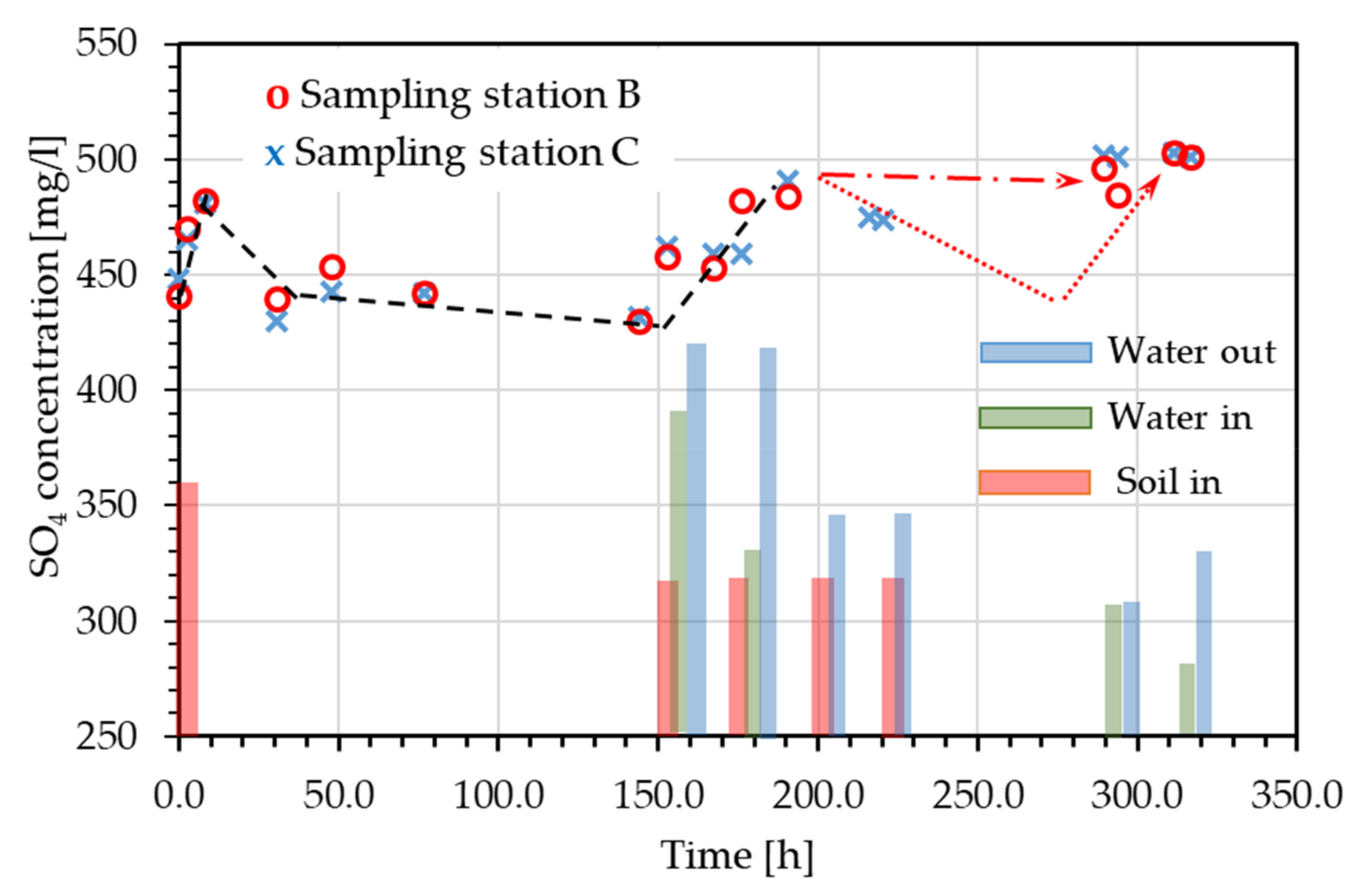
• The sulphate concentration remained more or less constant (or increased slightly), irrespective of the dynamics in the pond (dash dot arrow in Figure 8). The release of sulphate from the soil took place mainly at the early contact of soil with water, after which the effects of water pumping, the variation in the soil/water ratio in the pond, the sedimentation of the soil, and the possible mineral reabsorption of SO₄ broadly maintained the sulphate concentration at the same level.
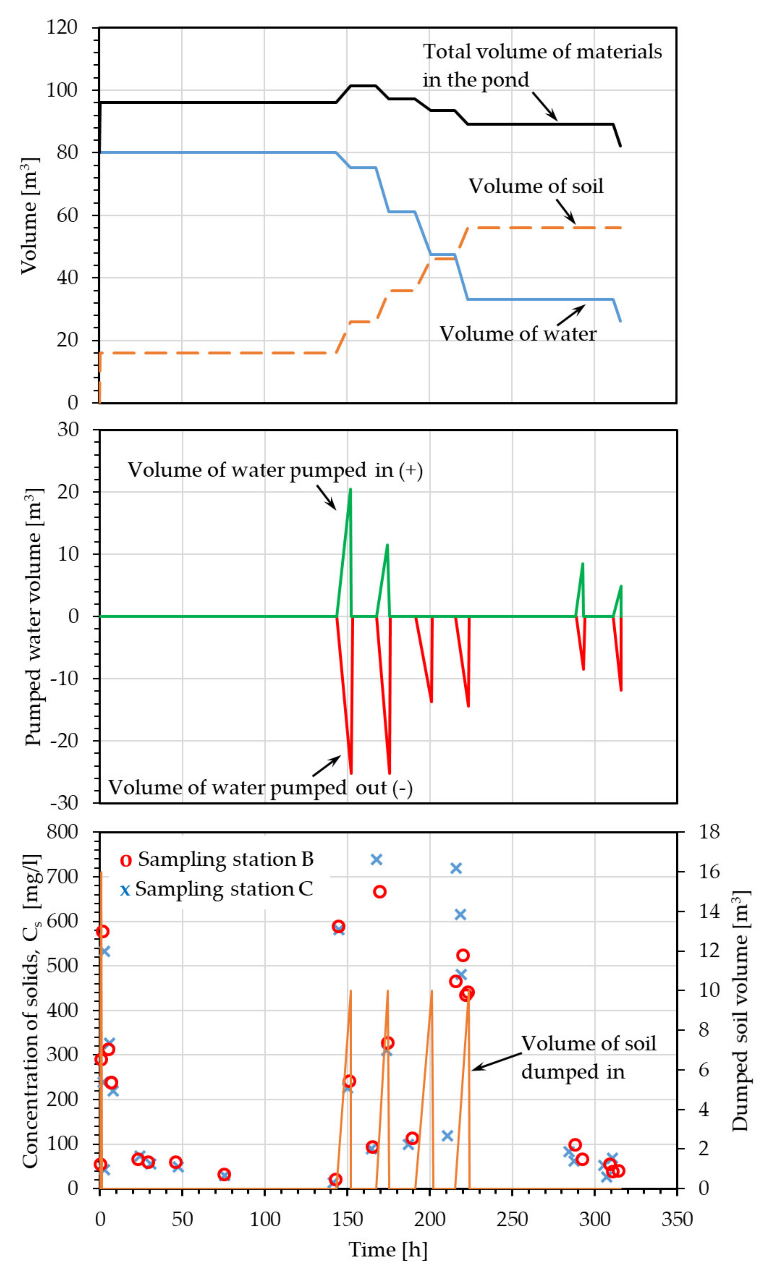
• The sulphate release (and thus concentration) was mainly affected by the turbulence in the pond: the soil dumping and water pumping activities increased the turbulence of the water flow, therefore, increasing the fraction of solid particles in suspension (as observed from the results on concentration of solids, see Figure 7). Under these conditions, the contact between water and particles was fostered by a larger specific surface, and the sulphate release was increased. This hypothesis should acknowledge that the sulphate ions were reabsorbed by the soil under static conditions of water flow (i.e., sulphate concentration decreases, dotted arrow in Figure 8), whereas these were released again by turbulent flow due to water pumping (at 300–320 h).

The obtained results did not allow us to reach a unique option for the most appropriate scenario, depending on the dynamic evolution of physical–chemical processes, thus providing a reliable basis to be used to inform and guide further research.

3.3. Theoretical Assessment of Suspended Soil Particles

The theoretical assessment of the suspended solids’ particles in water was carried out following the approach described in Section 2.4.1.

Table 5. Summary of sedimentation velocity and deposition time for several critical diameters.

Flow Rate Q (m3/h)	Parameter	Position		Horizontal Flow Velocity
		3 m, Point B	6 m, Point C	m/s	m/h
2.5	Sedimentation velocity	3 × 10−5 m/s	1.5 × 10−5 m/s	0.0001	0.36
	Sedimentation time	6600 s	13,300 s
	Critical diameter	0.006 mm	0.004 mm
8	Sedimentation velocity	9.9 × 10−5 m/s	4.9 × 10−5 m/s	n.a.	n.a.
	Sedimentation time	2000 s	4000 s
	Critical diameter	0.012 mm	0.007 mm

shows the range of theoretical critical diameters that could influence the sedimentation process and summarises the results of the Hazen–Stokes approach on the sedimentation process for several theoretical critical diameters (4, 6, 7, 12 μm). The turbidity was spreading inside the basin following the wave motion and not following the flow velocity. The theoretical relationship (from Stokes’ model) between the sedimentation velocity and particle diameter is shown in Figure 9.

The calculated values were higher than the measured data (see

Table 6. Comparison between calculated and measured C_S.

Flow Rate Q (m3/h)	Point B			Point C
	Time (h)	CS,calculated (mg/L)	CS,measured,max (mg/L)	Time (h)	CS,calculated (mg/L)	CS,measured,max (mg/L)
2.5	1.8	159	95	3.6	127	77
8	0.55	775	587	0.55	620	517

). Nonetheless, these were comparable both as far as the trend and the order of magnitude were concerned. It was to be recalled that the calculated C_S came from Equation (1), while the measured C_S were obtained from NTU (turbidity measurement values) through a calibration exercise.

3.4. Sulphate Ions Concentration

As discussed in Section 2.4.2, Equation (6) was used to obtain an estimation of the mass of the sulphate ions released by the solid material dumped in the pond (M_lix). The sulphate concentration values collected at point C and at point D from day 7 to day 14, shown in Table 4, along with the pumping volume data from Table 3 were used under two sulphate inflow concentration scenarios, i.e., 400 mg/L and 450 mg/L.

Both data series collected at point C and D (outflow) showed gaps: some appeared to have been sampled only at the beginning of the day, while others did not seem to have been collected (due to episodic critical weather). Results are shown in

Table 7. Released mass of sulphate ions (M_lix) with C_w,i = 400 mg/L and 450 mg/L. Water volumes and concentrations data from Table 3 and Table 4. Data observed at sampling station C.

Day	Cw,i (mg/L)	C0 (mg/L)	C1 (mg/L)	V0 (m3)	Vw,i (m3)	Vout (m3)	V1 (m3)	Mlix (g)	Mlix (kg)
Day 1	400	-	-	-	-	-	-	-	-
Day 7	400	432	462	80	20.5	25.2	75.3	3293.0	3.2930
Day 8	400	459	459	75.3	11.1	25.2	61.2	654.9	0.6549
Day 9	400	-	-	61.2	0	13.7	47.5	-	-
Day 10	400	475	497	47.5	0	14.4	33.1	886.6	0.8866
Day 13	400	502	501	33.1	8.5	8.5	33.1	829.7	0.8297
Day 14	400	503	501	33.1	4.9	11.8	26.2	440.5	0.4405
Day 1	450	-	-	-	-	-	-	-	-
Day 7	450	432	462	80	20.5	25.2	75.3	2268.0	2.2680
Day 8	450	459	459	75.3	11.1	25.2	61.2	99.9	0.0999
Day 9	450	-	-	61.2	0	13.7	47.5	-	-
Day 10	450	475	497	47.5	0	14.4	33.1	886.6	0.8866
Day 13	450	502	501	33.1	8.5	8.5	33.1	404.7	0.4047
Day 14	450	503	501	33.1	4.9	11.8	26.2	195.5	0.1955

and

Table 8. Released mass of sulphate ions (M_lix) with C_w,i = 400 mg/L and 450 mg/L. Water volumes and concentrations data from Table 3 and Table 4. Data observed at sampling station D.

Day	Cw,i (mg/L)	C0 (mg/L)	C1 (mg/L)	V0 (m3)	Vw,i (m3)	Vout (m3)	V1 (m3)	Mlix (g)	Mlix (kg)
Day 1	400	-	-	-	-	-	-	-	-
Day 7	400	-	455	80	20.5	25.2	75.3	-	-
Day 8	400	-	464	75.3	11.1	25.2	61.2	-	-
Day 9	400	-	-	61.2	0	13.7	47.5	-	-
Day 10	400	483	497	47.5	0	14.4	33.1	564.2	0.5642
Day 13	400	505	499	33.1	8.5	8.5	33.1	668.4	0.6684
Day 14	400	507	505	33.1	4.9	11.8	26.2	460.1	0.4602
Day 1	450	-	-	-	-	-	-	-	-
Day 7	450	-	455	80	20.5	25.2	75.3	-	-
Day 8	450	-	464	75.3	11.1	25.2	61.2	-	-
Day 9	450	-	-	61.2	0	13.7	47.5	-	-
Day 10	450	483	497	47.5	0	14.4	33.1	564.2	0.5642
Day 13	450	505	499	33.1	8.5	8.5	33.1	243.4	0.2434
Day 14	450	507	505	33.1	4.9	11.8	26.2	215.1	0.2151

.

For both sampling stations (C and D), it could be observed that the higher quantity of coarse material introduced during the days in the basin test produced a strong lixiviation, and it determined, therefore, a high value of the released mass of sulphate ions (especially in day 7). Similar considerations could be made for a background concentration of 450 mg/L, i.e., a higher release on the first days compared to the last days.

The parameter M_sul had been calculated only for the data observed at the station C because the dataset from point D was incomplete. Even in this case the simulation was carried out for the two background concentrations (400 mg/L and 450 mg/L) in order to estimate the sensitivity of the results (see

Table 9. Calculation of dispersion rate parameter M_sul for the two scenarios of background sulphate concentration.

Day	Vsoil (m3)	Msoil_cum (kg)	Mlix (Cw,i = 400 mg/L) (kg)	Mlix (Cw,i = 450 mg/L) (kg)
Day 1	16	25,600	-	-
Day 7	10	41,600	3.293	2.268
Day 8	10	57,600	0.6549	0.100
Day 9	10	73,600	-	-
Day 10	10	89,600	0.8866	0.8866
Day 13	0	89,600	0.8297	0.4047
Day 14	0	89,600	0.4405	0.1955
Total		89,600	6.105	3.855
	Msul (mg/kgsoil)		136.2645	86.0413

). The parameter soil volume (V_soil) referred to volume of soil dumped in the basin during the experiment. The bulk density of the dumped soil was estimated on site by measuring the mass of soil in graduated containers. Due to the excavation/handling operations and the consequent bulking of the soil (i.e., increase in volume due to the loss of compaction), the bulk density (used for transforming the volume of soil dumped into the pond into a mass) was assumed to be equal to 1600 kg/m³. Other variables involved were the background concentrations (C_w,i), the cumulative mass of solid (M_{sol_cum}), and the sulphate mass released by lixiviation (M_lix) calculated in Table 7. By inputting the total values of M_{soil_cum} and M_lix in Equation (7), it was possible to calculate the dispersion rate M_sul, expressed in mg of sulphate ions per kg of solid mass.

The results were as follows:

• M_sul = 136.2645 (mg/kg_soil) under the hypothesis of a sulphate background concentration of 400 mg/L.
• M_sul = 86.0413 (mg/kg_soil) under the hypothesis of a sulphate background concentration of 450 mg/L.

The obtained values for M_sul allowed us to carry out an inverse analysis aimed at checking the results from the calculation of mass balance of sulphate ions by lixiviation. This procedure was repeated for the two values of background concentration (400 and 450 mg/L).

The parameter M_sul was assumed as a rate of release of sulphate ions during field testing, obtained considering seven test days (five days in which new coarse material was introduced in the pilot basin, i.e., days 1, 7, 8, 9, 10, and two days in which the release of sulphate ions was monitored, i.e., days 13 and 14).

The released sulphate mass in any day “i” (M_lix,i) could, therefore, be obtained by multiplying the value of M_sul by the mass of dumped soil material and dividing by the number of days in which the coarse material was disposed, or during which there was a release of sulphate ions (seven days), as in Equation (8):

M_lix,i = (M_{sol_cum,i}·M_sul)/7

(8)

The cumulated mass of released sulphate was calculated adding the mass released on each day “i”:

M_lix = ∑ (M_lix,i)

(9)

Results are shown in

Table 10. Calculation of the cumulated mass of released sulphate M_lix for the two scenarios of background sulphate concentration.

Day	Vsoil (m3)	Msoil_cum (kg)	Mlix,i (Cw,i = 400 mg/L) (kg)	Mlix,i (Cw,i = 450 mg/L) (kg)
Day 1	16	25,600	0.50	0.31
Day 7	10	41,600	0.81	0.51
Day 8	10	57,600	1.12	0.71
Day 9	10	73,600	1.43	0.90
Day 10	10	89,600	1.74	1.10
Day 13	0	89,600	1.74	1.10
Day 14	0	89,600	1.74	1.10
		Mlix [kg]	9.09	5.74

.

It was, therefore, possible to compare the estimated values of the mass of sulphate ions released during the trial according to the two proposed approaches, i.e., M_lix,calc (i.e., the mass of sulphate ions calculated according to the mass balance in Table 7 and Table 9) and M_lix,th (the mass of sulphate ions obtained by the reverse calculation in Table 10). The theoretical values of the parameter M_lix were found to be in line with those obtained by mass balance, even though a slight overestimation was observed (see

Table 11. Comparison between the total sulphate ions mass released in the trial basin for the two methods adopted.

Ci (mg/L)	Mlix,calc (kg)	Mlix,th (kg)
400	6.1	9.1
450	3.9	5.7

).

4. Discussion

To the best of the authors’ knowledge, this experiment represents one of the first attempts to model, on a field scale, the complex phenomena of particle release and sedimentation that can be caused by the backfilling of ponds and lakes. For this reason, the data here discussed can be helpful to better understand, in the future, the kinetic of releases of sulphate ions and the complex sedimentation processes of solid particles. The sustainable management of mining pit lakes is a primary goal for the future of mining activities, and the synergy between research activities and industrial practice is key in achieving it [30].

The experimental study fulfils the requirements of the Directive 2006/21/EC for waste characterisation as part of the waste management plan, which must be drawn up by the operator of the mining industry. The main goal of this exercise is to provide the necessary information and data for the characterisation of extracted materials (see, e.g., [31]) and, thus, to guide the choice of the optimised option for managing the mining waste and of the related mitigation measures, in order to protect human health and the environment by reducing the impact of the release of chemical substances [32]. The tests were also necessary to exempt waste defined as inert in accordance with the European Commission criteria [33] from part of the geochemical testing.

The test aimed at capturing the complexities that would be encountered during the backfilling of the exhausted pit in real scale. Although the real pit is significantly larger than the experimental basin, it is to be recalled that several dumping points around the perimeter of the pit would be needed in order to ensure a suitable and even filling of the pit and to cope with the high excavation/backfilling rates, as discussed by Oggeri et al. [25]. This backfilling procedure would not allow the exploitation of the potential of filling the pit from one end and pumping out the water from the other end of the pit, benefitting from the sedimentation and clarification to take place along the pit. The test was, therefore, successful in representing the multiple areas where overburden is dumped into the pit lake.

The analytical estimations and the comparison with the experimental data on the sedimentation and turbidity of water allowed us to point out the following issues:

• The high values of turbidity in the basin volume are mainly due to wave motion created during the solid backfilling as well as induced by the direct water flow on the dumped soil (max measured values about 700 mg/L, minimum measured values about 100 mg/L).
• At a reduced water flow rate, the turbidity reduced to values around 100 mg/L. Lower turbidity values, less than 100 mg/L, were observed within 24 h from the original perturbation, in accordance with the behaviour observed in laboratory sedimentation tests.

Previous results from column sedimentation tests [25] suggested that the clay fraction did not contribute in a relevant manner to the fine particle dispersion, due to its plastic and cohesive nature, whereas the dark silty sand influenced the presence of fine particles in water only if dispersed, as the silty fraction provided cohesion.

This different approach, followed for the calculation of the sulphate mass release by the soil dumped into the trial basin, allowed us to estimate with satisfactory confidence the total mass of sulphate at the end of the trials, confirming that the dispersion rate M_sul, i.e., the mass of sulphate ions for unit mass of the soil dumped in the basin, was a robust parameter for estimating the total sulphate content in the quarry basin during and after the full-scale backfilling operations. The results from back analysis seemed to support the hypothesis made in the analytical model, the reduced effect of the clay fraction in the sulphate ions release in particular. As the test was aimed at reproducing the backfilling conditions to be encountered at the full scale of the backfilling operations, a control trial involving the discharge in the basin of only one type of soil (either clay or sand) was not carried out, although it would be interesting to perform similar tests for further confirmation.

Even if the acceptance criteria for industrial waste discharged to water corporation sewers could be 600 ppm (~600 mg/L) sulphate, as, for instance, indicated by the Water Corporation in Western Australia [34], the impact of sulphate releases in surface and groundwater on human and animals must be considered, despite the availability of limited information on the inhalation and oral, chronic, and sub-chronic toxicities; carcinogenic nature; and developmental and reproductive toxicities of sulphate in humans and animals [22].

The taste thresholds were different according to the salt species: 200–500 mg/L for sodium sulphate, 250–300 mg/L for calcium sulphate, 400–600 mg/L for magnesium sulphate, and 300–400 mg/L for the sulphate ions in water [35,36].

It was admitted that some absorption of the component ions of sulphate salts did occur [37], even if the sulphate ion was absorbed in reduced quantity by the human intestine [38]. People living in regions with high amounts of sulphate-dosed drinking water showed no critical effects, with the exception a laxative effect. Infants are more sensitive to sulphates than healthy adults [39].

High concentrations of total salts and/or sulphate ions also decreased forage digestibility and negatively affected consumption, health, and cattle production. A concentration of 250 mg/L of sulphates for drinking water is recommend by US-EPA [40], while the sulphate limit is set to 250 mg/L by the European Standards for Drinking Water. As mentioned in Section 2.1, the background concentration of sulphates in pit water, measured at 400 to 450 mg/L, would require a minimum water treatment design that is able to reduce the sulphate ions’ concentration by 200 mg/L. The results demonstrated that the backfilling operations increased the sulphate concentration by about 50 mg/L in a relatively short time, suggesting that the sulphate removal system should be designed for handling higher concentrations (from 200 to 250 mg/L), i.e., a 25% increase in sulphate removal capacity, which was deemed significant.

5. Conclusions

The trial test described in this paper was intended to provide information and data on the release of suspended solids and sulphate ions concentration in water due to a backfilling of debris material dumped in an open pit lake.

The behaviour of the solid material was modelled according to an analytical approach (Stoke, Hazen) in order to analyse the behaviour of particles with different diameters and masses. The analysis of experimental data indicated that the basin was capable to retain particles with sizes in the order of diameters that were nearly 10 microns, considering the boundary conditions of the experiment (basin size, flow rates, horizontal velocity field). The water pumping was responsible for a relevant motion of fine particles (diameter less than 2 micron), and this effect impacted the turbidity level observed at the outflow in a relevant way.

The peak values of the suspended solids were found to be in the order of 800–1200 mg/L, being the values recorded during the backfilling of solid material. The values of the suspended solids concentrations fell back to the background values after few hours of water flow in steady-state conditions. A robust prediction about the expected value of turbidity in the basin could not be obtained, as uncertainties about the behaviour of the material finer than 5 microns would affect the model. This aspect requested further analyses in the future.

It is possible to point out that the turbidity was very sensitive to the backfilling phase and the perturbation induced by the backfilling activity, with a maximum value range of 180–190 NTU at the outflow point the day after the highest dumping of the coarse material.

The mass balance of the sulphate ions indicated that the data on the sulphate concentrations allowed us to estimate the masses of the sulphate ions released by lixiviation and the overall amount of sulphate ions in the solid masses, even if the estimation was affected by some assumption of the average background values of the concentration of sulphate ions in the water before the dumping activity.

As final remark, it should be emphasised that disposal into pit lakes represents a complex activity, involving different skills and competencies, such as geotechnical, hydrogeological, hydrochemical, and geophysical. Moreover, the planning of the on-site activities is strictly linked to the vulnerability of the resources, as well as to the environmental constraints and regulations, from a comprehensive design to a suitable reclamation of the site, considering monitoring as an unavoidable tool.

Pit lakes are, in fact, complex systems with a wide variety of outcomes, depending on the location, type of quarry, and reclamation issues, as well as the chemical and biological characteristics of the pit water and its suitability for aquatic habitats or groundwater resource issues. There are examples of very unsuccessful pit lake managements; however, experiences and knowledge have been developed as lessons learnt that should be followed to increase the likelihood of success in managing future pit lakes.

References

1. Stancu, A. Analysis and Forecasting of Water Resources and Use in the Context of Climate Transition in Selected EU Countries: Corporate Governance for Climate Transition; Springer: Berlin/Heidelberg, Germany, 2023; pp. 81–139. [Google Scholar]
2. Tshibangu, J.-P.; Deloge, K.P.-A.; Deschamps, B.; Coudyzer, C. Assessment of Rock Slope Stability in Limestone Quarries in the Tournai’s Region (Belgium) Using Structural Data. In Engineering Geology for Infrastructure Planning in Europe: A European Perspective; Springer: Berlin/Heidelberg, Germany, 2004; pp. 604–613. [Google Scholar]
3. Elsen, J.; Mertens, G.; Van Balen, K. Raw materials used in ancient mortars from the Cathedral of Notre-Dame in Tournai (Belgium). Eur. J. Miner. 2011, 23, 871–882. [Google Scholar] [CrossRef]
4. De Schutter, G. Evolution of cement properties in Belgium since 1950. Mag. Concr. Res. 2001, 53, 291–299. [Google Scholar] [CrossRef]
5. Mengeot, A. Carte Hydrogéologique de la Wallonie’, ed. Service Public de la Wallonie. Available online: http://environnement.wallonie.be/cartosig/cartehydrogeo/document/Posters/3778.pdf (accessed on 18 April 2023).
6. McCullough, C.D.; Marchand, G.; Unseld, J. Mine Closure of Pit Lakes as Terminal Sinks: Best Available Practice When Options are Limited? Mine Water Environ. 2013, 32, 302–313. [Google Scholar] [CrossRef]
7. Puhalovich, A.; Coghill, M. Management of mine wastes using pit void backfilling methods—Current issues and approaches. In Mine Pit Lakes Closure and Management; Publication Sales Officer: Perth, Australia, 2011. [Google Scholar]
8. Schultze, M.; Boehrer, B.; Friese, K.; Koschorreck, M.; Stasik, S.; Wendt-Potthoff, K. Disposal of waste materials at the bottom of pit lakes. In Proceedings of the Sixth International Conference on Mine Closure, Lake Louise, AB, Canada, 18–21 September 2011; pp. 555–564. [Google Scholar]
9. Novotny, M.J.B.; Castendyk, D. Tailings backfill for optimizing pit lake water quality. In Proceedings of the 12th International Conference on Mining with Backfill, Denver, CO, USA, 19–22 February 2017. [Google Scholar]
10. Ayres, R.U.; Holmberg, J.; Andersson, B. Materials and the Global Environment: Waste Mining in the 21st Century. MRS Bull. 2001, 26, 477–480. [Google Scholar] [CrossRef]
11. Franks, D.M.; Boger, D.V.; Côte, C.M.; Mulligan, D.R. Sustainable development principles for the disposal of mining and mineral processing wastes. Resour. Policy 2011, 36, 114–122. [Google Scholar] [CrossRef]
12. Gusek, J.J.; Figueroa, L.A. Mitigation of Metal Mining Influenced Water; SME: Littleton, CO, USA, 2009. [Google Scholar]
13. Zanetti, M.; Godio, A.; Gilardi, F.; Binetti, R.; Laureri, C. Chlorine dioxide by-products predictive models for drinking water oxidation treatment. Water Sci. Technol. Water Supply 2008, 8, 331–338. [Google Scholar] [CrossRef]
14. Schultze, M.; Hemm, M.; Geller, W.; Benthaus, F. Pit lakes in Germany: Hydrography, water chemistry, and management. In Acidic Pit Lakes-Legacies of Surface Mining on Coal and Metal Ores; Springer: Berlin/Heidelberg, Germany, 2013. [Google Scholar]
15. Rybnikova, L.; Rybnikov, P.; Tarasova, I.V. Geoecological Challenges of Mined-Put Open Pit Area Use in the Ural. J. Min. Sci. 2017, 53, 181–190. [Google Scholar] [CrossRef]
16. Oggeri, C.; Fenoglio, T.M.; Vinai, R. Tunnel spoil classification and applicability of lime addition in weak formations for muck reuse. Tunn. Undergr. Space Technol. 2014, 44, 97–107. [Google Scholar] [CrossRef]
17. Oggeri, C.; Fenoglio, T.; Vinai, R. Tunnelling muck classification: Definition and application. In Proceedings of the World Tunnel Congress 2017–Surface challenges–Underground solutions, Bergen, Norway, 9–15 June 2017. [Google Scholar]
18. Castagna, S.; Dino, G.A.; Lasagna, M.; De Luca, D.A. Environmental Issues Connected to the Quarry Lakes and Chance to Reuse Fine Materials Deriving from Aggregate Treatments; Springer: Berlin/Heidelberg, Germany, 2015; pp. 71–74. [Google Scholar]
19. McCullough, C.D.; Schultze, M. Engineered river flow-through to improve mine pit lake and river values. Sci. Total Environ. 2018, 640–641, 217–231. [Google Scholar] [CrossRef] [PubMed]
20. Hattori, S.; Ohta, T.; Kiya, H. Segregated Muck Disposal for the Tunnel in Mine Areas; Japan Society of Civil Engineers: Tokyo, Japan, 2002; pp. 53–60. [Google Scholar]
21. Vandenberg, J.; Schultze, M.; McCullough, C.D.; Castendyk, D. The Future Direction of Pit Lakes: Part 2, Corporate and Regulatory Closure Needs to Improve Management. Mine Water Environ. 2022, 41, 544–556. [Google Scholar] [CrossRef]
22. Vandenberg, J.; McCullough, C.; Castendyk, D. Key issues in mine closure planning related to pit lakes. In Proceedings of the 10th ICARD-IMWA, Santiago, Chile, 21–24 April 2015. [Google Scholar]
23. Edmonds, C.; Wiggin, G. Historical Chalk Quarries: Redevelopment and Geo-Conservation Challenges; ICE Publishing: London, UK, 2018; pp. 123–128. [Google Scholar]
24. Stephenson, H.; Castendyk, D. The reclamation of Canmore Creek—An example of a successful walk away pit lake closure. Min. Eng. 2019, 71, 20. [Google Scholar]
25. Oggeri, C.; Fenoglio, T.M.; Godio, A.; Vinai, R. Overburden management in open pits: Options and limits in large limestone quarries. Int. J. Min. Sci. Technol. 2019, 29, 217–228. [Google Scholar] [CrossRef]
26. Twardowska, I.; Allen, H.E.; Kettrup, A.; Lacy, W.J. Solid Waste: Assessment, Monitoring and Remediation; Gulf Professional Publishing: Oxford, UK, 2004. [Google Scholar]
27. Shevenell, L. Analytical method for predicting filling rates of mining pit lakes: Example from the Getchell Mine, Nevada. Min. Eng. 2000, 52, 53–60. [Google Scholar]
28. Gourcy, L.; de Paulet, F.C.; Laurent, A. Sulfur Origin and Influences of Water Level Variation on SO4 Concentration in Groundwater of the Transboundary Carboniferous Limestone Aquifer (Belgium, France). Procedia Earth Planet. Sci. 2013, 7, 309–312. [Google Scholar] [CrossRef]
29. Mary River Catchment Coordinating Committee. Water Quality Standards. Available online: https://mrccc.org.au/wp-content/uploads/2013/10/Water-Quality-Salinity-Standards.pdf (accessed on 25 April 2023).
30. Schultze, M.; Vandenberg, J.; McCullough, C.D.; Castendyk, D. The future direction of pit lakes: Part 1, Research needs. Mine Water Environ. 2022, 41, 533–543. [Google Scholar] [CrossRef]
31. Zanetti, M.; Godio, A. Recovery of foundry sands and iron fractions from an industrial waste landfill. Resour. Conserv. Recycl. 2006, 48, 396–411. [Google Scholar] [CrossRef]
32. Nehdi, M.; Tariq, A. Stabilization of sulphidic mine tailings for prevention of metal release and acid drainage using cementitious materials: A review. J. Environ. Eng. Sci. 2007, 6, 423–436. [Google Scholar] [CrossRef]
33. European Commission 2009/359/EC: Commission Decision of 30 April 2009 Completing the Definition of Inert Waste in Implementation of Article 22(1)(f) of Directive 2006/21/EC of the European Parliament and the Council Concerning the Management of Waste from Extractive industries (Notified under Document Number C(2009) 3012). Available online: http://data.europa.eu/eli/dec/2009/359/oj (accessed on 25 April 2023).
34. Moreno, P.; Aral, H.; Vecchio-Sadus, A. Environmental Impact and Toxicology of Sulphate; In Proceeding of EnviroMine 2009—I International Seminar on Environmental Issues in the Mining Industry, Santiago, Chile, 30 September–2 October 2009.
35. Heizer, W.D.; Sandler, R.S.; Seal, E.; Murray, S.C.; Busby, M.G.; Schliebe, B.G.; Pusek, S.N. Intestinal effects of sulfate in drinking water on normal human subjects. Dig. Dis. Sci. 1997, 42, 1055–1061. [Google Scholar] [CrossRef] [PubMed]
36. National Research Council; Safe Drinking Water Committee. Drinking Water and Health; National Academy of Sciences: Washington, DC, USA, 1977; Volume 1. [Google Scholar]
37. Daniels, J.I. Evaluation of Military Field-Water Quality. Volume 4. Health Criteria and Recommendations for Standards. Part 1. In Chemicals and Properties of Military Concern Associated with Natural and Anthropogenic Sources; Lawrence Livermore National Lab Ca Environmental Sciences Div.: Livermore, CA, USA, 1988. [Google Scholar]
38. Schulze, E. Guidelines for Drinking-Water Quality. Volume 2. Health Criteria and Other Supporting Information. 335 Seiten. World Health Organization: Geneva, Switzerland, 1984. Preis: 35.–Sw. fr; Wiley Online Library. 1996. Available online: https://www.who.int/publications/i/item/9241544805 (accessed on 25 April 2023).
39. Chien, L.; Robertson, H.; Gerrard, J.W. Infantile gastroenteritis due to water with high sulfate content. Can. Med. Assoc. J. 1968, 99, 102–104. [Google Scholar] [PubMed]
40. US-EPA. Fact Sheet: National Secondary Drinking Water Standards; US-EPA: Washington, DC, USA, 2003.
Figure 1. Open pit lake, with raising water level in the basin, ready for backfilling (credits C. Oggeri).
Sustainability 15 07387 g001
Figure 2. Burden disposal by direct dumping in exhausted open pit (credits C. Oggeri).
Sustainability 15 07387 g002
Figure 3. Clay layer at the overburden: the material is exploited for brick production (credits C. Oggeri).
Sustainability 15 07387 g003
Figure 4. Layers of grey silty sand forming the overburden at a large open pit quarry for limestone; a layer of dark limestone is visible in between the burden and rock benches (credits C. Oggeri).
Sustainability 15 07387 g004
Figure 5. Plan and lateral views of the pilot test basin. Dimensions are expressed in metres; angles are expressed in degrees. Letters A to D refers to the water sampling points.
Sustainability 15 07387 g005
Figure 6. Schemes for alternative feeding of soils into the basin: bucket excavator and conveyor belt (top), pumping of slurry (middle), and picture of the installation (bottom). Capital letters (in squares) are references for the identification of the individual branches of the hydraulic circuits.
Sustainability 15 07387 g006
Figure 7. Evolution of materials in the pond, pumping operations, and suspended solids concentration calculated at the sampling stations B and C.
Sustainability 15 07387 g007
Figure 8. Sulphate ion concentration at the sampling stations B and C over the test time. The bars represent the soil and water input/output volumes. The bar length is for qualitative comparison purposes.
Sustainability 15 07387 g008
Figure 9. Theoretical relationship between particle size and sedimentation velocity according to the Stokes’ model.
Sustainability 15 07387 g009