

Accounting for Weather Variability in Farm Management Resource Allocation in Northern Ghana: An Integrated Modeling Approach

 , , ,
, , ,  , ,
, ,
Abstract
1. Introduction
2. Materials and Methods
2.1. Study Area
2.2. Sampling Technique and Data Collection
2.3. Formation of Farm Typology
2.4. Meteorological Forcing Data
- μ = Temperature (C);
- t = Day- of- year (1–366);
- K = Order of harmonic function determined using BIC (K = 4);
- ω = 2π/365.25.
- a, bk, and ck are coefficients of the harmonic function.
2.5. Modeling Approach
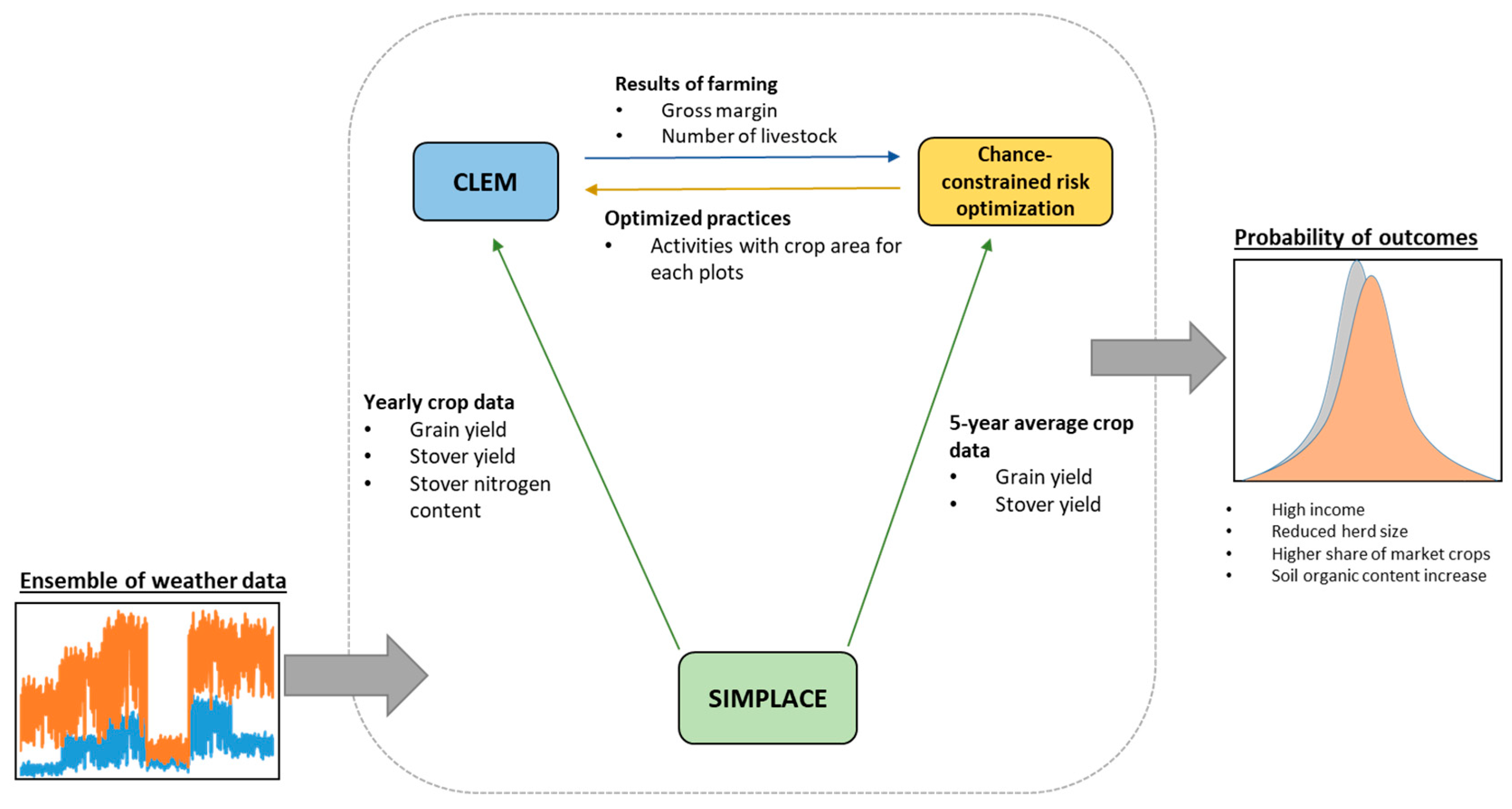
2.5.1. Model Approach Overview
- SIMPLACE: simulates crop grain and biomass yield in response to weather, soil, and management. These simulations are passed to CLEM annually and to the optimization model as yield distributions across all members within a weather scenario;
- CLEM: simulates annual monetary and resource flows and outputs the balances of cash and herd size;
- Optimization model: optimizes resource allocation and the production plan for CLEM.
2.5.2. Crop Model
2.5.3. The Crop Livestock Enterprise Model (CLEM)
2.5.4. Chance-Constrained Risk Optimization Model
- CE = Certainty equivalence of farmer’s gross margin
- E (GM) = Expected gross margin
- RP = Farmer’s risk premium
- subject to:
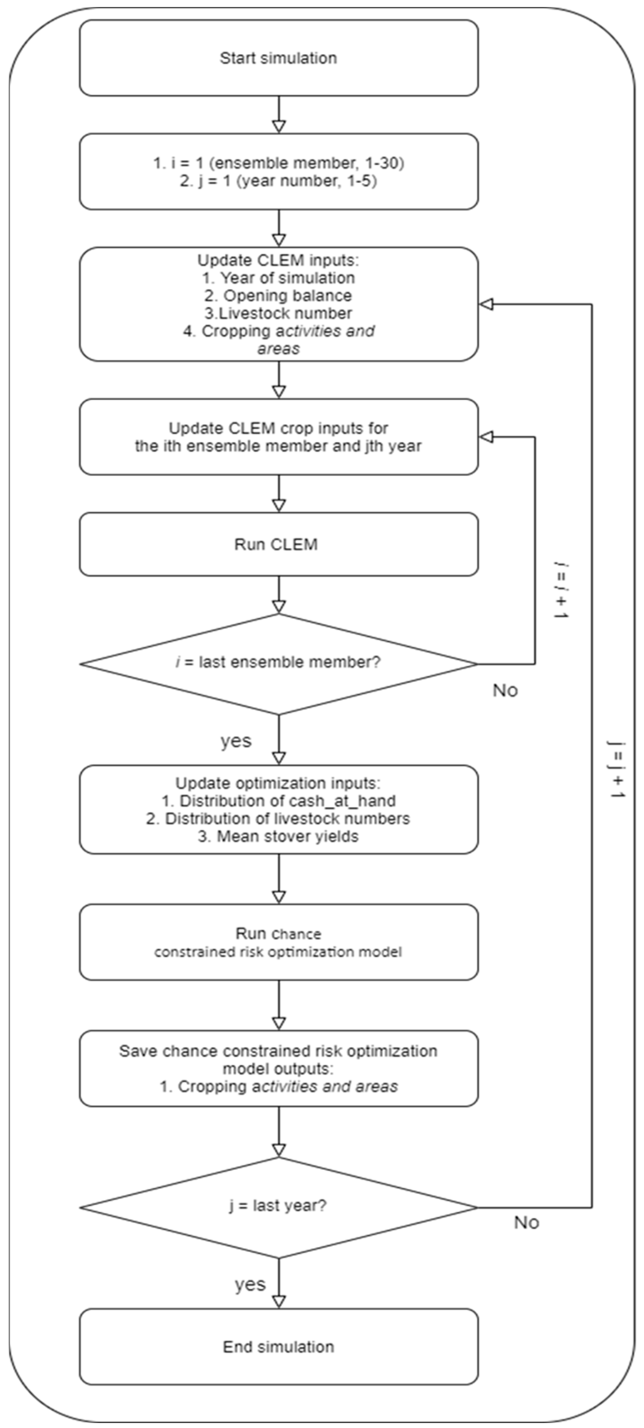
2.5.5. The Integrated Model-Model Coupling
3. Results
3.1. Farm Typology
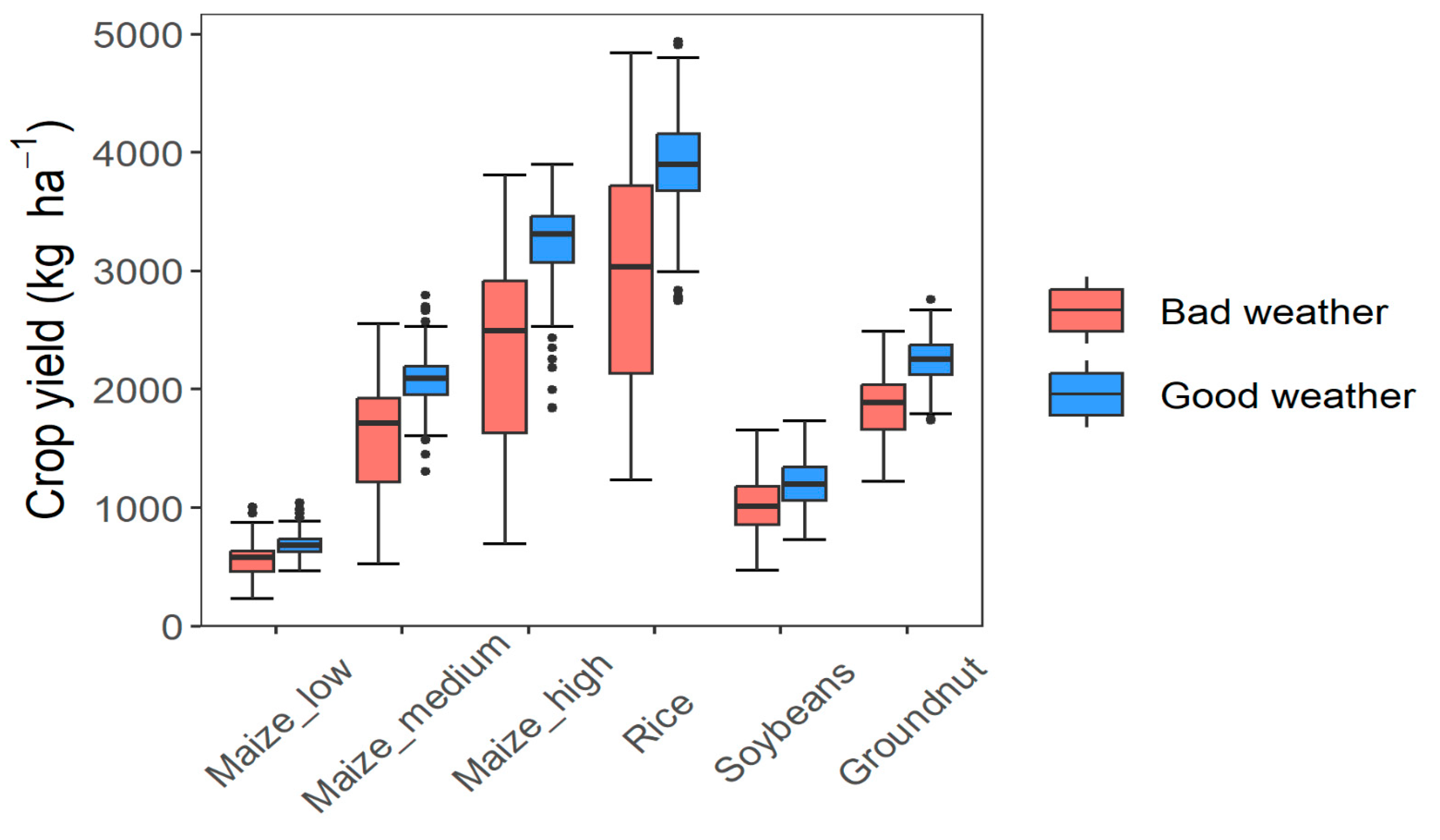
3.2. Crop Yield
3.3. Economic Analysis
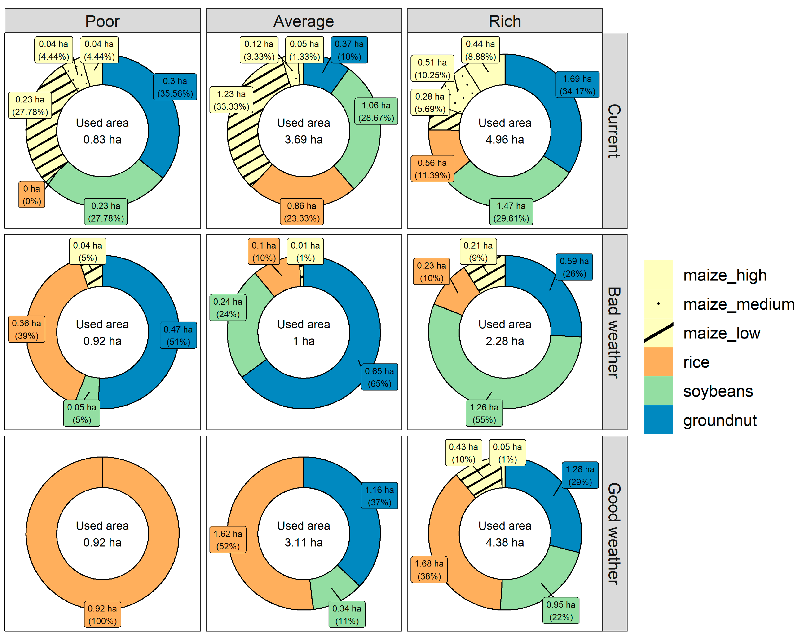
3.4. Optimal Land Allocation
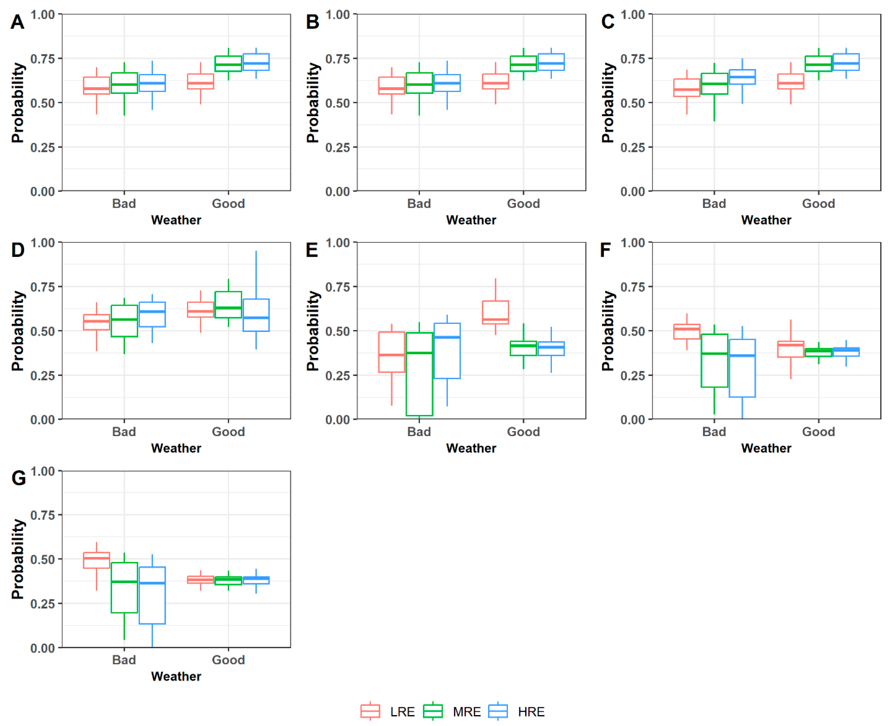
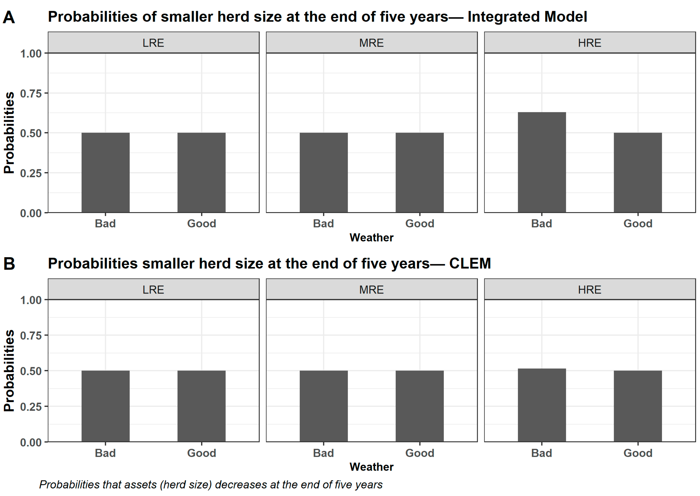
3.5. Effects on Incomes and Assets
4. Discussion
4.1. Relevance of the Integrated Model
4.2. Evaluation of Land Allocation Outputs
4.3. Assessing the Probability of Outcomes
4.4. Inclusion of Risk
4.5. Study Limitations
5. Conclusions
Supplementary Materials
Author Contributions
Funding
Institutional Review Board Statement
Informed Consent Statement
Conflicts of Interest
References
- Pretty, J.; Toulmin, C.; Williams, S. Sustainable Intensification in African Agriculture. Int. J. Agric. Sustain. 2011, 9, 5–24. [Google Scholar] [CrossRef]
- Vanlauwe, B.; Coyne, D.; Gockowski, J.; Hauser, S.; Huising, J.; Masso, C.; Nziguheba, G.; Schut, M.; Van Asten, P. Sustainable Intensification and the African Smallholder Farmer. Curr. Opin. Environ. Sustain. 2014, 8, 15–22. [Google Scholar] [CrossRef]
- Iddrisu, Y.; Abdul-Fatahi, A.; Pokharel, K.; Fred, Y. Sustainable Agricultural Intensification Practices and Rural Food Security: The Case of North Western Ghana. Br. Food J. 2018, 20, 468–482. [Google Scholar] [CrossRef]
- McDonald, C.K.; MacLeod, N.D.; Lisson, S.; Corfield, J.P. The Integrated Analysis Tool (IAT)—A Model for the Evaluation of Crop-Livestock and Socio-Economic Interventions in Smallholder Farming Systems. Agric. Syst. 2019, 176, 102659. [Google Scholar] [CrossRef]
- Pretty, J. The Sustainable Intensification of Agriculture. Nat. Resour. Forum 1997, 21, 247–256. [Google Scholar] [CrossRef]
- Petersen, B.; Snapp, S. What Is Sustainable Intensification? Views from Experts. Land Use Policy 2015, 46, 1–10. [Google Scholar] [CrossRef]
- Gashu, D.; Demment, M.W.; Stoecker, B.J. Challenges and Opportunities to the African Agriculture and Food Systems. Afr. J. Food Agric. Nutr. Dev. 2019, 19, 14190–14217. [Google Scholar] [CrossRef]
- Zhang, T.; van der Wiel, K.; Wei, T.; Screen, J.; Yue, X.; Zheng, B.; Selten, F.; Bintanja, R.; Anderson, W.; Blackport, R.; et al. Increased Wheat Price Spikes and Larger Economic Inequality with 2 °C Global Warming. One Earth 2022, 5, 907–916. [Google Scholar] [CrossRef]
- Aidoo, R.; Mensah, J.O.; Wie, P.; Awunyo-vitor, D. Prospects of Crop Insurance as a Risk Management Tool Among Arable Crop Farmers in Ghana. Asian Econ. Financ. Rev. 2014, 4, 341–354. [Google Scholar]
- Briner, S.; Finger, R. Bio-Economic Modelling of Decisions under Yield and Price Risk for Suckler Cow Farms; European Association of Agricultural Economists: Dublin, Ireland, 2012. [Google Scholar]
- Fahad, S.; Wang, J. Farmers’ Risk Perception, Vulnerability, and Adaptation to Climate Change in Rural Pakistan. Land Use Policy 2018, 79, 301–309. [Google Scholar] [CrossRef]
- Hansen, J.; Hellin, J.; Rosenstock, T.; Fisher, E.; Cairns, J.; Stirling, C.; Lamanna, C.; van Etten, J.; Rose, A.; Campbell, B. Climate Risk Management and Rural Poverty Reduction. Agric. Syst. 2019, 172, 28–46. [Google Scholar] [CrossRef]
- Tang, K.; Hailu, A. Smallholder Farms’ Adaptation to the Impacts of Climate Change: Evidence from China’s Loess Plateau. Land Use Policy 2020, 91, 104353. [Google Scholar] [CrossRef]
- Yin, L.; Boatemaa, A.V.; Mathias, A. Exploring the Risk Exposures of Peasant Farmers in Northern Ghana. Int. J. Innov. Res. Dev. 2016, 5, 93–99. [Google Scholar]
- Huet, E.K.; Adam, M.; Giller, K.E.; Descheemaeker, K. Diversity in Perception and Management of Farming Risks in Southern Mali. Agric. Syst. 2020, 184, 102905. [Google Scholar] [CrossRef]
- Hamsa, K.; Bellundagi, V. Review on Decision-Making under Risk and Uncertainty in Agriculture. Econ. Aff. 2017, 62, 447. [Google Scholar] [CrossRef]
- Faye, B.; Webber, H.; Diop, M.; Mbaye, M.L.; Owusu-Sekyere, J.D.; Naab, J.B.; Gaiser, T. Potential Impact of Climate Change on Peanut Yield in Senegal, West Africa. Field Crops Res. 2018, 219, 148–159. [Google Scholar] [CrossRef]
- Trisos, C.H.; Adelekan, I.O.; Totin, E.; Ayanlade, A.; Efitre, J.; Gemeda, A.; Kalaba, K.; Lennard, C.; Masao, C.; Mgaya, Y.; et al. Climate Change 2022: Impacts, Adaptation and Vulnerability. Change; Cambridge University Press: Cambridge, UK; New York, NY, USA, 2022; ISBN 9781009325844. [Google Scholar]
- Antón, J.; Cattaneo, A.; Kimura, S.; Lankoski, J. Agricultural Risk Management Policies under Climate Uncertainty. Glob. Environ. Chang. 2013, 23, 1726–1736. [Google Scholar] [CrossRef]
- Nafi, E.; Webber, H.; Danso, I.; Naab, J.B.; Frei, M.; Gaiser, T. Can Reduced Tillage Buffer the Future Climate Warming Effects on Maize Yield in Different Soil Types of West Africa? Soil Tillage Res. 2021, 205, 104767. [Google Scholar] [CrossRef]
- Danso, I.; Webber, H.; Bourgault, M.; Ewert, F.; Naab, J.B.; Gaiser, T. Crop Management Adaptations to Improve and Stabilize Crop Yields under Low-Yielding Conditions in the Sudan Savanna of West Africa. Eur. J. Agron. 2018, 101, 1–9. [Google Scholar] [CrossRef]
- Herrero, M.; Grace, D.; Njuki, J.; Johnson, N.; Enahoro, D.; Silvestri, S.; Rufino, M.C. The Roles of Livestock in Developing Countries. Animal 2013, 7, 3–18. [Google Scholar] [CrossRef]
- Pannell, D.J.; Llewellyn, R.S.; Corbeels, M. The Farm-Level Economics of Conservation Agriculture for Resource-Poor Farmers. Agric. Ecosyst. Environ. 2014, 187, 52–64. [Google Scholar] [CrossRef]
- Alary, V.; Corbeels, M.; Affholder, F.; Alvarez, S.; Soria, A.; Valadares Xavier, J.H.; da Silva, F.A.M.; Scopel, E. Economic Assessment of Conservation Agriculture Options in Mixed Crop-Livestock Systems in Brazil Using Farm Modelling. Agric. Syst. 2016, 144, 33–45. [Google Scholar] [CrossRef]
- Binswanger-Mkhize, H.P. Is There Too Much Hype about Index-Based Agricultural Insurance? J. Dev. Stud. 2012, 48, 187–200. [Google Scholar] [CrossRef]
- WFP. The R4 Rural Resilience Initiative. Available online: https://www.wfp.org/r4-rural-resilience-initiative (accessed on 11 January 2023).
- Barbier, B. Induced Innovation and Land Degradation: Results from a Bioeconomic Model of a Village in West Africa. Agric. Econ. 1998, 19, 15–25. [Google Scholar] [CrossRef]
- Louhichi, K.; Flichman, G.; Boisson, J.M. Bio-Economic Modelling of Soil Erosion Externalities and Policy Options: A Tunisian Case Study. J. Bioecon. 2010, 12, 145–167. [Google Scholar] [CrossRef]
- Feola, G.; Sattler, C.; Saysel, K.A.; Saysel, A.K. Simulation Models in Farming Systems Research: Potential and Challenges. In Farming Systems Research into the 21st Century: The New Dynamic; Darnhofer, I., Gibbon, D., Dedieu, B., Eds.; Springer: Dordrecht, The Netherlands, 2012; pp. 281–306. ISBN 9789400745032. [Google Scholar]
- Castro, L.M.; Härtl, F.; Ochoa, S.; Calvas, B.; Izquierdo, L.; Knoke, T. Integrated Bio-Economic Models as Tools to Support Land-Use Decision Making: A Review of Potential and Limitations. J. Bioecon. 2018, 20, 183–211. [Google Scholar] [CrossRef]
- Flichman, G.; Allen, T. Bio-Economic Modeling: State-of-the-Art and Key Priorities; CGIAR: Montpellier, France, 2013. [Google Scholar]
- Wolf, J.; Kanellopoulos, A.; Kros, J.; Webber, H.; Zhao, G.; Britz, W.; Reinds, G.J.; Ewert, F.; de Vries, W. Combined Analysis of Climate, Technological and Price Changes on Future Arable Farming Systems in Europe. Agric. Syst. 2015, 140, 56–73. [Google Scholar] [CrossRef]
- Arribas, I.; Louhichi, K.; Perni, Á.; Vila, J.; Gómez-y-Paloma, S. Modelling Farmers’ Behaviour Toward Risk in a Large Scale Positive Mathematical Programming (PMP) Model. In Advances in Applied Economic Research; Proceedings in Business and Economics; Springer International Publishing AG: Cham, Switzerland, 2017; pp. 625–643. [Google Scholar]
- van Wijk, M.T.; Rufino, M.C.; Enahoro, D.; Parsons, D.; Silvestri, S.; Valdivia, R.O.; Herrero, M. Farm Household Models to Analyse Food Security in a Changing Climate: A Review. Glob. Food Sec. 2014, 3, 77–84. [Google Scholar] [CrossRef]
- Abugri, S.A.; Amikuzuno, J.; Daadi, E.B. Looking out for a Better Mitigation Strategy: Smallholder Farmers’ Willingness to Pay for Drought-Index Crop Insurance Premium in the Northern Region of Ghana. Agric. Food Secur. 2017, 6, 71. [Google Scholar] [CrossRef]
- Abdul-Razak, M.; Kruse, S. The Adaptive Capacity of Smallholder Farmers to Climate Change in the Northern Region of Ghana. Clim. Risk Manag. 2017, 17, 104–122. [Google Scholar] [CrossRef]
- Alhassan, H.; Kwakwa, P.A.; Adzawla, W. Farmers Choice of Adaptation Strategies to Climate Change and Variability in Arid Region of Ghana. Rev. Agric. Appl. Econ. 2019, 22, 32–40. [Google Scholar] [CrossRef]
- Wossen, T.; Berger, T.; Swamikannu, N.; Ramilan, T. Climate Variability, Consumption Risk and Poverty in Semi-Arid Northern Ghana: Adaptation Options for Poor Farm Households. Environ. Dev. 2014, 12, 2–15. [Google Scholar] [CrossRef]
- CGIAR CASCAID—Capacitating African Smallholders with Climate Advisories and Insurance Development. Available online: https://cgspace.cgiar.org/handle/10568/107970 (accessed on 4 July 2022).
- MoFA. Facts & Figures: Agriculture in Ghana, 2020; Ministry of Food & Agriculture: Accra, Ghana, 2021. [Google Scholar]
- MoFA; IFPRI. Ghana’s Soya Bean Market—Market Brief No. 6; Ministry of Food & Agriculture: Accra, Ghana, 2020. [Google Scholar]
- Ghana Statistical Service. Ghana Statical Service PPI Bulletin. Available online: https://www2.statsghana.gov.gh/ppi_bulletin.html (accessed on 23 August 2022).
- Shukla, R.; Agarwal, A.; Gornott, C.; Sachdeva, K.; Joshi, P.K. Farmer Typology to Understand Differentiated Climate Change Adaptation in Himalaya. Sci. Rep. 2019, 9, 20375. [Google Scholar] [CrossRef]
- Gebrekidan, B.H.; Heckelei, T.; Rasch, S. Characterizing Farmers and Farming System in Kilombero Valley Floodplain, Tanzania. Sustainability 2020, 12, 7114. [Google Scholar] [CrossRef]
- Berre, D.; Baudron, F.; Kassie, M.; Craufurd, P.; Lopez-Ridaura, S. Different Ways to Cut a Cake: Comparing Expert-Based and Statistical Typologies to Target Sustainable Intensification Technologies, A Case-Study in Southern Ethiopia. Exp. Agric. 2019, 55, 191–207. [Google Scholar] [CrossRef]
- Kuivanen, K. Dealing with Farming System Diversity in Northern Ghana Typology Approaches Dealing with Farming System Diversity in Northern Ghana: Typology Approaches. Ph.D. Thesis, Wageningen University and Research Centre, Wageningen, The Netherlands, 2015. [Google Scholar]
- Le, S.; Josse, J.; Husson, F. FactoMineR: An R Package for Multivariate Analysis. J. Stat. Softw. 2008, 25, 1–18. [Google Scholar] [CrossRef]
- R Core Team. A Language and Environment for Statistical Computing; R Core Team: Vienna, Austria, 2022. [Google Scholar]
- Kassambara, A. Practical Guide to Principal Component Methods in R: CA, M (CA), FAMD, MFA, HCPC, Factoextra; STHDA: Marseille, France, 2011; Volume 44, ISBN 9788578110796. [Google Scholar]
- van der Wiel, K.; Wanders, N.; Selten, F.M.; Bierkens, M.F.P. Added Value of Large Ensemble Simulations for Assessing Extreme River Discharge in a 2 °C Warmer World. Geophys. Res. Lett. 2019, 46, 2093–2102. [Google Scholar] [CrossRef]
- Deser, C.; Lehner, F.; Rodgers, K.B.; Ault, T.; Delworth, T.L.; DiNezio, P.N.; Fiore, A.; Frankignoul, C.; Fyfe, J.C.; Horton, D.E.; et al. Insights from Earth System Model Initial-Condition Large Ensembles and Future Prospects. Nat. Clim. Chang. 2020, 10, 277–286. [Google Scholar] [CrossRef]
- Hazeleger, W.; Wang, X.; Severijns, C.; Ştefǎnescu, S.; Bintanja, R.; Sterl, A.; Wyser, K.; Semmler, T.; Yang, S.; van den Hurk, B.; et al. EC-Earth V2.2: Description and Validation of a New Seamless Earth System Prediction Model. Clim. Dyn. 2012, 39, 2611–2629. [Google Scholar] [CrossRef]
- Van Der Wiel, K.; Selten, F.M.; Bintanja, R.; Blackport, R.; Screen, J.A. Ensemble Climate-Impact Modelling: Extreme Impacts from Moderate Meteorological Conditions. Environ. Res. Lett. 2020, 15, 034050. [Google Scholar] [CrossRef]
- Vogel, J.; Rivoire, P.; Deidda, C.; Rahimi, L.; Sauter, C.A.; Tschumi, E.; Van Der Wiel, K.; Zhang, T.; Zscheischler, J. Identifying Meteorological Drivers of Extreme Impacts: An Application to Simulated Crop Yields. Earth Syst. Dyn. 2021, 12, 151–172. [Google Scholar] [CrossRef]
- Goulart, H.M.D.; Van Der Wiel, K.; Folberth, C.; Balkovic, J.; Van Den Hurk, B. Storylines of Weather-Induced Crop Failure Events under Climate Change. Earth Syst. Dyn. 2021, 12, 1503–1527. [Google Scholar] [CrossRef]
- Liersch, S.; Tecklenburg, J.; Rust, H.; Dobler, A.; Fischer, M.; Kruschke, T.; Koch, H.; Hattermann, F.F. Are We Using the Right Fuel to Drive Hydrological Models? A Climate Impact Study in the Upper Blue Nile. Hydrol. Earth Syst. Sci. 2018, 22, 2163–2185. [Google Scholar] [CrossRef]
- Faye, B.; Webber, H.; Naab, J.B.; MacCarthy, D.S.; Adam, M.; Ewert, F.; Lamers, J.P.A.; Schleussner, C.F.; Ruane, A.; Gessner, U.; et al. Impacts of 1.5 versus 2.0 °C on Cereal Yields in the West African Sudan Savanna. Environ. Res. Lett. 2018, 13, 034014. [Google Scholar] [CrossRef]
- Meier, E.; Prestwidge, D.; Liedloff, A.; Verrall, S.; Traill, S.; Stower, M. Crop Livestock Enterprise Model (CLEM)—A Tool to Support Decision-Making At. In Proceedings of the Agronomy Australia Conference, Wagga Wagga, Australia, 25–29 August 2019; pp. 25–29. [Google Scholar]
- Webber, H.; Gaiser, T.; Ewert, F. What Role Can Crop Models Play in Supporting Climate Change Adaptation Decisions to Enhance Food Security in Sub-Saharan Africa? Agric. Syst. 2014, 127, 161–177. [Google Scholar] [CrossRef]
- Ewert, F.; Rötter, R.P.; Bindi, M.; Webber, H.; Trnka, M.; Kersebaum, K.C.; Olesen, J.E.; van Ittersum, M.K.; Janssen, S.; Rivington, M.; et al. Crop Modelling for Integrated Assessment of Risk to Food Production from Climate Change. Environ. Model. Softw. 2015, 72, 287–303. [Google Scholar] [CrossRef]
- Wolf, J. User Guide for LINGRA-N: Simple Generic Model for Simulation of Grass Growth under Potential, Water Limited and Nitrogen Limited Conditions; Wageningen University and Research Centre: Wageningen, The Netherlands, 2012. [Google Scholar]
- Addiscott, T.M.; Whitmore, A.P. Simulation of Solute Leaching in Soils of Differing Permeabilities. Soil Use Manag. 1991, 7, 94–102. [Google Scholar] [CrossRef]
- Allen, R.G.; Pereira, L.S.; Raes, D.; Smith, M. FAO Irrigation and Drainage Paper No. 56—Crop Evapotranspiration; FAO: Rome, Italy, 1998. [Google Scholar]
- Gabaldón-Leal, C.; Webber, H.; Otegui, M.E.; Slafer, G.A.; Ordóñez, R.A.; Gaiser, T.; Lorite, I.J.; Ruiz-Ramos, M.; Ewert, F. Modelling the Impact of Heat Stress on Maize Yield Formation. Field Crops Res. 2016, 198, 226–237. [Google Scholar] [CrossRef]
- Webber, H.; Ewert, F.; Kimball, B.A.; Siebert, S.; White, J.W.; Wall, G.W.; Ottman, M.J.; Trawally, D.N.; Gaiser, T. Simulating Canopy Temperature for Modelling Heat Stress in Cereals. Environ. Model. Softw. 2016, 77, 143–155. [Google Scholar] [CrossRef]
- MacCarthy, D.S.; Adiku, S.G.K.; Kamara, A.Y.; Freduah, B.S.; Kugbe, J.X. The Role of Crop Simulation Modeling in Managing Fertilizer Use in Maize Production Systems in Northern Ghana. In Enhancing Agricultural Research and Precision Management for Subsistence Farming by Integrating System Models with Experiments; Wiley: Hoboken, NJ, USA, 2022; pp. 48–68. [Google Scholar]
- Adzawla, W.; Atakora, W.K.; Kissiedu, I.N.; Martey, E.; Etwire, P.M.; Gouzaye, A.; Bindraban, P.S. Characterization of Farmers and the Effect of Fertilization on Maize Yields in the Guinea Savannah, Sudan Savannah, and Transitional Agroecological Zones of Ghana. EFB Bioecon. J. 2021, 1, 100019. [Google Scholar] [CrossRef]
- Bidogeza, J.C.; Berentsen, P.B.M.; De Graaff, J.; Oude Lansink, A.G.J.M. Bio-Economic Modelling of the Influence of Family Planning, Land Consolidation and Soil Erosion on Farm Production and Food Security in Rwanda. J. Dev. Agric. Econ. 2015, 7, 204–221. [Google Scholar] [CrossRef]
- Kim, M.-K.; McCarl, B.A.; Spreen, T.H. Applied Mathematical Programming; Addison-Wesley: Boston, MA, USA, 2013; ISBN 978-0201004649. [Google Scholar]
- Maher, M.J.; Williams, H.P. Model Building in Mathematical Programming, 4th ed.; John Wiley & Sons, Ltd.: Hoboken, NJ, USA, 1999; ISBN 0471997889. [Google Scholar]
- Mccarl, B.A.; Spreen, T.H. Applied Mathematical Programming Using Algebraic Systems; Texas A&M University: College Station, TX, USA, 2005. [Google Scholar]
- Freund, R.J. The Introduction of Risk into a Programming Model. Econometrica 1956, 24, 253. [Google Scholar] [CrossRef]
- Hardaker, J.B.; Huirne, B.M.R.; Anderson, R.J.; Lien, G. Coping with Risk in Agriculture; CABI: Wallingford, UK, 2004; ISBN 0851998313. [Google Scholar]
- Kaiser, M.H.; Messer, D.K. Mathematical Programming for Agricultural, Environmental, and Resource Economics; John Wiley & Sons, Inc.: Hoboken, NJ, USA, 2011; ISBN 9780470599365. [Google Scholar]
- Preckel, P.; Hazell, P.; Norton, R. Mathematical Programming for Economic Analysis in Agriculture. Am. J. Agric. Econ. 1987, 69, 715–716. [Google Scholar] [CrossRef]
- Oxana, K.; van Marcel, A.; Ruud, H. Quadratic Risk Programming for Whole-Farm Planing. In Proceedings of the 2nd International Conference Young Research, Godollo, Hungary, 17–18 October 2002; pp. 1–10. [Google Scholar]
- Laborte, A.G.; Schipper, R.A.; Van Ittersum, M.K.; Van Den Berg, M.M.; Van Keulen, H.; Prins, A.G.; Hossain, M. Farmers’ Welfare, Food Production and the Environment: A Model-Based Assessment of the Effects of New Technologies in the Northern Philippines. NJAS–Wagening. J. Life Sci. 2009, 56, 345–373. [Google Scholar] [CrossRef]
- Nyuor, A.B.; Donkor, E.; Aidoo, R.; Buah, S.S.; Naab, J.B.; Nutsugah, S.K.; Bayala, J.; Zougmoré, R. Economic Impacts of Climate Change on Cereal Production: Implications for Sustainable Agriculture in Northern Ghana. Sustainability 2016, 8, 724. [Google Scholar] [CrossRef]
- Ngeleza, G.K.; Owusua, R.; Jimah, K.; Kolavalli, S. Cropping Practices and Labor Requirements in Field Operations for Major Crops in Ghana: What Needs to Be Mechanized; IFPRI: Accra, Ghana, 2011. [Google Scholar]
- Daadi, B.E.; Latacz-Lohmann, U. Organic Fertilizer Use by Smallholder Farmers: Typology of Management Approaches in Northern Ghana. Renew. Agric. Food Syst. 2021, 36, 192–206. [Google Scholar] [CrossRef]
- Markovi, M.; Šoštaric, J.; Marko, J.; Atilgan, A. Extreme Weather Events Affect Agronomic Practices and Their Environmental Impact in Maize Cultivation. Appl. Sci. 2021, 11, 7352. [Google Scholar] [CrossRef]
- Mueller, N.D.; Gerber, J.S.; Johnston, M.; Ray, D.K.; Ramankutty, N.; Foley, J.A. Closing Yield Gaps through Nutrient and Water Management. Nature 2012, 490, 254–257. [Google Scholar] [CrossRef]
- Leitner, S.; Pelster, D.E.; Werner, C.; Merbold, L.; Baggs, E.M.; Mapanda, F.; Butterbach-Bahl, K. Closing Maize Yield Gaps in Sub-Saharan Africa Will Boost Soil N2O Emissions. Curr. Opin. Environ. Sustain. 2020, 47, 95–105. [Google Scholar] [CrossRef]
- Menapace, L.; Colson, G.; Raffaelli, R. Risk Aversion, Subjective Beliefs, and Farmer Risk Management Strategies. Am. J. Agric. Econ. 2013, 95, 384–389. [Google Scholar] [CrossRef]
- Ullah, R.; Shivakoti, G.P.; Ali, G. Factors Effecting Farmers’ Risk Attitude and Risk Perceptions: THE Case of Khyber Pakhtunkhwa, Pakistan. Int. J. Disaster Risk Reduct. 2015, 13, 151–157. [Google Scholar] [CrossRef]
- Ricome, A.; Affholder, F.; Gérard, F.; Muller, B.; Poeydebat, C.; Quirion, P.; Sall, M. Are Subsidies to Weather-Index Insurance the Best Use of Public Funds? A Bio-Economic Farm Model Applied to the Senegalese Groundnut Basin. Agric. Syst. 2017, 156, 149–176. [Google Scholar] [CrossRef]
- Rusinamhodzi, L.; Corbeels, M.; Van Wijk, M.T.; Rufino, M.C.; Nyamangara, J.; Giller, K.E. A Meta-Analysis of Long-Term Effects of Conservation Agriculture on Maize Grain Yield under Rain-Fed Conditions. Agron. Sustain. Dev. 2011, 31, 657–673. [Google Scholar] [CrossRef]
- Laube, W.; Schraven, B.; Awo, M. Smallholder Adaptation to Climate Change: Dynamics and Limits in Northern Ghana. Clim. Chang. 2012, 111, 753–774. [Google Scholar] [CrossRef]
- Giller, K.E. The Food Security Conundrum of Sub-Saharan Africa. Glob. Food Sec. 2020, 26, 100431. [Google Scholar] [CrossRef]
- Holden, S.; Shiferaw, B. Land Degradation, Drought and Food Security in a Less-Favoured Area in the Ethiopian Highlands: A Bio-Economic Model with Market Imperfections. Agric. Econ. 2004, 30, 31–49. [Google Scholar] [CrossRef]
- Mosnier, C.; Agabriel, J.; Lherm, M.; Reynaud, A. A Dynamic Bio-Economic Model to Simulate Optimal Adjustments of Suckler Cow Farm Management to Production and Market Shocks in France. Agric. Syst. 2009, 102, 77–88. [Google Scholar] [CrossRef]
- Mouysset, L.; Doyen, L.; Jiguet, F.; Allaire, G.; Leger, F. Bio Economic Modeling for a Sustainable Management of Biodiversity in Agricultural Lands. Ecol. Econ. 2011, 70, 617–626. [Google Scholar] [CrossRef]
- Hansen, J.W.; Dinku, T.; Robertson, A.W.; Cousin, R.; Trzaska, S.; Mason, S.J. Flexible Forecast Presentation Overcomes Longstanding Obstacles to Using Probabilistic Seasonal Forecasts. Front. Clim. 2022, 4, 147. [Google Scholar] [CrossRef]
- Becx, G.A.; Mol, G.; Eenhoorn, J.W.; van der Kamp, J.; van Vliet, J. Perceptions on Reducing Constraints for Smallholder Entrepreneurship in Africa: The Case of Soil Fertility in Northern Ghana. Curr. Opin. Environ. Sustain. 2012, 4, 489–496. [Google Scholar] [CrossRef]
- MacCarthy, D.S.; Vlek, P.L.G.; Bationo, A.; Tabo, R.; Fosu, M. Modeling Nutrient and Water Productivity of Sorghum in Smallholder Farming Systems in a Semi-Arid Region of Ghana. Field Crops Res. 2010, 118, 251–258. [Google Scholar] [CrossRef]
- MoFA. Profitability Analysis for Rice. Available online: https://mofa.gov.gh/site/agribusiness/profitability-analysis/381-profitability-analysis-for-rice (accessed on 29 November 2022).
- Mabe, F. Empirical Evidence of Climate Change: Effects on Rice Production in the Northern Region of Ghana. Br. J. Econ. Manag. Trade 2014, 4, 551–562. [Google Scholar] [CrossRef] [PubMed]
- Dietz, T.; Millar, D.; Dittoh, S.; Obeng, F.; Ofori-Sarpong, E. Climate and Livelihood Change in North East Ghana. In The Impact of Climate Change on Drylands in North East Ghana; Kluwer Academic Publishers: Amsterdam, The Netherlands, 2004; Volume 39, pp. 149–172. [Google Scholar]
- Rusinamhodzi, L.; van Wijk, M.T.; Corbeels, M.; Rufino, M.C.; Giller, K.E. Maize Crop Residue Uses and Trade-Offs on Smallholder Crop-Livestock Farms in Zimbabwe: Economic Implications of Intensification. Agric. Ecosyst. Environ. 2015, 214, 31–45. [Google Scholar] [CrossRef]
- Kuivanen, K.S.; Alvarez, S.; Michalscheck, M.; Adjei-Nsiah, S.; Descheemaeker, K.; Mellon-Bedi, S.; Groot, J.C.J. Characterising the Diversity of Smallholder Farming Systems and Their Constraints and Opportunities for Innovation: A Case Study from the Northern Region, Ghana. NJAS—Wagening. J. Life Sci. 2016, 78, 153–166. [Google Scholar] [CrossRef]
- Rufino, M.C.; Thornton, P.K.; Ng’ang’a, S.K.; Mutie, I.; Jones, P.G.; van Wijk, M.T.; Herrero, M. Transitions in Agro-Pastoralist Systems of East Africa: Impacts on Food Security and Poverty. Agric. Ecosyst. Environ. 2013, 179, 215–230. [Google Scholar] [CrossRef]
- Scott, T.J.J.; Baker, C.B. A Practical Way to Select an Optimum Farm, Plan under Risk. Am. J. Agric. Econ. 1972, 54, 657–660. [Google Scholar] [CrossRef]


| Variable | Description | Unit |
|---|---|---|
| Age | Age of the household head | years |
| Cash at hand | Cash at hand at the beginning of the season | GHS |
| Sex | Sex of the household head | - |
| Household size | Number of individuals in the household | - |
| Herd size | Total herd size | - |
| Input costs | Total cost of production inputs | GHS/year |
| Land size | Total land size | ha |
| Main crop | Main crop cultivated by farmers | - |
| Non-farm income | Annual household off farm income | GHS/year |
| Total annual income | Total annual household income | GHS/year |
| Type of Model | Base Year (Year 1) | Subsequent Years (Year 2–5) | ||
|---|---|---|---|---|
| Variable Input | Variable Output | Variable Input | Variable Output | |
| Crop Model |
|
|
|
|
| CLEM model |
|
|
|
|
| Optimization model |
|
|
|
|
| Unit | LRE * | MRE * | HRE * | |
|---|---|---|---|---|
| Adult in household | 1 | 2 | 2 | |
| Children (between 6 and 18) | 1 | 1 | 5 | |
| Children (less than 6) | 0 | 0 | 2 | |
| Remittances | GHS/year | 300 | 338 | 843 |
| Non-farm income | GHS/year | 567 | 1431 | 482 |
| Income from livestock sales | GHS/year | 500 | 441 | 1014 |
| Farm maintenance cost | GHS/year | 150 | 208 | 311 |
| Energy spending cost | GHS/year | 100 | 83 | 170 |
| Household living costs | GHS/year | 120 | 735 | 981 |
| Cash at hand (beginning of the season) | GHS/year | 126 | 1331 | 2393 |
| Average amount of loan | GHS/year | 47 | 1906 | 2536 |
| Loan rate | % per month | 8 | 8 | 8 |
| Input expenses (GHS) | GHS/year | 73 | 663 | 1757 |
| Total land area (hectare) | ha | 0.9 | 4.0 | 6.9 |
| Machinery rental cost (GHS) | GHS/year | 148 | 275 | 462 |
| Cattle | 12 | 6 | 6 | |
| Goat | 2 | 9 | 8 | |
| Sheep | 0 | 3 | 6 | |
| Poultry | 14 | 19 | 18 | |
| Animal supplement costs (GHS) | GHS/year | 12 | 61 | 105 |
| Veterinary visit cost | GHS/year | 0 | 10 | 25 |
| Cost-Benefit Table with Survey Data | Maize-Low | Maize-Medium | Maize-High | Soybean | Upland Rice | Groundnut | |
|---|---|---|---|---|---|---|---|
| Tillage | 1.5 | 3.4 | 5.1 | 2.1 | 3.6 | 4.1 | |
| Fertilization | 6.0 | 20.1 | 20.7 | 5.1 | 4.9 | 0.2 | |
| Sowing | 13.4 | 36.1 | 43.7 | 20.9 | 7.9 | 35.1 | |
| Weeding | 13.7 | 39.2 | 56.6 | 25.0 | 52.3 | 39.3 | |
| Harvesting | 16.4 | 50.5 | 58.9 | 40.5 | 55.9 | 54.6 | |
| Threshing | 4.3 | 5.9 | 21.2 | 8.4 | 5.7 | 12.3 | |
| Total | 55.3 | 155.2 | 206.2 | 102.0 | 130.4 | 145.6 | |
| Input cost (cedi per ha) | Tillage | 88.3 | 146.7 | 254.8 | 151.5 | 377.4 | 267.5 |
| Fertilizer + service | 210.4 | 1234.6 | 2165.6 | 209.6 | 680.1 | 34.5 | |
| Seed + service | 19.4 | 15.5 | 57.2 | 128.5 | 111.6 | 113.1 | |
| Herbicide + service | 77.2 | 121.1 | 398.5 | 110.4 | 185.8 | 157.8 | |
| Harvesting | 13.8 | 27.3 | 70.4 | 28.2 | 26.8 | 40.5 | |
| Threshing | 15.2 | 6.5 | 55.4 | 27.2 | 20.8 | 44.1 | |
| Total | 424.3 | 1551.7 | 3001.9 | 655.3 | 1402.4 | 657.5 | |
| Total variable cost (cedi per ha) | 1530.5 | 4654.7 | 7126.5 | 2696.3 | 4011.2 | 3570.4 | |
| Average yield (kg per ha) | 660.6 | 2162.2 | 3294.7 | 1600.9 | 4229.0 | 3037.3 | |
| Crop price (cedi/kg) | 1.7 | 1.7 | 1.7 | 1.8 | 1.5 | 1.7 | |
| Total revenue (cedi per ha) | 1101.0 | 3603.6 | 5491.2 | 2935.0 | 6343.5 | 5062.2 | |
| Gross contribution (cedi per ha) | 676.7 | 2051.9 | 2489.3 | 2279.6 | 4941.1 | 4404.7 | |
| Contribution margin (cedi per ha) | −429.5 | −1051.1 | −1635.3 | 238.7 | 2332.4 | 1491.9 | |
Disclaimer/Publisher’s Note: The statements, opinions and data contained in all publications are solely those of the individual author(s) and contributor(s) and not of MDPI and/or the editor(s). MDPI and/or the editor(s) disclaim responsibility for any injury to people or property resulting from any ideas, methods, instructions or products referred to in the content. |
© 2023 by the authors. Licensee MDPI, Basel, Switzerland. This article is an open access article distributed under the terms and conditions of the Creative Commons Attribution (CC BY) license (https://creativecommons.org/licenses/by/4.0/).
Share and Cite
Adelesi, O.O.; Kim, Y.-U.; Webber, H.; Zander, P.; Schuler, J.; Hosseini-Yekani, S.-A.; MacCarthy, D.S.; Abdulai, A.L.; van der Wiel, K.; Traore, P.C.S.; et al. Accounting for Weather Variability in Farm Management Resource Allocation in Northern Ghana: An Integrated Modeling Approach. Sustainability 2023, 15, 7386. https://doi.org/10.3390/su15097386
Adelesi OO, Kim Y-U, Webber H, Zander P, Schuler J, Hosseini-Yekani S-A, MacCarthy DS, Abdulai AL, van der Wiel K, Traore PCS, et al. Accounting for Weather Variability in Farm Management Resource Allocation in Northern Ghana: An Integrated Modeling Approach. Sustainability. 2023; 15(9):7386. https://doi.org/10.3390/su15097386
Chicago/Turabian StyleAdelesi, Opeyemi Obafemi, Yean-Uk Kim, Heidi Webber, Peter Zander, Johannes Schuler, Seyed-Ali Hosseini-Yekani, Dilys Sefakor MacCarthy, Alhassan Lansah Abdulai, Karin van der Wiel, Pierre C. Sibiry Traore, and et al. 2023. "Accounting for Weather Variability in Farm Management Resource Allocation in Northern Ghana: An Integrated Modeling Approach" Sustainability 15, no. 9: 7386. https://doi.org/10.3390/su15097386
APA StyleAdelesi, O. O., Kim, Y.-U., Webber, H., Zander, P., Schuler, J., Hosseini-Yekani, S.-A., MacCarthy, D. S., Abdulai, A. L., van der Wiel, K., Traore, P. C. S., & Adiku, S. G. K. (2023). Accounting for Weather Variability in Farm Management Resource Allocation in Northern Ghana: An Integrated Modeling Approach. Sustainability, 15(9), 7386. https://doi.org/10.3390/su15097386