Article

Headland and Field Edge Performance Assessment Using Yield Maps and Sentinel-2 Images

1
Department of Land, Environment Agriculture and Forestry, University of Padova, 35020 Legnaro, Italy
2
Department of Botany and Plant Sciences, University of California, Riverside, CA 92521, USA
*
Author to whom correspondence should be addressed.
Sustainability 2023, 15(5), 4516; https://doi.org/10.3390/su15054516
Submission received: 23 January 2023 / Revised: 1 March 2023 / Accepted: 1 March 2023 / Published: 2 March 2023

Abstract

:
Headland and field edges have a higher traffic frequency compared to the field centre, which causes more compaction. Most repeated compaction is located at the field entrance area and headland during machinery turning and material transporting that takes place during the fertilisation, herbicide laying, and harvesting of fields, which could cause soil structure destruction and yield reduction. In this study, the differences between headland, field edges, and field centre were studied using yield maps and the vegetation indices (VIs) calculated by the Google Earth Engine (GEE). First, thirteen yield maps from 2019 to 2022 were used to measure the yield difference between headland, field edges, and field centre. Then, one hundred and eleven fields from northern Italy were used to compare the vegetation indices (VIs) differences between headland, field edges, and field centre area. Then, field size, sand, and clay content were calculated and estimated from GEE. The yield map showed that headland and field edges were 12.20% and 2.49% lower than the field centre. The results of the comparison of the VIs showed that headlands and field edges had lower values compared to the field centre, with reductions of 4.27% and 2.70% in the normalised difference vegetation index (NDVI), 4.17% and 2.67% in the green normalized difference vegetation index (GNDVI), and 5.87% and 3.59% in the normalised difference red edge (NDRE). Additionally, the results indicated that the yield losses in the headland and field edges increased as the clay content increased and sand content decreased. These findings suggest that soil compaction and structural damage caused by the higher traffic frequency in the headland and field edges negatively affect crop yield.

1. Introduction

Headland and field edges are the areas close to the boundary within arable field margins where the farm equipment turns and moves during field operations [1,2,3]. Many turns were made in headland areas during each field operation of planting, fertilising, and harvesting [4,5]. As a result, the field edges have a higher traffic frequency than the field centre [6,7,8,9,10]. Furthermore, most repeated compaction is localised at the headlands and field edges [10,11,12]. The repeated wheeling in the headland and field edges caused more soil compaction in the top and subsoils [11].
Soil compaction in the headland and field edges leads to the physical and mechanical disturbance of the soil structure and reduces root growth [13,14]. As a result, yields are often lower in the headland and field edges compared to the field centre [3,9,15,16,17,18,19,20]. For example, a five-year field experiment was conducted with sugar beet, wheat, and barley. The headland yield was 26% and 7% less than the field centre in sugar beet and cereals [2]. Similarly, a three-year study of barley and rye showed that soil compaction in the headland was 43.32–44.51% higher than the field interior during germination, as the soil compaction increased to 51.76–53.28% before the harvest. As a result, it reduced the yield of barley and rye by 36.16% and 35.48%, respectively [21]. In addition, some studies mentioned the impact of the headlands on crop performance [3,19,22] and the negative yield effect of traffic-induced soil compaction [23,24]. Although most research has shown that the headland and field edges have a lower yield than the field centre, some research did not find a significant difference in the yield performance in the headland and field edges. For example, a 2-year field experiment on no-till maize and soybean fields showed no significant difference in yield even though the soil bulk density increased due to compaction [25]. Similarly, another study found that the wheat yield in the centre part of the field was 44% to 69% higher compared to the headland. However, the volume of the seed and 1000 kernel weight in the field centre were lower than in the field edges [13].
The previous research found spatial variability between the headland, field edges, and field centre. Many studies discussed the spatial variability in crop performance [3,22]. Yield sampling, yield monitoring, and hand-collecting were used to study the yield spatial variability [2,13,18,21,25]. For example, the yield data were collected to determine the effects of proximity to the field edge on maize and soybean yields using a yield monitor-equipped combine harvester [26]. Similarly, the field and farm-scale yield monitor data were used to estimate the yield difference between headlands and non-headlands from 4145 fields across 63 farms in the US. The results showed that the yields per hectare were 14% and 16% lower in the headland areas for grain and silage [9]. While other researchers also concluded that the yield in the headland area had a 15.6% reduction compared to the field centre area [18]. However, yield increase was also recorded in headland areas [15,18].
Remote sensing and satellite data were used to study within-field variability and crop yield monitoring. The use of remote sensing technology complements traditional within-field spatial variability studies, such as field surveys and monitoring with a combined harvester, by providing a quicker and more extensive study method without sacrificing accuracy. Remote sensing is an additional tool that can cover much larger areas than time-consuming field surveys. Previous studies have utilised remote sensing data [27,28,29] to examine the within-field spatial variability, specifically focusing on the study of within-field variability and biomass in wheat, corn, and alfalfa yields. Additionally, other studies have shown the linear connection between the vegetation indices and the crop yield [27,28,29,30,31,32]. In yield monitoring studies, two common strategies are used for predicting and estimating crop yields. The first strategy involves using biomass and the harvest index, which is a measure of reproductive efficiency calculated as the ratio of grain to total shoot dry matter [29,33,34]. The second strategy involves monitoring crop growth and predicting yields using plant physiological models, remote sensing data, and meteorological data [34,35,36,37]. Vegetation indices have been developed to describe crop growth conditions and estimated yield, such as the normalised difference vegetation index (NDVI), soil adjusted vegetation index (SAVI), green normalized difference vegetation index (GNDVI), and the normalised difference red edge (NDRE) [38,39,40,41,42,43].
Several studies have frequently used satellite data to estimate crop yield, achieving accurate results [10,12,28,44,45,46]. Furthermore, several studies utilised high-resolution satellite data, such as the publicly available Sentinel-2, to implement yield prediction models. Initiated by the European Commission (EC) and the European Space Agency (ESA), Sentinel-2 provides a valuable resource for yield prediction research with its high-resolution recordings [47,48,49,50]. Sentinel-2 systematically provides the global acquisition of high-resolution (10 to 60 m) multispectral images with high revisit frequency (5 days at the equator) and can be easily obtained and analysed through platforms, such as Google Earth Engine (GEE). Sentinel-2 data has already been used to analyse the spatial variability [29,31,39,47,49,51]. This study aims to determine the yield and vegetation index variations between headland, field edges, and field centre by utilising yield maps and Sentinel-2 data instead of solely relying on harvester yield or manual collection methods, as seen in prior studies. The objective of this paper was to investigate the differences between headland, field edges, and field centre using yield maps collected during harvesting and the vegetation indices calculated by the GEE. The specific objectives of this study were to: (I) Quantify the yield difference between the headland, field edges, and centre area of the field; (II) Quantify the VI differences between the headland, field edges, and field centre; (III) Determine the impact of field size on vegetation indices differences between the headland, field edges, and field centre; (IV) Determine the impact of clay and sand content on vegetation index differences between the headland, field edges and field centre.

2. Materials and Methods

The selected fields for this study are located in the Mediterranean climatic zone in northern Italy (Figure 1). The area experiences an average rainfall of 994 mm. The average soil texture of clay, sand, and loam are 29.19%, 30.53%, and 40.28%, respectively, within the study fields. The study area has maize planting dates from March to April, with an average crop age of 160 days from the planting date. In this study, the yield and vegetation indices (VIs) of the headlands, field edges, and field centre were compared by analysing thirteen yield maps collected from one hundred and eleven fields. In addition, the effect of field size, clay, and sand content on the differences in yield and VIs were also examined.

2.1. Yield Maps for the Yield and VI Study

The yield maps used in the study were recorded from the CLAAS combine harvester (Lexion 8000) [52] and forage harvester (Jaguar 900) [53]. The data were collected using these advanced machines manufactured by CLAAS. These machines have been designed to provide accurate and reliable yield measurement data for various crops, making them suitable for yield mapping studies. A detailed description of the years and crops are listed in Table 1. The yield monitoring system installed on the combine harvester was capable of collecting thousands of yield points per hectare, on average, by recording the yield during harvest. Outlier points were removed by removing points in ±3 standard deviations. Filtering was carried out to remove spatial outliers since the delay in data recording was already considered in the yield monitoring calibration performed by the producer. According to this latter point, between 20% and 30% of the points were removed, this is comparable with previously published studies [54]. The yield map of sparse points was interpolated to a raster using the kriging [55] method. Kriging, which uses the ordinary method and the spherical semi-variogram model, was performed through ArcGIS pro (version 2.7.0). Then, the rasters were imported into the GEE. Yield performance and VI differences were analysed in each field’s headland, field edges, and field centre. The specific methodology of the study is listed below.

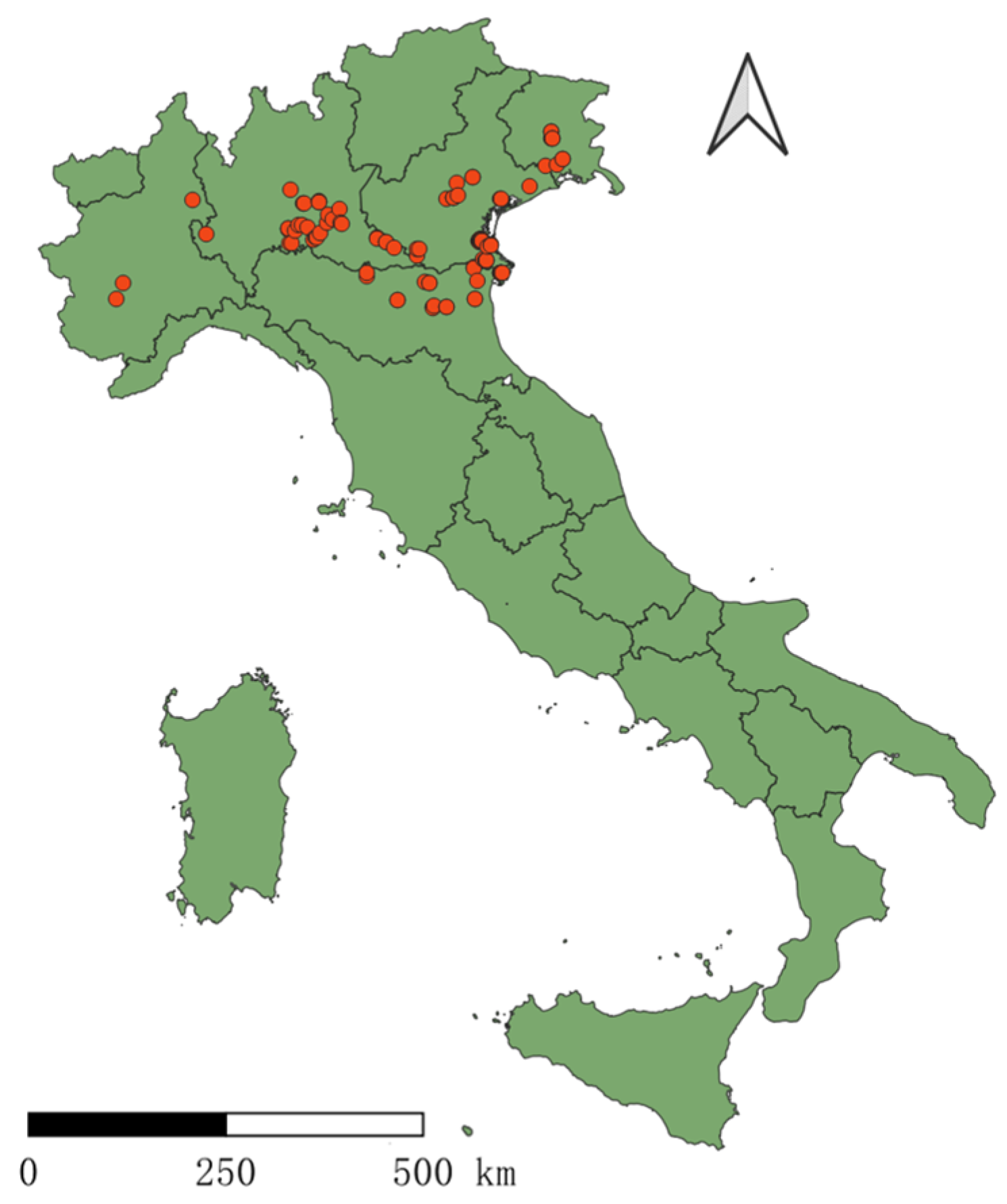
2.2. Field Selection for the VI Study

Fields with different sizes ranged from 2.45 to 38.82 ha, with an average of 13.48 ha. In total, one hundred and eleven fields were selected.
In this study, the focus was on maize, a crucial crop in northern Italy with an average yield of 8 to 10.6 t/ha in the last ten years [56]. The fields were selected using the OneSoil [57] website and EU-CROPMAP 2018 [48,58], which identified the crops grown in different fields for the years between 2016 and 2018 and confirmed the crop type for the year 2018, respectively. Only fields where maize was planted in the same positions (headlands, field edges, and field centres) were considered. The rotation patterns of other crops were not considered. However, the focus on maize was deemed sufficient to achieve the study’s objectives of analysing the differences in yield and vegetation indices between the headlands, field edges, and field centres. The fields selected for this study were chosen based on their regular rectangular shape. The selection was carried out visually, by hand, without specific screening criteria. The regular shape was important for maintaining consistency among the selected fields and provided more disciplined traffic conditions than irregular fields. A certain tolerance for the angle requirements was allowed during the selection process, as it was recognised that obtaining strictly standard fields can be difficult.
Fields were selected while avoiding neighbour obstacles or influencing objects. The obstacles and objects around the field could affect crop performance in the field boundaries. The specific distance for defining a field near trees, rivers, or irrigation canals was not defined. The study only excluded fields that were visibly close to these features. The trees on the edge of the fields may influence the satellite data collection by covering the field with the shade of trees. The presence of neighbouring trees, rivers, or irrigation canals can lead to yield variability in cultivated crops. The study avoided fields that were located too close to these features, as the presence of these features could impact water availability, leading to yield variability. The aim was to choose fields with clean boundaries.

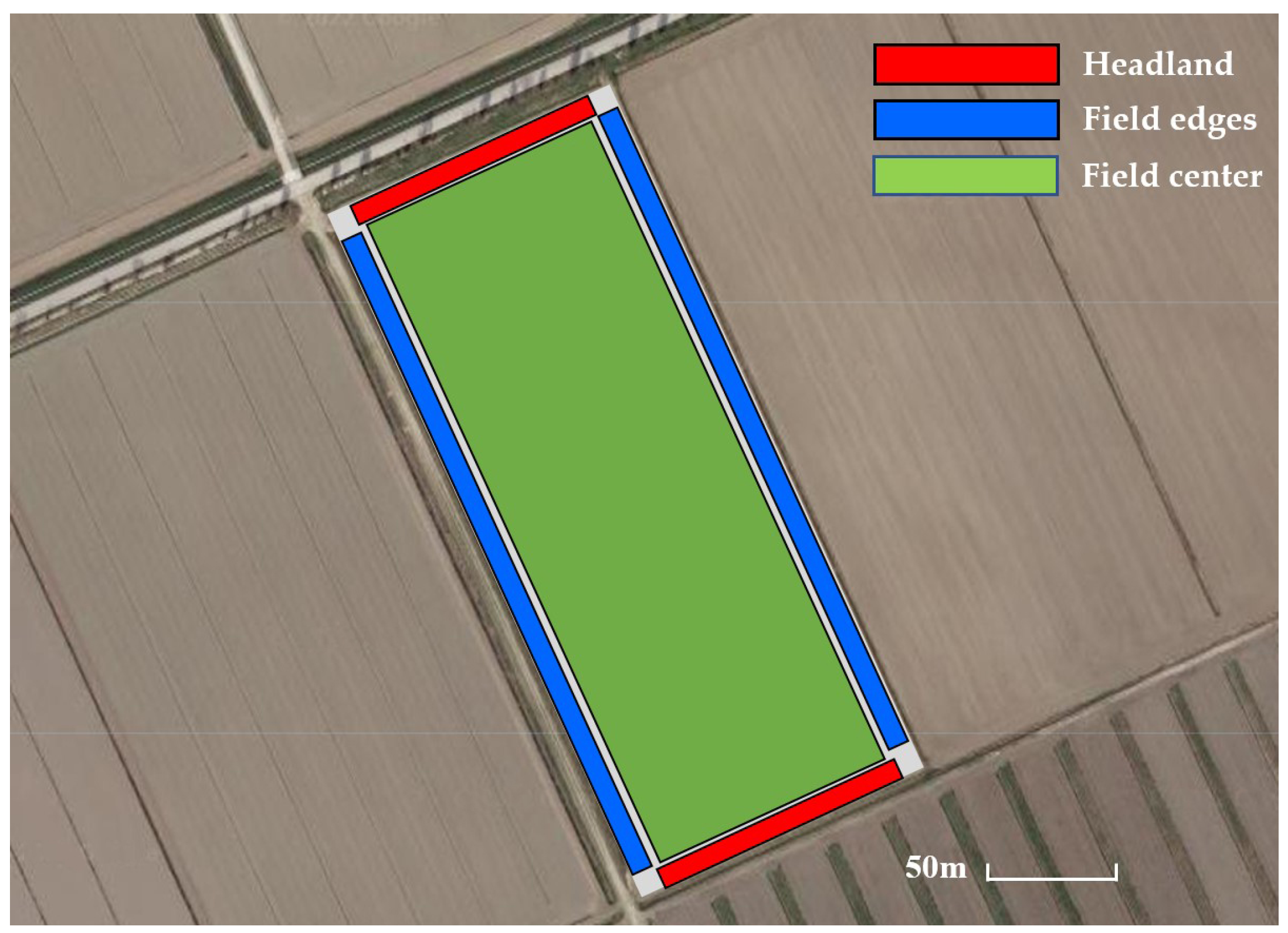
2.3. Field Classification

Each field was divided into three zones using recent and archived Worldview satellite images in the GEE. The field was defined in three parts: headland (red), field edges (blue), and field centre (green), as shown in Figure 2. The width of the headland and field edge areas were not standardised in the study, and there is no general definition for the width of these areas. The headland and field edges were defined based on their respective functions during the farming operation and were visually identified in the yield maps collected from the fields.
  • Headland: The area on the two opposite edges of the field where the farming machinery turns or executes boundary movements during the farming operation (red).
  • Field Edges: The area on the two opposite edges of the field where the farming machinery moves in a linear direction during the farming operation (blue).
  • Field Centre: The central area of the field, excluding the headland and field edges, which is the main farming area (green).
Figure 3 illustrates one sample field with three corresponding zones. The headland and field edges were presented as points of the Sentinel-2 pixels (10 m × 10 m) (headland: red points; field edges: green points). The points were selected from pixels located precisely on the edge of the polygon, as shown in Figure 3. For example, some pixels are half inside the polygon, or others have a gap between the field edges and themselves. The field centre area was presented by a 30 m narrower polygon of the field edges, as the green area shown in Figure 2. The field centre value was automatically calculated by the GEE, which used the mean of all pixels inside the field centre polygon.

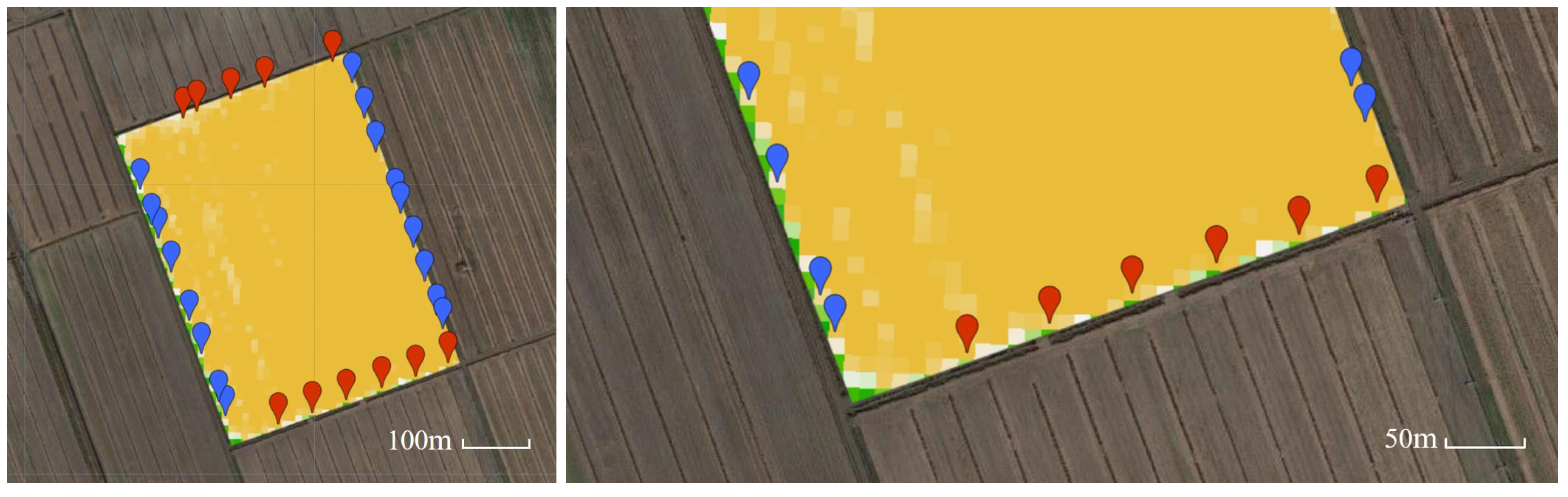
2.4. Yield and VI Data Collection

The yields in the headland, field edges, and field centre of each field were collected when uploading the yield maps. In total, thirteen fields were used in the study using data collected from 2019 to 2022. There were seven silage maize (Zea mays) fields, four triticale (Triticosecale) fields, and two maize (Zea mays) fields, separately. Field sizes ranged from 2.66 to 26.62 ha.
Each year, three dates were selected for the collection of the vegetation index (VI) results from each area (headland, field edges, and field centre) of each field. These dates represented the highest VIs in the Google Earth Engine annually, typically occurring in July to August. This selection allowed for a more thorough analysis of the VIs. The three indices that we used in this study were the normalised difference vegetation index (NDVI), the green normalised difference vegetation index (GNDVI), and the normalised difference red edge (NDRE), as shown in Equations (1)–(3). Three equations were applied through the GEE on filtered Sentinel-2 satellite images, considering the time from 2016 to 2018 and the corresponding zones. The applied filters on Sentinel-2 images include calendar images ranging from May to August. The period corresponds to the summer crop mid-season, which was reported as the most correlated maize yield with vegetation indices from the study area [39,51].
N D V I = N I R R N I R + R
G N D V I = N I R G N I R + G
N D R E = N I R R E N I R + R E
where: NIR is the reflectance at the near-infrared band (band 8, 785–793 nm), R is the reflectance at the red band (band 4, 650–850 nm), G is the reflectance at the green band (band 3, 543–578 nm), and RE is the reflectance at the red edge band (band 5, 698–713 nm) of the Sentinel-2 satellite images.
The temporal resolution might also be influenced by the cloud cover [50]. Therefore, deliberate attention was paid to the effect of cloud cover on data acquisition from the VIs in the study [50]. A cloud percentage filter with a 10% maximum was applied to consider the clear satellite images for further analysis. In addition, a pixel-level cloud filter was applied, taking advantage of the scene classification layer (SCL) provided by Copernicus. The applied filters led to three satellite images from each season with the maximum value within each growing season. Each VI was calculated from each field, the corresponding zones, and all available images. The field size, clay content [59], and sand content [59] of each field were calculated through the GEE using the OpenLandMap which was calculated by the average of the whole field area.

2.5. Statistics

Data collected from each field were used to compare the performance of the headland (H) and field edges (L) with the field centre (C). The field centre served as the control group in order to evaluate the differences. Yield maps for each field were input into the GEE, which was also used to calculate the VIs. The three maximum values in the headland, field edges, and field centre for each field and each year were used for analysis. Value differences between the headland, field edges, and field centre were compared using H/C, L/C, 1-H/C, and 1-L/C. One-way ANOVA and t-tests (at a significance level of 5%) were performed to assess the differences between the three zones for the study fields. The normal distribution of each data group was verified prior to the analysis. The Pearson test (at a significance level of 0.05) was used to quantify the linear association with the field size, clay content, and sand content in the headland, field edges, and field centre.

3. Results

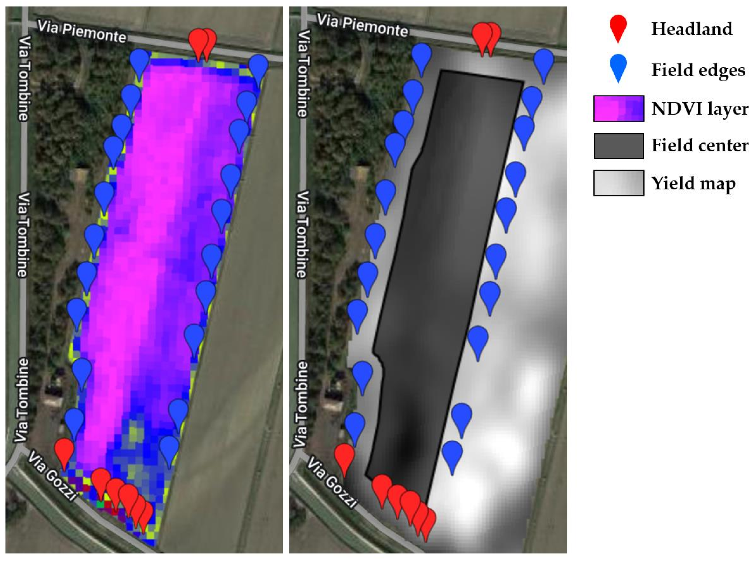
3.1. Comparision between the Yield Map and the VI Results

The VI (NDVI) map (left) and yield map (right) are shown in Figure 4 as an example. The red points represent the headland, and the blue points represent the field edges selected based on the appropriate methodology chosen by the location of the field edges. It is worth noting that only two points in the northern headland are accurately located on the edge of the field. The black polygon inside the field (shown in the right figure as the field centre. The grayscale image is the yield map imported into the GEE after the kriging.
The yield map results of the selected fields are listed in Table 1. The specific year of the field, crop type, field size, and the yield in each location, as well as the difference between the headland (H) with the field centre (C), and the field edges (L) with the field centre (C) are listed. The result showed that the average yield was 12.20% and 2.49% lower in the headland and field edges, respectively, than in the field centre. Among all of the fields, eleven fields showed a lower yield in the headland and field edges than in the field centre. Field numbers 5 and 9 had the highest yield in the field edges rather than in the field centre. Among all fields, nine fields showed significant differences between the headland, field edges, and field centre. However, field numbers 5, 6, and 9 showed no significant difference between the headland and field centre, or the field edges and field centre at a 0.05 confidence level.
The comparison of the VI results within each group are shown in Table 2. The NDVI, GNDVI, and NDRE results showed that the headland and field edges had a lower value than the field centre in most fields. The value difference between the headland and field centre (1-H/C) is higher than the difference between the field edges and field centre (1-L/C) in most fields. The average result among all of the fields showed that the headland and field edges were 12.97% and 5.89% lower than the field centre in the NDVI, 10.55% and 5.11% lower in the GNDVI, and 16.27% and 7.03% lower in the NDRE.
Smaller values were found at the headland and field edges compared to the field centre for both yield and VI result. The VI results showed the same trend and value differences as the yield data. However, the NDVI and GNDVI slightly underestimated the difference in values, and the NDRE slightly overestimated the difference, respectively.

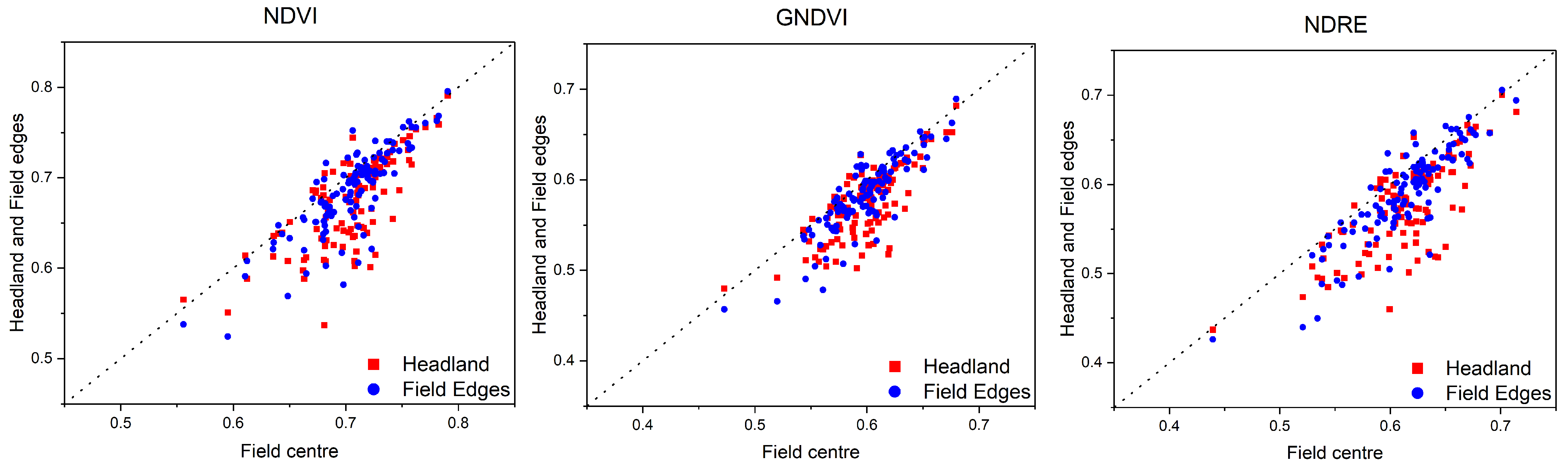
3.2. Comparision of the VIs between the Headland, Field Edges, and Field Centre

The VIs in the headland, field edges, and field centre are shown in Table 3. The results showed that the headland has the lowest VI and the field edges have lower VIs than the field centre in the NDVI, GNDVI, and NDRE. The mean value of the NDVI and GNDVI showed a significant difference between the field centre with the headland and field edges at a 0.05 level. However, there was no significant difference between the headland and field edges. As for the results of the NDRE, the three positions all show significant differences compared with each other at a 0.05 level.
The comparisons between the field centre with the headland and field edges in the NDVI, NDRE, and GNDVI are shown in Figure 5. The red points represent the value of the headland and field centre, and the blue points represent the value of the field edges and field centre. Among all 111 fields, 96/111 (86.5%) of the headland and 93/111 (83.8%) of the field edges were lower than the field centre in the NDVI. Furthermore, 96/111 (86.5%) of the headland and 94/111 (84.7%) of field edges were lower than the field centre in the GNDVI. As for the NDRE, 103/111 (92.8%) and 97/111 (87.4%) of the headland and field edges, respectively, were lower than the field centre.

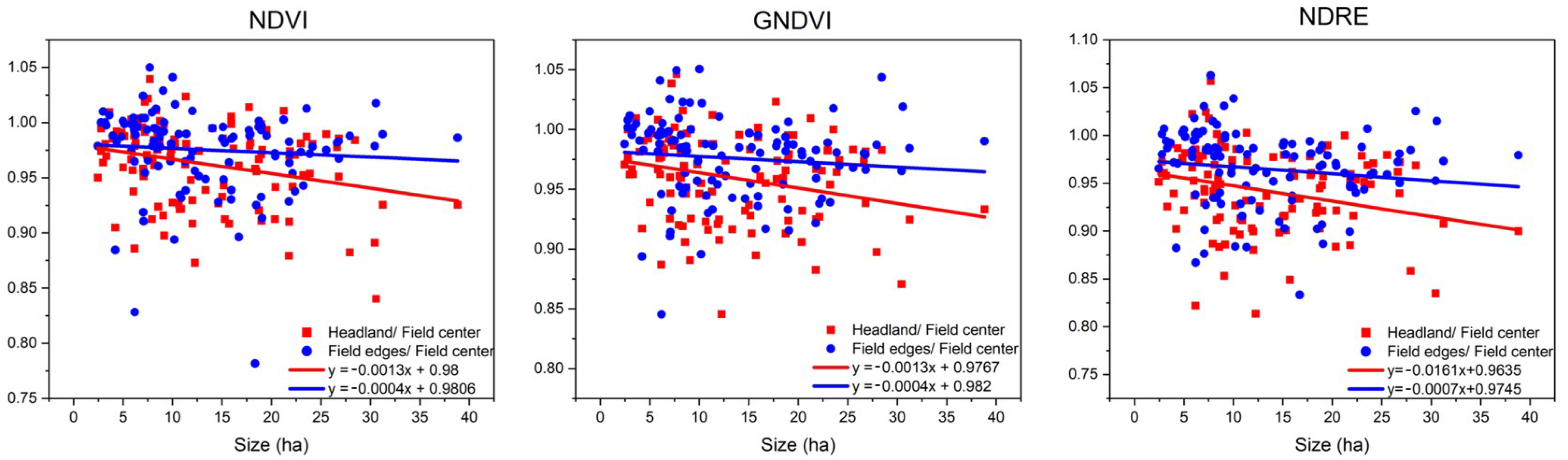
3.3. The Impact of the Field Size on the Vegetation Index Differences between the Three Areas

Figure 6 shows the correlation between the field size and VI difference (%) of the headland and field edges with the field centre (H/C and L/C). The results showed that the H/C and L/C increased with the field size. The red points represent the value of the headland/field centre. The blue points represent the field edges/ field centre. The red and blue lines are the trend lines, respectively.
The headland/field centre trend line (red line) showed a steeper slope in all three VIs than the field edges/field centre (blue line). As shown in Figure 6 he value differences between the headland, field edges, and field centre increased along with the field size. No significant correlations were found between the headland, field edges, and field centre in the NDVI, GNDVI, and NDRE. The p-value was higher than 0.05 and lower than 0.169 in the six comparisons of H/C and L/C in the NDVI, GNDVI, and NDRE

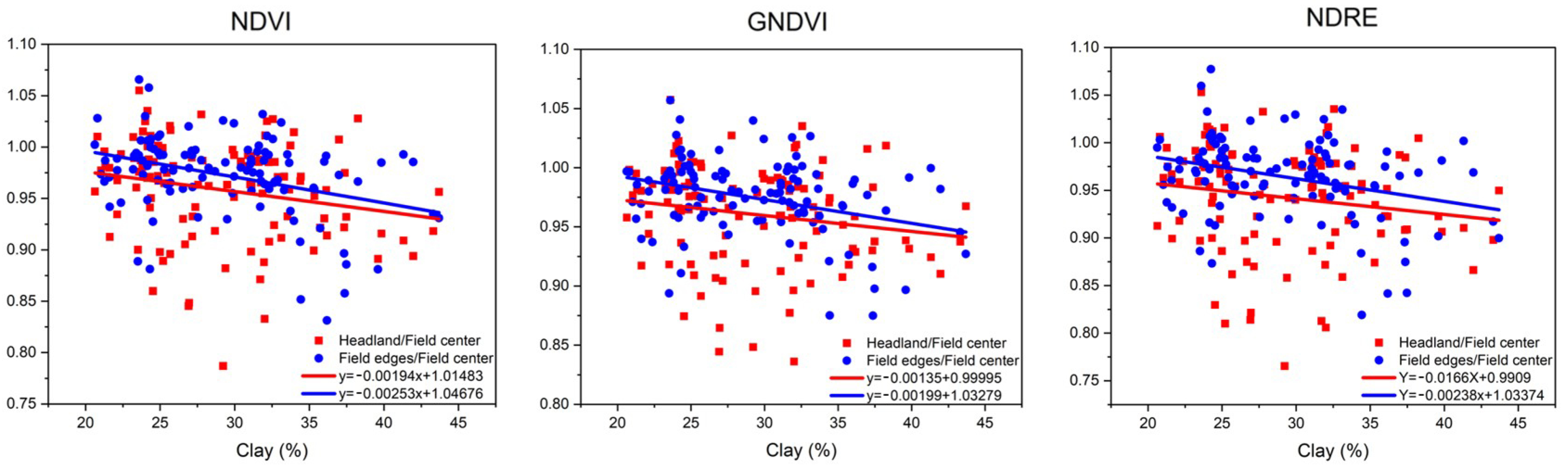
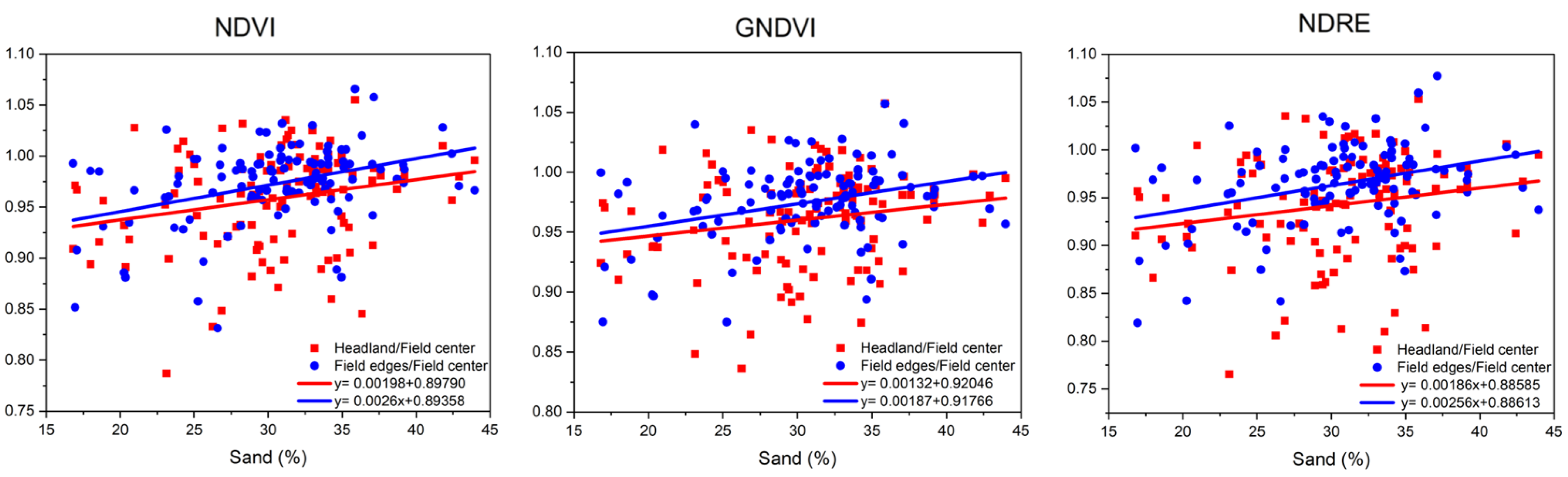
3.4. The Impact of the Soil Texture on Vegetation Index Differences between the Three Areas

Figure 7 shows the correlation between the clay content and VI differences (%) of the headland (red point, H/C) and field edges (blue point, L/C) with the field centre. The red points represent the value of the headland/ field centre. The blue points represent the field edges/ field centre. The red and blue lines are the trend lines, respectively. The field’s clay content range was from 20.63% to 43.70%. The results showed that the value differences between the headland and field edges with the field centre increased as the clay content decreased. Furthermore, the value differences between the headland and field edges with the field centre narrowed as clay content increased.
Significant correlations were found between the headland, field edges, and field centre in the NDVI, GNDVI, and NDRE. Except for the H/C in the GNDVI and NDRE, which was 0.069 and 0.086, respectively, there were no significant correlations with the clay content in the field. The p-value was lower than 0.05 in most of the comparisons of H/C and L/C in the NDVI, GNDVI and NDRE.
Figure 8 shows the correlation between the sand content and VI differences (%) of the headland (red point, H/C) and field edges (blue point, L/C) with the field centre. The value differences between the headland, field edges, and field centre were calculated from the average of three years from 2016 to 2018. The red points represent the value of the headland/ field centre. The blue points represent the field edges/ field centre. The red and blue lines are the trend lines, respectively.
The sample field’s sand content ranges from 16.81% to 48.62%. The results showed that the value differences decreased between the headland and field edges with the field centre, as the sand content increased. Furthermore, the value differences between the headland and field edges became larger as the sand content increased.
Significant correlations were found between the headland, field edges, and field centre in the NDVI, GNDVI, and NDRE. Except for the H/C in the GNDVI (0.063), there were no significant correlations with the clay content in the field. The p-value was lower than 0.05 with regards to all other comparisons of the H/C and L/C in the NDVI, GNDVI, and NDRE.
In summary, yield and VI results both showed significant differences between the headland, field edges, and field centre at a 0.05 confidence level. The yield map results showed that the headland and field edges were 12.20% and 2.49% lower than the field centre in 13 fields. The VI results showed that the headland and field edges were 4.27% and 2.70% lower in the NDVI, 4.17% and 2.67% lower in the GNDVI, and 5.87% and 3.59% lower in the NDRE of 111 fields, respectively. The yield losses in the headland and field edges increased along with the field size and with the increase in clay content, as well as with the decrease in sand content.

4. Discussion

4.1. Yield and VI Differences between the Headland, Field Edges, and Field Centre

In this study, we found similar results to previous studies [3] that showed that the headlands (turning areas) had lower yields compared to the field centre (mid-field area) [17,18,19,20]. These results showed that the headlands had lower yields than the non-headland areas. However, the exact magnitude of the yield differences between the headlands and field centres varied among previous studies. In previous studies, average yield reduction ranged from 7–45% for cereals, 10% for potatoes, and 26% for sugar beet [2,9,16,19,60].
The field’s location and climate zone may play a role in the variability of these results, as different areas may have different environmental conditions that could impact crop growth and yield. Similarly, field size could also impact the results, as larger fields may have less headland area compared to smaller fields. Further research could examine these factors to better understand how they impact the relationship between the headland yield and field centre yield.
However, each field has its unique soil conditions, climate characteristics of different regions, specific annual weather conditions, and manual operation experience. For example, the traffic conditions will differ because of each field’s implement size, working widths, and turning methods. It is important to note that the results of this study may not be representative of all fields, as the results were specific to the sample fields selected for the study. That could explain why not all fields had lower yields or VIs in the headland and field edges. The results of this study are consistent with previous findings that show that the headland and field edges tend to experience more compaction due to the increased traffic during farming operations, leading to substantial reductions in crop yields [61,62]. This has been previously reported in other studies [25,63,64]. The headland and field edges should have a lower yield because of more machine traffic than in the field centre if all the fields have the same working conditions and agronomy. In addition to the soil compaction, yield loss in the headland and field edges may also reflect soil erosion, planter and fertiliser efficiency, within-field variability, edge-feeding of weeds and pests (birds, rodents, and deer), and competition for light, water, and nutrient resources with adjacent obstacles.
More soil compaction in headland and field edges: During each field operation, there is more traffic in the headland and field edges than in the field centre. Most repeated compaction is localised at the field entrance area and in the headlands [10,11,12]. The field edges have a higher traffic frequency than the field centre [6,7]. Traffic in the headland and field edges will cause more compaction both in the topsoil and subsoil [6], which destroys the soil structure, increases soil erosion [65,66,67,68], and causes yield reduction [69,70,71].
Planter and fertiliser efficiency: Skips and overlaps can happen in the headland during seeding and fertilising. Skips can reduce the sown area and crop uniformity, which reduces the yield [61]. The overlaps (doubling inputs) could negatively affect the crop due to a reduced stand uniformity within the field. Overlaps can result in excessive plant densities, which could be favourable for disease development. It also could have a negative impact on production applications, such as difficulty determining the optimal spraying time for uneven maturity. Overlaps can also lead to lodging, making harvesting difficult [72].
Edge-feeding of insects and weeds: A high number of weeds in the field can negatively impact neighbouring crops by vying for light, nutrients, and water, leading to a decrease in the yield of the headland and field edges [73,74]. However, the VI data were collected at a time when the crop had reached the highest index, a few months before the main crop product was harvested. So this reason may be less influential in this study.
Competition for light, water, and nutrient resources with adjacent obstacles: The obstacles and objects around the field could affect crop performance in field boundaries, such as neighbouring trees, rivers, or irrigation canals. Trees that grow on the edge of fields may influence crop growth by shading the field. Additionally, rivers or irrigation canals around the field could cause yield spatial variability in cultivated crops due to the available water variability. As in this study, fields surrounded by trees and rivers have been avoided, as described in the methodology. So, the study removed this reason for the yield and VI decreases.
Methodology of the data collection: The pixel size is 10×10 m which was selected from the GEE. It is quite a large area if the field is not of a large size. The previous study even divided the headland area into three areas: field edge, turning, and transition areas to study the performance difference between the three [22]. So, it could be possible to find a higher value difference between the headland, field edges, and field centre if the resolution is higher than 10 × 10 m. Additionally, not all of the pixels selected during this study were parallel-selected with the field boundaries, as shown in Figure 9. The purple nails were the data collection points, which means that the results underestimated the yield reduction in the headland and field edges because the pixels were more distant from the field boundaries, rather than located precisely on the field boundaries. So it means that if the resolution of the pixels was higher than 10 × 10 m, as in this study, more yield losses or lower VIs could be found in future research studies. Moreover, in future studies, these could be tested by comparing the parallel and non-parallel fields.
In general, researchers mentioned that the reduced headland yields were due to factors, such as compaction caused by the movement of agriculture machines, water, and light competition from woods and hedgerows, weed ingress, and destruction caused by animals [17]. Although each of the reasons above could influence the yield in the headland, most research considered traffic and compaction to be the predominant factors causing the headland yield reduction [2,3,17,75].
This study aimed to know how much yield is lost in the headland and field edges based on the yield and VI maps. Concerning the interpretation of the crop behaviour, more in-depth information might be gained by implementing hyperspectral data and higher-resolution data [76]. Using higher-resolution data could provide a more detailed understanding of crop behaviour. Smaller pixels can capture the true value of the headlands and field edges more accurately than larger pixels, providing a more precise representation. In addition to enhancing geometric accuracy, high-resolution imagery also offers the advantage of advanced spectral resolution, including increased numbers of spectral bands and greater spectral bandwidths, which can facilitate improved interpretation of crop behaviour. By way of example, the application of the PRISMA satellite (experimental satellite from the Italian Space Agency) may improve such a classification thanks to 240 bands from 400–2500 nm with a spatial resolution of 5 m (panchromatic). Unfortunately, the PRISMA satellite is still in experimental stages and cannot be used for wide-area land monitoring. However, it is worth noting that such an approach could increase the effort for data analysis. Furthermore, it might reduce the potential interest and applicability in farm practice. The farm could determine a better strategy using the yield and VI map results if they are convenient enough. Then, better decisions could be made by increasing potential production, planting other crops, or reducing fertility or other input, such as assessing the economic benefits if the same amount of fertiliser needs to be laid in the headland and field edges. If the crop performance of the headlands is affected by machine traffic, it may indicate that headland traffic management may need to be improved to protect the production capacity of these areas. As for the yield losses in the headland and field edges, potential solutions include optimal path planning [4] or controlled farming traffic (CTF) [77,78,79], which could reduce the impact of compaction of the field. However, optimal path planning could be challenging to implement when the width of the equipment is different, such as planters, harvesters, and fertiliser application equipment [9].

4.2. Impact of the Field Size and Soil Texture

The study found that the VI differences became larger between the headland and field edges with field centre as the field size increased. The value differences were smaller in the smaller fields (less than 10 ha), mainly between 95% and 102.5%. The value differences were higher in the larger fields (more than 10 ha), mainly between 90% and 100%. However, no significant correlations were found between the headland, field edges, and field centre in the NDVI, GNDVI and NDRE.
The results showed that the value difference between the headland and field edges and between the field edges and field centre increased with the clay content. Conversely, the difference was reduced as the sand content increased. This phenomenon emphasised the effect of soil compaction on VI reduced yield losses in areas of headland and field edges because of the effect of the soil texture on soil compaction. The plastic limits (lower plastic limit and liquid limit) are important soil properties that can influence the soil’s mechanical behaviour, which is highly related to the clay content [80]. Fields with a higher clay content were considered more sensitive to soil compaction [81,82]. Some researchers assumed yield losses due to the soil compaction of 8% for soils with >40% clay and 4% for soils with 15–25% clay and that yield losses for lighter soils are negligible [83]. Conversely, Sandy soils are often considered structurally inert because of their massive structure and the absence of shrink-swell properties [77] and cause less compaction by the machine traffic [84,85]. The slope of the fields could have influenced the results. However, the research area was located in a plain region with uniform slopes, so the difference between the slopes was minimal. Based on the USGS global digital elevation model, the average slope in the low plain in northern Italy is 0.27%. Thus, this aspect was not analysed in the study. It is worth noting that the relationship between the headlands, field edges, and field centres could be further analysed in future studies.

5. Conclusions

This study used yield maps and vegetation indices (VIs) calculated using the Google Earth Engine (GEE) to compare the differences in yield and VIs between the headland, field edges, and field centre. The results indicated that the headland and field edges had lower yields and VIs compared to the field centre, with the headland yields being 12.20% lower and field edge yields being 2.49% lower than the field centre. The VI results also showed that the headland and field edges were lower by 4.27% to 5.87% compared to the field centre for the NDVI, GNDVI, and NDRE. The differences between the headland, field edges, and field centre were found to increase with the increasing clay content and decrease with the increasing sand content. However, no significant correlations were found between the headland, field edges, and field centre in terms of field size.
The study’s results suggest that optimizing machine traffic management during field operations could reduce yield losses in the headland and field edges, while considering factors, such as soil organic content, field slope, and crop type. These findings have significant implications for the farming industry and provide decision-makers with valuable insight to improve yields and increase profitability. Further research in this field is necessary to understand the complex interplay between crop performance and environmental factors.

Author Contributions

Conceptualisation, F.M. and A.K.; methodology, K.L., A.K. and M.S.; validation, K.L., A.K. and M.S.; formal analysis, K.L.; data curation, K.L. and M.S.; writing—original draft preparation, K.L.; writing—review and editing, A.K. and F.M.; visualisation, F.M.; supervision, A.K. and F.M.; project administration, L.S.; funding acquisition, L.S. All authors have read and agreed to the published version of the manuscript.

Funding

The research activity of the PhD candidate Kaihua Liu is financially supported by a grant from the China Scholarship Council (CSC). This study was carried out within the Agritech National Research Centre and received funding from the European Union Next-GenerationEU (PIANO NAZIONALE DI RIPRESA E RESILIENZA (PNRR)—MISSIONE 4 COMPONENTE 2, INVESTIMENTO 1.4—D.D. 1032 17/06/2022, CN00000022). This manuscript reflects only the authors’ views and opinions, neither the European Union nor the European Commission can be considered responsible for them.

Data Availability Statement

Data presented in this study are available on request from the corresponding author.

Conflicts of Interest

The authors declare no conflict of interest.

References

  1. Boatman, N.D. Field Margins: Integrating Agriculture and Conservation. In Proceedings of the FAO Symposium, Coventry, UK, 18–20 April 1994. [Google Scholar]
  2. Sparkes, D.L.; Jaggard, K.W.; Ramsden, S.J.; Scott, R.K. The Effect of Field Margins on the Yield of Sugar Beet and Cereal Crops. Ann. Appl. Biol. 1998, 132, 129–142. [Google Scholar] [CrossRef]
  3. Wilcox, A.; Perry, N.H.; Boatman, N.D.; Chaney, K. Factors Affecting the Yield of Winter Cereals in Crop Margins. J. Agric. Sci. 2000, 135, 335–346. [Google Scholar] [CrossRef]
  4. Bochtis, D.D.; Vougioukas, S.G. Minimising the Non-Working Distance Travelled by Machines Operating in a Headland Field Pattern. Biosyst. Eng. 2008, 101, 1–12. [Google Scholar] [CrossRef]
  5. Jin, J.; Tang, L. Optimal Coverage Path Planning for Arable Farming on 2D Surfaces. Trans. ASABE 2010, 53, 283–295. [Google Scholar] [CrossRef]
  6. Rodrigues, C.K.; Da Silva Lopes, E.; M’ller, M.M.L.; Genú, A.M. Variabilidade Espacial Da Compactação de Um Solo Submetido Ao Tráfego de Harvester e Forwarder. Sci. For. Sci. 2015, 43, 387–394. [Google Scholar]
  7. Scott, D.I.; Tams, A.R.; Berry, P.M.; Mooney, S.J. The Effects of Wheel-Induced Soil Compaction on Anchorage Strength and Resistance to Root Lodging of Winter Barley (Hordeum vulgare L.). Soil Tillage Res. 2005, 82, 147–160. [Google Scholar] [CrossRef]
  8. Spekken, M.; de Bruin, S. Optimized Routing on Agricultural Fields by Minimizing Maneuvering and Servicing Time. Precis. Agric. 2013, 14, 224–244. [Google Scholar] [CrossRef]
  9. Sunoj, S.; Kharel, D.; Kharel, T.; Cho, J.; Czymmek, K.J.; Ketterings, Q.M. Impact of Headland Area on Whole Field and Farm Corn Silage and Grain Yield. Agron. J. 2021, 113, 147–158. [Google Scholar] [CrossRef]
  10. Duttmann, R.; Brunotte, J.; Bach, M. Spatial Analyses of Field Traffic Intensity and Modeling of Changes in Wheel Load and Ground Contact Pressure in Individual Fields during a Silage Maize Harvest. Soil Tillage Res. 2013, 126, 100–111. [Google Scholar] [CrossRef]
  11. Duttmann, R.; Schwanebeck, M.; Nolde, M.; Horn, R. Predicting Soil Compaction Risks Related to Field Traffic during Silage Maize Harvest. Soil Sci. Soc. Am. J. 2014, 78, 408–421. [Google Scholar] [CrossRef]
  12. Godwin, R.J.; Miller, P.C.H. A Review of the Technologies for Mapping Within-Field Variability. Biosyst. Eng. 2003, 84, 393–407. [Google Scholar] [CrossRef] [Green Version]
  13. Gaženja, U. The decrease of wheat yield on the plot edges—Headlands due to soil compaction. In Proceedings of the 47th International Symposium, Actual Tasks on Agricultural Engineering, Opatija, Croatia, 5–7 March 2019; pp. 97–106. [Google Scholar]
  14. Szatanik-Kloc, A.; Horn, R.; Lipiec, J.; Siczek, A.; Boguta, P. Initial Growth and Root Surface Properties of Dicotyledonous Plants in Structurally Intact Field Soil and Compacted Headland Soil. Soil Tillage Res. 2019, 195, 104387. [Google Scholar] [CrossRef]
  15. Boatman, N.D.; Sotherton, N.W. Agronomic Consequences and Costs of Managing Field Margins for Game and Wildlife Conservation. In Proceedings of the Conference on Environmental Aspects of Applied Biology, York, UK, 19–21 September 1988. [Google Scholar]
  16. De Snoo, G.R. 13 Cost-Benefits of Unsprayed Crop Edges in Winter Wheat, Sugar Beet and Potatoes. In Unsprayed Field Margins: Implications for Environment, Biodiversity and Agricultural Practice; British Crop Protection Council: Farnham, UK, 1994; Volume 167. [Google Scholar]
  17. Speller, C.S.; Cleal, R.A.E.; Runham, S.R. A Comparison of Winter Wheat Yields from Headlands with Other Positions in Five Fen Peat Fields; Monographs-British Crop Protection Council: Farnham, UK, 1992; Volume 47. [Google Scholar]
  18. Cook, S.K.; Ingle, S. The Effect of Boundary Features at the Field Margins on Yields of Winter Wheat. Asp. Appl. Biol. 1997, 50, 459–466. [Google Scholar]
  19. Kuemmel, B. Theoretical Investigation of the Effects of Field Margin and Hedges on Crop Yields. Agric. Ecosyst. Environ. 2003, 95, 387–392. [Google Scholar] [CrossRef]
  20. Sparkes, D.L.; Ramsden, S.J.; Jaggard, K.W.; Scott, R.K. The Case for Headland Set-aside: Consideration of Whole-Farm Gross Margins and Grain Production on Two Farms with Contrasting Rotations. Ann. Appl. Biol. 1998, 133, 245–256. [Google Scholar] [CrossRef]
  21. Barać, S.; Petrović, D.; Radojević, R.; Vuković, A.; Biberdžić, M. Influence of Soil Compaction on Soil Changes and Yield of Barley and Rye at the Headlands and Inner Part of Plot. In Proceedings of the Second International Symposium on Agricultural Engineering, ISAE-2015, Belgrade-Zemun, Serbia, 9–10 October 2015; pp. 27–34. [Google Scholar]
  22. Ward, M.; Forristal, P.D.; McDonnell, K. Impact of Field Headlands on Wheat and Barley Performance in a Cool Atlantic Climate as Assessed in 40 Irish Tillage Fields. Ir. J. Agric. Food Res. 2020, 59, 85–97. [Google Scholar] [CrossRef]
  23. Arvidsson, J.; Håkansson, I. Response of Different Crops to Soil Compaction-Short-Term Effects in Swedish Field Experiments. Soil Tillage Res. 2014, 138, 56–63. [Google Scholar] [CrossRef]
  24. Arvidsson, J.; Keller, T. Soil Stress as Affected by Wheel Load and Tyre Inflation Pressure. Soil Tillage Res. 2007, 96, 284–291. [Google Scholar] [CrossRef]
  25. Sivarajan, S.; Maharlooei, M.; Bajwa, S.G.; Nowatzki, J. Impact of Soil Compaction Due to Wheel Traffic on Corn and Soybean Growth, Development and Yield. Soil Tillage Res. 2018, 175, 234–243. [Google Scholar] [CrossRef]
  26. Barbour, P.J.; Martin, S.W.; Burger, W. Estimating Economic Impact of Conservation Field Borders on Farm Revenue. Crop Manag. 2007, 6, 1–11. [Google Scholar] [CrossRef] [Green Version]
  27. Al-Gaadi, K.A.; Hassaballa, A.A.; Tola, E.; Kayad, A.G.; Madugundu, R.; Alblewi, B.; Assiri, F. Prediction of Potato Crop Yield Using Precision Agriculture Techniques. PLoS ONE 2016, 11, e0162219. [Google Scholar] [CrossRef] [PubMed] [Green Version]
  28. Báez-González, A.D.; Chen, P.Y.; Tiscareño-López, M.; Srinivasan, R. Using Satellite and Field Data with Crop Growth Modeling to Monitor and Estimate Corn Yield in Mexico. Crop Sci. 2002, 42, 1943–1949. [Google Scholar] [CrossRef]
  29. Gao, F.; Anderson, M.; Daughtry, C.; Johnson, D. Assessing the Variability of Corn and Soybean Yields in Central Iowa Using High Spatiotemporal Resolution Multi-Satellite Imagery. Remote Sens. 2018, 10, 1489. [Google Scholar] [CrossRef] [Green Version]
  30. Maestrini, B.; Basso, B. Predicting Spatial Patterns of Within-Field Crop Yield Variability. Field Crop. Res. 2018, 219, 106–112. [Google Scholar] [CrossRef]
  31. Toscano, P.; Castrignanò, A.; Filippo, S.; Gennaro, D.; Vittorio Vonella, A.; Ventrella, D.; Matese, A. A Precision Agriculture Approach for Durum Wheat Yield Assessment Using Remote Sensing Data and Yield Mapping. Agronomy 2019, 9, 437. [Google Scholar] [CrossRef] [Green Version]
  32. Caturegli, L.; Gaetani, M.; Volterrani, M.; Magni, S.; Minelli, A.; Baldi, A.; Brandani, G.; Mancini, M.; Lenzi, A.; Orlandini, S.; et al. Normalized Difference Vegetation Index versus Dark Green Colour Index to Estimate Nitrogen Status on Bermudagrass Hybrid and Tall Fescue. Int. J. Remote Sens. 2020, 41, 455–470. [Google Scholar] [CrossRef]
  33. Tucker, C.J.; Holben, B.N.; Elgin, J.H.; McMurtrey, J.E. Remote Sensing of Total Dry-Matter Accumulation in Winter Wheat. Remote Sens. Environ. 1981, 11, 171–189. [Google Scholar] [CrossRef] [Green Version]
  34. Yao, F.; Tang, Y.; Wang, P.; Zhang, J. Estimation of Maize Yield by Using a Process-Based Model and Remote Sensing Data in the Northeast China Plain. Phys. Chem. Earth 2015, 87–88, 142–152. [Google Scholar] [CrossRef]
  35. Asrar, G.; Kanemasu, E.T.; Yoshida, M. Estimates of Leaf Area Index from Spectral Reflectance of Wheat Under Different Cultural Practices and Solar Angle. Remote Sens. Environ. 1985, 17, 1–11. [Google Scholar] [CrossRef]
  36. Campos, I.; González-Gómez, L.; Villodre, J.; Calera, M.; Campoy, J.; Jiménez, N.; Plaza, C.; Sánchez-Prieto, S.; Calera, A. Mapping Within-Field Variability in Wheat Yield and Biomass Using Remote Sensing Vegetation Indices. Precis. Agric. 2019, 20, 214–236. [Google Scholar] [CrossRef]
  37. Patel, N.K.; Patnaik, C.; Dutta, S.; Shekh, A.M.; Dave, A.J. Study of Crop Growth Parameters Using Airborne Imaging Spectrometer Data. Int. J. Remote Sens. 2001, 22, 2401–2411. [Google Scholar] [CrossRef]
  38. Gitelson, A.A.; Kaufman, Y.J.; Merzlyak, M.N. Use of a Green Channel in Remote Sensing of Global Vegetation from EOS- MODIS. Remote Sens. Environ. 1996, 58, 289–298. [Google Scholar] [CrossRef]
  39. Kayad, A.; Sozzi, M.; Gatto, S.; Marinello, F.; Pirotti, F. Monitoring Within-Field Variability of Corn Yield Using Sentinel-2 and Machine Learning Techniques. Remote Sens. 2019, 11, 2873. [Google Scholar] [CrossRef] [Green Version]
  40. Panda, S.S.; Ames, D.P.; Panigrahi, S. Application of Vegetation Indices for Agricultural Crop Yield Prediction Using Neural Network Techniques. Remote Sens. 2010, 2, 673–696. [Google Scholar] [CrossRef] [Green Version]
  41. Tucker, C.J. Red and Photographic Infrared Linear Combinations for Monitoring Vegetation. Remote Sens. Environ. 1979, 8, 127–150. [Google Scholar] [CrossRef] [Green Version]
  42. Wang, F.; Huang, J.; Tang, Y.; Wang, X. New Vegetation Index and Its Application in Estimating Leaf Area Index of Rice. Rice Sci. 2007, 14, 195–203. [Google Scholar] [CrossRef]
  43. Xue, J.; Su, B. Significant Remote Sensing Vegetation Indices: A Review of Developments and Applications. J. Sens. 2017, 2017, 1353691. [Google Scholar] [CrossRef] [Green Version]
  44. Bu, H.; Sharma, L.K.; Denton, A.; Franzen, D.W. Comparison of Satellite Imagery and Ground-Based Active Optical Sensors as Yield Predictors in Sugar Beet, Spring Wheat, Corn, and Sunflower. Agron. J. 2017, 109, 299–308. [Google Scholar] [CrossRef] [Green Version]
  45. Sibley, A.M.; Grassini, P.; Thomas, N.E.; Cassman, K.G.; Lobell, D.B. Testing Remote Sensing Approaches for Assessing Yield Variability among Maize Fields. Agron. J. 2014, 106, 24–32. [Google Scholar] [CrossRef]
  46. Kayad, A.; Sozzi, M.; Paraforos, D.S.; Rodrigues, F.A.; Cohen, Y.; Fountas, S.; Francisco, M.-J.; Pezzuolo, A.; Grigolato, S.; Marinello, F. How Many Gigabytes per Hectare Are Available in the Digital Agriculture Era? A Digitization Footprint Estimation. Comput. Electron. Agric. 2022, 198, 107080. [Google Scholar] [CrossRef]
  47. Drusch, M.; Del Bello, U.; Carlier, S.; Colin, O.; Fernandez, V.; Gascon, F.; Hoersch, B.; Isola, C.; Laberinti, P.; Martimort, P.; et al. Sentinel-2: ESA’s Optical High-Resolution Mission for GMES Operational Services. Remote Sens. Environ. 2012, 120, 25–36. [Google Scholar] [CrossRef]
  48. d’Andrimont, R.; Verhegghen, A.; Lemoine, G.; Kempeneers, P.; Meroni, M.; van der Velde, M. From Parcel to Continental Scale—A First European Crop Type Map Based on Sentinel-1 and LUCAS Copernicus in-Situ Observations. Remote Sens. Environ. 2021, 266, 112708. [Google Scholar] [CrossRef]
  49. Cohrs, C.W.; Cook, R.L.; Gray, J.M.; Albaugh, T.J. Sentinel-2 Leaf Area Index Estimation for Pine Plantations in the Southeastern United States. Remote Sens. 2020, 12, 1406. [Google Scholar] [CrossRef]
  50. Bukowiecki, J.; Rose, T.; Kage, H. Sentinel-2 Data for Precision Agriculture?—A Uav-Based Assessment. Sensors 2021, 21, 2861. [Google Scholar] [CrossRef]
  51. Kayad, A.; Sozzi, M.; Gatto, S.; Whelan, B.; Sartori, L.; Marinello, F. Ten Years of Corn Yield Dynamics at Field Scale under Digital Agriculture Solutions: A Case Study from North Italy. Comput. Electron. Agric. 2021, 185, 106126. [Google Scholar] [CrossRef]
  52. CLAAS (n.d.). Lexion 8000. Available online: https://www.claas.com/en/products/combine-harvesters/lexion-8000.html (accessed on 1 February 2023).
  53. CLAAS (n.d.). Jaguar 900. Available online: https://www.claas.com/en/products/forage-harvesters/jaguar-900.html (accessed on 1 February 2023).
  54. Vega, A.; Córdoba, M.; Castro-Franco, M.; Balzarini, M. Protocol for Automating Error Removal from Yield Maps. Precis. Agric. 2019, 20, 1030–1044. [Google Scholar] [CrossRef]
  55. Kriging Method in ArcGIS Pro. Available online: https://pro.arcgis.com/en/pro-app/latest/tool-reference/spatial-analyst/kriging.htm (accessed on 22 January 2023).
  56. EUROSTAT 2019 European Statistics on Agriculture, Forestry and Fisheries [WWW Document]. Available online: https://ec.europa.eu/eurostat/data/database (accessed on 17 January 2023).
  57. A Website for Precision Farming Service. Available online: https://onesoil.ai/en/ (accessed on 22 January 2023).
  58. d’Andrimont, R.; Verhegghen, A.; Lemoine, G.; Kempeneers, P.; Meroni, M.; van der Velde, M. J.R.C. (JRC) EUCROPMAP 2018; European Commission: Brussels, Belgium, 2021. [Google Scholar]
  59. Hengl, T. Sand Content in % (Kg/Kg) at 6 Standard Depths (0, 10, 30, 60, 100 and 200 Cm) at 250 m Resolution (Version V02) [Data Set]. Available online: https://zenodo.org/record/2525662#.Y_9na3bMKUk (accessed on 22 January 2023).
  60. Chaney, K.; Wilcox, A.; Perry, N.H.; Boatman, N.D. The Economics of Establishing Field Margins and Buffer Zones of Different Widths in Cereal Fields. Asp. Appl. Biol. 1999, 54, 79–84. [Google Scholar]
  61. Liu, K.; Benetti, M.; Sozzi, M.; Gasparini, F.; Sartori, L. Soil Compaction under Different Traction Resistance Conditions—A Case Study in North Italy. Agriculture 2022, 12, 1954. [Google Scholar] [CrossRef]
  62. ten Damme, L.; Schjønning, P.; Munkholm, L.J.; Green, O.; Nielsen, S.K.; Lamandé, M. Traction and Repeated Wheeling—Effects on Contact Area Characteristics and Stresses in the Upper Subsoil. Soil Tillage Res. 2021, 211, 105020. [Google Scholar] [CrossRef]
  63. Kaczorowska–Dolowy, M.; Godwin, R.J.; Dickin, E.; White, D.R.; Misiewicz, P.A. Controlled Traffic Farming Delivers Better Crop Yield of Winter Bean as a Result of Improved Root Development. Agron. Res. 2019, 17, 725–740. [Google Scholar] [CrossRef]
  64. Li, Y.X.; Tullberg, J.N.; Freebairn, D.M. Wheel Traffic and Tillage Effects on Runoff and Crop Yield. Soil Tillage Res. 2007, 97, 282–292. [Google Scholar] [CrossRef]
  65. Fleige, H.; Horn, R. Field Experiments on the Effect of Soil Compaction on Soil Properties, Runoff, Interflow and Erosion. Adv. Geoecol. 2000, 32, 258–268. [Google Scholar]
  66. Rauws, G.; Auzet, A.V. Laboratory Experiments on the Effects of Simulated Tractor Wheelings on Linear Soil Erosion. Soil Tillage Res. 1989, 13, 75–81. [Google Scholar] [CrossRef]
  67. Prasuhn, V. Soil Erosion in the Swiss Midlands: Results of a 10-Year Field Survey. Geomorphology 2011, 126, 32–41. [Google Scholar] [CrossRef]
  68. Sanders, S.; Mosimann, T. Erosionsschutz Durch Intervallbegrünung in Fahrgassen: Ergebnisse Aus Versuchen Im Winterweizen. Wasser Abfall Wiesb. 2005, 10, 34–38. [Google Scholar] [CrossRef]
  69. Boguzas, V.; Håkansson, I. Barley Yield Losses Simulation under Lithuanian Conditions Using the Swedish Soil Compaction Model. In Proceedings of the International Conference on Sustainable Agriculture in Baltic States, Tartu, Estonia, 28–30 June 2001; pp. 24–28. [Google Scholar]
  70. Ridge, R.E. Trends in Sugar Cane Mechanization. Int. Sugar J. 2001, 103, 150–154. [Google Scholar]
  71. Obour, P.B.; Kolberg, D.; Lamandé, M.; Børresen, T.; Edwards, G.; Sørensen, C.G.; Munkholm, L.J. Compaction and Sowing Date Change Soil Physical Properties and Crop Yield in a Loamy Temperate Soil. Soil Tillage Res. 2018, 184, 153–163. [Google Scholar] [CrossRef]
  72. The Canola Council of Canada. Evaluation of Emission Reductions and Cost Savings in Sectional Control Air Seeders, Drills, and Sowing Equipment across the Canadian Prairies; Project No. R19075P; The Canola Council of Canada: Winnipeg, MB, Canada, 2020; pp. 23–26. [Google Scholar]
  73. Boatman, N.D. Effects of Herbicide Use, Fungicide Use and Position in the Field on the Yield and Yield Components of Spring Barley. J. Agric. Sci. 1992, 118, 17–28. [Google Scholar] [CrossRef]
  74. Marshall, E.J.P.; Arnold, G.M. Factors Affecting Field Weed and Field Margin Flora on a Farm in Essex, UK. Landsc. Urban Plan. 1995, 31, 205–216. [Google Scholar] [CrossRef]
  75. Welch, R.Y.; Behnke, G.D.; Davis, A.S.; Masiunas, J.; Villamil, M.B. Using Cover Crops in Headlands of Organic Grain Farms: Effects on Soil Properties, Weeds and Crop Yields. Agric. Ecosyst. Environ. 2016, 216, 322–332. [Google Scholar] [CrossRef]
  76. Lee, W.S.; Alchanatis, V.; Yang, C.; Hirafuji, M.; Moshou, D.; Li, C. Sensing Technologies for Precision Specialty Crop Production. Comput. Electron. Agric. 2010, 74, 2–33. [Google Scholar] [CrossRef]
  77. Tullberg, J.N.; Yule, D.F.; McGarry, D. Controlled Traffic Farming-From Research to Adoption in Australia. Soil Tillage Res. 2007, 97, 272–281. [Google Scholar] [CrossRef]
  78. McPhee, J.E.; Antille, D.L.; Tullberg, J.N.; Doyle, R.B.; Boersma, M. Managing Soil Compaction—A Choice of Low-Mass Autonomous Vehicles or Controlled Traffic? Biosyst. Eng. 2020, 195, 227–241. [Google Scholar] [CrossRef]
  79. Tullberg, J.; Antille, D.L.; Bluett, C.; Eberhard, J.; Scheer, C. Controlled Traffic Farming Effects on Soil Emissions of Nitrous Oxide and Methane. Soil Tillage Res. 2018, 176, 18–25. [Google Scholar] [CrossRef]
  80. Keller, T.; Dexter, A.R. Plastic Limits of Agricultural Soils as Functions of Soil Texture and Organic Matter Content. Soil Res. 2012, 50, 7–17. [Google Scholar] [CrossRef]
  81. Keller, T.; Sandin, M.; Colombi, T.; Horn, R.; Or, D. Historical Increase in Agricultural Machinery Weights Enhanced Soil Stress Levels and Adversely Affected Soil Functioning. Soil Tillage Res. 2019, 194, 104293. [Google Scholar] [CrossRef]
  82. Schjønning, P.; van den Akker, J.J.H.; Keller, T.; Greve, M.H.; Lamandé, M.; Simojoki, A.; Stettler, M.; Arvidsson, J.; Breuning-Madsen, H. Driver-Pressure-State-Impact-Response (DPSIR) Analysis and Risk Assessment for Soil Compaction—A European Perspective; Elsevier Ltd.: Amsterdam, The Netherlands, 2015; Volume 133, ISBN 9780128030523. [Google Scholar]
  83. Eriksson, J.; Hakansson, I.; Danfors, B. Jordpackning--Markstruktur--Groda; Medd Jordbruktekniska Institutet: Uppsala, Sweden, 1974. [Google Scholar]
  84. Keller, T.; Défossez, P.; Weisskopf, P.; Arvidsson, J.; Richard, G. SoilFlex: A Model for Prediction of Soil Stresses and Soil Compaction Due to Agricultural Field Traffic Including a Synthesis of Analytical Approaches. Soil Tillage Res. 2007, 93, 391–411. [Google Scholar] [CrossRef]
  85. Keller, T.; Håkansson, I. Estimation of Reference Bulk Density from Soil Particle Size Distribution and Soil Organic Matter Content. Geoderma 2010, 154, 398–406. [Google Scholar] [CrossRef]
Figure 1. Study fields located in northern Italy, marked by red points.
Sustainability 15 04516 g001
Figure 2. Example of a selected field with headland (red), field edges (blue), and field centre (green).
Sustainability 15 04516 g002
Figure 3. Headland points (red) and field edge points (blue) in the field, where the background is a NDVI layer for selecting the points of the headland and field edges in the field.
Sustainability 15 04516 g003
Figure 4. NDVI (left) map and yield map (right) image of one selected field.
Sustainability 15 04516 g004
Figure 5. Comparisons between the headland, field edges, and field centre in the NDVI, NDRE, and GNDVI.
Sustainability 15 04516 g005
Figure 6. Comparisons between the headland, field edges, and field centre with regards to field size.
Sustainability 15 04516 g006
Figure 7. Comparison between the headland, field edges, and field centre with regards to the clay content.
Sustainability 15 04516 g007
Figure 8. Comparison between the headland, field edges, and field centre with regards to the sand content.
Sustainability 15 04516 g008
Figure 9. Pixels (10 × 10 m) in the field edges.
Sustainability 15 04516 g009
Table 1. Yield difference between the headland, field edges, and field centre.
NumberYearCropSize (ha)Yield (t/ha)1-H/C1-L/C
HLC
12019Silage Maize26.6225.71c34.14b34.82a26.17%1.96%
22019Silage Maize25.4126.60c28.21b28.63a7.08%1.44%
32019Silage Maize4.2630.96c31.45b32.20a3.84%2.33%
42020Silage Maize9.3819.51c24.50b25.47a23.39%1.85%
52021Triticale3.8619.67b20.75a20.53a4.22%−1.08%
62021Triticale6.8220.97a20.12b21.15a0.84%4.87%
72021Triticale2.6620.91c21.56b21.78a3.99%0.98%
82021Triticale10.4119.50c22.97b23.29a16.30%1.40%
92021Silage Maize26.6242.31b45.37a45.24a6.46%−0.29%
102021Silage Maize13.8538.10c43.81b47.39a19.59%7.55%
112021Silage Maize10.6734.16c41.86b44.80a23.75%6.55%
122022Maize10.3715.37c16.51b17.06a9.89%3.24%
132022Maize7.1415.12c17.12b17.40a13.10%1.61%
Average 12.20%2.49%
Lower letters (abc) indicate significant differences between the headland (H), field edges (L), and field centre (C) of each field at a 0.05 level.
Table 2. Comparison of the VI results within each field.
NumberNDVIGNDVINDRE
1-H/C1-L/C1-H/C1-L/C1-H/C1-L/C
116.57%2.30%12.61%2.15%19.90%4.39%
20.20%2.14%1.76%3.74%1.68%2.86%
31.93%2.07%3.58%1.82%4.15%2.63%
44.99%1.19%3.77%1.32%5.78%1.99%
54.99%2.20%3.77%1.96%5.78%2.86%
69.10%3.80%7.35%3.65%10.72%4.95%
75.41%0.62%5.98%0.84%9.86%1.71%
810.06%0.34%10.20%0.23%10.49%−0.04%
911.90%1.61%9.97%1.77%14.80%3.40%
107.60%2.52%3.69%2.31%13.02%2.29%
1111.68%5.62%10.66%4.80%15.92%7.57%
1225.01%3.48%24.69%3.56%31.29%5.30%
1330.91%−1.40%27.84%−0.26%36.05%0.44%
Average10.80%2.04%9.68%2.15%13.80%3.10%
Table 3. VI value and differences between the headland, field edges, and field centre.
TypeHeadland (H)Field Edges (L)Field Center (c)1-H/C1-L/C
NDVI0.673b0.684b0.703a4.27%2.70%
GNDVI0.574b0.583b0.599a4.17%2.67%
NDRE0.577c0.591b0.613a5.87%3.59%
Lower letters (abc) indicate significant differences between the headland (H), field edges (L), and field centre (C) of each area at a 0.05 level.
Disclaimer/Publisher’s Note: The statements, opinions and data contained in all publications are solely those of the individual author(s) and contributor(s) and not of MDPI and/or the editor(s). MDPI and/or the editor(s) disclaim responsibility for any injury to people or property resulting from any ideas, methods, instructions or products referred to in the content.

