1. Introduction
Agriculture affects the securities of food, resource, and ecology of a country. As a largely agricultural country, China feeds more than 20% of the world’s population with 9% of the world’s arable land. Until 2022, China’s total grain output remained above 650 million tons for eight consecutive years. However, the issues of environmental pollution and resource consumption have become increasingly prominent with the rapid development of agriculture. The utilization rate of chemical fertilizers and pesticides is less than 1/3, the recovery rate of agricultural film is lower than 2/3, the effective treatment rate of livestock and poultry manure is lower than 1/2, and the disposal of rural sewage and garbage is seriously insufficient in China [
1]. Meanwhile, during the process of agricultural production, the use of chemical fertilizers and pesticides, and the input of agricultural machinery, straw-burning, and other activities generate a large number of greenhouse gases. According to statistics, China’s total agricultural carbon emissions account for 20% of the country’s total national carbon emissions, and this proportion is much higher than the international average [
2]. Therefore, improvements in agricultural production efficiency in the dual dimensions of economy and ecology are preconditions to ensuring long-term security regarding food, resources, and ecology in China. It is also the only way to realize green production and reach the goal of carbon peaking and neutrality in agriculture.
In 1990, Schalteggers and Sturm proposed the concept of eco-efficiency, which is the coordinated relationship between the input and output of resources and the environment. This indicates the degree of balance and unity regarding economic and environmental benefits [
3]. In 1998, the Organization for Economic Cooperation and Development defined eco-efficiency as efficiency in the use of ecological resources to meet human needs [
4]. Agricultural eco-efficiency (AEE) is the extension of eco-efficiency in the field of agriculture. Lin et al. believe this efficiency is a decision-making factor when evaluating ecological risks and depends not only on improvements in agricultural productivity but also on the rational allocation and optimization of natural resources [
5]. Compared with traditional agricultural production efficiency, AEE takes ecological factors into account. When analyzing the relationship between the economic benefits of agricultural production and the input of these factors, it emphasizes the restrictive role of resources and the environment. Therefore, the essence of AEE is a comprehensive evaluation of ecology and the economy in agricultural activities, with an emphasis on reasonably regulating the various forms of input in agricultural production, minimizing resource consumption and the pollutants in the production, and maximizing the satisfaction of human needs [
6].
Improving AEE is an inevitable requirement for sustainable agricultural development in China. Meanwhile, due to the continuous development and certain inter-regional differences regarding resource endowment, economic level, planting structure, and production technology, the regional AEE in China has evolved over time and formed certain spatial disparities. Measuring AEE and analyzing its spatiotemporal differentiation can provide a basis for understanding the insufficient and unbalanced agricultural development in China and provide localized suggestions to various regions according to AEE status and causes, boosting the green transformation of production and lifestyle, realizing high-quality agricultural development and modernization, promoting carbon peaking and carbon neutrality, ensuring food security, and accelerating coordinated development among regions.
2. Literature Review
The main methods used to evaluate AEE in existing studies include ratio measurement, sustainable value analysis, life cycle assessment (LCA), stochastic frontier analysis (SFA), data envelopment analysis (DEA), etc. Polcyn used the ratio of economic to environmental measures to assess the AEE of small- and medium-sized family farms in selected European countries [
7]. Moretti et al. combined the index scores of farms with farm assets, land, and labor and brought them into the sustainable value assessment model to comprehensively evaluate the agricultural ecosystem of Italian national parks [
8]. Maia et al., Forleo et al., and Lwin et al. implemented LCA to evaluate the eco-efficiency of an irrigation perimeter in Portugal, rapeseed cultivation in Italy, and sunflower planting in Japan [
9,
10,
11]. Song and Chen considered water footprint of the input factors of agricultural production and used the SFA to measure China’s AEE [
12]. Compared with other methods, DEA is a nonparametric statistical estimation method that can be used to measure the relative efficiency of several units with the same type of input and output. Furthermore, it has an absolute advantage in dealing with multiple inputs, especially multi-output problems, which cannot be achieved by the other methods mentioned above. This is the most commonly used method when evaluating resource utilization efficiency. Urdiales et al. chose DEA to evaluate the AEE of 50 dairy farms in the Spanish region of Asturias [
13]. Heidenreich et al. assessed the eco-efficiency of smallholder perennial cash crop production in Ghana and Kenya using DEA [
14]. Grassauer et al. measured the eco-efficiency of 44 dairy farms by integrating LCA and DEA [
15]. Richterová et al. evaluated the AEE in V4 regions through DEA-Malmquist analysis [
16]. Moutinho et al. adopted the DEA and generalized maximum entropy approach to estimate the AEE in Europe [
17]. Silva et al. combined the DEA methodology with double bootstrap and truncated regression (DEA-BTR) to estimate the AEE in the municipalities of the Amazon biome [
18].
The traditional radial DEA model, which measures the level of inefficiency, only uses the equal-proportion reduction (increase) in all inputs (outputs) without considering the slack improvement. The Slacks-Based Measure (SBM) model, to a certain extent, solves the problem of slack variables in the traditional radial DEA model and is widely used in AEE evaluations. For example, in the SBM-DEA model, Wang et al. measured the spatiotemporal evolution of AEE in China [
19], Hou et al. estimated the average AEE in the eastern, central, western, and northeastern regions of China [
20], and Chaloob et al. and Zekri et al. calculated the economic and environmental efficiency of farmland in agricultural areas in Iraq and grain-producing areas in Tunisia, respectively [
21,
22].
Research on the AEE using the DEA method always takes labor, land, irrigation water, agricultural machinery, and other factors closely related to agricultural production as input factors [
23]. Some research also used natural factors, e.g., temperature and precipitation, as the input. Liu et al. used precipitation, agricultural sowing area, agricultural effective irrigation area, and other factors as input variables to analyze the characteristics of the spatiotemporal differentiation of AEE in China in the last 40 years [
24]. During the selection of output indicators for AEE measurement, scholars adopted the total agricultural output value or total grain output as the desirable output [
25,
26]. However, in the process of agricultural production, there are also undesirable outputs that disfavor the environment, such as wastewater, waste gas, dust, and other pollutants, which damage the agricultural eco-environment and the human body. Some of the existing AEE studies took agricultural carbon emissions, agricultural non-point source pollution, and other indicators into account. For instance, in the calculation of regional AEE, Yang et al. considered agricultural carbon emissions [
27]. Afzalinejad et al. took the GHG emission into account in their assessment of AEE in 62 countries [
28]. Pishgar-Komleh et al. and Vlontzos et al. treated GHG emissions as an undesirable output in their investigation of AEE in European Union countries [
29,
30]. In addition to GHG emissions, Gołaś et al. considered surplus nitrogen and phosphorus when estimating the eco-efficiency of Polish commercial farms [
31]. Wu et al. used agricultural non-point source pollution as the undesired output in the DEA model to measure regional AEE [
32]. Coluccia et al. considered the grey water footprint and wastewater generated by agricultural ecosystems as undesirable outputs and also considered the loss of water resources during production in their AEE analysis [
33]. Rosano-Peña embraced the forest areas and natural forests preserved in the desired product and saw areas of degraded land as the undesirable outcome [
34].
Based on the existing research, the contribution of this paper mainly focuses on the indicator and model. Most of the previous research only used official statistics of blue water consumption, i.e., agricultural irrigation water, in the quantification of agricultural water input and ignored the carbon emissions generated during agricultural production. Few studies considered the green water consumption in crop production, i.e., the total amount of atmospheric water, precipitation, soil water, and other water absorbed by crops during the growth period [
11], or carbon emissions [
27]. As far as we know, there has been no study considering both to date. Precipitation is an important eco-resource, supporting rain-fed agriculture, which occupies about 83% of the global cultivated area [
35]. Agricultural carbon emissions are significant components of carbon emissions [
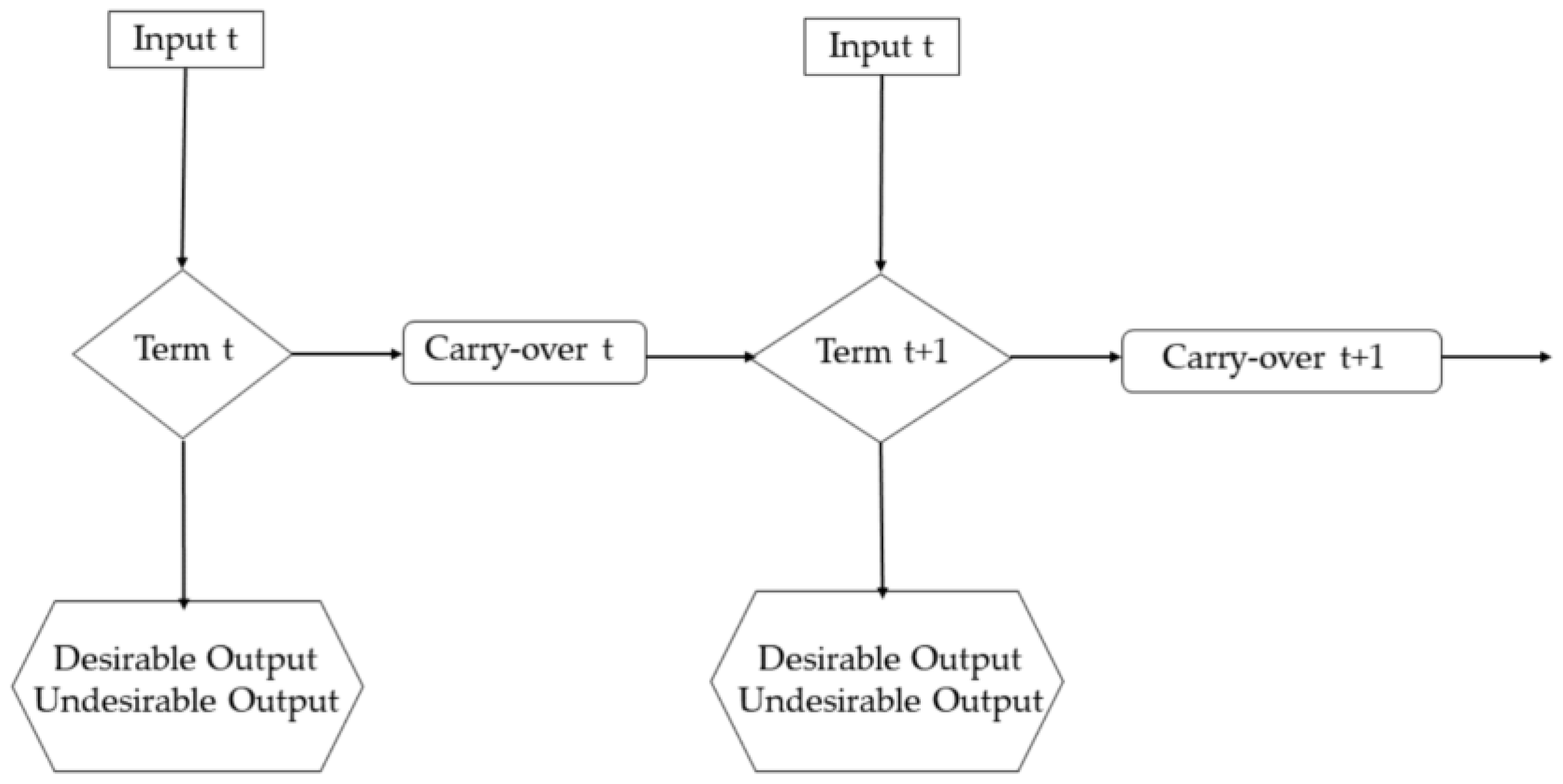
36]. By incorporating green water consumption and carbon emissions in agricultural production into the evaluation indices of AEE, this paper tries to improve the accuracy of AEE estimation and enhance the practical value of the results. The SBM-DEA model used in the existing research on AEE can only conduct a static efficiency analysis, ignoring the long-term effect of specific variables on AEE. As fixed asset investment can be reused in agricultural production, play a continuous role, and be conducive to the cultivation of the technology and talents necessary for long-term agriculture, this paper takes agricultural fixed asset investment as a carry-over variable to construct the dynamic SBM-DEA model of AEE evaluation. This study tries to offer a reasonable model of AEE evaluation, and find some reliable basis for improvements in AEE, coordinated development among regions, and the enhancement of food security in China. The aims include: (1) to establish a novel undesired dynamic SBM-DEA model to evaluate the AEE, taking green water consumption, carbon emissions, and the persistent role of fixed asset investment into consideration; (2) to evaluate the AEE in China and reveal the production efficiency, incorporating both resource consumption and environmental impact; and (3) to unearth the spatiotemporal differentiation of both the AEE and its factor efficiency index, to recognize the provinces that urgently need to improve the AEE as well as the targeted approach.
The rest of this paper is structured as follows:
Section 3 establishes the methods and data source;
Section 4 shows the evaluation results and the spatiotemporal variation in both the AEE and its factor efficiency indices;
Section 5 discusses the results and their policy implications; and, finally, conclusions are proposed in
Section 6.
4. Result Analysis
According to the undesired dynamic SBM-DEA model and data availability, this study used the Max DEA-solver software to calculate the AEE of 31 provinces in China from 2007 to 2018, as well as their agricultural resource-saving potential, agricultural pollution reduction space, and the accumulation effect of carry-over variables, as determined by each slack variable. It also analyzed the spatiotemporal discrepancy of both AEE and the efficiency indices of resource consumption, pollution emission, and fixed asset investment. The study period does not include the years after 2019, mainly to exclude the impact of the COVID-19 epidemic on the labor force, land, machinery, chemical fertilizer, and fixed asset investment in terms of agricultural production. The lack of yield data for other grains and flax in each province in 2019 would not only impact the estimation accuracy for green and blue water input but also affect the consistency of the statistical caliber in the evaluation model. Therefore, 2018 was the end of this study period.
4.1. Spatiotemporal Differentiation Pattern of Agricultural Eco-Efficiency
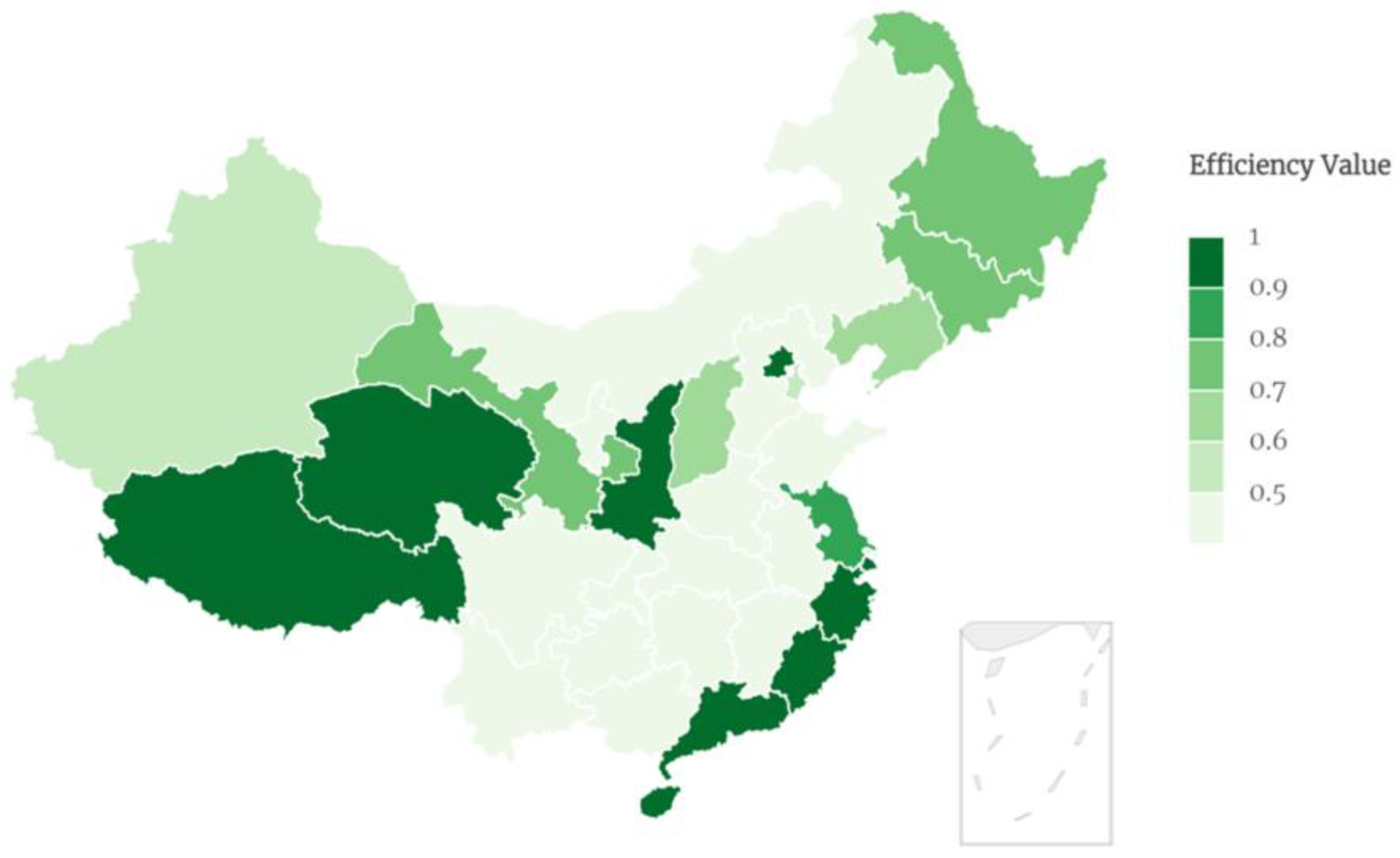
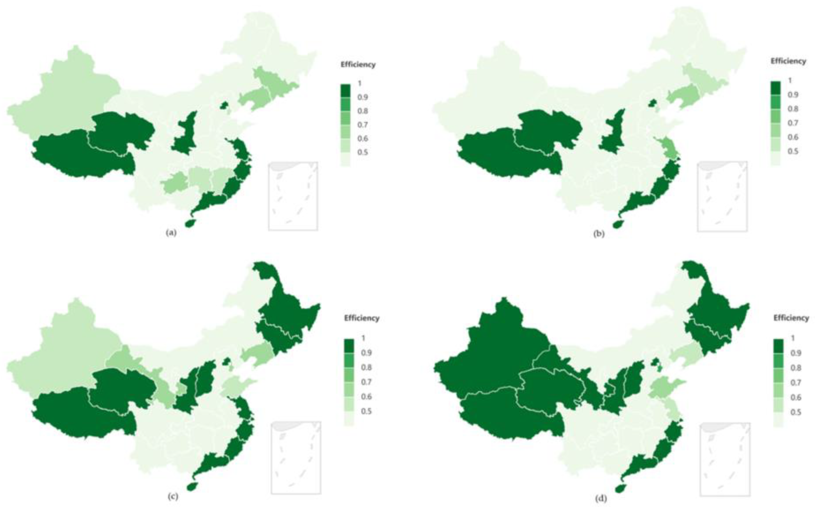
According to the estimation results of the model, the average overall AEE value in 31 provinces of China from 2007 to 2018 was 0.66, and the national average value fluctuated from 0.64 in 2007 to 0.70 in 2018, with an average annual increase of 1%. In the transformation of China’s agricultural green production, the utilization level of agricultural production factors continues to elevate. The AEE in Shanxi, Shandong, Heilongjiang, and Tianjin showed a continuous upward trend over 12 years, and the corresponding growth rate in Shanxi was the largest, followed by that in Shandong. This was attributed to agricultural production structure adjustments and improvements in agricultural production technology in these areas. The efficiency in Jilin, Xinjiang, Gansu, and Ningxia fluctuated with a short-term decline but an overall increase. AEE in Jiangsu, Liaoning, Guizhou, and Hunan showed a downward trend. The AEE of Jiangsu violently altered, fluctuating to some degree in 2010, 2011, 2013, 2014, and 2018, and remaining at 1 in every other year, with the AEE in 2018 measured as 0.60, the lowest of the 12 years. The efficiency in Hunan continued to decrease, from 0.65 in 2007 to 0.53 in 2018, with an annual decline of 1.77%. The efficiency in Guizhou rose to 1 in 2008 and fell in the following years, while that in Yunnan, Sichuan, Hebei, Henan, and Inner Mongolia first declined and then rose after 2015. Jiangxi, Chongqing, and Anhui showed slightly fluctuating efficiencies, which remained stable overall. All the AEE values in other provinces remained at 1.
The calculation results for the average AEE in 31 provinces in China from 2007 to 2018 are shown in
Figure 2, with the value at four time points being presented in
Figure 3. Ranking AEE from high to low, all the provinces can be divided into four groups. Group 1 includes Beijing, Shanghai, Hainan, Qinghai, Shaanxi, Guangdong, Fujian, Tibet, and Zhejiang, whose AEE remained at 1. Jiangsu, Jilin, Heilongjiang, and Gansu form group 2, where the efficiency ranged between 0.72 and 0.87. Group 3 refers to Shanxi, Liaoning, Tianjin, and Xinjiang, with an efficiency between 0.58 and 0.68. Group 4 includes the remaining 14 provinces, whose average annual AEE ranged from 0.33 to 0.49. Therefore, provinces with a high AEE were found to be concentrated in the eastern coastal areas, Jilin and Heilongjiang in the central areas, and several western provinces such as Qinghai, Shaanxi, Tibet, and Gansu. Beijing, Fujian, some other eastern coastal provinces, as well as Qinghai, Shaanxi, and Tibet in the west, presented continuously high levels of AEE during 2007–2018. The provinces with a low AEE were located in central and western China (according to the regional division by the National Bureau of Statistics of China, eastern China consists of Beijing, Tianjin, Hebei, Liaoning, Shanghai, Jiangsu, Zhejiang, Fujian, Shandong, Guangdong, and Hainan; the central region includes Shanxi, Jilin, Heilongjiang, Anhui, Jiangxi, Henan, Hubei, and Hunan; and the western region comprises Inner Mongolia, Guangxi, Chongqing, Sichuan, Guizhou, Yunnan, Tibet, Shaanxi, Gansu, Qinghai, Ningxia, and Xinjiang).
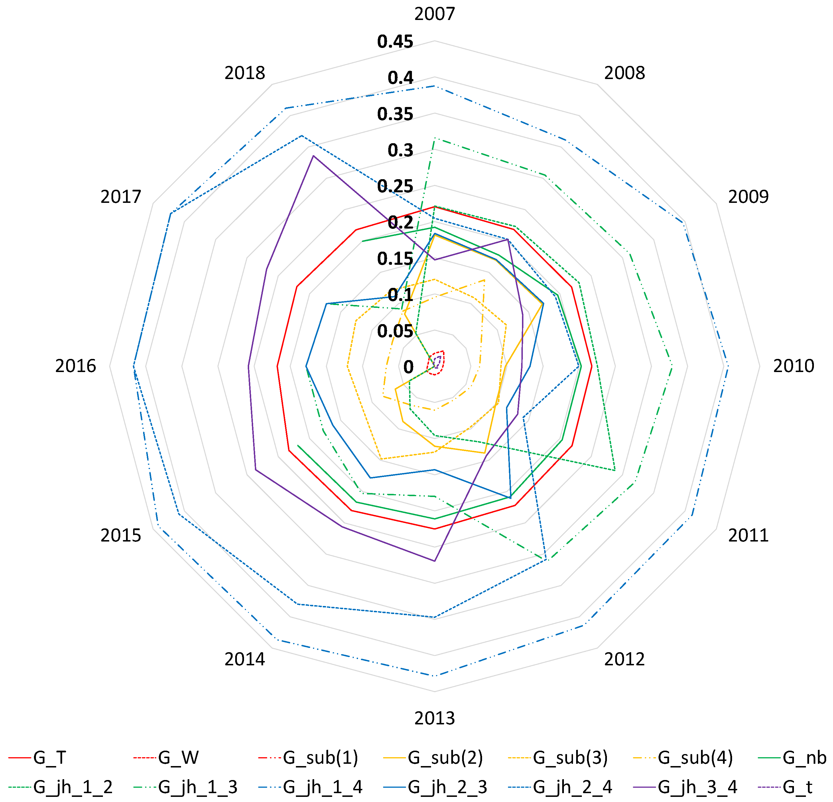
According to the division of the 4 groups of provinces shown above, the Dagum–Gini coefficient decomposition of AEE from 2007 to 2018 was carried out (
Figure 4). The overall spatial difference regarding AEE increased from 2007 to 2015. In 2016, it sharply dropped below the level of 2007 and then fluctuated at this level. The overall spatial discrepancy was mainly derived from inter-group variations, with an annual average contribution rate of 91.10%. The gap between groups 1 and 4 remained large during 2007–2018, and the Gini coefficient between them was always higher than that between any other two groups. The inter-group gap was mainly noted between groups 1 and 3 before 2012, and after 2013, the difference between groups 2 and 4 became one of the main contributing factors to the overall spatial difference. Therefore, when promoting AEE and its overall synergy in China, it is necessary to strengthen the exchanges and cooperation between regions with high and low efficiency, especially collaborations between the groups with the lowest and highest AEE.
4.2. Temporal Evolution of Factor Efficiency Index
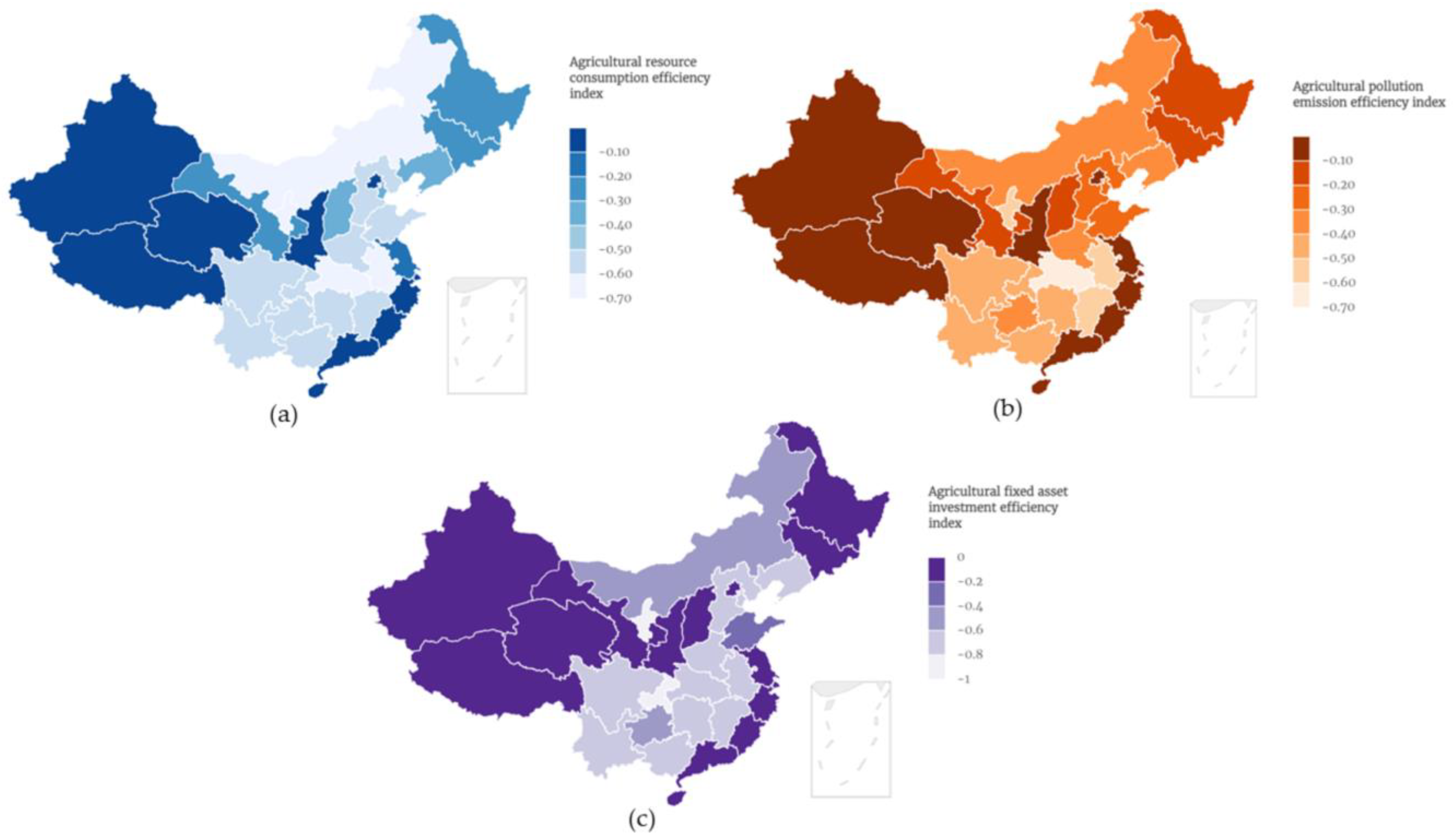
The factor efficiency indices were calculated in this study; then the causes and space for improvements in AEE were analyzed. According to the estimation results, the efficiency indices of agricultural resource consumption, pollution emission, and fixed asset investment in China are shown in
Figure 5.
From 2007 to 2018, the three-factor efficiency indices in 31 provinces were mostly negative, and some were 0, indicating that there was a certain degree of redundancy in the input and output elements as well as in the carry-over variables. The average value of the agricultural resource consumption efficiency index was −0.33, in which the mean efficiency indices of land and blue water input were lower than those of other factors. The average agricultural pollution emission efficiency index was −0.25, where the average efficiency index of agricultural carbon emissions was lower than that for agricultural nitrogen and phosphorus loss. The mean value of the agricultural fixed asset investment efficiency index was −0.36. Therefore, in the three factor efficiency indices, the actual value of agricultural pollution emissions in China was closest to the projection value, and agricultural fixed asset investment showed the most room for improvement.
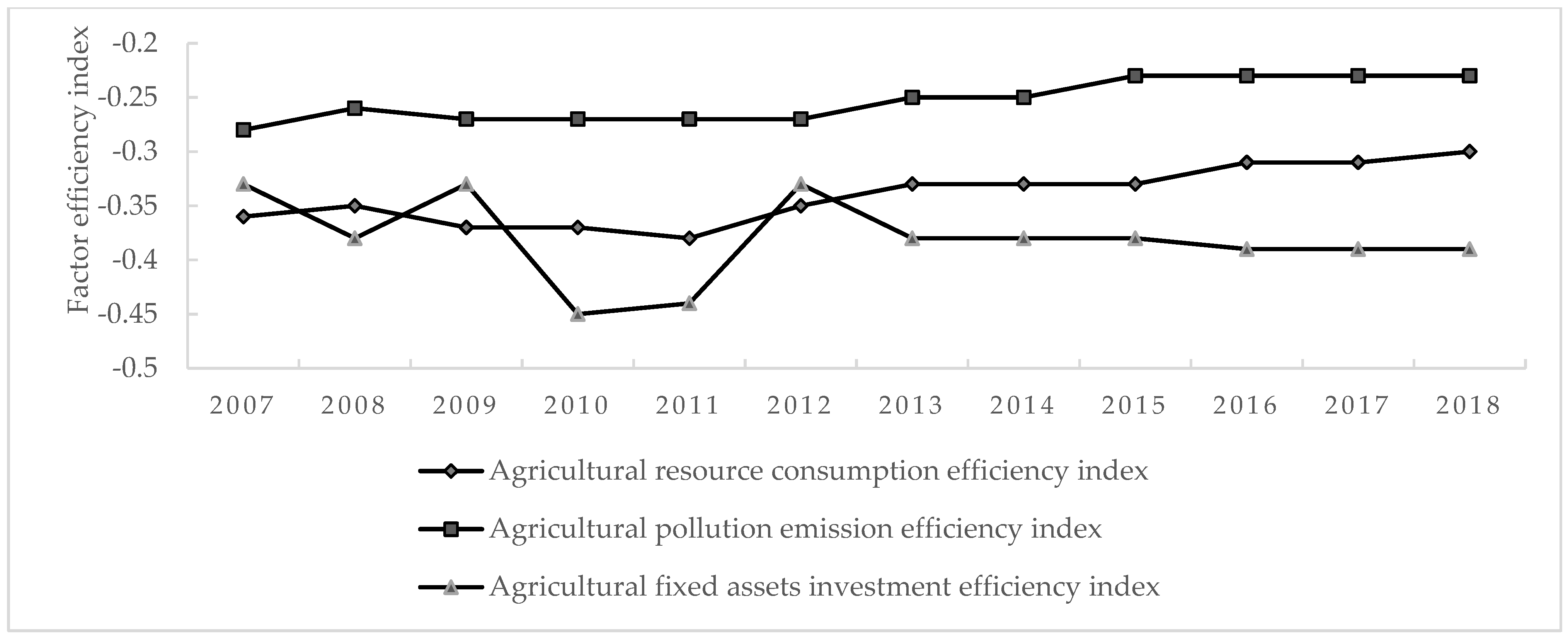
The temporal trends in the factor efficiency indices in China are shown in
Figure 6. The annual average efficiency indices of agricultural resource consumption and pollution emission in 31 provinces rose, whereas the instability of the agricultural fixed asset investment efficiency index was more obvious, showing an overall downward trend. The average annual value of the agricultural resource consumption efficiency index in 31 provinces in 2018 was −0.30, increasing by 1% from 2007. The average emission reduction space of 31 provinces showed a slow downward trend from 2007 to 2018, which reflected the good results achieved regarding reductions in China’s agricultural production emissions. All the factor efficiency indices of agricultural carbon emissions and chemical fertilizer nitrogen and phosphorus loss decreased. The annual mean value of the agricultural fixed asset investment efficiency index in 31 provinces fluctuated, ranging from −0.45 to −0.33 in the last 12 years.
The trend of the agricultural resource consumption efficiency index in half of the 31 provinces from 2007 to 2018 was relatively stable. Provinces with a wavy increase in this index included Shanxi, Inner Mongolia, Shandong, Gansu, Heilongjiang, Xinjiang, and Jilin. In Shanxi, Gansu, and Heilongjiang, this index rapidly increased, reaching −0.69, −0.57, and −0.51, respectively, in 2007. Tianjin’s agricultural resource consumption efficiency index rose steadily in the past 12 years, from −0.47 in 2007 to −0.20 in 2018, with an average annual increase of 6.8%. This index declined in Jiangsu, Guizhou, Liaoning, Hunan, Hubei, Sichuan, Guangxi, Yunnan, Chongqing, Hebei, Henan, and Anhui. The fluctuations seen in Jiangsu were the most obvious, with the index plunging in 2011, 2014, and 2018, reaching a minimum of −0.40 in 2018, which is consistent with the severe fluctuations of AEE. The agricultural resource consumption efficiency index in Hunan and Hubei showed a steady decline, with the former showing a more stable decline, from −0.48 in 2007 to −0.59 in 2018, with an annual average decline of 1.9%.
The agricultural pollution emission efficiency index in Shanxi, Tianjin, Heilongjiang, Shandong, Jilin, Gansu, and Xinjiang surged, with fluctuations from 2007 to 2018. The index in Tianjin showed the largest growth; it was lower than −0.40 in 2007 and, after two short declines, achieved a maximum of 0 in 2018. In Jiangsu, Guizhou, Hunan, Liaoning, Yunnan, Guangxi, Henan, Chongqing, Ningxia, Hubei, and Sichuan, the agricultural pollution emission efficiency index showed a wavelike decrease. In other provinces, this index was stable, with no obvious change.
In most provinces, the agricultural fixed asset investment efficiency index showed a fluctuating downward trend and finally stabilized in the range from −0.92 to −0.77. In Liaoning, Xinjiang, Heilongjiang, Shanxi, Jilin, and Shandong, this efficiency index declined to a certain extent in the early stage and finally showed an increasing trend. In Xinjiang, Heilongjiang, Shanxi, and Jilin, the index eventually increased to the maximum value of 0; in Liaoning, the index increased from −0.55 in 2007 to −0.23 in 2018, and in Shandong, it rose from −0.36 in 2007 to −0.1 in 2018, with an annual average increase of 0.46% and 0.52%, respectively.
4.3. Spatial Differentiation of Agricultural Resource Consumption Efficiency Index
The standard deviation of the agricultural resource consumption efficiency index of 31 provinces in China showed an increasing annual trend, from 0.29 in 2007 to 0.31 in 2018, indicating an expanding spatial difference (
Table 2). According to the division of the four groups of provinces by the AEE value shown above, the Dagum–Gini coefficient decomposition of the agricultural resource consumption efficiency index from 2007 to 2018 was created. The results show that the spatial difference in the agricultural resource consumption efficiency index mostly stems from the inter-group disparity, with a contribution rate of up to 93.86%. The Gini coefficient between group 1, with an AEE of 1, and other groups is far higher than that of any other two groups. Therefore, an effective way to reduce the degree of spatial non-equilibrium in the utilization of agricultural resources would be to strengthen the sharing of agricultural technology and management between provinces in group 1 and others.
The annual average value of the provincial agricultural resource consumption efficiency index in Beijing, Fujian, Guangdong, Hainan, Qinghai, Shaanxi, Shanghai, Tibet, and Zhejiang was 0, which was consistent with their high AEE. Provinces with a low agricultural resource consumption efficiency index were Ningxia, Anhui, Inner Mongolia, Hubei, Henan, and Guangxi, with a value lower than −0.60. Ningxia had the largest room for improvement in the efficiency of irrigation blue water input, where the blue water input efficiency index was −0.90, while the efficiency indices of land and machinery input were both −0.78. Anhui’s agricultural resources that must urgently be saved are similar to those in Ningxia. The efficiency indices of land, blue water, and machinery input in Anhui were lower than −0.7. Meanwhile, the blue water input in Hebei and Henan was also far higher than the target amount, with low utilization efficiency in farmland irrigation. The land input efficiency index in Inner Mongolia was −0.81, the lowest of all the kinds of agricultural resource consumption efficiency indices. The labor input efficiency index in Guangxi was lower than −0.70, which was the main contributor to its low agricultural resource consumption efficiency index.
4.4. Spatial Differentiation of Agricultural Pollution Emission Efficiency Index
The standard deviation of the agricultural pollution emission efficiency index of 31 provinces in China during 2007–2018 was relatively stable, fluctuating slightly at 0.25 with a steady spatial difference (
Table 3). When groups were divided according to the AEE value given above, the Dagum–Gini coefficient decomposition of the agricultural pollution emission efficiency index was also calculated. A total of 87.40% of the spatial difference in this index was derived from inter-group disparity, especially the variation between the group with an AEE of 1 and other groups. This is similar to the results for the composition of spatial imbalances in the agricultural resource consumption efficiency index.
The annual average value of the agricultural pollution emission efficiency index in Xinjiang, Beijing, Fujian, Guangdong, Hainan, Qinghai, Shaanxi, Shanghai, Tibet, and Zhejiang was 0, coinciding with their high AEE. The reduction space for agricultural pollution emissions in Jiangsu, Jilin, Gansu, and Heilongjiang was between 10% and 20%. The nitrogen and phosphorous loss efficiency index in Jilin and Heilongjiang was 0, and that in Gansu was also close to 0, but the carbon emission reduction space of the 3 provinces was as high as 30% or more. The lowest agricultural pollution emission efficiency index was seen in Hubei, Anhui, Ningxia, and Jiangxi, at below −0.50. The reduction space for nitrogen and phosphorus loss in these four provinces was about twice as much as the national level. The reduction potential for carbon emissions in Ningxia was also twice as high as the national average, and that space in Hubei was 3.45 times the national level.
4.5. Spatial Differentiation of Agricultural Fixed Asset Investment Efficiency Index
The standard deviation of the agricultural fixed asset investment efficiency index of 31 provinces in China increased from 0.22 in 2007 to 0.42 in 2018, and the dispersion of the data increased each year, showing an obvious expansion trend of spatial divergence. Consistent with the analysis of spatial differentiation in the other two efficiency indices, the Dagum–Gini coefficient decomposition of the agricultural fixed asset investment efficiency index from 2007 to 2018 shows that inter-group differences are the most important source of the overall spatial non-equilibrium in the agricultural resource consumption efficiency index, with a contribution rate of 87.21%. The Gini coefficient between the high-AEE group and other groups is the highest between any two groups.
Comparing the annual average value of the agricultural fixed asset investment efficiency index in each province in
Table 4, provinces with an index value of 0 included Beijing, Fujian, Guangdong, Hainan, Qinghai, Shaanxi, Shanghai, Tibet, Zhejiang, and Xinjiang, which was consistent with their high AEE. In Jiangsu, Gansu, Heilongjiang, Jilin, Shaanxi, and Shandong, the room for improvement was within 25%, demonstrating that the fixed assets were well utilized there. In contrast, the agricultural fixed assets investment efficiency index in 10 provinces, such as Ningxia, Chongqing, Hebei, Jiangxi, Tianjin, Sichuan, Yunnan, Guangxi, Hubei, and Henan, was the lowest, and their corresponding redundancy exceeded 70%; the redundancy in Ningxia and Chongqing was more than 80%. This redundant index indicated that the matching degree between fixed asset investment and other agricultural production factors could be improved.
A cluster analysis of the annual average factor efficiency indices by provinces was undertaken, the Euclidean distance was calculated, and classification was carried out according to the average distance. The results are shown in
Table 5. Provinces such as Beijing, Fujian, and Guangdong in cluster 1 had high results for each index, while each index in Jilin, Heilongjiang, Gansu, and Shanxi in cluster 2 was moderately high. The efficiency indices of agricultural resource consumption and pollution emission in Liaoning and Tianjin in cluster 3, and the efficiency indices for agricultural pollution emission and fixed asset investment in Guizhou and Shandong in cluster 4 were moderately low, and all the other indices in the 2 clusters were low. All 3 indices in provinces in cluster 5 were low, consistent with the results of the spatial differentiation analysis shown above.
5. Discussion
5.1. Discussion of the Correlation between Input and Output Indicators
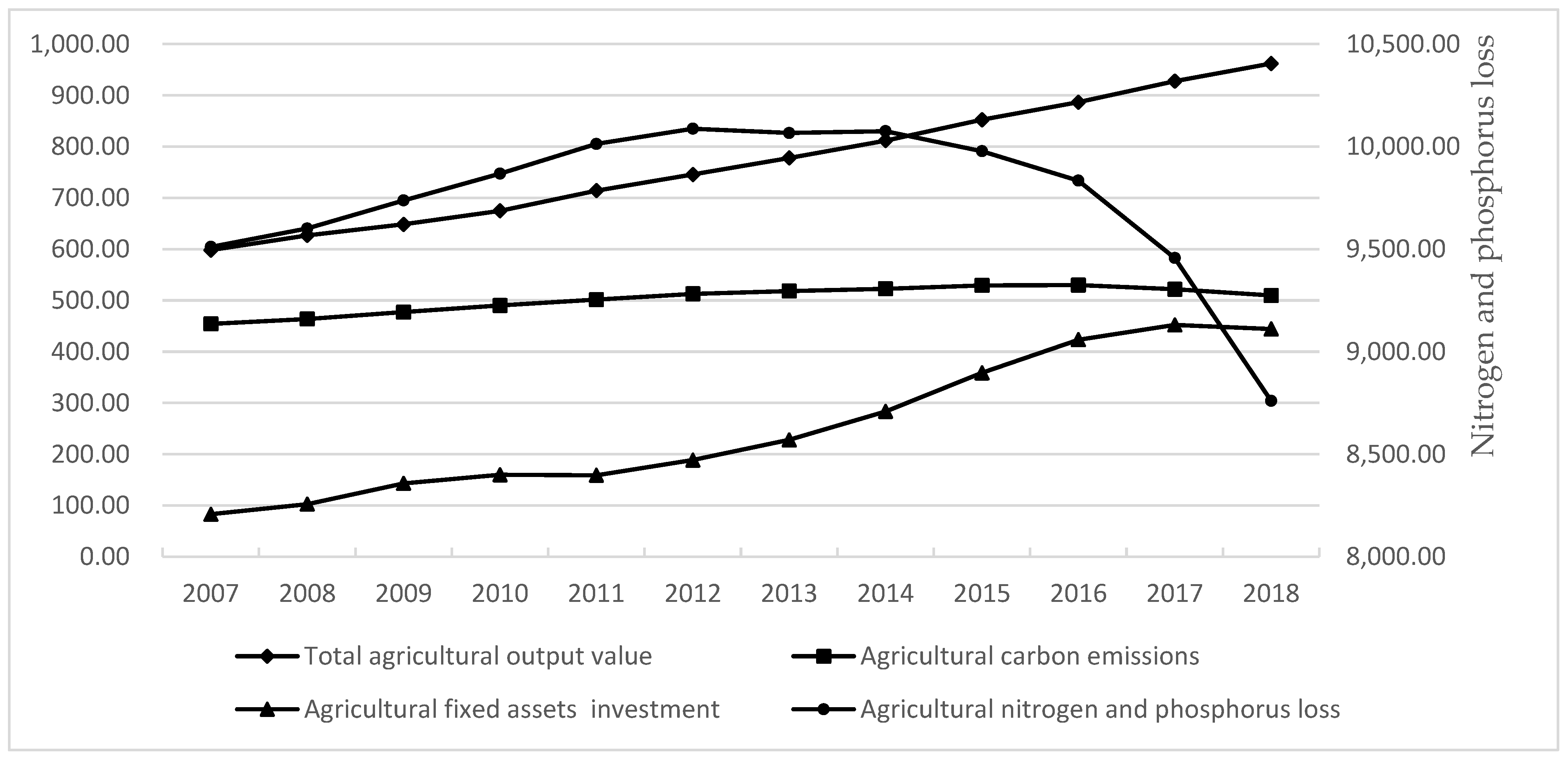
The trends in the annual average AEE input and output indicators in China are depicted in
Figure 7.
Over 12 years, the agricultural fixed asset investment and the total agricultural output value showed an obvious upward trend, and carbon emissions remained stable. However, the loss of nitrogen and phosphorus due to the application of fertilizers declined. A series of agricultural non-point source pollution-control actions achieved some good effects, such as “the activity of China’s agricultural non-point source pollution prevention and control”, “National Agricultural Sustainable Development Plan (2015–2030)”, and the “Zero Growth Programme of Action for Fertilizer Use by 2020”.
Table 6 shows the correlation coefficient between input and output indicators in the AEE evaluation in China.
The green water input is closely correlated with either the total agricultural output value or the agricultural carbon emissions, with the two correlation coefficients reaching as high as 0.92. It is also highly and positively correlated with losses in agricultural nitrogen and phosphorus, where the correlation coefficient was 0.76. All these correlation coefficients are much higher than the ones between blue water input and these three output indicators. This is consistent with the dependence of crop growth on green water and verifies that the use of green water cannot be ignored in the calculation of AEE. The correlation coefficients between chemical fertilizer input and these three output indicators were all above 0.8. The correlation coefficient between chemical fertilizer input and either total agricultural output value or carbon emissions was almost 0.92, respectively. These reflect not only the effect of fertilizer input on improvements in agricultural output value in China but also the important role of fertilizer application in agricultural carbon emissions. Among all the input indicators, the agricultural labor force input showed the weakest correlation with the three output indicators, with correlation coefficients below 0.5. It can be inferred that, with the continuous rise in labor costs, the degree of mechanization of agricultural production in China accelerated and the relationship between labor force input and agricultural output gradually declined. Finally, the correlation coefficients between the agricultural fixed asset investment and the three output indicators are relatively high. There is still a certain correlation between the agricultural fixed asset investment in the current year and the output indicators in the subsequent years. This also proves the opinion of this study: agricultural fixed asset investment has a continuous effect on agriculture production, and it is rational to set this as a carryover variable.
5.2. Discussion of the Agricultural Eco-Efficiency
As the calculation results show, the annual average value of AEE in China increased from 2007 to 2018. This is consistent with the results of Yang et al. [
27], Wu et al. [
48], and Cheng et al. [
49]. It can be proved that national strategies such as new rural construction, rural revitalization, ecological civilization construction, and green development in China have made certain progress toward promoting the sustainable development of the agricultural economy. Continuing and strengthening this trend would be significant for food security in China, which faces the challenges of a large population, increased demand, and tight constraints on resources and the environment. It is also consistent with the point that national policy incentives have become indicators of the Chinese AEE’s evolution [
50].
Moreover, the AEE value in this study is smaller than the results of Yang et al. [
27], Wu et al. [
48], and Cheng et al. [
49]. The average AEE of China in 2018 was 0.78 in the work of Yang et al. [
27] and higher than 0.9 in the work of Wu et al. [
48], while it was 0.7 in this study. This is primarily because this study additionally considers both the green water input and agricultural nitrogen and phosphorus loss, and the increase in both input and undesirable output directly diminished the level of AEE. Meanwhile, the persistent role of fixed asset investment in agriculture production was integrated into the AEE evaluation method in this study, whereas it was not in the previous research. The results of this study show that the value of the agricultural fixed asset investment efficiency index is smaller than that of either the resource consumption efficiency index or pollution emission efficiency index. This low fixed asset investment efficiency index also makes the AEE lower than the AEE obtained without considering this index.
Yang et al. concluded that the growth rate of AEE in major grain-producing areas is lower than that in other regions of China, which coincides with the results of this study [
27]. This is closely relevant to the decrease in the agricultural resource consumption efficiency index in Jiangsu, Guizhou, Liaoning, Hebei, Hunan, and Hubei; the decline that occurs with fluctuations in the agricultural pollution emission efficiency index in Yunnan, Guizhou, and Jiangsu; and the decreasing volatility of the agricultural fixed asset investment efficiency index in the major grain-producing areas except for Heilongjiang, Jilin, Liaoning, and Shandong. This shows the urgency of further improving resource utilization efficiency and controlling non-point source pollution and carbon emissions in major grain-producing areas.
In the analysis of spatial differences, we found that the inter-provincial gap in AEE gradually widened from 2007 to 2015 and decreased after 2016. These results are consistent with those of Cheng et al. [
49], demonstrating the remarkable achievement of ecological civilization construction in China.
This study shows that the AEE of some provinces in central and western China, which remained low throughout the declining trend in the study period, is also consistent with the results of Cheng et al. [
49]. The studies of Wu et al. [
48], Cheng et al. [
49], and Chen et al. [
51] showed that, in the eastern, central, and western regions of China, the eastern region showed the highest AEE and the central region showed the lowest, consistent with the results of this study. Beijing, Shanghai, Hainan, and some other provinces presented a higher AEE related to the more widespread utilization of agricultural fixed asset investments and lower agricultural pollution emissions. This coincides with their high priority for the protection of the agricultural ecological environment. Provinces such as Zhejiang and Jiangsu have actively developed modern and intensive ecological agriculture and accumulated certain technology and experience regarding reductions in agricultural carbon emissions and nonpoint source pollution treatment. Accordingly, their AEE level was at the forefront of the country. Guangdong, Fujian, and Tianjin are pioneering areas of social and economic development in China. They have a good foundation of capital and technology in the development of eco-agriculture and have scale advantages in the agricultural labor force, machinery investment, and chemical fertilizer applications. Liaoning, one of the major grain-producing areas in China, has excellent agricultural conditions, such as land and climate. These can vigorously reform agricultural science and technology and have advantages regarding human reserves and mechanical transformation. Accordingly, the level of agricultural output was high, leading to a high AEE value. Tibet, Qinghai, Shaanxi, Gansu, Xinjiang, and other northwest provinces maintained a high AEE mainly due to their relatively higher utilization efficiency of land, water, and other resources and lower agricultural pollution emissions. Among the 31 provinces, the efficiency indices of agricultural resource consumption, pollution emissions, and fixed asset investment in some provinces of the central region, such as Inner Mongolia, Hubei, Anhui, and Ningxia, were in the backward position, resulting in their having a low AEE.
The analysis of spatial difference patterns in AEE can directly show the efficiency level of each province and help distinguish the urgency of efficiency improvements in different regions. However, a spatial variation analysis only shows the results of regional comparisons, which need to be combined with the in-depth development conditions, the current situation, and the characteristics of the region to help find the reasons for this high or low regional efficiency and provide a practical basis for the targeted suggestions. Therefore, on the basis of the inter-provincial comparison of AEE, the specific efficiency index level of the input and output indicators, and the actual development, the implementation of national policies and the local policy orientation, the reasons for the AEE level of each province can be determined, and local countermeasures are put forward to improve this.
5.3. Discussion of the Factor Efficiency Index
From the temporal evolution of the AEE factor efficiency index, China made some achievements in agricultural resource conservation and emission reduction, especially regarding the control of chemical fertilizer input. The chemical fertilizer input efficiency index increased greatly, significantly contributing to the increase in agricultural resource consumption efficiency. In recent years, the government has issued a number of binding regulations for agricultural pollutant emissions. Although negative, the agricultural pollution emission efficiency index was still slowly rising, showing some progress in agricultural pollution control.
This study holds that the relationship between agricultural fixed asset investment and AEE is not a simple linear relationship and is affected by the cooperation of other factors during the process of agricultural production. This paper argues that the redundancy of agricultural fixed asset investment calculated by the model is not the absolute redundancy of the investment scale. The matching degree between agricultural fixed asset investment and other input factors in production also results in the low utilization efficiency of agricultural fixed asset investment.
The efficiency indices of blue water, land, and machinery input were low in Ningxia. Problems such as the fragmentation of water resources management, mismatches between agricultural water price, water scarcity, and ecological environment costs lead to the low utilization efficiency of local irrigation water. The lower agricultural land input efficiency index in Ningxia was related to the unsmooth circulation of local agricultural land and the extensive land use and utilization behavior in some areas. Finally, while Ningxia was rapidly improving the level of agricultural machinery and equipment, the utilization efficiency of the machinery resources was still relatively insufficient. The agricultural water consumption in either Anhui, Hubei, or Henan, the 3 major grain-production provinces, exceeded 15 billion cubic meters in 2019. Combined with the low blue water input efficiency index in these three provinces, raising the utilization efficiency of irrigation water is an important way to improve their AEE. Inner Mongolia has a vast territory, and its per-capita arable land area ranks first in the country. However, the basic conditions of its land resources are poor. In addition, the local land productivity is relatively low and unstable, and the proportion of high-yield fields is small. Therefore, the low land input factor efficiency index is an important contributor to its low AEE. As a region with relatively lagging economic development, Guangxi has a serious problem with aging agricultural employees. The redundancy of labor input is relatively prominent, leading to its relatively low AEE.
The local agricultural output was relatively large in Hubei and Anhui, but the efficiency index of either nitrogen and phosphorus loss or carbon emissions was low. The reduction space of agricultural carbon emissions in Ningxia was large, and the factor efficiency index showed that actual agricultural carbon emissions in the region exceeded 65% of the optimal target value. Located northwest inland, Ningxia is an important animal husbandry and planting base in China. However, high carbon emission intensity poses a threat to the local ecological balance. Reducing agricultural greenhouse gas emissions has become the focus of green agricultural development in Ningxia. According to the results of the nitrogen and phosphorus loss efficiency index, the actual nitrogen and phosphorus loss exceeded 57% of the optimal target value in Jiangxi, a traditional agricultural province in China. In the last 10 years, the average amount of cultivated land in Jiangxi was 45.84 kg/hm2, which was higher than the national average. The application of chemical fertilizers can temporarily supplement soil minerals and increase farmland yields. However, the excess chemical fertilizers that are not absorbed by crops can cause pollution and become an unfavorable factor restricting agricultural development.
The redundancy of agricultural fixed asset investment in 10 provinces, such as Ningxia, Chongqing, and Hebei, was more than 70%, indicating that the promotion effect of the local fixed asset investment on AEE was not fully utilized. In recent years, China’s agricultural production technology and infrastructure were continuously enhanced, and the total investment in agricultural fixed assets and the number of projects showed a rapid upward trend. However, the economic benefits of agricultural fixed assets investment gradually diminished. This may be due to the following two aspects. First, there are spatial differences at the level of either agricultural economic development or agricultural fixed asset investment, and the investment scale is also uneven among provinces. The extensive management of agricultural fixed asset investment in most regions is not conducive to improving investment utilization efficiency. Therefore, each province should adjust the investment structure of fixed assets according to their local agricultural production. Guangxi, Yunnan, and other regions with a larger population but less arable land, extensive land management, and a seriously aging labor force require the urgent application of agricultural machinery and equipment. Sichuan, Jiangxi, and other provinces with fragile agricultural foundations have higher requirements for agricultural water conservancy infrastructure. Second, the low level of technological transformation investment in agricultural investment is particularly prominent in China. Some outstanding technological transformation projects face difficulties in obtaining timely funding and cannot be transformed into real productivity, which is not conducive to the improvements in independent agricultural innovation and restricts the multiplier and leverage effect of investment on driving agricultural development.
5.4. Policy Implications
To boost ecological agriculture and the green economy and advance coordinated and sustainable development, either between the agricultural economy and the environment or amongst regions, the following suggestions are put forward based on the calculation results for AEE in China and the pattern of spatiotemporal differentiation:
(1) Interregional cooperation should be augmented to enhance the overall AEE and facilitate interregional coordination in China. In the results, the gap between provinces with a high AEE and those with a low AEE is the main contributor to the overall spatial imbalance in either the AEE or factor efficiency indices in China, with a contribution rate of above 85%. Moreover, the spatial difference between the agricultural resource consumption efficiency index and that of the agricultural fixed asset investment efficiency index expanded during 2007–2018. Thus, the AEE in provinces has certain solidification characteristics, and the provincial disparity of both the agricultural resource utility level and the fixed asset use efficiency increased. To improve AEE and mitigate the spatial non-equilibrium, we should focus on strengthening the exchanges and associations between high-AEE provinces such as Beijing, Shanghai, and Hainan and low-AEE provinces such as Guizhou, Jiangxi, and Chongqing, especially regarding resource utilization and fixed asset use;
(2) A differentiated strategy should be implemented to raise regional AEE. Due to the divergence between agricultural production status and economic development level among regions, there are certain differences in the level of AEE and factor efficiency indices in various regions. Therefore, it is necessary to look for shortcomings in regional agricultural development and formulate personalized development strategies to promote AEE. According to the AEE measurement results and factor efficiency indices shown above, the key provinces that need to increase their AEE are listed in
Table 7.
For the key provinces that need to accelerate AEE, the critical points to be improved are listed in
Table 8, in line with the efficiency index. Suppose a factor efficiency index in a province ranks 25th or lower among the 31 provinces. In that case, the utilization level of this factor or the level of undesirable output emissions is considered to be significantly lower than that of other provinces, and it is strongly necessary for the province to improve the utilization efficiency or control the undesirable output. Suppose the provincial ranking of the efficiency index is lower than its AEE ranking in 31 provinces and the gap is greater than or equal to 5 places. In that case, it is believed that the utilization of this factor greatly affects the AEE level of the province, and it is moderately necessary for the province to improve the use efficiency of this factor or control the intensity of undesirable outputs. Suppose the ranking of a factor efficiency index in a province is lower than its AEE ranking and the gap is within 5 places. In that case, it is suggested that the province further improves the utilization efficiency of the factor or the intensity of the undesired output to improve the AEE.
For Beijing, Shanghai, Hainan, and other provinces with a high AEE, it is necessary to further develop modern ecological agriculture under relatively perfect agricultural infrastructure and development conditions, make full use of modern scientific and technological achievements and modern management, learn from effective traditional agriculture, and improve the economic, ecological, and social benefits of agriculture. Henan, Inner Mongolia, Hubei, Anhui, Ningxia, and other provinces with relatively low AEE all show a great need to improve the utilization efficiency of chemical fertilizer. They should strengthen the policies and technical guidance for fertilizer application based on the actual local planting structure and conditions and integrate a technological model of fertilizer reduction and efficiency increases. New products, such as high-efficiency and slow-release fertilizers and biofertilizers, should be developed; advanced and applicable fertilization machinery should be promoted; and socialized service organizations should be cultivated to provide unified distribution and control services. Anhui shows a strong need to improve the utilization efficiency of labor, land, blue water, green water, machinery, etc., as well as to reduce the intensity of nitrogen and phosphorus losses. It is necessary for this province to strengthen the concept of green development, accelerate the development of intensive ecological agriculture, and pay attention to cultivated land and three-dimensional cultivation. To improve its AEE, Anhui also should improve the quality of workers and introduce technical assistance, strengthen facility agriculture and standardized management, and reinforce the agricultural infrastructure and ecological environment construction;
(3) The redundancy of agricultural production inputs should be reduced. In Ningxia, Anhui, Inner Mongolia, Hubei, Guangxi, Henan, and other provinces with a low agricultural resource consumption efficiency index, improvements in resource allocation and a reasonable standard system of the agricultural ecological environment should be formulated according to the current local situation of agricultural production and natural conditions, such as water-source reserves and soil fertility, to improve the utilization efficiency of agricultural land and water resources, especially irrigation blue water, and avoid large redundancies of input factors. Balancing the distribution of resources across the country and strengthening the supervision and management of these resources would improve the efficient utilization of these resources in China. Water-saving irrigation, fallow rotation, the integration of planting and raising, and other modern agricultural development models can also be facilitated to develop resource-intensive agriculture;
(4) Agricultural science and technology should be strengthened to reduce agricultural pollution emissions. For regions in which the agricultural pollution emission efficiency index is below −0.50, such as Hubei, Anhui, Ningxia, and Jiangxi, the agricultural science and technology should be improved. The government and other relevant organizations should actively strive to introduce new agricultural machinery and key energy-saving and environmentally friendly technologies to minimize pollution. The previous business model of pursuing economic output should shift to ecological agriculture development using information technology and big data management, which will raise the AEE;
(5) The utilization of agricultural fixed asset investments should be improved. The results show that the current agricultural fixed asset investment faces input redundancy and low comprehensive utilization efficiency. Therefore, in provinces such as Ningxia, Chongqing, and Hebei, where the redundancy of agricultural fixed asset investment exceeds 70%, government agencies need to further furnish investment mechanisms to support agriculture and reduce the redundancy of agricultural fixed asset investments by optimizing the investment structure and strengthening related management. These provinces should improve the management of fixed assets investment so that planning, design, construction, and other departments can work collaboratively and efficiently and prioritize farmland water conservation and the agricultural service system.


