Article

Real-Time Pricing Method for Spot Cloud Services with Non-Stationary Excess Capacity

School of Business, East China University of Science and Technology, Shanghai 200237, China
*
Author to whom correspondence should be addressed.
Sustainability 2023, 15(4), 3363; https://doi.org/10.3390/su15043363
Submission received: 10 October 2022 / Revised: 7 February 2023 / Accepted: 9 February 2023 / Published: 12 February 2023

Abstract

:
Cloud operators face massive unused excess computing capacity with a stochastic non-stationary nature due to time-varying resource utilization with peaks and troughs. Low-priority spot (pre-emptive) cloud services with real-time pricing have been launched by many cloud operators, which allow them to maximize excess capacity revenue while keeping the right to reclaim capacities when resource scarcity occurs. However, real-time spot pricing with the non-stationarity of excess capacity has two challenges: (1) it faces incomplete peak–trough and pattern shifts in excess capacity, and (2) it suffers time and space inefficiency in optimal spot pricing policy, which needs to search over the large space of history-dependent policies in a non-stationary state. Our objective was to develop a real-time pricing method with a spot pricing scheme to maximize expected cumulative revenue under a non-stationary state. We first formulated the real-time spot pricing problem as a non-stationary Markov decision process. We then developed an improved reinforcement learning algorithm to obtain the optimal solution for real-time pricing problems. Our simulation experiments demonstrate that the profitability of the proposed reinforcement learning algorithm outperforms that of existing solutions. Our study provides both efficient optimization algorithms and valuable insights into cloud operators’ excess capacity management practices.

1. Introduction

Operators of cloud services, such as Alibaba Cloud (Alicloud) and Amazon Web Services (AWS), rent out computing capacity (virtual machines, VMs) as a cloud service to millions of users. These users, ranging from individuals to large institutions, usually rent and pay only for a set of VMs through a posted fixed-pricing model with service-level agreements (SLAs). In the fixed-pricing market, some users enter into long-term contracts to reserve resources, and many choose to obtain resources on demand (i.e., pay as you use). The utilization of these resources is highly time-varying, compounded with uncertain peak–trough changes [1]. During trough times, VMs, on average, run under 30% capacity in global data centers [2], with the majority of these running under 20% utilization [3]. Resource utilization can have sudden unexpected peak–trough shifts [4]. For example, the applications deployed on these resources have new product launches and marketing campaigns, which suddenly generate a huge workload influx [5]. This high volatility for time-varying resource utilization leads to non-stationary excess capacities, which are surplus capacities after meeting the usage of fixed-pricing markets. Considering the perishable and non-storable nature of services in the cloud, the unused excess computing capacities are not able to be transferred from one period to the next. Excess capacity will lead to the potential waste of resources, not to mention the fact that cloud operators still need to pay for these excess capacities (e.g., electricity, hardware, and maintenance costs).
Managing non-stationary excess capacity without violating the written SLAs has become a significant emerging issue. Therefore, some leading cloud operators, including AWS and Alicloud, have launched a relatively new type of service: low-priority spot (pre-emptive) services. Taking Alicloud as an example, it adopts a variable price that is adjusted every five minutes with the following statements: “Spot (preemptive) instance is the temporarily unused regular service (e.g., Elastic Compute Cloud instances), and is offered at a lower price than on-demand instances. Every spot user is required to indicate a maximum price that the user is willing to pay. Only users with a willingness to pay higher than the current spot price can get the spot cloud service. However, if the market price varies higher than the user’s bid or if supply and demand change, the instances are automatically released [6]”. Because there is no SLA violation for low-priority spot services, the operators can reclaim capacities and interrupt these spot users’ computing jobs when resource scarcity occurs. Therefore, this special real-time pricing mechanism for spot cloud services can be completely adapted to the non-stationarity of excess capacity.
However, due to the non-stationarity of excess capacity with uncertain peak–trough changes, cloud operators cannot directly observe the excess capacity available to spot services for every given spot price decision in advance; that is, when making price decisions for spot cloud services, operators cannot know the excess capacity that can be provided to spot cloud services during the decision period. To avoid revenue losses from offering sub-optimal prices, operators also need to make spot pricing decisions based on all historical excess capacities, which causes spot pricing decisions to face a huge search space and to be difficult to adapt to real-time decision-making requirements for spot pricing.
Dynamic pricing for cloud computing is an attractive scheme and of great interest to the academic community devoted to seeking the optimal dynamic pricing policy. Ben-Yehuda et al. [7] and George et al. [8] have examined the dynamic pricing traces of spot services from Amazon EC2 and Alibaba Cloud, and provided qualitative changes which showed that spot prices are artificially set. Xu et al. [9] developed and analyzed market-driven dynamic pricing mechanisms for spot instances, and adopted a revenue management framework to formulate the revenue maximization problem with dynamic pricing as a stochastic dynamic program. Furthermore, Alzhouri et al. [10] developed a systematic approach toward the dynamic prices of stagnant VMs of both one class and multiple classes to achieve the maximum expected revenue within a finite discrete time horizon. Lei et al. [11] examined a dynamic pricing problem in the face of non-stationary, stochastic, and price-sensitive demand for instances, proposed heuristic methods, and showed the near optimality of the proposed methods when both demand and supply are sufficiently large. Bonacquisto et al. [12] proposed an alternative, dynamic pricing model for selling unused capacity. It is worth pointing out that these works focused on fixed excess capacity while ignoring the non-stationarity of excess capacity. In fact, an efficient real-time spot pricing method should rely on non-stationary excess capacity supply and interruptible demand sides, and will also need an integrated framework that must be considered.
The research on non-stationarity in cloud environments mainly focuses on improving the prediction accuracy of data center resource utilization [13,14]. However, the high volatility in workload makes it difficult to estimate future resource utilization accurately in real time. Additionally, pricing decisions based on predicted resource utilization can only obtain local optimal policies. The non-stationarity in the cloud environment has different workload patterns partitioned by random peak–trough points [15]. When the peak–trough points are detected, pattern structures before and after these points can be estimated based on historical data. Detecting when these peak–trough points happen in a univariate time series has a long, rich history in the statistical literature. Palshikar [16] measured different peak point detection algorithms in any given time series. Tahir et al. [17] investigated the online burst detection technique using sample entropy. Based on changepoint detection thinking, this paper identifies cloud computing change patterns and learns optimal pricing policies for different patterns.
Reinforcement learning (RL) is a simulation-based method that can autonomously learn effective policies for sequential decision problems under uncertainty [18]. As a simulation-based algorithm, decision makers learn how to make optimal pricing decisions by interacting with stochastic simulated environments. Driven by the advantages of optimal learning under uncertainty, RL has become an important tool for revenue management and dynamic pricing problems. Cheng [19] applied the Q-learning approach to dynamic pricing in e-retailing. Gosavii et al. [20] adopted the RL technique to a single-leg airline revenue management problem with multiple fare classes and overbooking. Zhang et al. [21] applied the Q-learning approach to real-time pricing in a smart grid to solve the MDP model without the acquisition of transition probabilities. Alsarhan et al. [22] integrated computing resource adaptation with service admission control based on an RL model. These studies on the application of an RL methodology in revenue management all assume that the environment model is stationary.
The stationarity assumption of the sequential decision problems greatly simplifies real complex environments. Therefore, recent RL works have generalized the framework by incorporating changing environments. Abdallah et al. [23] proposed repeated update Q-learning (RUQL), a variant of Q-learning. It essentially repeats the updates to the Q-values of a state–action pair and is shown to have learning dynamics better suited to non-stationary environment tasks in simulation experiments. Mao et al. [24] considered Q-learning in non-stationary Markov decision processes and proposed a fixed-window size restarted Q-learning (named FWQL). Padakandla et al. [25] proposed a context-detection-based RL algorithm to solve non-stationary environments, which assumed known context change sequences. Very few prior works have considered revenue management problems in non-stationary environment models based on RL algorithms. The research most relevant to this article is that of Rana et al. [26,27], which applied a Q(λ) learning approach to solve the dynamic pricing problem with interdependent demands. This study verifies that the Q(λ) learning approach outperforms the classical Q-learning algorithm in time-varying demand environments.
In contrast to existing studies, in this work, based on the RL technique, we aimed to study how to price spot services in real time to match interruptible demand technically, with non-stationary unused excess capacity. We present here an interruptible demand model for the spot segment market and formulate the real-time spot pricing problem as a non-stationary Markov decision process (MDP) with the non-stationarity of excess capacity. We model non-stationary excess capacity as a piecewise linear pattern. An improved reinforcement learning algorithm, being aware of excess capacity pattern shifts, is proposed.
The main contributions of this paper can be summarized as follows:
  • This paper develops a non-stationary real-time pricing decision model from Markov decision process theory, which captures the underlying dynamics of real-time spot cloud pricing. The model framework is much more in line with the spot cloud service schemes practiced by cloud operators.
  • An RL methodology is adopted to solve the formulated decision-making model adaptively without the acquisition of transition probabilities. Different from existing ones, a non-stationary Q-learning algorithm is proposed to decide the real-time spot price for handling non-stationarity. Its advantages are manifested in two aspects: (1) online peak–trough point detection and (2) the learning of optimal pricing policies with changing patterns. To the best of our knowledge, this paper is the first study to investigate real-time spot pricing through reinforcement learning methods in a non-stationary cloud environment.
  • We conducted experiments based on simulated and real-world non-stationary excess capacity. Experimental validation shows that the proposed solution with which we solve our problem outperforms state-of-the-art approaches. We also provide valuable insights into cloud operators’ capacity management practices.
The remainder of this paper is structured as follows. In Section 2, a non-stationary real-time pricing decision model for spot cloud services is formulated in the framework of an MDP. In Section 3, a non-stationary Q-learning algorithm based on RL is proposed to solve the non-stationary stochastic problem. In Section 4, the experiment validations in the simulated and real-world non-stationary scenarios are presented. Finally, the conclusions of the paper are discussed in Section 5.

2. Non-Stationary Real-Time Pricing Decision Model for Spot Cloud Services

This study focuses on a real-time pricing problem of spot cloud services to maximize non-stationary excess capacity revenue. In this study, we consider a cloud operator and focus on the spot market segment in which users can tolerate service interruptions. For cloud operators, there might be regular and spot users accessing the cloud simultaneously. Spot users mainly need resources for computing purposes and their jobs do not require persistence, whereas regular users look for cloud services with guaranteed service-level agreements. It is possible that competition among regular service operators or among spot service operators exists, but not across the two types. Thus, the behavior of fixed-price regular users is not included in our model. Instead, the time-varying (non-stationary) workload of regular users leads to the non-stationarity of excess capacity available for the spot market. In this section, a real-time spot pricing decision model with non-stationary excess capacity is formulated.

2.1. Model Assumption for Non-Stationary Excess Capacity

In the spot pricing decision-making process, excess capacity is an important reference factor for spot service pricing. The non-stationarity of excess capacity can significantly affect the dynamics of spot pricing decisions. We model the non-stationarity of excess capacity according to the characteristics of the non-stationary utilization of resources in fixed-price regular services (e.g., on-demand and reserved services).
We assume a time horizon, T, as a selling period and discretize the time horizon, T, into identically sized slots. There are T total periods and t indices for the periods, with the time index running forward (t = 1 is the first period and t = T is the last period). Let N denote the total capacity (VMs) of the cloud operator, which is stable in the selling finite horizon, T. u t represents the resource utilization of a fixed-price regular service in each period, t (t = 1, 2, 3, …, T), and c t denotes the excess capacity available to spot services in period t. Thus, we have c t = N u t . The utilization of resources in fixed-price regular services changes with the changing workloads of computing jobs running on them. The higher the workloads of computing jobs, the higher the utilization of resources. The workloads on fixed-price regular services are non-stationary time series with random peak–trough variations. Some peak–trough variations are certain, and some are uncertain. According to the literature [15], these random peak–trough variations make the utilization of resources non-linear, such as on-and-off trends. These non-linear structures can be partitioned into linear patterns in a relatively short time interval and described as a linear model, as in Equation (1):
c t = α + β t + ε t
The coefficients ( α , β ) are determined by historical excess capacity time series ( c t 1 , c t 2 , , c 1 ) . ε t is unobservable shocks. Assume that ε t represents independent and identically distributed random variables with mean zero and variance σ 2 . For notational brevity, let ψ = ( α , β ) denote the estimated parameter vector of excess capacity. The non-linearity structure of the changing excess capacity can be partitioned as different linear patterns by peak–trough points [1]. Therefore, we assume non-stationary excess capacity to be a piecewise linear model with peak–trough points (presented in Equation (2)). We assume that θ k ( 1 k K ) denotes one linear pattern type, where K is the total number of the patterns in time horizon T and T k denotes the peak or trough point from pattern θ k 1 to pattern θ k . Let t k index the time in pattern θ k . Herein, the non-stationarity model of excess capacity, c t , can be characterized as Equation (2):
c t = { α θ 1 + β θ 1 t 1 + ε t , 0 t 1 < t T 1 α θ 2 + β θ 2 t 2 + ε t , 0 t 2 < t T 2 α θ K + β θ K t K + ε t , 0 t K < t T K
where ψ θ k = ( α θ k , β θ k ) denotes the estimated parameter vector of pattern θ k in the time interval [0, t T k ]. Let Θ ( Θ = { θ 1 , θ 2 , , θ K } ) denote the sequence set of pattern types. Let Υ = { T 1 , T 2 , …, T K } denote the sequence set of peak–trough points. The estimation of θ k and T k is described in detail in Section 3.2.
The workloads of applications deployed on cloud platforms usually have a certain stochastic regularity, but when a sudden business activity occurs, excess resource capacity will suddenly change and enter a new pattern. Therefore, we make the following assumptions about the non-stationarity:
(1)
The non-stationary excess capacity model Equation (2) changes at least once (that is, K 2 ), and the number of pattern types is finite.
(2)
The pattern sequence Θ , and peak–trough sequence set Υ , are all unknown by cloud operators and need to be estimated with ongoing time.

2.2. Demand Model of Spot Cloud Services

2.2.1. Real-Time Spot Pricing Scheme

To maximize non-stationary excess capacity’s revenue without violating service-level agreements (SLAs) for fixed-price regular services (e.g., on-demand and reserved instances), the prices of spot cloud services are dynamic in real time with the following pricing scheme [6]:
(1)
The cloud operator will periodically post a new spot price at the beginning of each period, and users need to submit their willingness to pay; that is, the maximum price a customer is willing to pay for each spot instance.
(2)
When the submitted willingness to pay is higher than the spot price, spot users can obtain the spot instances. When the spot price exceeds the submitted willingness to pay or when resource scarcity occurs, cloud operators will interrupt the running spot instances.
(3)
Fees for all running spot instances are automatically deducted from online systems based on the current prices and usage; there is no SLA violation for the interruption of the running spot instances.
We assume that the willingness to pay submitted by spot users can be approximated as their real willingness to pay. The reasons for this are as follows. (1) Whether or not a user’s computing job is interrupted does not depend entirely on the willingness to pay submitted by the user, but also on the non-stationarity of excess capacity. That is, users who submit a high willingness to pay may be interrupted when resource scarcity occurs, and users with a low submitted willingness to pay can be completed without service interruptions when resources are abundant. (2) Cloud services are online services, and the willingness to pay submitted by a spot user is invisible to others; the requirement for computing resources is random. It is difficult for users to collude with each other to drive down the submitted willingness to pay, while users are also unwilling to pay spot prices higher than their willingness to pay. For these two reasons, we assume that the maximum prices submitted by spot users can be approximated as their real willingness to pay.

2.2.2. Estimation of Willingness to Pay

According to the above spot service scheme, in a spot market consisting of temporarily unused instances, spot users must cope with interruptions at all times. Interruptions caused by spot cloud services will degrade the service quality of spot services. As discussed in Ref. [28], service quality is important to intelligent service systems and will affect user experiences. The degraded service quality will reduce the perceived value of spot services, thereby reducing users’ willingness to pay. According to the definition of willingness to pay, willingness to pay is the maximum price that a customer is willing to pay for a good or service. Perceived value is measured by the price that a user is willing to pay; therefore, we assume that spot users’ willingness to pay is equal to the perceived value of one spot instance per time. It is obvious that interruptions will reduce perceived value in addition to willingness to pay.
Let v 0 be the perceived value for each spot instance per time unit without an interruption. Let w t be a user’s willingness to pay for one spot instance per time unit in time t. Let ζ t ( 0 < ζ t < 1 ) be a user’s belief about the interruption probability in time t on the cloud platform. Let ϕ be a customer’s sensitivity to interruptions. We assume that a reduction in a customer’s willingness to pay is equal to the interruption risk multiplied by a customer’s sensitivity to interruptions [29]. Therefore, the willingness to pay for one spot instance per time unit in time t is given as follows:
w t = v 0 ϕ ζ t 1 ζ t
When there is no interruption, w t = v 0 . ϕ ζ t 1 ζ t is the perceived interruption cost, which is the reduction in the willingness to pay for a spot instance due to service interruptions. Let ζ 0 be the initial perceived interruption probability at the beginning of the time horizon, T, and we assume that it follows a beta distribution, ζ 0 B e t a ( a 0 , b 0 ) , where a 0 0 and b 0 0 . With the number of service interruptions changing, the perceived interruption probability, ζ t , will be changed. We assume that this updating process is the Bayesian updating process. Let n t , 1 denote the number of running spot instances in time t. Let n t , 2 denote the number of interrupted spot instances in time t. The perceived interruption probability, ζ t , will be updated as follows: ζ t B e t a ( a t 1 + n t , 1 , b t 1 + n t , 2 ) . Therefore, according to the principle of a geometric distribution, a user can obtain a spot instance after the κ th request [29]. The expected delay time unit is equal to ζ t 1 ζ t , which is assumed to be equal to the user’s belief about the average delay [29].

2.2.3. Demand Model of Spot Cloud Services

Based on the above estimation of users’ willingness to pay, we can obtain the willingness to pay for each time period, t. Let ( w t , m t ) denote one request submitted by a spot user in time t. m t denotes the number of requested spot instances. We assume that the number of virtual machines requested for one spot computing job is independent and identically distributed (i.i.d.) with a mean of μ m and a standard deviation of σ m .
Let p t (t = 1, 2, …, T) represent the posted spot price at the beginning of time t. Let W t = ( w t 1 , w t 2 , , w t i , w t i + 1 , , w t T ) denote the up-to-date vector of spot users’ willingness to pay in period t. Let M t = ( m t 1 , m t 2 , , m t i , m t i + 1 , , m t T ) denote the up-to-date vector of spot instances requested by spot users in period t. According to the spot pricing scheme, at the beginning of time t the decision maker checks the historical maximum price set, { w t 1 , w t 2 , , w t t 1 }, and reclaims the spot instances whose willingness to pay, w t i , is lower than the current spot price, p t . If there is a new spot request ( w t , m t ) in period t, then i = t, w t i = w t , and m t i = m t , or else, w t i = 0, m t i = 0. We construct the binary-valued l t i as follows: l t i = 1 indicates that a spot user can continue to use spot instances and l t i = 0 indicates that the running spot instances are evicted, where i (i = 1, 2…, t − 1). Binary-valued l t i is defined in Equation (4) by comparing historical bids, w t 1 i ( w t 1 i 0 ), and the current spot price, p t :
l t i = { 1 , w t 1 i p t 0 , w t 1 i > p t
According to Equation (4), the number of spot users whose bid exceeds the current price at the beginning of period t is equal to n t = i = 1 t 1 ( 1 l t i ) . Among these users, n t , there will be some users who give up using the service due to the completion of computing jobs and other reasons. Let ρ denote the departure rate of one spot user in period t. We assume that the departure rate, ρ , for every spot user is homogeneous. Let n t q u i t denote the number of spot users who give up using spot services in period t. This being the case, according to a binomial distribution, the probability of n t q in period t is as follows:
P r ( n t q ) = ( n t q n t ) ρ n t q ( 1 ρ ) ( n t n t q )
Let F ( p t ) denote the probability that the willingness to pay of spot users is lower than the current spot price, p t , and 1 F ( p t ) denote the probability that the willingness to pay of spot users is higher than the current spot price, p t . Let d t denote the total amount of running spot instances at the beginning of period t, q t , 1 denote the number of spot instances interrupted because of the dynamics of spot price, and q t , 2 denote the number of spot instances released because of the abandoning of the use of spot services. Thus, q t , 1 = i = 1 t 1 l t i × m i and q t , 2 = n t q u i t μ m . Let Pr ( c t + 1 < d t + 1 ) denote the probability of spot demand exceeding excess capacity in period t. We assume that a spot user’s arrival follows a Poisson distribution with an arrival rate, δ , in each period t (t = 1, 2, 3, …, T). According to whether there is a new spot request and if there is enough excess capacity to offer a spot price in period t, the dynamic update process of spot service demand has the following three possibilities.
(1) If there is one new spot service request in period t and there is enough excess capacity to offer spot services, the number of running spot instances changes from d t to d t + 1 = d t q t , 1 q t , 2 + m t with the following probability:
P r 1 ( d t + 1 | d t , p t ) = δ [ 1 F ( p t ) ] × P r ( n t q u i t ) × P r ( c t + 1 > d t + 1 )
(2) If there are no new spot service requests in period t and there is enough excess capacity to offer, the number of running spot instances changes from d t to d t + 1 = d t q t , 1 q t , 2 with the following probability:
P r 2 ( d t + 1 | d t , p t ) = [ δ F ( p t ) + ( 1 λ ) ] × P r ( n t q u i t ) × P r ( c t + 1 > d t + 1 )
(3) If there is not enough excess capacity to offer spot service requests in period t, a cloud operator will interrupt spot instances to avoid the violation of regular services. The number of interrupted spot instances is equal to d t + 1 c t + 1 ; therefore, the number of running spot instances changes from d t to d t + 1 = c t + 1 with the following probability:
P r 3 ( c t + 1 | d t , p t ) = 1 P r 1 ( d t + 1 | d t , p t ) P r 2 ( d t + 1 | d t , p t )
For cases (1) and (2), there are n t , 1 = d t + 1 and n t , 2 = q t , 1 ; for case (3), there are n t , 1 = c t + 1 and n t , 2 = c t + 1 - d t + 1 . n t , 1 and n t , 2 are used to update the perceived interruption probability ζ t in Section 2.2.2. Note that due to non-stationary resource utilization in fixed-price regular markets, the excess capacity, c t + 1 , is stochastic non-stationary with time. Therefore, the probability, P r ( c t + 1 > d t + 1 ) , in Equations (6)–(8) is assumed to be unknown to cloud operators.

2.3. Non-Stationary Markov Decision Process Model for Spot Cloud Pricing

We formulated a real-time spot pricing process on a finite horizon, T, as a non-stationary Markov decision process (MDP), which is an extension of a standard MDP. We define the non-stationary MDP as M = < S θ , P , Γ θ , R , Θ > . S θ is the finite set of states of a pattern, θ . P is the finite set of spot pricing decisions. Γ θ is the conditional transition probability and R is the immediate reward. We provide detailed definitions of them below:
Excess capacity pattern set, Θ : Θ is the pattern sequence set in a finite horizon, T, where Θ = { θ 1 , …, θ k , θ k + 1 , …, θ K }. θ k is the k-th pattern type. Let J be the number of pattern types in this pattern sequence set. ψ j is the mean parameter vector for each pattern type, j (j = 1, 2, …, J). Let Ψ = { ψ 1 , ψ 2 , , ψ J } denote the parameter vector set. For example, there are two pattern types {1, 2} in one horizon, T, and pattern 1 appears two times. The pattern sequence set, Θ , is { θ 1 , θ 2 , θ 3 } = {1, 2, 1}; the pattern type set, Ψ , is { ψ 1 , ψ 2 } . For each θ k , the decision epoch at which the cloud environment pattern, θ k , changes is the changepoint T k , and we denote the set of the changepoint by using the notation { T k } k 1 , which is an increasing sequence of random integers. The peak–trough point, T k , is uncertain for cloud operators.
States set, S: S is the state set. s t ( θ k j ) S , where s t ( θ k j ) = { θ k j , c t , d t } . θ k j represents that the k-th pattern type is θ j . c t is the excess capacity (VMs) available to spot services in period t, which is not affected by the spot price, p t . d t is the number of running spot instances at the beginning of period t, which mainly depends on the spot price, p t . s t ( θ k j ) is the reference factor for spot pricing decisions in period t.
Decisions set, P: P = { p _ , , p ¯ } is the set of all possible price decisions of one unit of spot services, such as one VM in one unit of time. p t P is the pricing decision in time step t. At the beginning of each decision epoch, t, the seller chooses a price, p t [ p _ , p ¯ ], where p _ and p ¯ are the lowest and highest feasible prices, respectively, with 0 < p _ < p ¯ < p . Note that p ¯ is not higher than the price of regular cloud services, p .
Transition probability, Γ : Γ = { Γ t θ } t [ T ] , θ [ Θ ] denotes the underlying transition probabilities from s t θ k to s t + 1 θ . Specifically, Γ t θ = Γ t ( s t + 1 θ | s t θ k , p t ) . The transition from one state, s t θ k to the next state, s t + 1 θ , not only depends on the spot price, p t , but is also affected by the non-stationary characteristics of excess capacity. Since excess capacity is non-stationary, the transition probability, Γ t ( s t + 1 θ | s t θ k , p t ) , is assumed to be unknown to cloud operators.
Immediate revenue, R: R = { R t } t [ T ] is the set of rewards at time step t. R t ( s t θ k , p t ) represents the immediate revenue gained for every state, s t θ k , and pricing action, p t . Let R ( s t + 1 θ | s t θ k , p t ) represent the immediate revenue gained from s t θ k to s t + 1 θ with pricing action, p t . According to the demand model in Section 2.2, the immediate revenue of spot cloud services for one period, t, can be calculated as Equation (9):
R ( s t + 1 θ | s t θ k , p t ) = { p t ( d t q t , 1 q t , 2 + m t ) , i f d t + 1 = d t q t , 1 q t , 2 + m t p t ( d t q t , 1 q t , 2 ) , i f d t + 1 = d t q t , 1 q t , 2 p t c t + 1 , i f d t + 1 = c t + 1
where q t , 1 = i = 1 t 1 l t i × m i and q t , 2 = n t q u i t μ m , which are described in Section 2.2. If period t is the peak or trough point, θ = θ k + 1 ; alternatively, θ = θ k .
Non-stationary policy, π θ ( p | s ) : π θ ( p t | s t ) is a non-stationary policy that is a random conditional probability. More precisely, π θ ( p t | s t ) may not be equal to π θ ( p t | s t ) for θ θ , where θ and θ are two different pattern types. Therefore, a non-stationary policy can choose different actions in the same state. Furthermore, we assume that π θ ( p t | s t ) is a stochastic policy, not deterministic, which can prevent users from detecting patterns of spot pricing based on historical dynamic pricing data.
If there is no partitioned pattern, a decision maker needs the history-dependent decision rule to obtain the optimal policy in a non-stationary environment. The non-stationary decision rule is π ( p t | ( s 0 , s 1 , s 2 , , s t ) ) , where ( s 0 , s 1 , s 2 , , s t ) is the set of all possible histories observed up to period t. This decision rule, operating in this non-stationary environment, needs to search over the space of randomized history-dependent policies, which is an intractable problem. Therefore, our decision rule, π θ ( p t | s t ) , with a divided linear pattern, θ , can greatly reduce the computing complexity.
Objective V: Define V Ψ θ ( s t θ k ) to be the value function under policy Ψ θ at period t. Our objective for the real-time pricing problem is to learn an optimal policy, Ψ θ = { π θ 1 ( p | s ) , π θ 2 ( p | s ) , , π θ J ( p | s ) } , for every pattern, θ j , such that the long-run expected sum of discounted rewards is maximized throughout the selling horizon, T, which is expressed as Equation (10):
V Ψ θ * ( s 1 θ k ) = m a x Ψ θ E [ t = 1 T γ t R t ( s t + 1 θ | s t θ k , p t ) | s t θ k ]
Ε [ ] is the expectation operator, and γ [0,1] is the discount factor that represents the relative importance of future revenue compared with present revenue.

3. Algorithm Design

We utilized a simulation-based reinforcement learning algorithm, Q-learning [30], to design an adaptive learning algorithm to solve our non-stationary decision model. Q-learning is a value-iteration-based RL method to approximately solve large-scale MDP problems, and it has been successfully applied to many industries, including air travel, the hospitality industry, and car rentals. It can directly learn from the environment without knowing a model of the environment (e.g., state transition probability), and has the ability to respond to dynamic environments through ongoing learning and adaption. Q-learning is guaranteed to converge to an optimal policy in stationary settings; however, directly using this method will yield suboptimal solutions in non-stationary environments. In this section, we present a new RL algorithm, named non-stationary Q-learning (NSQL), which can detect changing excess capacity adaptively and obtain an optimal pricing policy for each pattern, so as to maximize the long-term discounted reward criterion with non-stationary stochastic excess capacity.

3.1. Q-Learning Algorithm

Q-learning aims to find the best action for every given state in order to maximize the expected cumulative reward by interacting with the environment. A learned value function is used to estimate the quality of executing a pricing action, p, when the environment is in a state, s, defined by Q: S × PR, that is:
Q ( s , p ) = Ε [ x = 0 T t γ x R t + x | S = s , P = p ]
Q ( s , p ) denotes the discounted expected total reward when starting at a state–action pair, (s, p). A higher Q-value Q ( s , p ) represents that an action, p, is judged to yield higher long-term revenue in a state, s. The optimal value functions of Q ( s , p ) and V ( s ) in Equation (10) are related by Equation (12):
V * ( s ) = m a x p Q * ( s , p )
The basic principle of Q-learning is to assign a Q-value, Q ( s , p ) , to each state–action pair, ( s , p ) , and update Q ( s , p ) iteratively towards the observed reward plus the max Q-value over all actions, p , in the resulting state, s . δ > 0 is the learning rate, which represents how much the algorithm learns from new experiences. The following rule is then used to update the estimate of Q(s, p):
Q ( s , p ) Q ( s , p ) + δ ( R ( s , p ) + γ m a x p Q ( s , p ) Q ( s , p ) )
The optimal policy can be obtained as π * ( s ) = a r g m a x p Q * ( s , p ) in a stationary environment. The learned optimal policies may be deterministic or stochastic, but they are all stationary. The agent has the same optimal policy in the same state, s, which is described as { π * ( s ) , π * ( s ) , , π * ( s ) } ; however, when the same state, s, is in two totally different scenarios, their spot pricing policies in the same state, s, may be different. Therefore, the learning process of the Q-value should be independent of different patterns, and the Q-value in the same pattern is updated. Therefore, in a non-stationary environment, on the basis of Equation (13), the updated principle of Q-learning is improved as Equation (14):
Q θ ( s , p ) Q θ ( s , p ) + α ( R ( s , p ) + γ m a x p Q θ ( s , p ) Q θ ( s , p ) )
where θ is the pattern type. The optimal policy is π θ * ( s ) = a r g m a x p Q θ * ( s , p ) , associated with the pattern, θ . The optimal policy set in a finite horizon, T, is described as { π θ 1 * ( s ) , π θ 2 * ( s ) , , π θ j * ( s ) , , π θ J * ( s ) } , where j is the pattern type. For each pattern, θ j , decision makers can obtain real-time data and responses from users by interacting with the actual business environment, after which they can update the Q-value as in Equation (13). However, a decision maker cannot recognize the pattern adaptively in a non-stationary environment. This being the case, in the following section, we design an online changepoint detection method to identify the locations of peak–trough points in non-stationary excess capacity.

3.2. Online Peak–Trough Point Detection in Excess Capacity

Peak–trough points in excess capacity refer to the decision epochs at which an excess capacity pattern model changes suddenly. Peak–trough point detection is carried out in order to discover sudden changes in patterns lying behind time series data. At present, due to the non-stationary nature of cloud computing workloads, there are already a large number of changepoint detection methods. However, most changepoint detections are offline detections. In comparison with offline changepoint detection problems, the distinguishing feature of our problem is the need to detect peak–trough points online. However, it is difficult to predict real peaks or troughs correctly in advance because of the non-stationarity of excess capacity. Therefore, the detection must be made based on the available nearest data, which will result in a certain time delay in the detected peak–trough points.
We detect the peak–trough points in the local pattern, θ k , using the last, t k , historical observations, where k indexes the pattern sequence in the horizon, T. As described in Section 2.1, t k ( t k = t T k ) indexes the time of the pattern, θ k . T k is the estimated peak or trough point from pattern θ k 1 to θ k . The decision maker estimates the next changepoint, T k + 1 , according to the last, t k , historical excess capacity in the pattern, θ k . Let D( t k ) be the last historical excess capacity; that is, D( t k ) = { c 1 , c 2 , , c t k } . Let i ( 1 i t k ) index the number in D( t k ). c i is the i-th element in D( t k ).
Sample entropy is a robust volatility measure that was developed by Richman et al. over a decade ago [31]. Let SampEn ( z , r , t k ) be the sample entropy of the latest, t k , historical observations, which represents the volatility of the time series, D ( t k ) . We arbitrarily intercept the sequence vector, { a 1 , a 2 , , a t k z 1 } , from the time series, D ( t k ) ; each sequence vector is a j = { c j , c j + 1 , , c j + z 1 } , where 1 ≤ j t k z + 1. T{\displaystyle m}he sample entropy of the time series, D ( t k ) , is then calculated as Equation (15):
SampEn ( z , r , t k ) = l o g [ A z ( r ) A z + 1 ( r ) ]
where k = 1, 2, …, K. A smaller value of SampEn ( z , r , t k ) indicates more self-similarity or lower volatility in the time series, D ( t k ) . A z ( r ) is computed by Equation (16):
A z ( r ) = 1 t k z i = 1 t k z 1 t k z 1 A j z
A j z = κ = 1 t k z X κ . If | | a j a κ | | r , X κ = 1; alternatively, X κ = 0. | | a j a κ | | is the Euclidean distance between a j and a κ . Let N ( t k ) be the whole data sequence, D ( t k ) , and N ( i , t k ) be the data sequence, D ( t k ) , without the i-th element. B ( c i , t k ) , presented in Equation (17), computes the difference in the sample entropy of the two sequences N ( t k ) and N ( i , t k ) :
B ( c i , t k ) = SampEn [ z , r , N ( t k ) ] SampEn [ z , r , N ( i , t k ) ]
We assume that η is a threshold value. If B ( c i , t k ) η , the time, i + T k , over the horizon, T, is the changepoint of the next pattern, k + 1; that is, T k + 1 = i + T k . When the estimated slope, β k , in pattern θ k is a positive value, that is, β k > 0, then T k + 1 ( T k + 1 = i + T k ) is the peak point. When β k < 0, then T k + 1 ( T k + 1 = i + T k ) is the trough point. The peak–trough point sequence set Υ t = { T 1 , T 2 , …, T k } at period t is updated as Equation (18):
Υ t = { { T 2 , T 2 , , T k + 1 } , if B ( c i , t k ) η { T 2 , T 2 , , T k } , o t h e r w i s e
When one peak or trough point is detected at period T k + 1 ( T k + 1 = i + T k ), we can determine the next linear pattern, θ k + 1 , using data from the period t T k + 1 to the current time, t. ψ j ( ψ j = [ α j , β j ] ) is the mean value of the parameter vector of the pattern type, θ j . We can obtain the historical pattern set { θ 1 , θ 2 , θ j } in period (1, 2, …, t − 1), where j is the total number of pattern types in period (1, 2, …, t − 1). Calculate the Euclidean distance between the parameter vector, ψ k + 1 , of the latest pattern, k + 1, and the historical pattern type, ψ ς ( 1 ς j ):
d k + 1 = inf { | | ψ k + 1 ψ ς | | : 1 ς j }
where | | | | denotes the Euclidean norm of a vector. When the Euclidean distance between the parameter vector of the latest pattern, θ k + 1 , and pattern type θ ς ( 1 ς j ) is bigger than ϑ , then the pattern type, θ k + 1 , in period t has a considerable difference from existing pattern types; the pattern type θ k + 1 is a new pattern, named θ j + 1 . If the calculated Euclidean distance, d k + 1 , is less than the constant ϑ , the pattern type θ k + 1 in period t belongs to the pattern type θ ς ( 1 ς j ), which has the smallest Euclidean distance, d k + 1 . The mean value of the parameter vector for the pattern type set is updated as Equation (20):
Ψ t = { { ψ 1 , ψ 2 , , ψ j + 1 } , i f   d k + 1 > ϑ { ψ 1 , ψ 2 , , ψ j } , o t h e r w i s e
Note that real-time pricing policies in different linear patterns, θ , can be completely different. This is another important reason why a linear model is used in this paper to model the type of pattern; that is, when excess capacity shows a growing trend, excess capacity becomes more and more abundant, and the spot service price needs to be reduced. When excess capacity shows a decreasing trend resource capacity will become more and more scarce, and the spot service price will need to be increased.

3.3. Non-Stationary Q-Learning Algorithm for Real-Time Spot Pricing

Based on online peak–trough point detection, a non-stationary Q-learning (NSQL) algorithm is introduced to solve the non-stationary real-time pricing problem. The most ideal state for spot real-time pricing is that there is no idle resource capacity in trough times and that there is no pre-emption in peak times. Faced with uncertain peak–trough and change patterns in non-stationary excess capacity, we needed to design a method for finding the optimal policy. Such a method should be sensitive to environmental changes. We designed non-stationary Q-learning (NSQL), which is a method that can handle learning tasks when excess capacity model information and pattern changes are all not known. The concept of NSQL is in one respect similar to context Q-learning [25]: both methods instantiate new models whenever a peak or trough is detected. However, unlike context Q-learning, which assumes that the pattern of model change(s) is known, in our problem the pattern sequence and pattern structure are all not known in advance. We use online peak–trough point detection, sample entropy, to acquire the burst point and then estimate the non-stationary pattern information. Furthermore, compared with non-stationary excess capacity, the demand for spot cloud services is relatively stable. Therefore, we assume that a decision maker can obtain the demand information. Non-stationary Q-learning (NSQL) simply updates the Q-values of each estimated excess capacity pattern type model under a stationary demand scenario. Additionally, if the method finds that the current excess capacity pattern type is similar to a previous pattern type, it updates the Q-values under the same pattern type. Thus, in this manner, the policy which was learnt and stored earlier (in the form of Q-values) is not lost, and can forget the irrelevant information and remember the relevant information.
The detailed steps of the NSQL algorithm are as follows (presented in Algorithm 1). In step 1, we input the non-stationary excess capacity time series with a finite horizon, NT, which is called dataset C N T . The inputted dataset has J pattern types and the corresponding parameter vector for each pattern was ψ 1 ψ 2 ψ J , ψ j representing the mean values of the linear parameter vectors of all excess capacities, c, in the pattern, θ j . The sequence pattern type set, Θ = { θ 1 , θ 2 , , θ K }, and the peak–trough point sequence set, Υ = { T 1 , T 2 , , T K } , are all not known to the decision maker in advance. The decision maker can only learn them with newly obtained data. The spot market environment, { λ , F(w), G(m)}, is inputted, which is assumed to be known to the decision maker. In step 2, the algorithm starts by initializing the Q-value, the pattern sequence set, Θ , and the peak–trough point set Υ , et al. The loop from step 4 to step 11 is then repeated for each episode, n. Within this outer loop, step 4 initializes the state, s 1 θ k { θ k , c 1 , d 1 } , at the beginning of each horizon, T, in each episode, n. Steps 5–10 are repeated in every whole horizon, T. Within this inner loop, step 6 describes the interaction between the decision maker and the environment, and also obtains the immediate revenue. The spot demand and excess capacity are then updated to d t + 1 and c t + 1 , respectively. Step 8 determines whether the excess capacity, c t + 1 , in period t + 1 changes into a new pattern. If a peak or trough point occurs in period t + 1, the decision maker determines whether the pattern, θ t + 1 , is a new pattern and updates the pattern sequence, Θ , and Υ . The Q-value for each state, s t θ k = { θ k , c t , d t } , is then updated. Algorithm 1 is used until the Q-value is converged for each pattern, such that | Q θ n ( s t , p t ) Q θ n 1 ( s t , p t ) | τ.
Algorithm 1: Non-Stationary Q-Learning (NSQL) Algorithm for Real-Time Spot Pricing
Step 1: Input: Non-stationary excess capacity time series C N T = { c 1 , c 2 , , c N T } . The length of the dataset, C N T , is NT. Spot demand model: δ , F(w), and G(m).
Step 2: Initialization: Initialize the pattern set, Θ { θ k }, and the peak–trough point sequence set, Υ { T k }. Q θ ( s t θ , p t ) 0 for all (s; p; t; θ ) S × P × [T] × [ Θ ]. Willingness to pay set, W 1 = {0, 0, …, 0}; requested VMs set, M 1 = {0, 0, …0}. Latest pattern, θ k . Latest changepoint, T k 1 . d 1 0. Initial excess capacity, c 1 . k 1. t 1.
Step 3: For episode n = 1 to N do:
Step 4: Initialize the state, s t θ k { θ k , c t , d t } .
Step 5: For t = 1 to T do:
Step 6:  Choose the spot price, p t , based on the ε -greedy when the state is s t θ k . Carry out the spot price, p t , to obtain the immediate revenue, R t , according to the revenue function (Equation (9)) and update to the next demand state, d t + 1 , with the probability model according to the demand model (Equations (6)–(8)). Then, obtain the c t + 1 from the non-stationary dataset C N T .
Step 7:  Determine whether there is one changepoint in time interval [ T k , t ] according to Equations (15)–(18). If there is one changepoint, T k + 1 , then determine the pattern type, θ k + 1 , according to Equations (19) and (20).
Step 8:  If θ occurs the first time, then Q ( θ , s t , p t ) 0 for all (s; p) S×P.
Step 9:  Update the Q-value of the pattern, θ k , with the next pattern, θ , in period t + 1:
Q ( θ k , s t , p t ) ( 1 α ) Q ( θ k , s t , p t ) + α ( R ( s t , p t ) + γ m a x p t + 1 Q ( θ , s t + 1 , p t + 1 ) ) .
Step 10:  Update s t θ k { θ , c t + 1 , d t + 1 } ; W t W t + 1 ; M t M t + 1 ; and k k + 1.
Step 11: If Q θ * ( s t , p t ) is converged, such that | Q θ n ( s t , p t ) Q θ n 1 ( s t , p t ) |  τ, the algorithm stops and outputs Q θ * ( s t , p t ) for all (s; p; t; θ )  S × P × [T] × [ Θ ]. Alternatively, set n  n + 1 and go to Step 3.
After discussing the non-stationary Q-learning algorithm in procedural form (presented in the algorithm), two important elements must be specifically introduced. (1) The exploration rate and the learning rate. In Algorithm 1, we use an ε -greedy policy to derive the action with the highest Q(s, p) with a probability of 1- ε ( ε [0,1]) and then choose the other actions randomly with a probability of ε . The agent is more likely to select the action at random when the ε is closer to 1, and the ε will be continuously reduced during the training process. (2) Remembering and forgetting. Through effective memory and forgetting, the influence of a non-stationary environment on the optimal policy can be well-avoided. In Algorithm 1, the data of the same pattern type are used to update the same Q-value table; that is, for one specific pattern, the historical data of the same pattern type are memorized and another pattern is forgotten, which is different from the solution for a stationary environment in which all historical data can be used for updating the same Q-value table.

4. Experiment Validation

In this section, we evaluate the effectiveness of our proposed NSQL approach on solving real-time spot pricing, after which we measure the impact of volatility of non-stationarity on optimal price and average revenue. All numerical experiments were carried out using the Python programming language.

4.1. Experiment Description and Performance Metric

In many cloud management systems, the observations of cloud computing resource utilization are represented as time series. These time series are generally non-stationary [32]. CPU utilization is the key significant metric for workload on virtual machines and it exhibits extremely non-stationary behavior [1]. Therefore, we use CPU workload traces to evaluate the effectiveness of our proposed approach. Two kinds of non-stationary datasets are introduced as input data: one is a simulated synthetic trace with a non-stationary workload structure, which is based on non-stationary structures summarized by literature [15]; another is a real-world non-stationary trace based on CPU utilization traces for fixed-price regular services from the Microsoft Azure Public Dataset [33]. Based on CPU utilization of regular virtual machines, we can obtain the CPU excess capacity for corresponding virtual machines. As described in Section 2.1, we characterize c t as the CPU excess resource capacity after satisfying regular virtual machines. Therefore, the relationship between the CPU usage of regular cloud service, u t , and CPU excess capacity, c t , is c t = N u t , where N is CPU resource capacity in total.
In our simulated environment, we set decision horizon T = 50, with five minutes for each period, t (t = 1,2, …, T), and prices are charged on a usage time basis (per minute), as discussed in Equation (6). The time decision epoch set is = {1, 2, ⋯, 50}. For the demand of spot cloud service, we assume that each time interval satisfies the Poisson distribution condition one spot user at a time with an arrival rate of δ = 0.3, the departure rate for every spot user being ρ = 0.3, and the number of requested CPUs per computing job being N(10,1). We assume there is 1 CPU for each spot instance. The perceived value of 1 CPU for spot instance, v 0 , is heterogenous because users adopt cloud computing for different purposes, and it follows a uniform distribution over the range U ( v _ , v ¯ ) . The interval of the perceived value of one unit spot instance ( v _ , v ¯ ) is set to (0, 1). Let sensitivity to interruptions, ϕ , be 5. The parameter of initial perceived interruption risk, ( a 0 , b 0 ), is set to (0,1). The interval of the spot price in one period is set to (0,1]. If the spot price, p t = p ¯ = 1, the price of the spot service is equal to the price of the regular service, which means that no user is willing to adopt the spot service. If the demand for regular and spot services exceeds total resource capacity, the cloud operator will interrupt the insufficient resource from spot service (but not necessarily all).
To measure the effectiveness of our method, a performance metric is needed. With stationary environment assumptions, the RL algorithms are evaluated based on the cumulative reward (the sum of all of the rewards received in the finite horizon) that these learned policies yield. Therefore, for the non-stationary algorithms proposed, in a similar fashion, we compute the cumulative rewards garnered by the algorithms. The cumulative rewards for the evaluations of the algorithms include the following two stages: training and testing. The training phase is to learn the convergent Q-value table for each pattern. At each learning period, the price decision is obtained based on ε g r e e d y , and the Q-value is updated according to Equation (14) until the converged Q-value table is obtained for each pattern. In the testing phase, the yielding power of the convergent Q-values is obtained in the test learning phase. Once our agent was trained, we tested his performance using an average revenue of 10,000 simulated selling horizons. Our convergence criterion is that the expected cumulative revenue becomes stable between two test phases and no longer increases.

4.2. Experiments on Synthetic Non-Stationary Traces

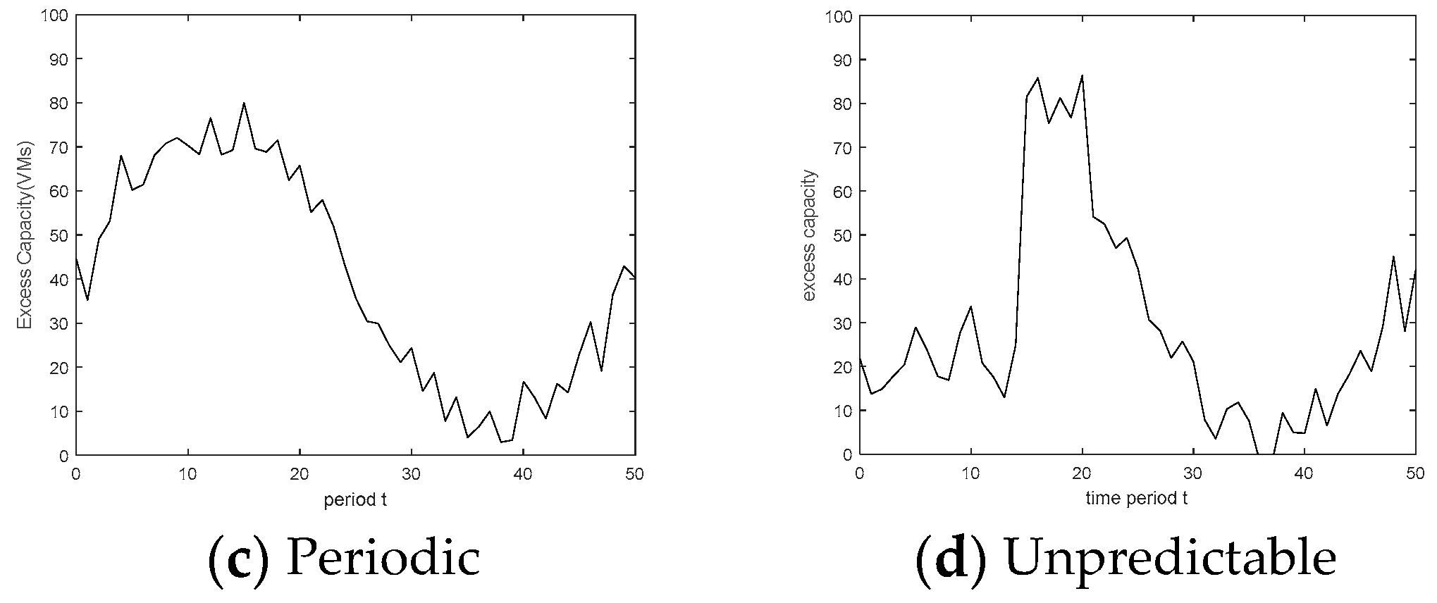
In this set of experiments, we consider synthetic non-stationary workload traces in which typical pattern changes occur alternately and are easy to detect. According to the literature [15], the workload of regular cloud service is mainly characterized by four basic non-stationary patterns: on-and-off, growing, periodic (e.g., sine curve), and unpredictable. Excess capacity is resource capacity after satisfying the workload of regular cloud services. Therefore, we simulate the non-stationary CPU excess capacity trace based on the above four basic non-stationary workload patterns.
We assume that there are 100 virtual machines in total and there is 1 CPU per virtual machine. c t denotes the CPU excess capacity available to spot services in period t. Subsequently, c t = N u t , where u t is the CPU usage of regular cloud services in period t. According to the non-stationary patterns of the CPU usage for regular cloud services, we simulate the non-stationary patterns of time-varying CPU excess capacity, c t , with Gaussian noise, which are shown in Figure 1a–d. Figure 1a shows an on-and-off structure which includes two linear patterns. One is simulated by c t = 20 + ε , where t {1, 2, …, 20} and t {36, 37, …, 50}; the other is simulated by c t = 70 + ε , where t {21, 22, …, 35}. There are two changepoints in this on-and-off pattern, t = 21 and t = 36. Figure 1b shows a decreasing structure, including three linear patterns, which is the combination of c t = 70 + ε , where t {1, 2, …, 14}, c t = 70 − 2 × t + ε , where t {15, 16, …, 35}, and c t = 10 + ε , where t {36,37,…,50}. There is no changepoint in this pattern. Figure 1c shows a periodic structure, including three linear patterns, which is simulated by a sine curve characterized as c t = 35 × (sin(( π /25) ×  t) + 40, where t {1, 2, …, 50}. There are two changepoints in this pattern. Figure 1d shows an unpredictable structure, including four linear patterns, which is the stochastic combination of the above non-stationary structures. The Gaussian noise term, ε , follows N ( 0 , 5 2 ) . There are three changepoints in this pattern. Note that the linear pattern denotes the pattern detected by our changepoint detection method.
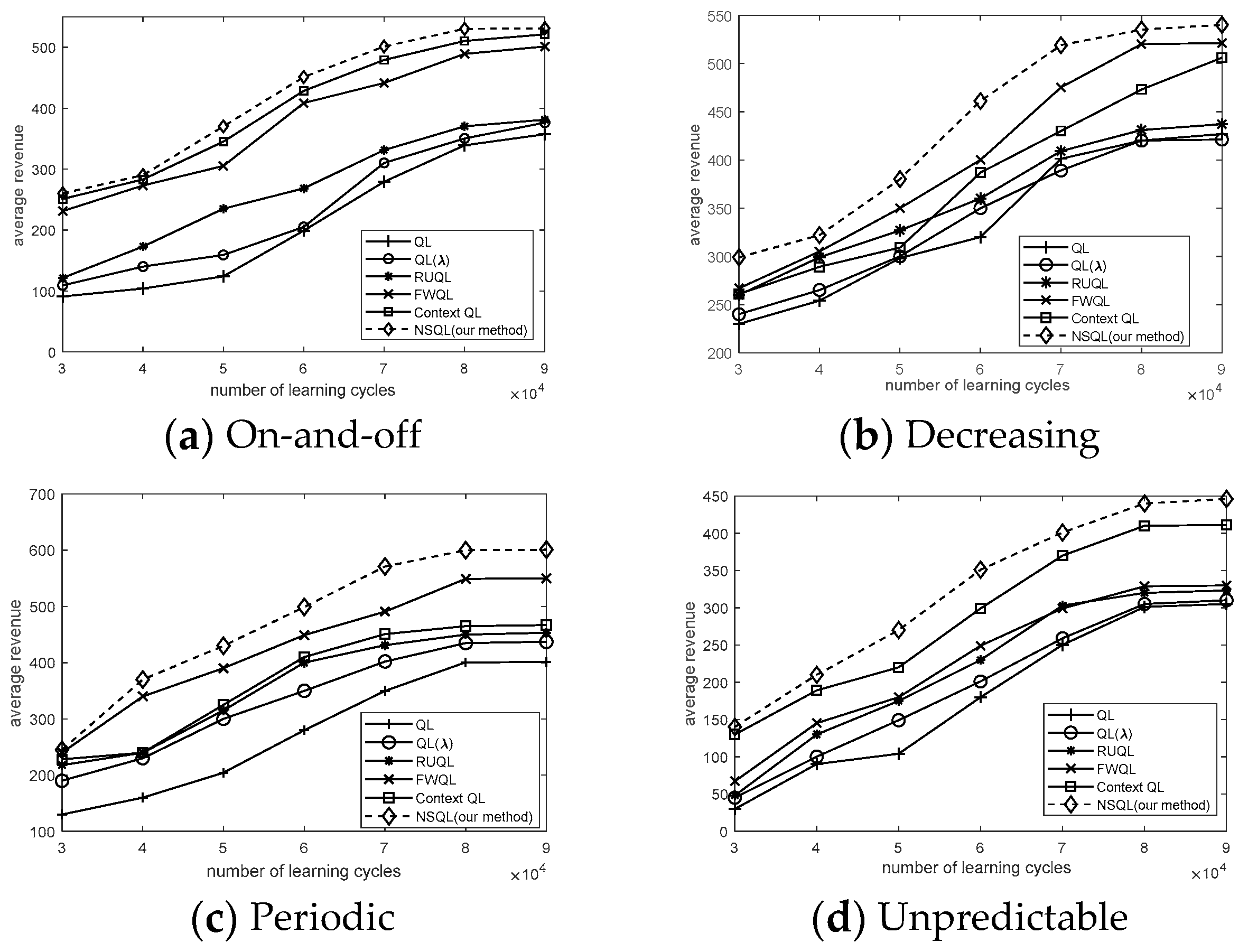
Note that the simulated time series of non-stationary excess capacity is unknown to the decision maker in our experiment validation and is only used as a simulation environment. For example, excess capacity in period t will be generated according to the simulated time series after the spot service price in period t is made. We compare the learning efficiency of the proposed algorithm (NSQL) with classical QL, repeated update QL (RUQL) [23], Q(λ) [26], FWQL [24], and context QL [25] in four simulated scenarios in Figure 1a–d. Classical QL does not deal with non-stationarity. Q(λ) uses eligibility traces, and FWQL restarts the Q-value according to the fixed-window size, so as to solve the non-stationary problem. RUQL [23] is similar to QL, but its exploration strategy and step size schedule differ from QL. Other details of these RUQL, FWQL, and Q(λ) algorithms can be found in the literature [23,24,26]. The above four QL algorithms do not detect changepoints, unlike our proposed NSQL (as described in Algorithm 1). Context QL, as described in the literature [25], has multivariate changepoint detection for the experience trace, different from our method, which just detects non-stationary univariate data. For the algorithms that involve hyperparameters (such as the learning rate, δ , discount factor, γ , exploration rate, ε , and fixed-window size of FWQL), we performed a grid search to choose the best value that maximizes the total revenue with δ = 0.3, γ = 0.99, and ε = 0.3. As shown in Figure 2, each point represents the average revenue of 10,000 simulated selling horizons, T, in which the spot prices are made by the Q-value table learned from a different number of learning cycles.
From Figure 2a–d, all of the methods designed for non-stationary excess capacity outperform classical QL, Q(λ), and RUQL, which do not explicitly model the changes in excess capacity over time from the convergence and average revenue. For example, as shown in Figure 2a, the learning process of our NSQL algorithm becomes stable at around 80,000 learning cycles, but the classic Q-learning is not convergent, even after 90,000 learning cycles. For classical Q-learning, the reason for its slower convergence is that there is a need to search the large space of non-stationary policies for learning the spot pricing policy in non-stationary environments. Therefore, an exhaustive search over this large space is computationally expensive and requires a higher number of iterations to obtain higher revenue. Different from classical QL, Q(λ), and RUQL, our NSQL algorithm can find an approximately optimal policy over a smaller, restricted set, which narrows the search space, resulting in higher revenue levels with faster convergence. Furthermore, from the results shown in Figure 2a–d, it is clear that NSQL significantly outperforms the other non-stationary algorithms, which are FWQL and context QL. For the context QL method, although both algorithms detect changepoints of non-stationary environments, context QL detects pattern changepoints based on the experience data generated during interactions with the environments. For non-stationary environments with noise, the experience data fluctuate greatly, and find it difficult to be accurate in identifying the points of change. This makes the detection of changepoints through experience data less effective than the detection of a non-stationary univariate.

4.3. Experiments on Real-World Non-Stationary Traces

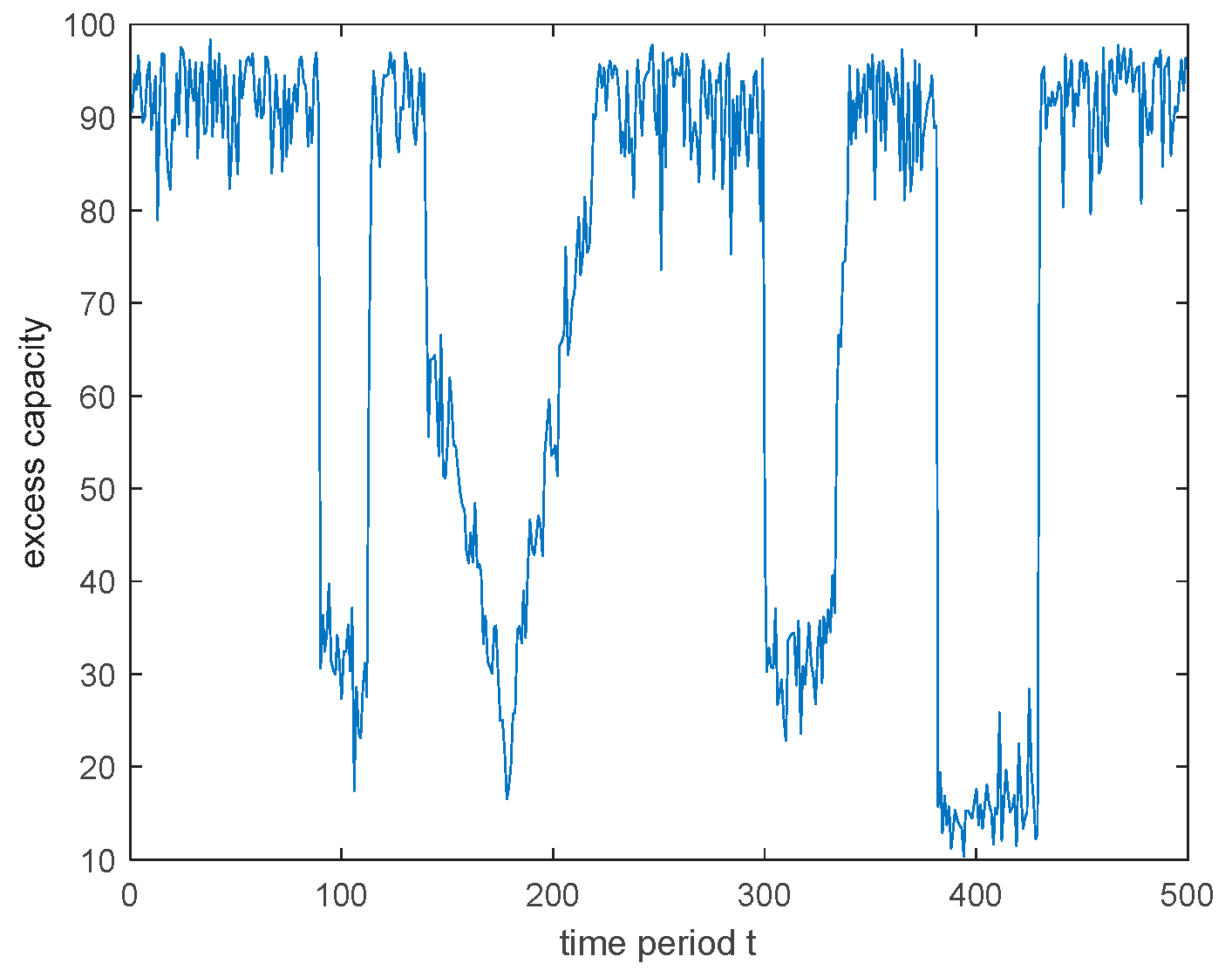
In this set of experiments, we employed a widely used workload dataset from the Microsoft Azure Compute Cluster [33], which represents the CPU utilization of two million regular VMs. By deducting the CPU utilization from the total amount of virtual computing resources, we obtain the CPU excess resource capacity. In this dataset, the average percent CPU utilization per VM is reported every five minutes. We examined 2045 of them and identified a VM cluster that includes 125 VMs. We displayed a set of 100 candidate VM traces of them over nearly 48 h. We assume 1 CPU for each VM. So, CPU utilization can be seen as CPU consumption. We sum the CPU utilization of 100 VMs and obtain the total CPU excess capacity of the 100 VMs, which is displayed in Figure 3. As is shown in Figure 3, the CPU excess capacity of the VM cluster fluctuates with time, and the fluctuation has certain regularity. That is, the mean value of the CPU excess capacity fluctuates and changes suddenly to another value, which shows extreme non-stationary behavior. We set the interval of each time period t to be 5 min, and there are 500 time periods in the whole time horizon T.
As is shown in Figure 3, the X-axis shows the time periods (five minutes per period) over 48 h, and the Y-axis shows the CPU excess capacity of the VM cluster. From the non-stationary characteristics, we can infer that it is likely that the VM cluster is hosting a restaurant service. When the time periods are between t = 1 and t = 90, the CPU excess capacity is at a high level, indicating that it is not peak dining time and that there are few diners. Thus, there is little workload on virtual machines in this time period. We can infer that this time period is at midnight. When the time periods are between t = 91 and t = 114, the CPU excess capacity is at a low level, which represents an increase in the number of diners, and there is a heavy workload on VMs during this time period. We can infer that these time periods are breakfast time. By analogy, we can explain the meaning of peaks and troughs in other time periods. In summary, these abrupt peak–trough changes represent transitions in the workload on VMs. Notice that the non-stationarity has visible and distinct sudden changes in its CPU excess capacity and has a time-dependent mean, which gives strong evidence for utilizing changepoint detection.
Due to the strong volatility of time-varying excess resources in the real-world dataset, the collected revenue has a high fluctuation. Therefore, we use the mean value, standard deviation (SD), and median of the collected revenue to describe the performances of the algorithms. Note that the real-world time series of non-stationary excess capacity is unknown to the decision maker and is only used as a generation for CPU excess capacity. So, the changepoint detection method is needed for the identification of pattern changepoints. Other parameters in our algorithm have the same settings as the experiment in Section 4.2. The performances of classical QL, Q(λ), RUQL, FWQL, context QL, and NSQL (our method) trained by 80,000 learning cycles are as follows.
From Table 1, the non-stationary algorithms, FWQL, context QL, and NSQL outperform the other algorithms without considering non-stationary changes. Additionally, we can see that the average revenue under NSQL (our method) and context QL with changepoint detection outperforms FWQL without a changepoint detection method. Compared to context QL, NSQL not only has a higher mean value of revenue but also has strong stability in terms of revenue level. The reason is that changepoint detection for non-stationary excess capacity is much better than changepoint detection for the experience tuple of the reinforcement learning process.

4.4. Comparison with Different Volatilities of Non-Stationary Excess Capacity

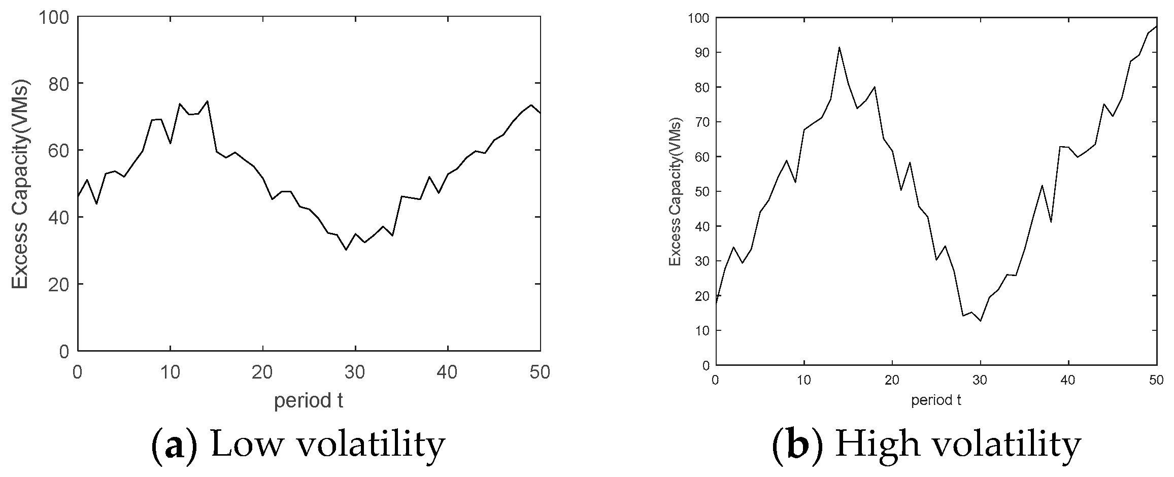
In this section, we further examine the effect of the volatility of non-stationary excess capacity using our method (NSQL). As are shown in Figure 4, two simulated non-stationary scenarios ((a) and (b)) are introduced, which have the same amount of excess capacity with different volatilities. Scenario (a): Peak-to-trough fluctuation with low volatility, which is shown in Figure 4a. The first pattern is simulated by c t = 45 + 2 ×  t + ε 1 , where t {1, 2, …, 15}; the second pattern is simulated by c t = 60 − (t − 15) × 2 + ε 2 , where t {16, 17, …, 30}; and the third pattern is simulated by c t = 33 + (t − 30) × 2 + ε 3 , where t {31, 32, …, 50}. The Gaussian noise terms, ε 1 , ε 2 , and ε 3 , follow N ( 0 , 5 ) . Scenario (b): Peak-to-trough fluctuation with high volatility, which is shown in Figure 4b. The first pattern is in a continuous growth simulated by c t = 15 + 5 ×  t + ε 1 , where t {1, 2, …, 15}; the second pattern is a continuous decreasing simulated by c t = 85 − (t − 15) × 5 + ε 2 , where t {16, 17, …, 30}; and the third is in a continuous growth simulated by c t = 15 + (t − 30) × 4 + ε 3 , where t {31, 32, …, 50}. The Gaussian noise terms, ε 1 , ε 2 , and ε 3 , follow N ( 0 , 5 2 ) .
Once again, the simulated time series of non-stationary excess capacity is unknown to the decision maker and is only used as a simulation environment. For example, excess capacity in period t will be generated according to the simulated time series after the spot service price in period t is made. Figure 5 presents the optimal spot price, total demand, and cumulative revenue within one horizon, T, in two different scenarios.
Figure 5a shows that the higher the volatility of non-stationary excess capacity, the more frequently the price of spot cloud services changes. In addition, we can observe that the optimal price decreases with the excess capacity increasing, and the optimal price increases with the excess capacity decreasing. The reason is that lower prices can increase revenue when the excess capacity is plentiful and higher prices can reduce service interruption risk when the excess capacity is scarce. In a highly volatile scenario, such frequent price changes have better performance in peak shaving and valley filling (presented in Figure 5b). When excess capacity in the operator is at a high level, a lower spot service price is adopted; when excess capacity is low, a higher spot price is adopted. Therefore, the spot pricing learned by our method can adapt to the dynamic volatility of excess capacity without interrupting spot service resources. Figure 5c shows that the higher the volatility of non-stationary excess capacity, the lower the cumulative revenue of spot services. Therefore, in order to maximize the total revenue of cloud resources, operators can reduce fluctuations in excess capacity by reasonably scheduling cloud computing workloads of on-demand and reserved services. For example, in peak times of resource demand, computing workloads with a strong time sensitivity can be served first, and computing requests with a low time sensitivity can be served in the trough period of computing workloads, so as to minimize the volatility of excess capacity, thereby maximizing the total cloud revenue.

5. Conclusions

In this paper, a non-stationary real-time pricing method for spot cloud services with non-stationary excess capacity is presented. Due to the non-stationarity of excess capacity, spot cloud services with pre-emption using real-time pricing were implemented to maximize cloud revenue. Focusing on the spot market segment in which users can tolerate service interruptions, a non-stationary MDP model was formulated. In this model, non-stationary excess capacity is partitioned into the piecewise linear pattern. The non-stationary MDP model fully embodies spot demand dynamic updating with service interruptions, considering non-stationary excess capacity. To solve the stochastic non-stationary problem with incomplete non-stationary excess capacity (without transition probabilities), Q-learning, the most popular and classical reinforcement learning algorithm, was adopted, and a new non-stationary Q-learning (NSQL) algorithm with burst pattern changepoint detection is proposed. A change detection method was used to determine changes in excess capacity and determine the pattern model in conjunction with Q-learning. With the aid of real-time interactions, the proposed Q-learning algorithm adaptively decides real-time spot prices during the online learning process. The simulation results show that the proposed method and algorithm perform well in varying non-stationary excess capacity conditions and give better returns when compared to classical Q-learning and other non-stationary learning algorithms, such as FWQL and context QL.
Future extensions to this work can focus on improving the accuracy of peak–trough detection in the context of large and continuous non-stationary excess capacity models. Such extensions may be useful in recognizing pattern changes in order to better adapt to extremely non-stationary environments.

Author Contributions

Conceptualization, Y.C. and H.P.; methodology, Y.C.; software, H.P.; validation, H.P., Y.C. and X.L.; formal analysis, H.P.; investigation, H.P.; data curation, H.P.; writing—original draft preparation, H.P.; writing—review and editing, X.L.; visualization, H.P.; supervision, Y.C. All authors have read and agreed to the published version of the manuscript.

Funding

This research received no external funding.

Institutional Review Board Statement

Not applicable.

Informed Consent Statement

Not applicable.

Data Availability Statement

Not applicable.

Acknowledgments

This work was finished when Huijie Peng was a visiting student at the National University of Singapore. The support provided by the East China University of Science and Technology during the visit of Huijie Peng to the National University of Singapore is acknowledged.

Conflicts of Interest

The authors declare no conflict of interest.

References

  1. Maghakian, J.; Comden, J.; Liu, Z. Online optimization in the Non-Stationary Cloud: Change Point Detection for Resource Provisioning. In Proceedings of the 53rd Annual Conference on Information Sciences and Systems, Baltimore, MD, USA, 20–22 March 2019. [Google Scholar]
  2. Kepes, B. 30% of Servers are Sitting “Comatose” according to Research. 2015. Available online: https://www.forbes.com/sites/benkepes/2015/06/03/30-of-servers-are-sitting-comatose-according-to-research/?sh=724cb7ea59c7 (accessed on 10 July 2022).
  3. Barr, J. Cloud Computing, Server Utilization, & the Environment|AWS News Blog. 2015. Available online: https://aws.amazon.com/blogs/aws/cloud-computing-server-utilization-the-environment/ (accessed on 11 July 2022).
  4. Greenberg, A.; Hamilton, J.; Maltz, D.A.; Patel, P. The cost of a cloud: Research problems in data center networks. ACM SIGCOMM Comput. Commun. 2008, 39, 68–73. [Google Scholar] [CrossRef]
  5. St-Onge, C.; Kara, N.; Wahab, O.A.; Edstrom, C.; Lemieux, Y. Detection of time series patterns and periodicity of cloud computing workloads. Future Gener. Comput. Syst. 2020, 109, 249–261. [Google Scholar] [CrossRef]
  6. Davidow, D.M. Analyzing Alibaba Cloud’s Preemptible Instance Pricing. Ph.D. dissertation, University of Haifa, Israel, 2021. [Google Scholar]
  7. Agmon Ben-Yehuda, O.; Ben-Yehuda, M.; Schuster, A.; Tsafrir, D. Deconstructing Amazon EC2 Spot Instance Pricing. ACM Trans. Econ. Comput. 2013, 1, 1–20. [Google Scholar] [CrossRef]
  8. George, G.; Wolski, R.; Krintz, C.; Brevik, J. Analyzing AWS Spot Instance Pricing. In Proceedings of the IEEE International Conference on Cloud Engineering, Prague, Czech Republic, 24–27 June 2019. [Google Scholar]
  9. Xu, H.; Li, B. Dynamic Cloud Pricing for Revenue Maximization. IEEE Trans. Cloud Comput. 2013, 1, 158–171. [Google Scholar] [CrossRef]
  10. Alzhouri, F.; Agarwal, A.; Liu, Y. Maximizing Cloud Revenue using Dynamic Pricing of Multiple Class Virtual Machines. IEEE Trans. Cloud Comput. 2021, 9, 682–695. [Google Scholar] [CrossRef]
  11. Lei, Y.M.; Jasin, S. Real-Time Dynamic Pricing for Revenue Management with Reusable Resources, Advance Reservation, and Deterministic Service Time Requirements. Oper. Res. 2020, 68, 676–685. [Google Scholar] [CrossRef]
  12. Bonacquisto, P.; Modica, G.D.; Petralia, G.; Tomarchio, O. A Procurement Auction Market to Trade Residual Cloud Computing Capacity. IEEE Trans. Cloud Comput. 2015, 3, 345–357. [Google Scholar] [CrossRef]
  13. Masdari, M.; Khoshnevis, A. A survey and classification of the workload forecasting methods in cloud computing. Cluster Comput. 2020, 23, 2399–2424. [Google Scholar] [CrossRef]
  14. Baig, S.R.; Iqbal, W.; Berral, J.L.; Carrera, D. Adaptive sliding windows for improved estimation of data center resource utilization. Future Gener. Comput. Syst. 2020, 104, 212–224. [Google Scholar] [CrossRef]
  15. Nikravesh, A.Y.; Ajila, S.A.; Lung, C.H. An autonomic prediction suite for cloud resource provisioning. J. Cloud. Comput Adv. S 2017, 6, 3. [Google Scholar] [CrossRef] [Green Version]
  16. Palshikar, G.K. Simple Algorithms for Peak Detection in Time-Series. In Proceedings of the 1st IIMA International Conference on Advanced Data Analysis, Business Analytics and Intelligence, Ahmedabad, India, 6–7 June 2009. [Google Scholar]
  17. Tahir, F.; Abdullah, M.; Bukhari, F.; Almustafa, K.M.; Iqbal, W. Online Workload Burst Detection for Efficient Predictive Autoscaling of Applications. IEEE Access 2020, 8, 73730–73745. [Google Scholar] [CrossRef]
  18. Sutton, S.R.; Barto, A.G. Reinforcement Learning: An Introduction, 2nd ed.; MIT Press: Cambridge, England, 2018; pp. 97–113. [Google Scholar]
  19. Cheng, Y. Dynamic packaging in e-retailing with stochastic demand over finite horizons: A Q-learning approach. Expert. Syst. Appl. 2009, 36, 472–480. [Google Scholar] [CrossRef]
  20. Gosavii, A.; Bandla, N.; Das, T.K. A reinforcement learning approach to a single leg airline revenue management problem with multiple fare classes and overbooking. IIE Trans. 2002, 34, 729–742. [Google Scholar] [CrossRef]
  21. Zhang, L.; Gao, Y.; Zhu, H.; Tao, L. A distributed real-time pricing strategy based on reinforcement learning approach for smart grid. Expert. Syst. Appl. 2022, 191, 116285. [Google Scholar] [CrossRef]
  22. Alsarhan, A.; Itradat, A.; Al-Dubai, A.Y.; Zomaya, A.Y.; Min, G. Adaptive Resource Allocation and Provisioning in Multi-Service Cloud Environments. IEEE Trans. Parall. Distr. 2018, 29, 31–42. [Google Scholar] [CrossRef]
  23. Abdallah, S. Addressing Environment Non-Stationarity by Repeating Q-learning Updates. J. Mach. Learn. 2016, 17, 1582–1612. [Google Scholar]
  24. Mao, W.; Zhang, K.; Zhu, R.; Simchi-Levi, D.; Basar, T. Near-optimal model-free reinforcement learning in non-stationary episodic mdps. In Proceedings of the 38th International Conference on Machine Learning, Virtual, 18–24 July 2021. [Google Scholar]
  25. Padakandla, K.S.; Bhatnagar, S. Reinforcement learning algorithm for non-stationary environments. Appl. Intell. 2020, 50, 3590–3606. [Google Scholar] [CrossRef]
  26. Rana, R.; Oliveira, F.S. Real-time dynamic pricing in a non-stationary environment using model-free reinforcement learning. Omega 2014, 47, 116–126. [Google Scholar] [CrossRef]
  27. Rana, R.; Oliveira, F.S. Dynamic pricing policies for interdependent perishable products or services using reinforcement learning. Expert. Syst. Appl. 2015, 42, 426–436. [Google Scholar] [CrossRef]
  28. Lin, L.; Pan, L.; Liu, S. Methods for improving the availability of spot instances: A survey. Comput. Ind. 2022, 141, 103718. [Google Scholar] [CrossRef]
  29. Chen, S.; Moinzadeh, K.; Tan, Y. Discount schemes for the preemptible service of a cloud platform with unutilized capacity. Inform. Syst. Res. 2021, 32, 967–986. [Google Scholar] [CrossRef]
  30. Watkins, J.C.; Dayan, P. Q-learning. Mach. Learn. 1992, 8, 279–292. [Google Scholar] [CrossRef]
  31. Richman, J.S.; Moorman, J.R. Physiological time-series analysis using approximate entropy and sample entropy. Am. J. Physiol-Heart C 2000, 278, 2039–2049. [Google Scholar] [CrossRef] [PubMed]
  32. Zharikov, E.; Telenyk, S.; Bidyuk, P. Adaptive workload forecasting in cloud data centers. J. Grid Comput. 2020, 18, 149–168. [Google Scholar] [CrossRef]
  33. Cortez, E.; Bonde, A.; Muzio, A.; Russinovich, M.; Fontoura, M.; Bianchini, R. Resource central: Understanding and predicting workloads for improved resource management in large cloud platforms. In Proceedings of the 26th Symposium on Operating Systems Principles, Shanghai, China, 28 October 2017; pp. 153–167. [Google Scholar]
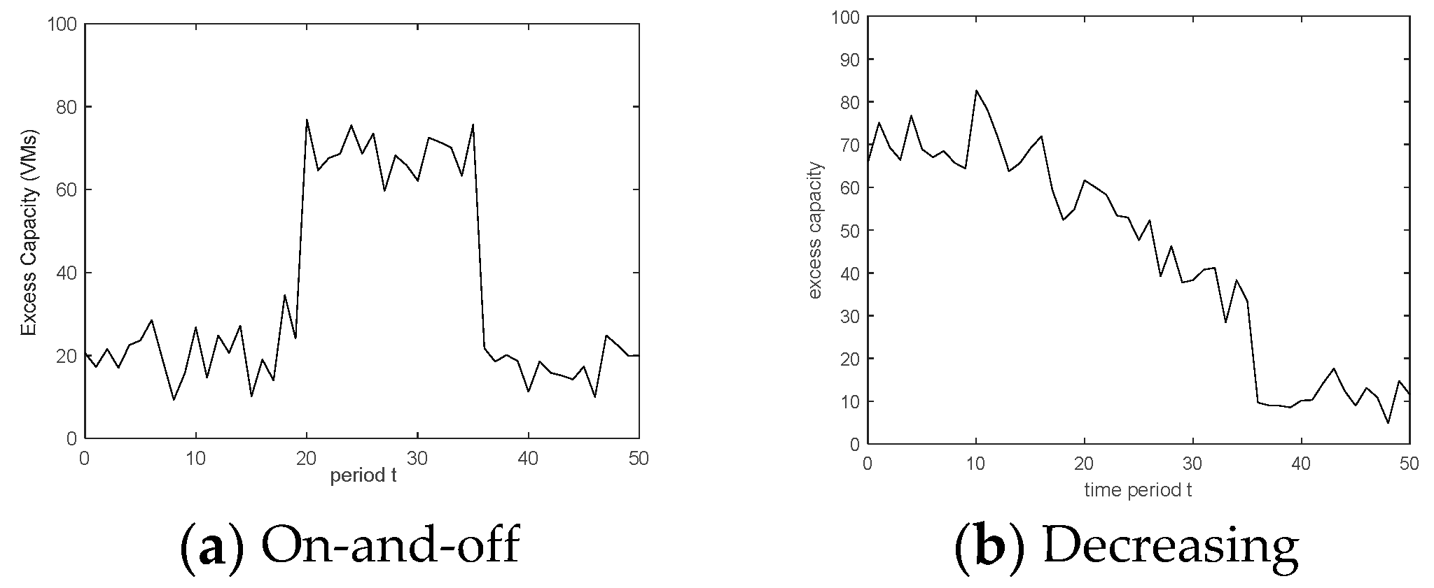
Figure 1. Four simulated non-stationary scenarios for time-varying excess capacity.
Sustainability 15 03363 g001aSustainability 15 03363 g001b
Figure 2. Comparisons of the average revenue in four non-stationary scenarios.
Sustainability 15 03363 g002
Figure 3. The real-world non-stationary trace of CPU excess capacity in T = 500.
Sustainability 15 03363 g003
Figure 4. Two simulated non-stationary scenarios with different volatilities.
Sustainability 15 03363 g004
Figure 5. Comparison with different volatilities of non-stationary excess capacity.
Sustainability 15 03363 g005
Table 1. Rewards collected by different methods based on the real-world dataset.
MethodMean ± SDMedian
NSQL (our method)4074.12 ± 55.154083.06
Context QL3850 ± 103.133865.12
FWQL3656 ± 125.13660.89
RUQL3380.23 ± 88.993401.31
Q(λ)3351.14 ± 69.13353.67
QL3039 ± 71.33042.19
Disclaimer/Publisher’s Note: The statements, opinions and data contained in all publications are solely those of the individual author(s) and contributor(s) and not of MDPI and/or the editor(s). MDPI and/or the editor(s) disclaim responsibility for any injury to people or property resulting from any ideas, methods, instructions or products referred to in the content.