Article

Multi-Objective Optimal Power Flow Calculation Considering Carbon Emission Intensity

1
College of Energy and Electrical Engineering, Qinghai University, Xining 810016, China
2
Hubei Engineering and Technology Research Center for AC/DC Intelligent Distribution Network, School of Electrical Engineering and Automation, Wuhan University, Wuhan 430072, China
3
School of Electrical and Automation, Wuhan University, Wuhan 430072, China
4
Department of Electrical Engineering, College of Engineering at Wadi Addawasir, Prince Sattam bin Abdulaziz University, Wadi Addawasir 11991, Saudi Arabia
5
Department of Electrical & Computer Engineering, University of Denver, Denver, CO 80210, USA
6
School of Electrical Engineering, Xi’an University of Technology, Xi’an 710054, China
*
Author to whom correspondence should be addressed.
Sustainability 2023, 15(24), 16953; https://doi.org/10.3390/su152416953
Submission received: 31 October 2023 / Revised: 8 December 2023 / Accepted: 12 December 2023 / Published: 18 December 2023

Abstract

:
In keeping with China’s dual carbon goals, optimal low-carbon power system dispatch has become a necessary component of the greening of the power system. However, typically, research considers only the economics of such efforts. Based on our power flow analysis of the power grid and the correlation properties of carbon emission flow, an optimal power flow calculation model targeting the total carbon emission rate of the power system’s power generation cost, active network loss, and load and network loss was constructed. Next, the NSGA-III algorithm was used to solve the model, and the decision was to coordinate and optimize the output schemes of various types of power plants, such as wind, water, and thermal. The modified IEEE39 node simulation system was built with Matlab software (MATLAB R2020b). The results of the calculation showed that, compared to the traditional method of determining the optimal power flow, the proposed method reduced the system carbon emissions by 20% while the power generation cost increased by less than 2%, which proves the effectiveness and practicability of the proposed method.

1. Introduction

Greenhouse gas emissions (GHG) have emerged as a global concern hindering societal progress. Recognizing this challenge, the international community is unified in its drive to foster the development of a low-carbon economy and enhance the optimization of the energy composition. During the general debate of the 75th session of the United Nations General Assembly on the 22 September 2020, President Xi Jinping of China declared that China is committed to attaining the pinnacle of carbon emissions before 2030 and aims to achieve carbon neutrality by 2060 [1]. As of the conclusion of 2021, China, being one of the largest power consumers, boasted an installed power generation capacity of 2.38 billion kW. Thermal power constituted 56.58% of this total capacity [2]. According to statistics, the power industry’s share of national carbon emissions has reached 50% [3]. According to the predictions in the literature [4], the Chinese power sector can achieve the goal of zero carbon dioxide emissions by 2050, with the completion of technology for capturing and storing carbon emissions [5], the transformation of thermal power units, and the utilization of mass renewable energy power generation. The power industry holds immense potential for reducing CO2 emissions. The transition to a low-carbon power system will greatly promote the realization of China’s dual-carbon goals [6]. Therefore, a thorough analysis of carbon emissions, coupled with generation costs, is essential in the operation of power systems. This will allow for the judicious use of renewable power resources [7], driving power systems closer to their low-carbon and economic objectives.
For power systems to realize green and low-carbon electricity dispatch, it is crucial to concurrently weigh the economic and reliability aspects of power dispatching [8] with the system’s CO2 emissions characteristics. In Li and Han [9], second-order Taylor expansion is used to correct the state variables once, and the corrected results are used to calculate the control variables and the output of the distributed energy sources. Using the sparse characteristics of the Hessian array, a distributed Gaussian elimination method is proposed to achieve a distributed solution for the distribution network optimal power flow. Zhang et al. [10], who endeavor to address active network loss, propose a method for optimal power flow calculation with controllable phase shifters based on the improved interior point method. Another relevant study is that of Zhu et al. [11], which establishes an uncertain optimal power flow model for evaluating the absorptive capacity of renewable distributed generation and a deterministic equivalent conversion method for an optimal power flow model under different description forms. Study [12] proposes an optimal power flow solution method for systems integrating solar photovoltaic and wind energy with traditional generators based on the hybrid particle swarm gray wolf optimizer (HPS-GWO). By analyzing the features of coal-fired power plants, Wang et al. [13] formulates a mathematical model depicting the correlation between carbon emissions and generator output, and proposes a dual-objective economical and low-carbon optimal scheduling method employing an algorithm that evolves weights adaptively. However, this broad approach to carbon emissions lacks the capability to analyze individual links within the system. Zhang et al. [14] introduces the cost associated with CO2 over-emissions and the generalized cost of wind power generation. To account for the influence of carbon emission quotas and the integration of wind power on system power generation costs, a day-ahead scheduling model is formulated, with the optimization objective being the minimization of the overall system power generation cost. Mei et al. [3] uses an aggregate allocation method to fairly allocate carbon emission rights, and then establishes a model for low-carbon electricity dispatch, taking into account the constraints imposed by carbon emission rights. But this allocation model is established on a macro level, and cannot conduct an in-depth analysis of carbon emissions in the power system. Han et al. [15] proposes a power system low-carbon scheduling strategy, taking into account flexible demand response and energy storage by combining a carbon emission index with a flexible resource scheduling model. In Li et al. [16], a dual-layer alternating optimal scheduling model is formulated, encompassing day-ahead dispatch and load demand response [17]. Additionally, in light of carbon capture systems and the theory of carbon emission flow, a low-carbon optimal learning and dispatching method for the power system is introduced. In Zhong et al. [18], a bi-level optimization model is proposed to guide users to actively choose green energy consumption. The higher level seeks to maximize the benefits of wind power, photovoltaic, and coal-fired power plants, and the lower level aims at minimizing the cost of electricity consumption, utilizing electricity prices and carbon responsibility as motivating factors. The carbon emissions in Jiang et al. [19] and Fakih et al. [20] are calculated based on fuel or typical energy carbon emission factors. This study exclusively investigates carbon emissions from the energy supply side and does not conduct an internal analysis of the system.
However, the above studies either only consider the economy and reliability of the power grid, or only analyze macro carbon emissions, and there is no micro study of every unit of the electrical grid. To deal with these problems, this paper optimizes the dispatch of the power system with the goals of economy and environmental protection. According to the unique traits of carbon emission flow, this paper analyzes the virtual carbon emission flow across different sections of the power grid. By establishing an optimal power flow model that prioritizes power generation cost, active network loss, and the overall carbon emission rate, the power generation strategy is devised by maximizing the utilization of renewable resources and reducing their carbon emissions. Finally, this paper takes the modified IEEE-39 node system as a demonstration to validate the efficacy and viability of the proposed approach.

2. Model Design and Calculation of Carbon Emission Flow in Power System

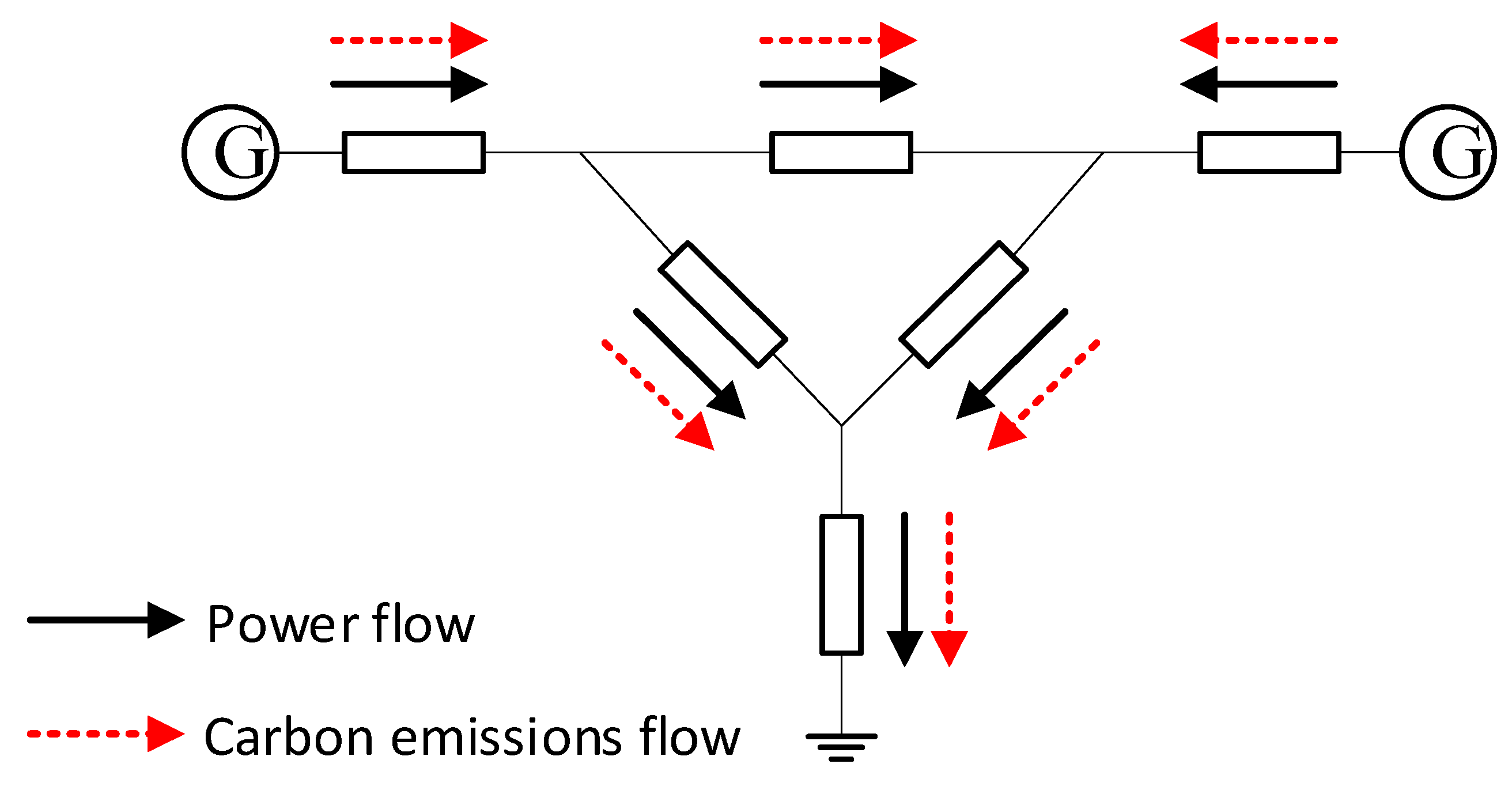
2.1. Carbon Emission Flow of Power System

The carbon emission flow of the power system refers to the flow process of the CO2 emissions generated during the production, transmission, and use of electricity. The carbon emission features of the power system are that emissions are concentrated at the power generation end and consumption is concentrated at the load end [21]. From the perspective of the energy transfer chain, carbon emissions are collected from the power generation side to the consumer end through the power flow. If the carbon emissions generated in the power production process are regarded as flowable, they flow to the load along with the power flow and are finally discharged into the atmosphere. The distribution of carbon emissions moving through the power system is called the carbon emission flow of the power system [22], which is also referred to as the carbon flow. The carbon flow of the power system is a virtual network flow attached to the power flow. It is shown in Figure 1. Carbon emission flow helps to analyze the carbon emissions of the power system and offers a theoretical foundation for the low-carbon transition of the electricity grid.

2.2. Basic Definition of Carbon Emission Flow in Power System

The theory of carbon flow in power systems utilizes several new terms that form the theoretical basis for its analysis; these are shown below.

2.2.1. Carbon Emission Flow

Also referred to as carbon flow, this refers to the total quantity of carbon emissions associated with the carbon emission flow traversing a node or branch of the power flow within a specific timeframe by the symbol F, as stated in tCO2.

2.2.2. Carbon Flow Rate

This indicates the carbon flow passing through a node or branch per unit time. It is represented by the symbol R, as stated in tCO2/h, which is mathematically equivalent to the derivative value of carbon flow with respect to time.
R = F t
where t is time, as stated in hour (h).

2.2.3. Branch Carbon Flow Density

The carbon flow of the electricity grid relies on the power flow. The carbon emissions generated by the generating plant side resulting from the transmission of unit electricity on the branch of the grid are collectively called the carbon flow density of the branch. It is alternatively defined as the proportion of the carbon flow rate to the active power of a branch within the power system. It is denoted by the symbol ρ, measured in units of tCO2/kWh.
ρ = R P
where P is the active power, as stated in kW.

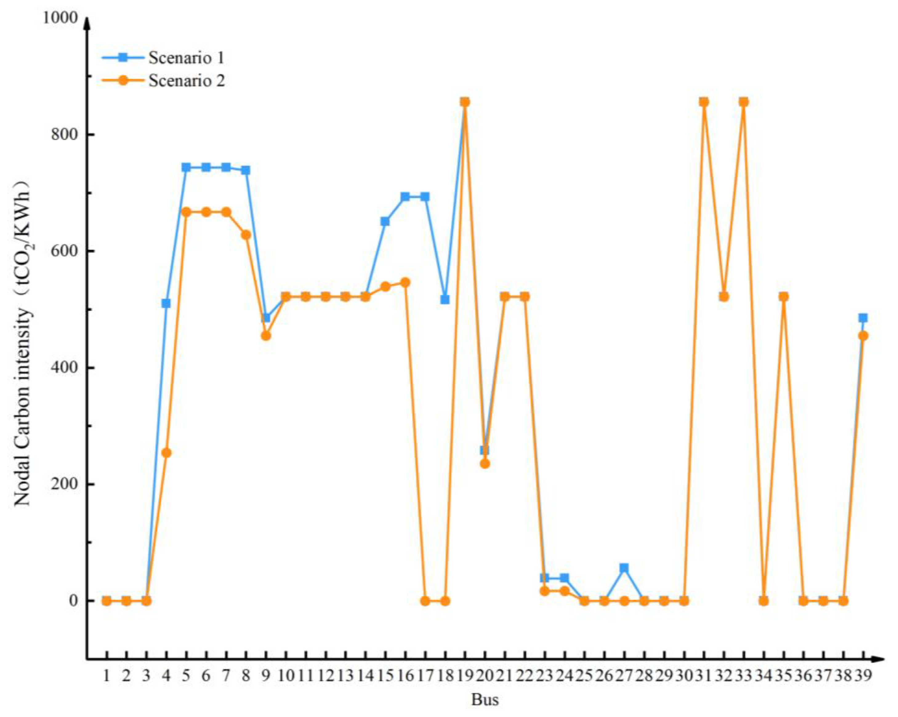
2.2.4. Nodal Carbon Intensity

The carbon emission of the power plant side caused by the consumption of unit electricity at the node side is the node carbon intensity, represented by e, measured in tCO2/kWh. On the power plant side, the carbon intensity at the node is equivalent to the carbon emission intensity of the power plant.
e = i N + P i ρ i i N + P i = i N + R i i N + P i
where N+ signifies the aggregation of all branches of the power flow directed into the node; i denotes the branch index.
In accordance with the principles of proportional sharing and energy conservation, any outflow power flow branch connected to the node contains all the components of the inflow power flow branch, and the carbon flow rate of the outflow power flow branch is equal to the sum of the carbon flow rates contributed by all the inflow power flow branches to the branch [23]. It can be obtained from (4), where the carbon flow density of all the branches flowing out of the from the node equals the carbon intensity of the node. In (4), ρ i j represents the carbon flow density of the branch from node i to node j, then ρ i j = e i , that is, the carbon flow density of the branch is equivalent to the carbon intensity of the originating node flowing into the branch.
ρ j , j N = i N + P j P i s N + P s ρ i P j = i N + P i ρ i s N + P s = s N + R s s N + P s = e

2.3. Calculation Method for Carbon Emission Flow in Power System

In the power flow analysis, one can compute the power flow distribution across all nodes and branches. Once the carbon potential of each node is known, the carbon emission flow rate for each branch can be determined based on the characteristics of the power system’s carbon emission flow and the results of the power flow calculations. Subsequently, solving for the entire system’s carbon emission flow becomes feasible [23,24]. Therefore, the primary objective in carbon emission flow calculation is the determination of the carbon potential for each node in the power system.
According to the definition of node carbon potential, the carbon potential of node n is:
e n = i N + P B i ρ i + P G n e G n i N + P B i + P G n
where P B i conveys the real power from branch i directed into node n, measured in kW; P G n denotes the real power injected by the power plant to node n, measured in kW; e G n represents the carbon emission intensity of generators at node n, with units of CO2/kWh; and ρ i denotes the branch carbon flow density of branch i, measured in tCO2/kWh.

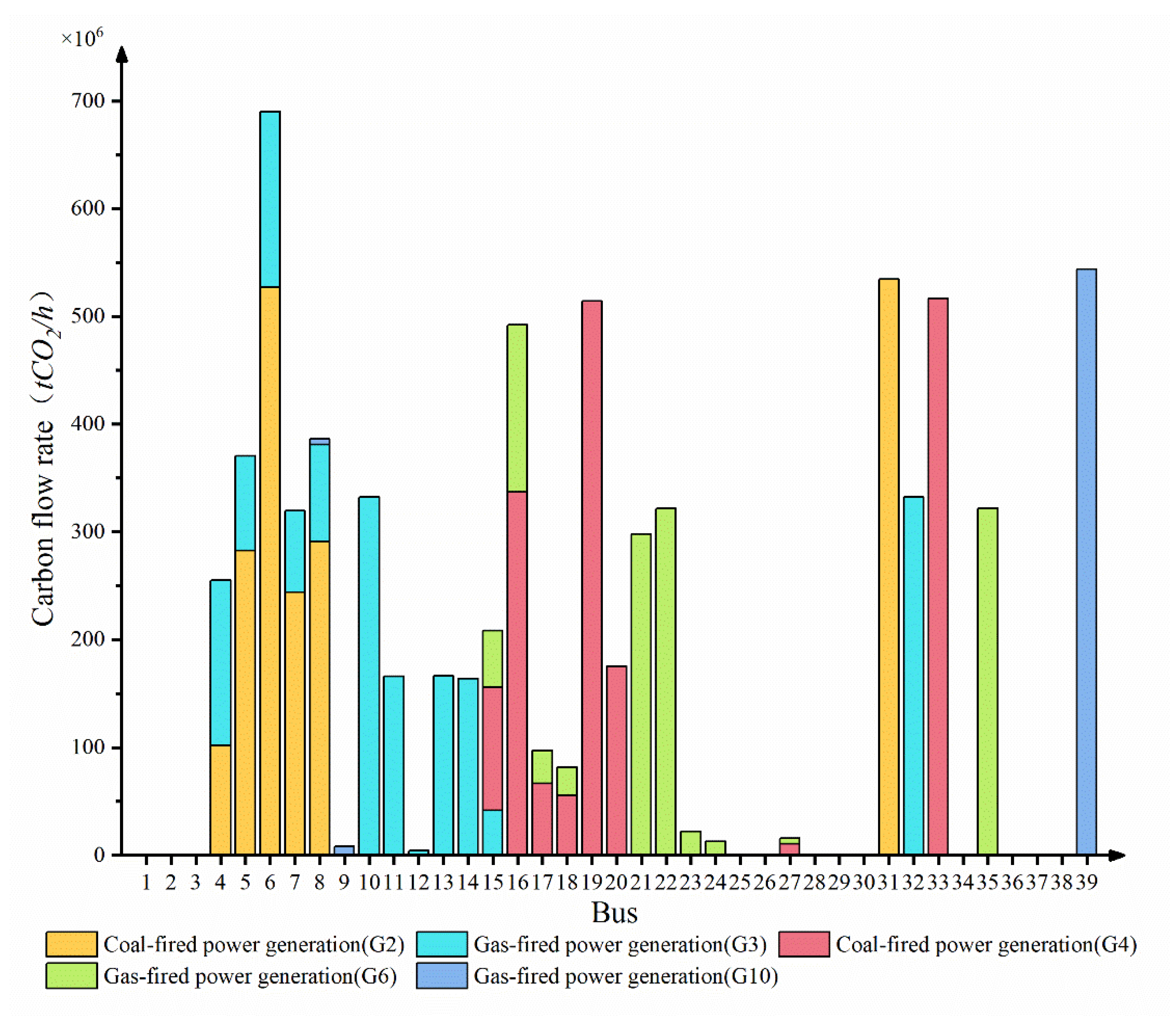
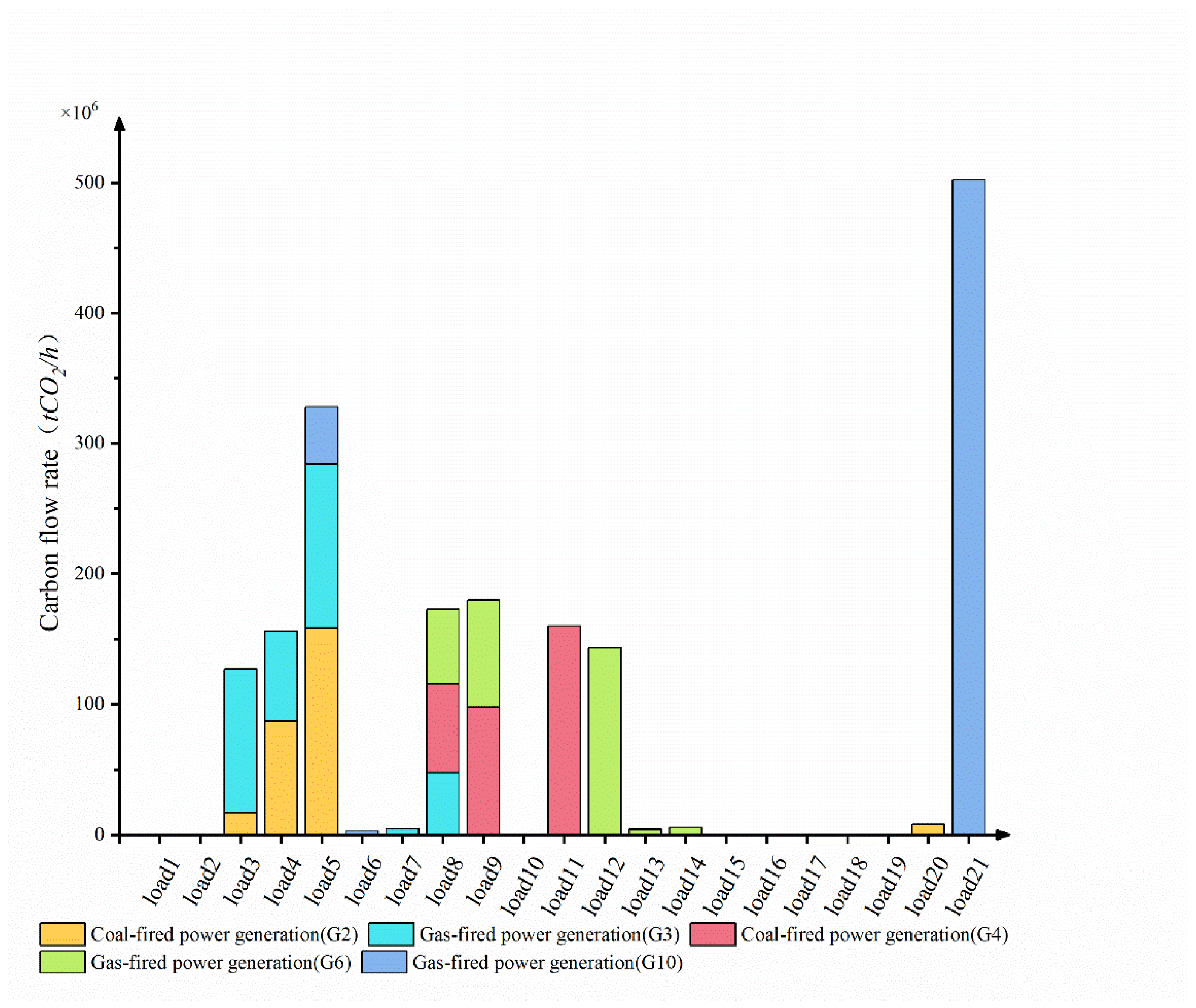
2.4. Correlation Analysis between Power Plant and Node Carbon Flow, Load Carbon Flow

As was established by [25], the carbon flow output distribution factor is equal to the power flow output distribution factor. The two are collectively referred to as the node output distribution factor.
H i j = H i j F = H i j P = R i j R i = P i j P i
where H i j , H i j F , and H i j P are node output distribution factors, carbon flow output distribution factors, and power flow output distribution factors from node i to node j, respectively; R i j is the carbon flow rate from node i to node j; R i represents the total carbon flow inflow from node i; P i j denotes the active power flow flowing from node i to node j; and P i is the total active power flow flowing into node i.
The path output distribution factor is determined by the proportion of the network flow departing from the source node compared to the total network flows entering the destination node [24]. Specifically, the path transmission distribution factor Dij signifies the flow distribution from node i to node j.
D i j = L γ ( ( m , n ) B L H m , n )
where (m, n) is a branch from node m to node n on the path L; BL is a path from node i to node j; and γ is a set of paths from node i to node j.
R G k , i represents the contribution of power plant k to the carbon flow rate at node i.
R G k , i = P G k e G k D k i
where P G k denotes the real power produced by power plant k; and e G k is the carbon emission intensity of power plant k.
R G k , L i represents the contribution of power plant k to the carbon flow rate at load i.
R G k , L i = R G k , i P L i P i
where P L i is the real power consumption of load i; and P i is the cumulative real power flow directed into node i.
In essence, following the principles of carbon emission flow theory, the carbon emission flow and carbon flow rate align with electricity and active power within the power flow context, respectively, bearing distinct physical interpretations. By formulating the theoretical framework of carbon emission flow, it becomes possible to compute the carbon emissions attributable to both load consumption and branch transmission within the system. This calculation relies on the power generation output and the power flow within the grid. Consequently, the original carbon emissions attributed solely to power generation are effectively distributed across various segments of the power system, adhering to a specific mechanism. This allocation provides a foundational framework for scrutinizing carbon emissions across the different segments of the power grid.

3. Optimal Power Flow Considering Carbon Emission Rate

As depicted in (10), the optimal power flow problem is a constrained optimization problem [26] which can be described as: under the condition that the network structure and parameters and the system load are given, various equality and inequality constraints [27,28] are satisfied, and one or several given objective functions describing the operating efficiency of the system are maximized, by determining the controllable variables of the system.
s . t . m i n ( f ( u , x ) ) g ( u , x ) = 0 h ( u , x ) 0
where min  f ( u , x ) is the objective function; g ( u , x ) = 0 is the equality constraint; h ( u , x ) 0 is the inequality constraint; u is the controllable variable, which usually includes the real power output and reactive power output (or terminal voltage) of each power plant, the tap position of the phase shifter, and the tap position of the voltage regulator; and x represents the state variable and the dependent variable of the controllable variable, which usually includes the node voltage and the power of each branch.

3.1. Objective Function

This paper studies the multi-objective optimal power flow in the power grid considering carbon emission intensity. The objectives include the lowest system power generation cost, the smallest real network loss, and the lowest total carbon flow rate. The mathematical model for each objective function is expressed as follows:
1.
Lowest cost of power generation:
m i n i = 1 N g e n ( a i 1 P G i + a i 0 )
where Ngen denotes the total number of power plants; P G i denotes the real power produced by power plant i; and a i 1 and a i 0 refer to the cost characteristic coefficients of power plant i.
2.
The lowest active network loss:
m i n i , j n b P i j + P j i
where n b is the collection of all branches.
3.
The lowest total carbon flow rate:
m i n ( i n l R L i + i n b R B i l o s s )
where n l is the collection of all loads; R L i represents the carbon flow rate consumed by the load i; and R B i l o s s indicates the carbon flow rate consumed by the real power loss on branch i.

3.2. Constraints

3.2.1. Equality Constraints

As depicted in (14) and (15), the optimal power flow denotes an optimized distribution of power flow, where adherence to the equality constraints of the fundamental power flow equations is necessary [29]. Additionally, considering the direction of the carbon flow from the power generation side to the consumer end for consumption, it is essential to maintain equilibrium between the injection and consumption of carbon emission flow.
P G i P L i U i j = 1 n U j ( G i j cos θ i j + B i j sin θ i j ) = 0
Q G i Q L i U i j = 1 n U j ( G i j sin θ i j B i j cos θ i j ) = 0
R G i R L i j = 1 j i n R i j , l o s s = 0
where n denotes the total number of nodes in the power grid; P G i and Q G i are the real power and reactive power generated by the power plant i, respectively; P L i and Q L i are the real load and reactive load at the bus i, respectively; G i j and B i j are the real part and imaginary part of the element in row i and column j of the node admittance matrix, respectively; θ i j is the phase difference between node i and node j, θ i j = θ i θ j ; U i and U j are amplitudes of voltage at node i and node j, respectively; R G i is the carbon flow rate injected into the system by power plant i; R L i is the carbon flow rate consumed by the load of bus i; and R i j , l o s s denotes the carbon flow rate of the network loss from node i to node j.

3.2.2. Inequality Constraints

To ensure the secure and reliable operation of the power system, the power plant is mandated to adhere to its operational upper and lower limits [30]. In addition, the voltage amplitudes and line capacities need to meet some requirements.
P G i , min P G i P G i , max
Q G i , min Q G i Q G i , max
U i , min U i U i , max
S i j S i j , max
where P G i , m i n and P G i , m a x are the upper and lower limits of the active power generated by the i-th generator; Q G i , m i n and Q G i , m a x are the upper and lower limits of the reactive power generated by the i-th generator; U i , m i n and U i , m a x are the upper limit and lower limit of the voltage amplitude of node i, respectively; and S i j , m a x denotes the upper limit of the line capacity of the branch from node i to node j.

3.3. Optimal Model Solution

3.3.1. NSGA-III Algorithm

NSGA-III (Non-dominated Sorting Genetic Algorithm III) is a multi-objective optimization algorithm, which is an improvement and extension of the classic NSGA-II algorithm [31]. The structure of NSGA-III closely mirrors that of NSGA-II, incorporating swift non-dominated sorting to categorize individuals within the population into distinct, non-dominated fronts. The divergence lies in the environmental selection within the critical layer, where NSGA-II preserves diversity through crowding comparison. The most significant alteration in NSGA-III involves the utilization of the minimum habitat mechanism to select optimal individuals through evenly distributed reference points to preserve population diversity [32]. The flowchart of the NSGA-III algorithm is illustrated in Figure A1 included in Appendix A. The implementation of NSGA-III is as follows:
  • Initialization. Set the basic variables of the NSGA-III algorithm, including the population size, mutation probability, number of iterations, and crossover probability, etc. Read the node, branch, and power plant data of the power grid. The initial population is obtained according to the constraints of the decision variables and the fitness function. Create a population archive set S.
  • Genetic manipulation. Perform selection, crossover, and mutation operations on the parental population to generate the offspring population Q.
  • Non-dominated sorting stratification. Merge the parental and offspring populations and execute fast non-dominated sorting, stratify according to the dominance level of the individual, and then put the individual into the archive set S layer by layer until the amount of individuals in set S is not less than the population size.
  • Selection of individuals in the critical layer based on reference point. In the NSGA-III algorithm, diversity within the population is preserved by incorporating evenly spread reference points. These reference points are utilized to choose individuals situated in the crucial layer, preventing the optimization process from being trapped in local optima. The pivotal layer within the archive set “S” is referred to as the “critical layer.” Assuming this layer is denoted as the “L-th” layer, the objective is to select “K” individuals from this critical layer (where “K” equals the population size minus the count of individuals present in the preceding “L − 1” layers within set “S”). These chosen individuals from the critical layer, along with individuals from the “L − 1” layer, together constitute a fresh population set.
  • Continue Steps 2 to 4 until the prescribed number of iterations is reached. Finally, output the Pareto front [33].

3.3.2. Pareto Optimal Set Decision Making

In this paper, the importance of each index is highlighted by assigning specific weights to individual objectives. Subsequently, the TOPSIS method is used to evaluate and sort each solution within the Pareto optimal solution set for the selection of the optimal solution [34,35]. The detailed procedure is outlined as follows:
  • Obtain a collection of optimal Pareto solution sets through the NSGA-III algorithm, that is, the indicator matrix P(m,n) (suggesting that there are a total of m solutions, with each solution comprising n indicators), and subsequently allocate a weight αn to each indicator within the solution set n (indicates that the weight of the nth index is αn).
  • Standardize the indicator matrix and assign weights to each element to derive the weighting matrix K.
The standardized index matrix is:
P ( m , n ) = P ( m , n ) m a x ( P ( : , n ) )
The weighting matrix is:
K ( m , n ) = P ( m , n ) × α n
3.
Consider the minimum element in each column of the weighting matrix as the optimal solution for index n, denoted as P n + , and the maximum element as the worst solution for index n, denoted as P n . Compute the distance of each solution in the weighting matrix to the optimal and worst solutions, denoted as, Z m + and Z m , respectively.
Z m + = i = 1 n K ( m , n ) P n + 2 Z m = i = 1 n K ( m , n ) P n 2
4.
Compute the proximity index R for each solution within the Pareto solution set with respect to the optimal level. Select the solution corresponding to the maximum R value as the objective function value to achieve optimal power flow.
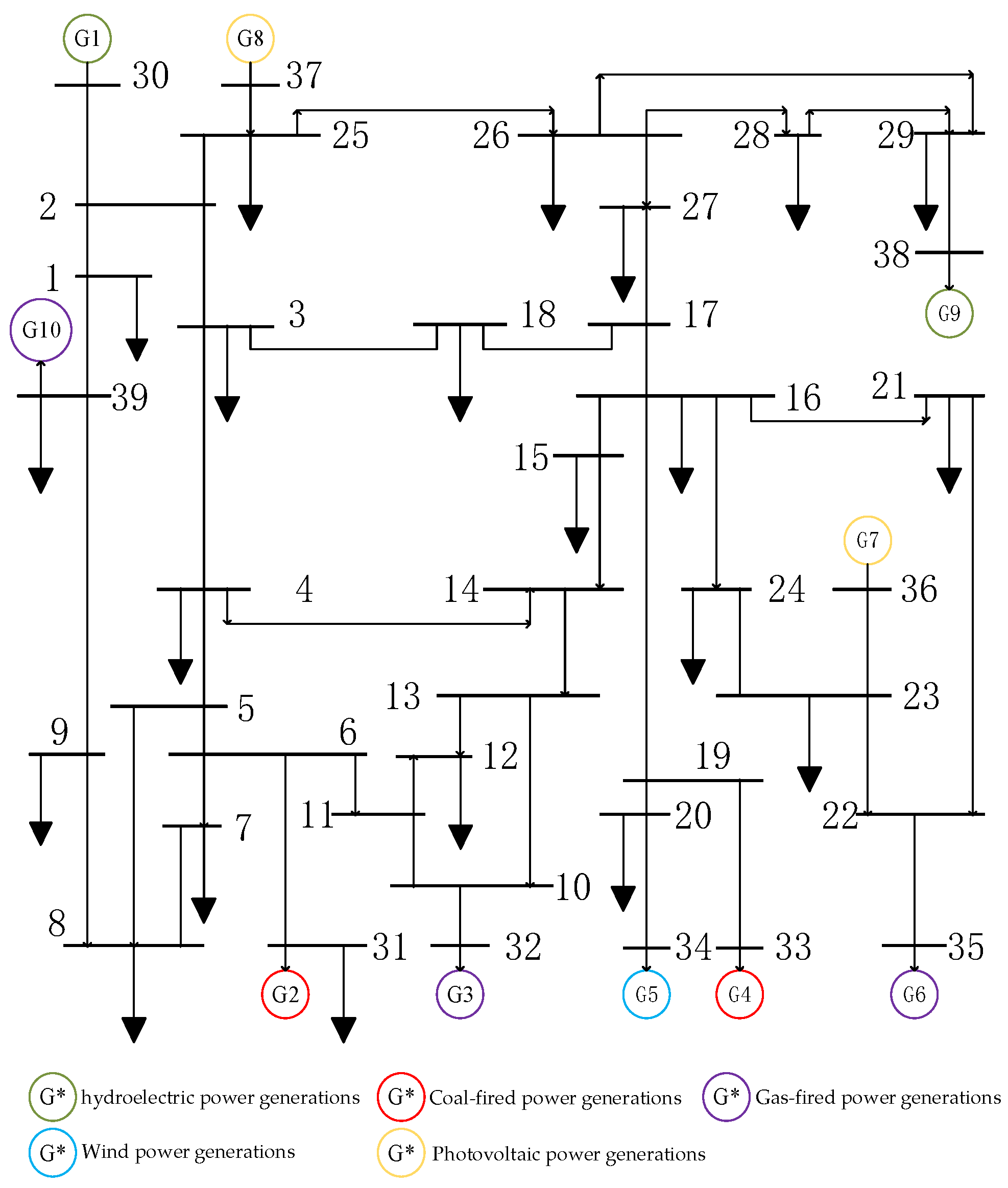
R m = Z m Z m + + Z m

4. Case Studies

4.1. Basic Data

As depicted in Figure 2, this paper validates the proposed method based on a modified IEEE-39 bus system using the Matpower toolbox in MATLAB (MATLAB R2020b). See Table A2 and Table A3 included in Appendix A for the bus and branch data of the system. The modified parameters of each power plant are shown in Table A1 included in Appendix A. The benchmark capacity for power flow calculation is 100 MVA. References [36,37,38,39,40] analyze the power generation types, the expense of power generation is justified, and the carbon intensity of each power plant is given. After the modification, the system contains a total of 10 power plants. Among them, G1 and G9 are hydroelectric power generations, G2 and G4 are coal-fired power generations, G3, G6, and G10 are gas-fired power generations, G5 is wind power generations, and G7 and G8 are photovoltaic power generations. The case of this study is pure fiction.

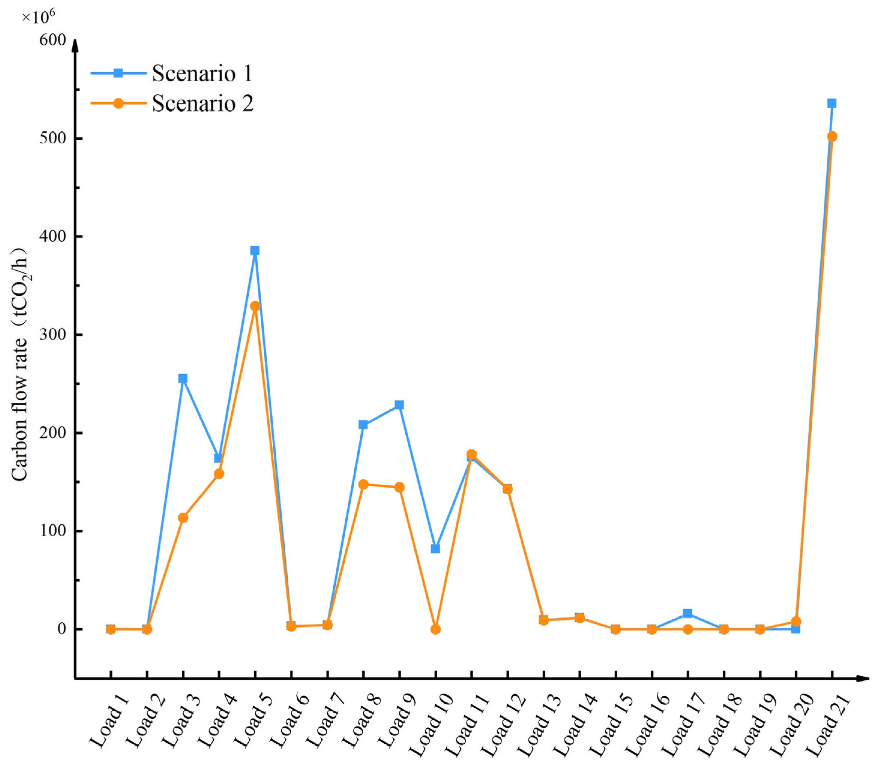
4.2. Example Setting and Analysis

This paper establishes two scenarios to compare and analyze the electricity generation cost, active network loss, and total carbon flow rate of the system. Scenario 1 is employed for calculating the optimal power flow of the traditional power system. Subsequently, the carbon flow distribution of the system is determined by utilizing the optimal power flow distribution and the characteristics of carbon emission flow. Scenario 2 is used to calculate the Pareto optimal frontier of the three objectives (the power generation cost, the active network loss, and the total carbon flow rate of the grid) through the NSGA-III algorithm and determine the optimal solution using the TOPSIS method.
Scenario 1:
Table 1 depicts the optimal power generation from power plant in the IEEE 39-bus system. Under this power plant output scheme, the power generation cost of the grid is 2.3936 million CNY, the active network loss is 37.698 MW, and the total carbon flow rate is 2.25 × 10⁹ tCO2/h.
Scenario 2:
Table 2 depicts the basic parameters of the NSGA-III algorithm in Scenario 2, based on which, the Pareto optimal front is obtained in Figure A6 in Appendix A. The weighting coefficients for the power generation cost, active power loss, and total carbon flow rate are assigned as 0.3, 0.2, and 0.5, respectively, based on which TOPSIS decision method is applied. The first five solutions of the evaluation index are shown in Table 3. The solution with the largest evaluation index is selected as the optimal solution, and the corresponding generator output is shown in Table 4.
Figure 3 depicts the power output from each power plant in Scenario 1 and Scenario 2. Figure 4 and Figure 5, respectively, analyze and compare the node carbon potential and the carbon flow rate of each load in and the two scenarios. It is evident that the carbon potential of each node in Scenario 2 is less than or equal to Scenario 1; the carbon flow rate of each load in Scenario 2 is generally lower compared to Scenario 1. However, the green power cannot meet the demand of some of the loads because some of the green power has been used. Therefore, the carbon flow rate in Scenario 2 surpasses that in Scenario 1.
From Table 1 and Table 4, one can conclude that, compared to Scenario 1, the output of power plants with a high carbon emission intensity in Scenario 2 is significantly reduced. Analyzing the carbon flow rate for each node and load is based on the distribution mechanism and characteristics of carbon emission flow. Considering that the G1, G5, G7, G8, and G9 power plants generate electricity from green energy and have zero carbon emissions, only the carbon flow rate contribution of the G2, G3, G4, G6, and G10 power plants to each node and load is analyzed. The contribution of the power plant to the carbon flow rate of each node and load of the two scenarios are shown in Figure A2, Figure A3, Figure A4 and Figure A5 included in Appendix A. It can be seen that there are more nodes with a distribution of carbon emission flow generated by green power in Scenario 2, which indicates that the renewable resources in Scenario 2 are more fully utilized. In addition, the nodes and final flow load of the carbon emission flow from coal-fired power plants in Scenario 2 are less than in Scenario 1, which indicates a reduction in the output ratio of high-carbon-emitting power plants. From Figure A4 and Figure A5 included in Appendix A, to optimize the carbon emissions of load areas 3, 4, and 5, it is necessary to improve the G2 and G3 power plants; to optimize the load areas of 8, 9, 10, 11, and 12, it is necessary to improve the G4 and G6 power plants; and the load 21 area needs to improve the G10 power plant.
Table 5 compares the power generation cost, real network loss, and total carbon flow rate under the two scenarios. As per the data presented in Table 5, the power generation cost of the system increases by 1.94%, the active network loss increases by 5.78%, and the total carbon flow rate decreases by 20.00%. Compared to Scenario 1, Scenario 2 makes full use of the green power resources in the system and greatly reduces the carbon emissions of the system with a slight increase in power generation costs and active network losses.

5. Conclusions

In pursuit of both economic and environmental considerations within the power system, this paper introduces an optimal power flow model for the power system, factoring in carbon emission intensity and grounded in the principles of carbon emission flow theory. The model optimizes the cost of power generation, active power loss, and total carbon emission rate, and fully mobilizes low-carbon resources to reduce the carbon emissions of the system with consideration for the economy. In addition, the optimal Pareto front is calculated using the NSGA-III multi-objective optimization algorithm, and the optimal output scheme is acquired via the TOPSIS method. This study yields the subsequent conclusions:
  • The numerical simulation results of the IEEE39 bus system show that, with an increase in the economy cost by only 1.94%, the method proposed can reduce carbon emissions by 20.00%.
  • The optimal Pareto front can provide multiple sets of output schemes, which can be more comprehensive and flexible for each scheduling of various resources.
  • The analysis of the carbon flow rate correlation between power plants, nodes, and loads in the power system can also perform small-scale low-carbon optimization on the loads mounted on a node.
The current research does not consider the intermittency and uncertainty of new energy power generation. Next, it is necessary to predict solar and wind energy resources and study the low-carbon optimal scheduling strategy in different periods of the day. At the same time, it can also increase the energy storage equipment for new energy consumption to improve the utilization rate of renewable resources.

Author Contributions

Methodology, G.W.; validation, H.M. and B.W.; formal analysis, F.M.; writing—original draft preparation, G.W.; writing—review and editing, A.M.A. and H.W. All authors have read and agreed to the published version of the manuscript.

Funding

This work is supported by National Natural Science Foundation of China (52167022), Natural Science Foundation of Qinghai (2022-ZJ-935Q).

Institutional Review Board Statement

Not applicable.

Informed Consent Statement

Not applicable.

Data Availability Statement

Data are contained within the article and Appendix A.

Conflicts of Interest

The authors declare no conflict of interest.

Appendix A

Figure A1. Algorithm flow chart.
Sustainability 15 16953 g0a1
Figure A2. Scenario 1: Power plant—node carbon flow rate correlation analysis.
Sustainability 15 16953 g0a2
Figure A3. Scenario 2: Power plant—node carbon flow rate correlation analysis.
Sustainability 15 16953 g0a3
Figure A4. Scenario 1: Power plant—load carbon flow rate correlation analysis.
Sustainability 15 16953 g0a4
Figure A5. Scenario 2: Power plant—load carbon flow rate correlation analysis.
Sustainability 15 16953 g0a5
Figure A6. Pareto Optimal Front.
Sustainability 15 16953 g0a6
Table A1. Modified IEEE-39 Node System Data for Each Power Plant.
BusGeneration TypeActive Output (MW)Reactive Output (MVAr)Power Generation Cost
(Yuan/MWh)
Carbon Intensity
(tCO2/KWh)
MaxMinMaxMin
30Hydroelectric power generation10400400140335.10
31Coal-fired power generation6460300−100260.1856
32Gas-fired power generation7250300150452.0522
33Coal-fired power generation65202500260.1856
34Wind power generation50801670460.10
35Gas-fired power generation6870300−100452.0522
36Photovoltaic power generation58002400387.70
37Photovoltaic power generation56402500387.70
38Hydroelectric power generation8650300−150331.50
39Gas-fired power generation11000300−100452.0522
Table A2. IEEE-39 System Node Data.
BusBus TypeActive Load
(MW)
Reactive Load
(MVAr)
Voltage Amplitude
U m a x (p.u.) U m i n
1PQ BUS97.6044.201.060.94
2PQ BUS0.000.001.060.94
3PQ BUS322.002.401.060.94
4PQ BUS500.00184.001.060.94
5PQ BUS0.000.001.060.94
6PQ BUS0.000.001.060.94
7PQ BUS233.8084.001.060.94
8PQ BUS522.00176.601.060.94
9PQ BUS6.50−66.601.060.94
10PQ BUS0.000.001.060.94
11PQ BUS0.000.001.060.94
12PQ BUS8.5388.001.060.94
13PQ BUS0.000.001.060.94
14PQ BUS0.000.001.060.94
15PQ BUS320.00153.001.060.94
16PQ BUS329.0032.301.060.94
17PQ BUS0.000.001.060.94
18PQ BUS158.0030.001.060.94
19PQ BUS0.000.001.060.94
20PQ BUS680.00103.001.060.94
21PQ BUS274.00115.001.060.94
22PQ BUS0.000.001.060.94
23PQ BUS247.5084.601.060.94
24PQ BUS308.60−92.201.060.94
25PQ BUS224.0047.201.060.94
26PQ BUS139.0017.001.060.94
27PQ BUS281.0075.501.060.94
28PQ BUS206.0027.601.060.94
29PQ BUS283.5026.901.060.94
30PV BUS0.000.001.060.94
31Balance BUS9.204.601.060.94
32PV BUS0.000.001.060.94
33PV BUS0.000.001.060.94
34PV BUS0.000.001.060.94
35PV BUS0.000.001.060.94
36PV BUS0.000.001.060.94
37PV BUS0.000.001.060.94
38PV BUS0.000.001.060.94
39PV BUS1104.00250.001.060.94
Table A3. IEEE-39 System Branch Data.
BranchFromToResistance (p.u.)Reactance (p.u.)Susceptance (p.u.)RatioMax MVA
1123.50 × 10−34.11 × 10−20.69870600
21391.00 × 10−32.50 × 10−20.7501000
3231.30 × 10−31.51 × 10−20.25720500
42257.00 × 10−38.60 × 10−30.1460500
52300.001.81 × 10−201.025900
6341.30 × 10−32.13 × 10−20.22140500
73181.10 × 10−31.33 × 10−20.21380500
8458.00 × 10−41.28 × 10−20.13420600
94148.00 × 10−41.29 × 10−20.13820500
10562.00 × 10−42.60 × 10−30.043401200
11588.00 × 10−41.12 × 10−20.14760900
12676.00 × 10−49.20 × 10−30.1130900
136117.00 × 10−48.20 × 10−30.13890480
146310.002.50 × 10−201.071800
15784.00 × 10−44.60 × 10−30.0780900
16892.30 × 10−33.63 × 10−20.38040900
179391.00 × 10−32.50 × 10−21.20900
1810114.00 × 10−44.30 × 10−30.07290600
1910134.00 × 10−44.30 × 10−30.07290600
2010320.002.00 × 10−201.07900
2112111.60 × 10−34.35 × 10−201.006500
2212131.60 × 10−34.35 × 10−201.006500
2313149.00 × 10−41.01 × 10−20.17230600
2414151.80 × 10−32.17 × 10−20.3660600
2515169.00 × 10−49.40 × 10−30.1710600
2616177.00 × 10−48.90 × 10−30.13420600
2716191.60 × 10−31.95 × 10−20.3040600
2816218.00 × 10−41.35 × 10−20.25480600
2916243.00 × 10−45.90 × 10−30.0680600
3017187.00 × 10−48.20 × 10−30.13190600
3117271.30 × 10−31.73 × 10−20.32160600
3219207.00 × 10−41.38 × 10−201.06900
3319337.00 × 10−41.42 × 10−201.07900
3420349.00 × 10−41.80 × 10−201.009900
3521228.00 × 10−41.40 × 10−20.25650900
3622236.00 × 10−49.60 × 10−30.18460600
3722350.001.43 × 10−201.025900
3823242.20 × 10−33.50 × 10−20.3610600
3923365.00 × 10−42.72 × 10−201900
4025263.20 × 10−33.23 × 10−20.5310600
4125376.00 × 10−42.32 × 10−201.025900
4226271.40 × 10−31.47 × 10−20.23960600
4326284.30 × 10−34.74 × 10−20.78020600
4426295.70 × 10−36.25 × 10−21.0290600
4528291.40 × 10−31.51 × 10−20.2490600
4629388.00 × 10−41.56 × 10−201.0251200

References

  1. Xi, J. Speech at the General Debate of the 75th United Nations General Assembly. People’s Daily, 23 September 2020; edition 003. [Google Scholar] [CrossRef]
  2. Kang, C.; Du, E.; Li, Y.; Zhang, N.; Chen, Q.; Guo, H.; Wang, P. ‘Carbon perspective’ of new power systems: Scientific issues and research framework. Power Syst. Technol. 2022, 46, 821–833. [Google Scholar] [CrossRef]
  3. Tianhua, M.; Qiaoyan, B.; Jun, X.; Deqiang, G. Low-carbon power dispatching and benefit allocation considering carbon emission allowance. Autom. Electr. Power Syst. 2016, 40, 49–55. [Google Scholar]
  4. Hao, X.; Kong, Y. Analysis of the low-carbon transformation path of the power sector under the goal of carbon neutrality. Compr. Util. Resour. China 2022, 40, 179–182. [Google Scholar]
  5. Guo, X.; Lou, S.; Wu, Y.; Wang, Y. Low-carbon Operation of Combined Heat and Power Integrated Plants Based on Solar-assisted Carbon Capture. J. Mod. Power Syst. Clean Energy 2022, 10, 1138–1151. [Google Scholar] [CrossRef]
  6. Liu, H.; Wang, X.; Zuo, D.; Wang, Y. Research on low-carbon transformation of power system under the background of double carbon. Electr. Appl. Ind. 2023, 268, 40–44. [Google Scholar]
  7. Xu, B.; Zhang, G.; Li, K.; Li, B.; Chi, H.; Yao, Y.; Fan, Z. Reactive power optimization of a distribution network with high-penetration of wind and solar renewable energy and electric vehicles. Prot. Control Mod. Power Syst. 2022, 7, 801–813. [Google Scholar] [CrossRef]
  8. Zhang, Y.; Xie, X.; Fu, W.; Chen, X.; Hu, S.; Zhang, L.; Xia, Y. An Optimal Combining Attack Strategy Against Economic Dispatch of Integrated Energy System. IEEE Trans. Circuits Syst. II Express Briefs 2023, 70, 246–250. [Google Scholar] [CrossRef]
  9. Li, K.; Han, X. Distributed algorithm of real-time optimal power flow for distribution network with distributed energy resource. Autom. Electr. Power Syst. 2020, 44, 54–61. [Google Scholar]
  10. Zhang, N.; Zhang, K.; Li, Q.; Liu, J.; Zhao, J.; Sun, G. Optimal power flow calculation of power system containing TCPST based on improved MCCIPM. Electr. Power Eng. Technol. 2021, 40, 144–150. [Google Scholar] [CrossRef]
  11. Zhu, J.P.; Huang, Y.; Ma, L. Assessment on Distributed Generation Accommodation Capability for Distribution Network Based on Uncertain Optimal Power Flow. Autom. Electr. Power Syst. 2022, 46, 46–54. [Google Scholar]
  12. Riaz, M.; Hanif, A.; Masood, H.; Khan, M.A.; Afaq, K.; Kang, B.G.; Nam, Y. An Optimal Power Flow Solution of a System Integrated with Renewable Sources Using a Hybrid Optimizer. Sustainability 2021, 13, 13382. [Google Scholar] [CrossRef]
  13. Wang, C.; Zhu, J.; Li, G.; Zhang, B. Low-Carbon Power Dispatch Based on Evolutionary Algorithm with Adaptive Weight. In Proceedings of the 2011 Asia-Pacific Power and Energy Engineering Conference, Wuhan, China, 25–28 March 2011; pp. 1–4. [Google Scholar] [CrossRef]
  14. Zhang, C.; Yuan, Y.; Zhang, X.; Cao, Y.; Zhang, M. A Day-Ahead Scheduling Planning Model for Wind Power Systems Considering the Impact of Carbon Emission Quotas. Power Syst. Technol. 2014, 38, 2114–2120. [Google Scholar] [CrossRef]
  15. Han, H.; Wei, T.; Wu, C.; Xu, X.; Zang, H.; Sun, G.; Wei, Z. A Low-Carbon Dispatch Strategy for Power Systems Considering Flexible Demand Response and Energy Storage. Front. Energy Res. 2022, 10, 883602. [Google Scholar] [CrossRef]
  16. Li, J.; He, X.; Li, W.; Zhang, M.; Wu, J. Low-carbon optimal learning scheduling of the power system based on carbon capture system and carbon emission flow theory. Electr. Power Syst. Res. 2023, 218, 109215. [Google Scholar] [CrossRef]
  17. Dong, Y.; Shan, X.; Yan, Y.; Leng, X.; Wang, Y. Architecture, Key Technologies and Applications of Load Dispatching in China Power Grid. J. Mod. Power Syst. Clean Energy 2022, 10, 316–327. [Google Scholar] [CrossRef]
  18. Zhong, H.; Zhang, L.; Dong, X. Bi-level emission reduction model of the hybrid power market based on Carbon Emission Flow Theory and source-load coordination. Appl. Sci. 2023, 13, 9100. [Google Scholar] [CrossRef]
  19. Jiang, G.; Wang, B.; Xu, P. A method for power flow calculation and optimal dispatch of gas–thermal–electricity multi energy system considering unit commitment. Energy Rep. 2023, 9, 718–727. [Google Scholar] [CrossRef]
  20. Fakih, S.; Mabrouk, M.T.; Batton-Hubert, M.; Lacarrière, B. Bi-level and multi-objective optimization of renewable energy sources and storage planning to support existing overloaded electricity grids. Energy Rep. 2023, 10, 1450–1466. [Google Scholar] [CrossRef]
  21. Chen, H.; Mao, W.; Zhang, R.; Yu, W. Power System Source-Load Coordinated Low-Carbon Optimal Dispatch Based on Carbon Emission Flow Theory. Power Syst. Prot. Control 2021, 49, 1–11. [Google Scholar] [CrossRef]
  22. Zhou, T.; Kang, C.; Xu, Q.; Chen, Q. Preliminary Theoretical Investigation on Power System Carbon Emission Flow. Autom. Electr. Power Syst. 2012, 36, 38–43+85. [Google Scholar]
  23. Zhou, T.; Kang, C.; Xu, Q.; Chen, Q. Preliminary Investigation on a Method for Carbon Emission Flow Calculation of Power System. Autom. Electr. Power Syst. 2012, 36, 44–49. [Google Scholar]
  24. Li, Y.; Liu, Q.; Zhang, Z.; Liu, J. Calculation method of carbon emission flow based on grid power distribution. Power Grid Technol. 2017, 41, 840–844. [Google Scholar] [CrossRef]
  25. Zhou, T.; Kang, C.; Xu, Q.; Chen, Q.; Xin, J.; Wu, Y. Analysis on Distribution Characteristics and Mechanisms of Carbon Emission Flow in Electric Power Network. Autom. Electr. Power Syst. 2012, 36, 39–44. [Google Scholar]
  26. Cao, D.; Hu, W.; Xu, X.; Wu, Q.; Huang, Q.; Chen, Z.; Blaabjerg, F. Deep reinforcement learning based approach for optimal power flow of distribution networks embedded with renewable energy and storage devices. J. Mod. Power Syst. Clean Energy 2021, 9, 1101–1110. [Google Scholar] [CrossRef]
  27. Yang, N.; Dong, Z.; Wu, L.; Zhang, L.; Shen, X.; Chen, D.; Zhu, B.; Liu, Y. A Comprehensive Review of Security-constrained Unit Commitment. J. Mod. Power Syst. Clean Energy 2022, 10, 562–576. [Google Scholar] [CrossRef]
  28. Nan, Y.; Di, Y.; Zheng, Z.; Jiazhan, C.; Daojun, C.; Xiaoming, W. Research on Modelling and Solution of Stochastic SCUC under AC Power Flow Constraints. IET Gener. Transm. Distrib. 2018, 12, 3618–3625. [Google Scholar] [CrossRef]
  29. Zhu, M.; Xu, C.; Dong, S.; Tang, K.; Gu, C. An integrated multi-energy flow calculation method for electricity-gas-thermal integrated energy systems. Prot. Control Mod. Power Syst. 2021, 6, 65–76. [Google Scholar] [CrossRef]
  30. Yang, N.; Qin, T.; Wu, L.; Huang, Y.; Huang, Y.; Xing, C.; Zhang, L.; Zhu, B. A multi-agent game based joint planning approach for electricity-gas integrated energy systems considering wind power uncertainty. Electr. Power Syst. Res. 2022, 204, 107673. [Google Scholar] [CrossRef]
  31. Deb, K.; Jain, H. An evolutionary many-objective optimization algorithm using reference-point-based nondominated sorting approach, Part I: Solving Problems with Box Constraints. IEEE Trans. Evol. Comput. 2014, 18, 577–601. [Google Scholar] [CrossRef]
  32. Zhang, R.; Feng, X.; Ma, G. Production scheduling and transportation optimization of prefabricated components considering carbon emissions based on NSGA-Ⅲ algorithm. J. Eng. Manag. 2023, 37, 153–158. [Google Scholar] [CrossRef]
  33. Gu, Q.; Luo, J.; Li, X. Multi-objective evolutionary algorithm based on niche. Comput. Eng. Appl. 2023, 59, 126–139. [Google Scholar]
  34. Zhao, Q.; Bai, Q.; Nie, K.; Wang, H.; Zeng, X. Multi-objective optimal allocation of regional water resources based on NSGA-Ⅲ algorithm and TOPSIS decision. J. Drain. Irrig. Mech. Eng. 2022, 40, 1233–1240. [Google Scholar]
  35. Hwang, C.-L.; Lai, Y.-J.; Liu, T.-Y. A new approach for multiple objective decision making. Comput. Oper. Res. 1993, 20, 889–899. [Google Scholar] [CrossRef]
  36. Xu, P.; Fu, W.; Lu, Q.; Zhang, S.; Wang, R.; Meng, J. Stability analysis of hydro-turbine governing system with sloping ceiling tailrace tunnel and upstream surge tank considering nonlinear hydro-turbine characteristics. Renew. Energy 2023, 210, 556–574. [Google Scholar] [CrossRef]
  37. Zhang, Z.; Ban, M.; Guo, D.; Chen, Q.; Jiang, H. A model for Carbon dioxide emission characteristics of coal-fired units for environmental-economic dispatch research. J. Shanghai Jiao Tong Univ. 2021, 55, 1663–1672. [Google Scholar] [CrossRef]
  38. Zhang, S. Research on the Economics of Wind Power Project Investment Based on KWH Cost and Development Potential—Taking Fujian Luoyuan Bay Wind Farm as an Example. China Price Superv. Anti Monop. 2023, 69–72. [Google Scholar]
  39. Li, X.; Gao, Y. Application status and benefit analysis of hub airport PV power generation project. Sol. Energy 2022, 5–11. [Google Scholar] [CrossRef]
  40. Zhang, X.; Liang, J.; Zhao, C. Low-carbon power planning with gas-fired units based on carbon trading. J. Sol. Energy Sin. 2020, 41, 92–98. [Google Scholar]
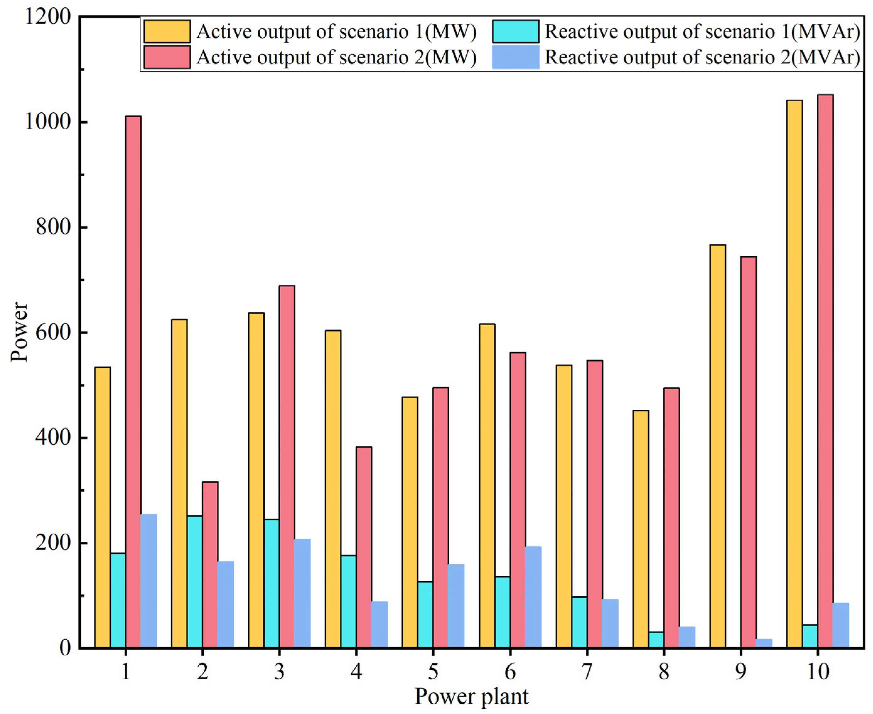
Figure 1. Chart of carbon emission flow in power system. The letter “G” represents the power generation end.
Sustainability 15 16953 g001
Figure 2. Modified IEEE-39 Bus System.
Sustainability 15 16953 g002
Figure 3. Comparative analysis of power plant output in Scenario 1 and Scenario 2.
Sustainability 15 16953 g003
Figure 4. Comparison of node carbon potential in Scenario 1 and Scenario 2. Note: Power injection bus: 30~39; Power consumption bus: 1,3,4,7~9,12,15,16,18,20,21,23~29,31,39.
Sustainability 15 16953 g004
Figure 5. Comparison of load carbon flow rate between Scenario 1 and Scenario 2.
Sustainability 15 16953 g005
Table 1. The output of power plant under Scenario 1.
BusGeneration TypeActive Output (MW)Reactive Output (MVAr)
30Hydroelectric power generation534.00180.64
31Coal-fired power generation624.75251.54
32Gas-fired power generation636.91245.05
33Coal-fired power generation603.75176.16
34Wind power generation477.88126.62
35Gas-fired power generation615.99135.94
36Photovoltaic power generation537.9797.68
37Photovoltaic power generation451.7031.07
38Hydroelectric power generation766.98−6.43
39Gas-fired power generation1041.9944.51
Table 2. Basic parameter setting of NSGA-III Algorithm.
Population SizeMaximum Number
of Iterations
Cross RatioMutation RatioMutation
Probability
2001000.80.20.02
Table 3. The top five individuals in the TOPSIS evaluation index.
OrderPower Generation Cost (Million CNY)Active Network Loss (MW)Total Carbon Flow Rate (×109 tCO2/h)Proximity
Index
12.44039.8781.80070.737
22.45343.5611.71910.7262
32.44342.9701.74900.722
42.43943.3011.74240.728
52.44442.5801.76140.725
Table 4. The output of power plant under Scenario 2.
BusGeneration TypeActive Output (MW)Reactive Output (MVAr)
30Hydroelectric power generation1011.07254.01
31Coal-fired power generation316.35164.31
32Gas-fired power generation688.86206.66
33Coal-fired power generation382.4087.54
34Wind power generation495.57158.96
35Gas-fired power generation561.94192.43
36Photovoltaic power generation546.9292.45
37Photovoltaic power generation494.4939.83
38Hydroelectric power generation744.3516.54
39Gas-fired power generation1052.1685.70
Table 5. Comparison of the optimization results of Scenario 1 and Scenario 2.
ScenarioPower Generation Cost
(Million CNY)
Active Network Loss (MW)Total Carbon Flow Rate (×109 tCO2/h)
12.393637.6982.25 × 109
22.440039.8781.80 × 109
Disclaimer/Publisher’s Note: The statements, opinions and data contained in all publications are solely those of the individual author(s) and contributor(s) and not of MDPI and/or the editor(s). MDPI and/or the editor(s) disclaim responsibility for any injury to people or property resulting from any ideas, methods, instructions or products referred to in the content.

