Abstract
Short-term load forecasting is a prerequisite for achieving intra-day energy management and optimal scheduling in integrated energy systems. Its prediction accuracy directly affects the stability and economy of the system during operation. To improve the accuracy of short-term load forecasting, this paper proposes a multi-load forecasting method for integrated energy systems based on the Isolation Forest and dynamic orbit algorithm. First, a high-dimensional data matrix is constructed using the sliding window technique and the outliers in the high-dimensional data matrix are identified using Isolation Forest. Next, the hidden abnormal data within the time series are analyzed and repaired using the dynamic orbit algorithm. Then, the correlation analysis of the multivariate load and its weather data is carried out by the AR method and MIC method, and the high-dimensional feature matrix is constructed. Finally, the prediction values of the multi-load are generated based on the TCN-MMoL multi-task training network. Simulation analysis is conducted using the load data from a specific integrated energy system. The results demonstrate the proposed model’s ability to significantly improve load forecasting accuracy, thereby validating the correctness and effectiveness of this forecasting approach.
1. Introduction
Environmental pollution and energy shortages continue to constrain the sustainable development of human society. A new energy revolution has been launched globally, driven by China’s national strategic goal of achieving carbon peak by 2030 and carbon neutrality by 2060. It is necessary to integrate this energy revolution with the advances of the digital revolution [1,2,3,4]. How to achieve efficient and cost-effective interconnection in different energy sectors, strengthen energy collaboration, and improve energy efficiency has become a prominent issue of widespread concern in the industry [5,6,7,8]. To meet the urgent need for complementary and coordinated operation across various energy types, the Integrated Energy System (IES) [9,10] emerged. Short-term load forecasting serves as a prerequisite for intra-day energy management and optimal scheduling in IES, and its prediction accuracy directly influences the stability and economy of the system during operation.
The prediction of loads in integrated energy systems involves four key aspects: data preprocessing, model selection, optimization strategies, and algorithm selection. Over the years, extensive research has been conducted in the field of short-term load forecasting methods for integrated energy systems, leading to significant achievements [11,12,13]. Existing forecasting methods mainly include traditional machine learning, ensemble learning, deep learning, reinforcement learning, and transfer learning [14,15]. Ping et al. [16] predicted the wind speed based on the wavelet neural network model and solved the problem of low prediction accuracy caused by slow convergence speed. Shi et al. [17] considered the coupling relationship among thermal, electric, and gas loads in the industry. By analyzing multiple data, such as weather information and historical data, the authors explored the coupled relationship between the data. A prediction method based on deep learning and multi-task learning was proposed to enhance the model’s predictive ability and obtain more accurate results. Wang et al. [18] considered the high-dimensional temporal dynamics and proposed an encoder-decoder model based on a Long Short-Term Memory (LSTM) network. In this work, the effectiveness of deep learning methods in integrated energy load forecasting is validated. Reference [19] proposes a new dynamic multi-sequence intelligent data-driven decision-making method by combining SCUC decision-making with dynamic multi-sequence models. Tan et al. [20] analyzed the coupling relationship between different subsystems and proposed a joint prediction method for electric, heating, cooling, and gas loads based on multi-task learning and least squares support vector machines (LS-SVM). In the work of Zhou et al. [21], a comprehensive load forecasting model based on the Bi-Directional Generative Adversarial Network (BiGAN), data augmentation, and transfer learning techniques is proposed. The Zhou et al. model considers the issue of data scarcity in information systems. While maintaining a high level of predictive accuracy, the authors address the challenges that arise when incorporating new users into integrated energy systems. Their proposal also enhances the robustness of the integrated energy system and expands its generality.
Recently, with the emergence of various intelligent systems and the integration of distributed energy resources, the energy interaction structure has become more diverse [22]. Consequently, the energy consumption patterns of users under different structures have become increasingly real-time and complex [23,24]. In the actual operation process, the application scenarios in the integrated energy system may change (e.g., the start of lengthy school breaks or the hosting of large-scale events requiring accommodation of a large influx of visitors), there may be equipment failures and other extreme conditions, and the load data that occurs at this time is unconventional data. In these cases, the resulting load data can be classified as unconventional. Due to the scarcity of data on unconventional patterns, parameter optimization becomes challenging, especially considering the sensitivity of neural networks to abnormal data. The predictive accuracy of neural networks significantly decreases when the load is influenced by complex factors and exhibits strong randomness and nonstationary characteristics. So far, researchers have mostly focused on conventional design aspects—such as model selection, optimization strategies, and algorithm choices—for integrated energy systems, which are insufficient to meet the operational requirements of diverse patterns and volatile operating conditions. Based on these considerations, on one hand, it is necessary to design the data feature preprocessing stage to eliminate abnormal data. Moreover, to meet the requirements of real operating conditions, the influence of event-driven factors should be taken into account, and an analysis of users’ historical energy consumption patterns should be conducted to enhance the overall stability of the system. On the other hand, appropriate parameters should be selected in the stages of model selection, optimization strategies, and algorithm choices. By incorporating these aspects into the design process, the accuracy of load forecasting under normal patterns can be improved.
Currently, there is continuous development of methods for identifying anomalies in time series data. Common cleansing methods [25] include statistical approaches such as the Gaussian distribution, box plots, and clustering methods used in machine learning. Based on the assessment of whether the measurement data errors follow a zero-mean Gaussian distribution, the “3σ rule” [26] is employed to detect outliers. Although this method is simple and convenient, it is influenced by various factors during the operation of an integrated energy system. The output data from the system exhibits multidimensionality, randomness, intermittency, and uncertainty [27,28,29]. The above-mentioned methods greatly reduce the accuracy of identifying abnormal data and can only detect simple outliers. Although clustering algorithms [30] are machine learning techniques capable of detecting most outliers, they struggle to identify anomalies hidden within sequences, failing to meet the requirements for data analysis quality. In summary, there is an urgent need for a method which can eliminate the presence of abnormal data in time series under normal data patterns that is applicable for multi-load forecasting in integrated energy systems.
To address this gap in the research, this paper proposes a comprehensive multi-load forecasting approach for integrated energy systems based on the Isolation Forest algorithm and dynamic orbit method. In this study, the contributions of this paper can be summarized as follows:
- A new anomaly data detection method is proposed. Based on the iForest algorithm, the extreme values and some outliers of the high-dimensional data matrix are identified.
- A new abnormal data correction method is proposed. The dynamic orbit method is used to analyze and repair the abnormal data hidden in the time series. If the abnormal value data are found, the system triggers an alarm, enters the behavior analysis link of the news surface, visualizes the separation window, and distinguishes the type of abnormal value.
- To determine the dependencies between multiple loads. The correlation analysis of the multivariate load and its weather data is carried out by an autoregressive (AR) method and maximal information coefficient (MIC) method, and a high-dimensional feature matrix is constructed.
- A new load forecasting structure is proposed. Based on the TCN-MMoL (multi-gate mixture-of-experts of LSTM) multi-task training network, the predicted value of the multi-load is output.
2. Related Work
2.1. The Isolation Forest
The Isolation Forest (iForest) [31,32,33] is a nonparametric anomaly detection algorithm that does not require specifying a specific physical model or labeling the anomalous data. It can be used to identify outlier points in a dataset. It estimates the degree of isolation of data points by means of binary tree, so as to determine whether it is an abnormal point.
The core idea of the Isolation Forest is to utilize the isolation of data points in the feature space to detect anomalies. It assumes that normal data points are relatively dense in the feature space, while anomalies are relatively few and more isolated. Therefore, anomalies should be separated more quickly by the Isolation Forest model. Typically, the basic steps of the Isolation Forest algorithm are as follows:
- Randomly select a feature and choose a split point within the range of the feature values.
- Use the selected feature and split point as the splitting rule to divide the data points into two subsets.
- Recursively repeat steps one and two until each subset contains only one data point or reaches the maximum depth defined in advance for the tree.
- Construct multiple random trees and form a random forest.
- For each data point, calculate its path length in the random forest, which is the average number of edges from the root node to the data point.
- The anomaly score of a data point is measured by its path length. A shorter path length indicates an outlier that is easily isolated, while a longer path length indicates a normal point.
- Finally, by setting a threshold, the path lengths can be compared with the probability of abnormal points to determine which data points should be classified as anomalies.
The Isolation Forest algorithm utilizes binary trees to partition the data, and the depth at which a data point lies in the binary tree reflects its level of “isolation” [34]. The decision-making process of the algorithm is illustrated by Figure 1.
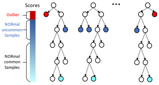
Figure 1.
Isolation Forest Decision Diagram.
The Isolation Forest algorithm exhibits excellent scalability and efficiency in anomaly detection and also demonstrates good performance for high-dimensional and large-scale datasets. Serving as an ensemble-based, fast, and unsupervised anomaly detection method, the Isolation Forest algorithm achieves high efficiency and accuracy, delivering promising results in the field of industrial inspection [35].
2.2. Dynamic Orbit
For anomaly detection in time series data, the common approach is to set a threshold value, and when data exceeds this range, it is considered anomalous. However, due to the strong volatility and randomness of multiple load fluctuations within an integrated energy system, the conventional time series anomaly detection methods are not suitable for the application scenarios of such systems. Hence, this study proposes a dynamic orbit approach specifically designed for anomaly repair in integrated energy system data.
The dynamic orbit consists of a middle orbit, an upper orbit, and a lower orbit, as illustrated in Figure 2. The dynamic orbit takes the form of a channel, where data values within the channel range are considered normal, while data values that cross the channel and fall outside of it are classified as anomalies.
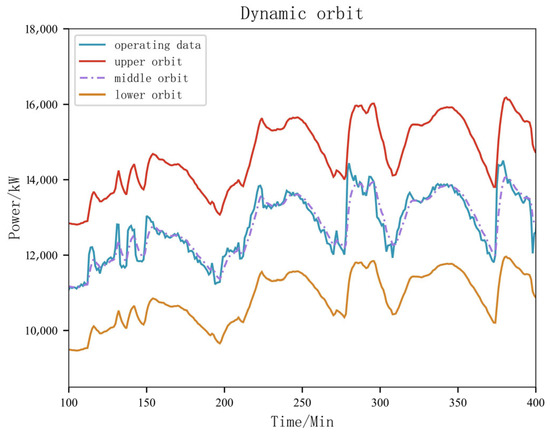
Figure 2.
Schematic Diagram of Dynamic Orbit.
The calculation of the dynamic orbit primarily involves two major steps. First, the establishment of the reference orbit of the dynamic orbit is achieved using the moving average method. The concept of the reference orbit is derived from the smoothing method [36], which is commonly used for trend analysis and prediction; the smoothing techniques reduce the influence of short-term random fluctuations on a sequence and thus achieve a smoother sequence. Depending on the specific smoothing technique employed, it can be categorized into the simple moving average method, exponential moving average method, and weighted moving average method.
Next, calculations are performed for the upper and lower bound orbits. After determining the reference orbit, calculations are performed for the upper and lower bound orbits using the following specific formulas shown in Equations (1) and (2):
In Equations (1) and (2), UO is the abbreviation of the upper orbit, MO is the abbreviation of the middle orbit, and LO is the abbreviation of the lower orbit. M1 represents the margin of the upper orbit, and M2 represents the margin of the lower orbit.
Simple Moving Average
The simple moving average (SMA) method [37] gradually moves along the time series and calculates the sequential average over a certain number of terms to reflect the long-term trend of the sequence. The SMA is obtained by summing the previous historical data points in the time series and calculating their arithmetic mean. As shown in Equation (3), when the time window scale is represented by l, the SMA index at the t time node can be calculated as:
where represents the data at the t time node.
The SMA indicator effectively mitigates the rapid fluctuations in the time series by summing and averaging the values, resulting in smoother peaks and valleys. However, this calculation method assigns equal weight to the time series data, disregarding the varying importance of data at different time points. As a result, it exhibits insensitivity to changes in the time series and possesses a certain degree of lag.
The exponential moving average (EMA) [38] addresses several issues associated with SMA, including the fact that SMA assigns equal weight to all data points in a time series. In contrast, EMA assigns different weight to the data points at each time point in the time series. This is based on the assumption of recent bias, which posits that there is a strong correlation between the future trend of a time series and its recent volatility. EMA accomplishes this by applying exponential decay to the weight of the time series data. It gives greater weight to the most recent data points over past data points. Equation (4) provides a recursive calculation for EMA:
where β represents the degree of weight reduction. Through this approach, the EMA indicator can effectively filter out noise that is less correlated with changes in the time series trend and become more sensitive to the variations in the time series. As a result, the prediction of time series trends becomes more reliable and accurate.
The weighted moving average (WMA) [39], which is similar to the EMA indicator, allocates greater weight to recent data in a time series. The specific calculation method for WMA is as follows:
where denotes the predefined weights.
In this paper, we employ the WMA indicator. Starting from the first data point in the time series, the weights assigned to the time series data increase linearly as the time series expands.
2.3. Temporal Convolutional Neural Network
Temporal convolutional neural network (TCN) [40] is a deep learning model used for handling time series data. It consists of causal convolution, dilated convolution, and residual connections, as illustrated in Figure 3. TCN exhibits the following characteristics when dealing with time series data.
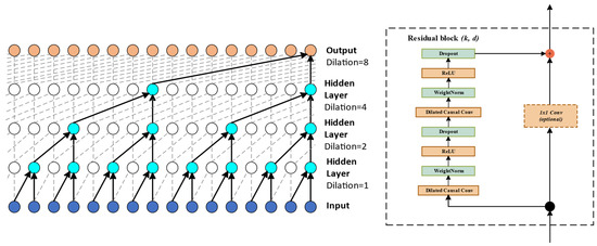
Figure 3.
TCN Network Layer.
- Causal Convolution: TCN utilizes a unique form of causal convolution, which preserves the causality of the input sequence, prevents leakage of future data, and expands the receptive field. The entire network’s perception range and information length are the same as the input sequence, ensuring that the sequence influences the deep network as a whole.
- Dilated Convolution: To address the problem of information overlap, TCN employs dilated convolution. Unlike regular convolution, the convolutional kernel of dilated convolution reads data through interval sampling. This sampling technique allows TCN to acquire a larger receptive field for sequence feature extraction and preserve more historical information. The output of dilated convolution is obtained by accumulating the element-wise multiplication of the convolutional kernel and the input.
- Residual Module: To address the problem of gradient vanishing caused by convolutional degradation, TCN introduces the residual module, which consists of two dilated causal convolutions, batch normalization, dropout, and ReLU activation function, among others. The advantage of the residual module is that it prevents excessive information loss during feature extraction. By adding the features extracted to the input data using causal convolutions, the final output is obtained. Additionally, a 1 × 1 convolutional layer is added to maintain the same scale of output as the input.
Compared to traditional recurrent neural networks (RNN), TCN utilizes convolutional operations to capture the local dependencies in time series data, resulting in higher parallelism and greater computational efficiency. With causal and dilated convolutions, TCN is able to process long input sequences by rapidly reading them as a whole. The backpropagation path is different from the time direction of the sequence, which prevents the issues of gradient explosion and gradient vanishing.
2.4. Long Short-Term Memory
Long Short-Term Memory (LSTM) [41] is a variant of recurrent neural networks (RNN) that effectively handles long-term dependencies in sequential data. At the core of LSTM is a structure called the memory cell, which stores and updates information in the sequence. LSTM comprises three gate structures—the input gate, forget gate, and output gate—which control the flow of information within the memory cell. The input gate determines how the current input and previous hidden state affect the state of the memory cell. The forget gate determines what information in the memory cell should be discarded, and the output gate determines how the state of the memory cell influences the current hidden state and output. Through this mechanism, LSTM can learn and extract long-term dependencies in sequences while avoiding the issues of vanishing or exploding gradients. The LSTM structure is illustrated in Figure 4.
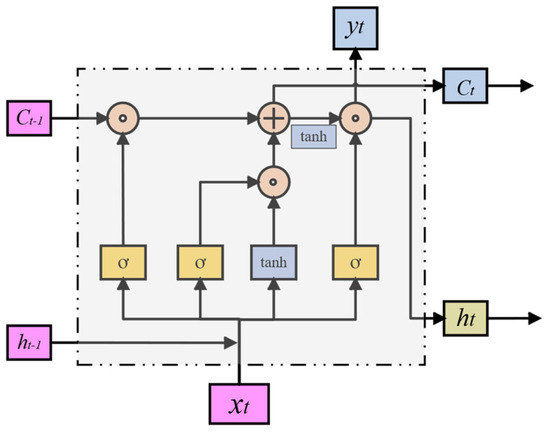
Figure 4.
Schematic of LSTM.
2.5. The Multi-Task Learning Mechanism
The multi-task learning mechanism [42,43] involves simultaneously learning multiple related subtasks within a learning framework, which enables the sharing of learned information throughout the learning process. Compared to single-task learning, multi-task learning is able to better extract the coupling relationships that exist among multiple tasks. This avoids the handling of complex real-world problems, such as independent subtasks in single-task learning, followed by merging and superimposing the results, which neglects the rich information pertaining to the relationships between subtasks. Figure 5 illustrates the principles of a single-task versus a multi-task learning mechanism.
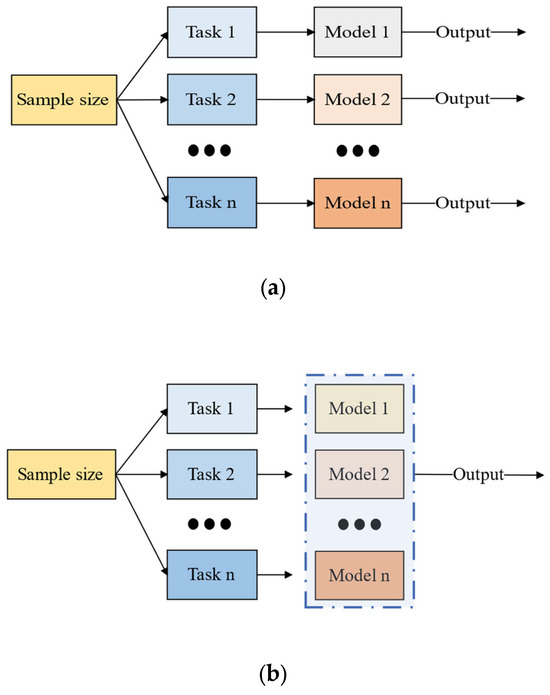
Figure 5.
Single-Task vs. Multi-Task Learning Schematic. (a) Single-task learning. (b) Multi-task learning.
Multi-task learning can be divided into two types of sharing mechanisms: hard sharing and soft sharing [44]. In the hard sharing mechanism, the stronger the correlation between subtasks, the better the training effect of the model. However, if there is poor correlation among some subtasks, the training effect of the model will be unsatisfactory. The traditional approach to multi-task learning usually adopts the hard sharing mechanism, which consists of a parameter-sharing layer and subtask-learning layers. The parameter-sharing layer receives all feature data extracted in the early stages and processes them in the sharing layer. Then, the subtask layers selectively train corresponding feature data based on their own requirements and finally output prediction results.
Traditional multi-task learning typically also adopts parameter sharing, where all subtasks use the same feature extraction layer for feature extraction. However, such methods overlook diversity among subtasks, thereby restricting the expressive capacity of the model.
To address this issue, Google proposed the MMoE model [45] that possesses a different core mechanism compared to the traditional hard sharing approach, which forces all subtasks to share the same feature extraction layer. Instead, in MMoE, the feature extraction layer is divided into multiple experts according to certain rules, and a gating mechanism is introduced to control the weight of each expert for each subtask. Each subtask has an independent gating network which allows each subtask to retain its own diversity while sharing relevant information through training. For task k, the model is calculated as follows:
In Equations (6) and (7), n represents the number of expert networks, m represents the number of subtasks, signifies the proportion of weight for the ith expert network in the mth subtask, and represents the output of the ith expert network.
3. Data Feature Preprocessing
To date, scholars have extensively researched and achieved substantial results in the comprehensive energy system under conventional models [46,47,48,49]. However, most studies focus primarily on model parameter design in the prediction model stage. Currently, there is a lack of literature that conducts in-depth analysis and processing of historical data in the feature preprocessing stage. Historically, there have been issues such as missing data and transmission errors during the communication process, as well as deviations from historical data trends due to special events. The anomalies and missing data resulting from these issues undoubtedly have a significant impact on the accuracy of short-term load forecasting models for integrated energy systems. Therefore, this study employs the iForest and dynamic trajectory methods to analyze and eliminate the abnormal data, as shown in Figure 6. Subsequently, the missing values are filled in for both the eliminated missing data and the original missing data. The data feature preprocessing flowchart is depicted in Figure 6, which illustrates the specific steps taken.
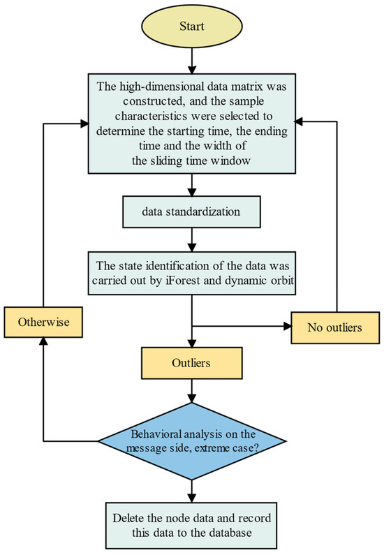
Figure 6.
Data Feature Preprocessing.
The first step involves constructing a high-dimensional data matrix. The separation window technique is used to construct the matrix, incorporating n-dimensional features, such as cooling load, heating load, electric load, and weather data.
In the second step, data standardization is applied. This procedure ensures consistent measurement standards, eliminates biases and outliers, enhances data quality and reliability, and improves the computational efficiency of the network.
Lastly, the identification and repair of data outliers in the high-dimensional data matrix are performed using the iForest method and the dynamic trajectory method. Any detected outliers trigger an analysis of behavioral patterns, helping to determine if they are extreme events. If they are so identified, they are recorded in the database to assist in the development of integrated prediction algorithms.
3.1. Construction of High-Dimensional Data Matrices
The first step in data feature preprocessing is to construct an appropriate high-dimensional data matrix, denoted as . In this study, the data elements of n-dimensional nodes are sampled. At a specific sampling time t, the n-dimensional sampling nodes can be arranged into a column vector, as shown in Equation (8):
As the sampling time increases, the number of column vector data also increases. Therefore, a time series can be constructed, as follows:
To meet the requirements of real-time computation, the collected data are analyzed by using a sliding time window. The width of the sliding time window is set as τ, which includes the data collected at time t and the historical data from t-τ to t. The high-dimensional data matrix is then constructed using all the data within this time window, as shown below:
where τ represents the time window.
The selection of the time window should meet the following criteria: it should be of appropriate width to meet the needs of real-time detection while also including all the measured data from each partition.
3.2. Data Standardization
Construction of the high-dimensional data matrix . All of the data undergo standardization processing, including dimensionless transformation and normalization [50]. After processing, different data will be transformed into the same measurement standard, facilitating comparison and analysis. Standardization operations can eliminate bias and outliers in the data, improve data quality and reliability, and reduce data dimensionality, leading to a reduction in computation time and complexity.
3.3. Data Outlier Recognition and Correction
Due to fluctuations in load and other factors, the operational process of the integrated energy system is inherently a dynamic and variable process. After obtaining a multidimensional data matrix composed of cooling load, heating load, electric load, meteorological data, and other data, the first step is to remove outliers in the data using the iForest algorithm. Then, using the dynamic trajectory method, abnormal values within the time series are removed and repaired. When an exceptional value exceeds the upper bound of the dynamic trajectory, the corresponding value in the multidimensional data matrix is assigned as the baseline value. When an exceptional value exceeds the lower bound of the dynamic trajectory, the baseline value is assigned as the corresponding value in the multidimensional data matrix. The dynamic trajectory acts as a highway, ensuring that data operates within a normal range. Simultaneously, in the event of an abnormal alert, the system triggers the behavioral analysis function of the message interface. The system analyzes the activities within the system to determine whether the abnormality is due to a sudden event, such as a large-scale activity or the deployment of new buildings and their equipment. This analysis provides valuable experience for future production and daily life and aids in the development of integrated prediction algorithms.
4. Construction of Input Feature Set and Multi-Load Prediction Model
4.1. Correlation Analysis of Multi-Loads
The integrated energy system is a complex system composed of the core components of the cooling system, heating system, and electric energy system, as well as various information systems including meteorological and economic systems. As an information-intensive, immense, and dynamic system, it involves the mutual coupling and synergistic complementarity of multiple energy sources. Furthermore, with the continuous expansion and increasing complexity of the integrated energy system, detection and measurement technologies have been continuously developing. Various measurement systems and devices are being applied, leading to exponential growth in the related data [51].
Faced with the increasing temporal dimension of operational data in the integrated energy system, a massive amount of data has been generated with both temporal and spatial characteristics. Analyzing the collected high-dimensional feature data aids in gaining a general understanding of the entire integrated energy system and provides qualitative guidance for the construction of prediction models in terms of direction and scope.
4.1.1. Autoregressive System Analysis
In this study, an autoregressive model (AR model) [52,53] is employed to analyze the temporal state characteristics of short-term time series and provide a basis for determining the moving average period, l, in the dynamic track method. The autoregressive model uses its own past values as regression variables, describing the linear regression relationship of a random variable at a future moment based on a linear combination of its previous values. Consider a time series that satisfies the following equation:
where are coefficients, and represents the white noise value.
The temporal state characteristics of the load data are analyzed based on the autocorrelation coefficient function (ACF) and the partial autocorrelation coefficient function (PACF) of the AR model. Due to the limitation of the length of the article, the cooling load data, heating load data, and electric load data are taken as examples. As shown in Figure 7, the cooling load autocorrelation coefficient analysis diagram and the partial autocorrelation coefficient analysis diagram are shown. As shown in Figure 8, the heating load autocorrelation coefficient analysis diagram and the partial autocorrelation coefficient analysis diagram are shown. As shown in Figure 9, the electric load autocorrelation coefficient analysis diagram and the partial autocorrelation coefficient analysis diagram are shown.
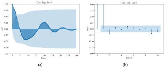
Figure 7.
Analysis Diagram of Cooling Load. (a) ACF. (b) PACF.
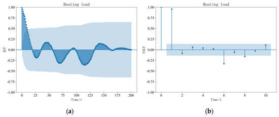
Figure 8.
Analysis Diagram of Heating Load. (a) ACF. (b) PACF.
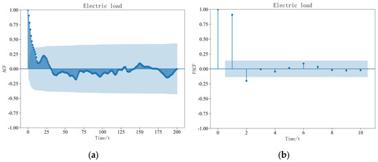
Figure 9.
Analysis Diagram of Electric Load. (a) ACF. (b) PACF.
According to Figure 7, Figure 8 and Figure 9, the blue regions represent the confidence intervals of the correlation coefficient plots. In this study, we chose a confidence level of 95% and a time granularity of 15 min. From the autocorrelation coefficient plot of the cooling load, we can observe a strong coupling relationship between the load sequences in shorter time intervals. Specifically, at a lag time of 13 intervals, the positive autocorrelation coefficients of the cooling load remain above 0.5. Similar analyses of the autocorrelation coefficients of the heating load and electric load reveal that the positive autocorrelation coefficients of the heating load decrease below 0.5 after the fourth value, and the positive autocorrelation coefficients of the electric load also decrease below 0.5 after the fourth value. This indicates that the mutual coupling effect between cooling loads is stronger as compared to that of the heating and electric loads.
Furthermore, by observing the autocorrelation coefficients of the cooling load, heating load, and electric load, we find that each exhibits certain periodic variations. Moreover, compared to the electric load, the cyclic variations of the cooling load and heating load are more pronounced and organized. By examining the partial autocorrelation coefficients of the cooling load, heating load, and electric load, we can conclude that there exists a direct and strong coupling relationship between the loads within the first three time intervals.
4.1.2. Maximal Information Coefficient Analysis
Pearson correlation coefficient or Spearman correlation coefficient can be effectively used to measure the linear correlation between data, and even to determine the mathematical formulas for linear or simple nonlinear relationships through regression analysis. However, in integrated energy systems, the coupling relationships between multiple systems are complex, and there exists not only linear relationships but also a significant number of nonlinear relationships between the data. Nonlinear relationships cannot be simply expressed using mathematical formulas.
The maximal information coefficient (MIC) method [54,55] can measure the strength of both linear and nonlinear associations between data, allowing for the discovery of diverse types of relationships among different types of load data. Therefore, in this study, the MIC is used to analyze the spatiotemporal characteristics of multiple systems and to construct a high-dimensional feature matrix for model inputs. Figure 10 presents the MIC heatmaps for various systems, including the electric energy system, cooling system, heating system, and weather system.
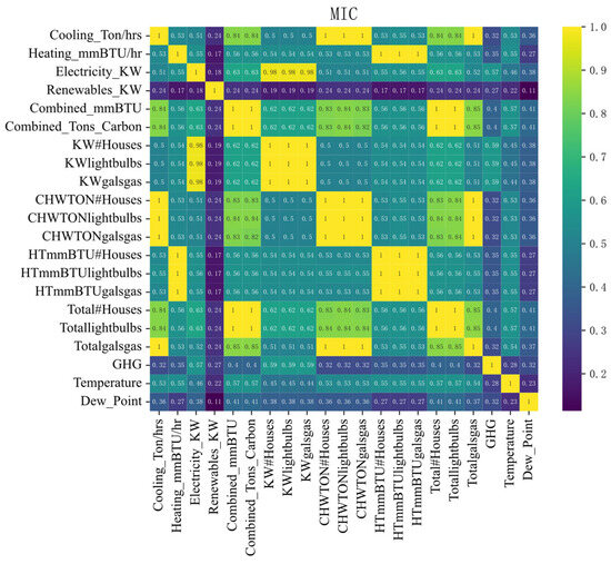
Figure 10.
MIC Heat Map of Characteristic Sequence.
The legend on the right side of Figure 10 represents the correlation levels between the major features, with values ranging from 0 to 1. A value below 0.3 indicates weak correlation between the two features, while a value above 0.7 indicates strong correlation between them.
As shown in the figure, the cooling system, heating system, and electric system serve as the three major foundational systems in integrated energy systems. The correlation coefficient between the cooling load and heating load is 0.57, indicating a strong correlation and a close coupling relationship between the cooling and heating systems. The correlation coefficient between the cooling load and electric load is 0.7, suggesting a particularly tight connection between the cooling and electric systems in the production and daily life of integrated energy systems.
The correlation coefficient between the heating system and the electric system is 0.48, indicating a coupling relationship between the two in the integrated energy system, although it is relatively weaker than the cooling-electric system relationship. In addition, it can be observed that the cooling, heating, and electric systems also exhibit a close correlation with temperature and dew point. Furthermore, there is a strong correlation between the building usage of each system and its respective systems.
4.2. Construction of Input Feature Set
Based on the analysis of MIC data, this study selects eight characteristic variables as inputs in order to construct the input feature set, which include cooling load, heating load, electric load, temperature, dew point, and the number of buildings using cooling, heating, and electric loads. The specific list of these variables is presented in Table 1.

Table 1.
Input List of Feature Sets.
4.3. Multi-Load Prediction Model
4.3.1. Model Framework
In this study, a multi-task learning framework called the TCN-MMoL (referred to as the CMMoL model) is utilized to establish a multi-load prediction model, as illustrated in Figure 11. First, when the network model receives the input high-dimensional feature matrix, the TCN network is employed to explore and extract the temporal and spatiotemporal characteristics of the high-dimensional data features. Subsequently, the TCN network feeds the learned feature information into the preceding LSTM network in the expert layer, further refining the feature matrix. The unique memory capability of the LSTM units is utilized to extract temporal dependencies within the feature matrix. Lastly, the processed data features are input into the multi-gate network model, where the expert network layer and its distinct gating mechanism predict and output power values for cooling load, heating load, and electric load.
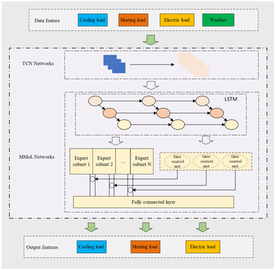
Figure 11.
Model Framework.
4.3.2. Evaluation Metrics
In this study, the mean absolute percentage error (MAPE) is adopted as the primary evaluation metric for the predictive performance of each model, with the mean absolute error (MAE) selected as a secondary evaluation metric. The calculation formulas for MAPE and MAE are as follows:
In Equations (12) and (13), represents the actual power load data, represents the predicted power load data, and n represents the sample size of the power load data.
5. Experiment Analysis
5.1. Experiment Description
In this paper, experiments are carried out on the hardware platform of Xeon4213R CPU and NVIDIA RTX 3080 GPU. The TensorFlow and Keras deep learning frameworks are built and implemented in the Python programming language.
The load data of the example are derived from the IES cooling, heating, and electric load data and other characteristic data of the Tempe campus of Arizona State University from 1 January 2022 to 1 May 2023. The sampling granularity is 15 min. The load data are derived from the project network database of the campus. The campus has 288 buildings and more than 50,000 teachers and students. It also has CCHP (Combined Cooling, Heating, and Power), electric boilers, gas boilers, and power-to-gas P2G (Power-to-Gas) and other energy conversion equipment. The meteorological data comes from the public meteorological data for the corresponding time period on the meteorological website. In the division of the dataset, 75% is taken as the training set, 15% as the verification set, and 10% as the test set.
5.2. Analysis of the Necessity of Global Use of the iForest Algorithm
Among the instance data selected in this paper, there are 22 statistical features and more than 46,000 running data. In the face of massive experimental data, this paper uses the iForest algorithm to process global data. The algorithm has the characteristics of high processing accuracy and fast calculation speed and is suitable for dealing with outliers in big data [56]. At the same time, the processed data are more conducive to the implementation of the dynamic orbit method.
Due to the limited space, only the electric load data are taken as an example to show the processing process and analyze the necessity. Figure 12 shows the historical data running diagram of the electric load before processing.
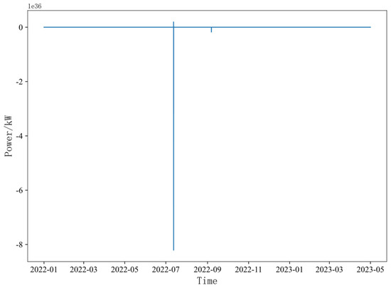
Figure 12.
Electric Load Running Diagram Before Processing.
Through observation, extreme value points are found in the data, which makes the dynamic power load data present as a straight line; there is also an order of magnitude difference between the extreme value points and the normal data.
In order to express this order-of-magnitude relationship more clearly, the contour distribution map of the electric load is drawn. As shown in Figure 13, the white points in the figure are normal values and are distributed in the contour distribution cluster of the blue area. The closer to the center, the darker the color; the more inclined to the outside of the contour, the lighter the color. The black dots in the figure are outliers, which are scattered in the dark green area.
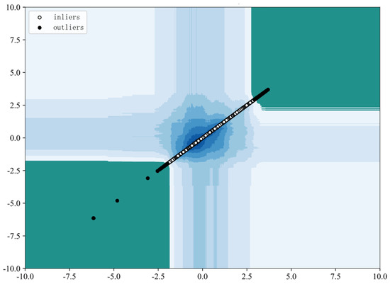
Figure 13.
Electric Load iForest Contour Map.
By detecting and eliminating the abnormal points, the actual operation data of the power load after elimination are shown in Figure 14. By comparing the operation charts before and after the power load preprocessing, it can be seen that the outliers in the data have been eliminated, and the power load operation data show a trend and regularity, indicating that the method can efficiently process the outliers in the data.
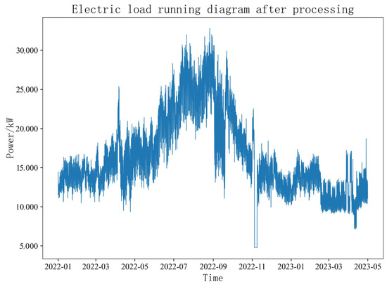
Figure 14.
Electric Load Running Diagram After Processing.
5.3. Super Parameter Settings
In the data feature preprocessing and network model, there are hyperparameters in the upper and lower margin values of dynamic orbits, the TCN network layer, and the MMoL network layer. According to the learning effect of model training, the control variable method is used to determine the hyperparameters in the model. After several parameter adjustments, the final optimized parameters are shown in Table 2.
Table 2.
Hyperparameter Settings of the Model.
5.4. Performance Analysis of Different Prediction Models
The method proposed in this paper differs from the traditional multi-task method in terms of data preprocessing and model structure. In order to further comprehensively evaluate the correctness and effectiveness of the iForest and dynamic orbit method proposed in this paper in the multi-load forecasting of integrated energy system, this section objectively designs three sets of experimental models, which are as follows:
- Based on iForest-TCN-MMoL multiple load forecasting model (ITMMoL model).
- Based on iForest-Dynamic Orbit-CNN-LSTM multivariate load forecasting model (IDCLSTM model).
- Based on iForest-Dynamic Orbit-TCN-MMoL multiple load forecasting model (IDTMMoL model).
In order to ensure the fairness of the experiment, all models used the same dataset allocation ratio to divide the training set, verification set, and test set. In addition, in order to ensure the training effect of the comparison model, the network layer was set with the optimal configuration, and the MAPE and MAE indexes of various models on the test set were calculated, as shown in Table 3.
Table 3.
Prediction model error comparison.
It can be seen from Table 3 that the IDTMMoL model proposed in this paper has been upgraded in the data preprocessing link and model optimization link. Compared with the ITMMoL model and the traditional multi-task IDCLSTM model, the prediction errors of the cooling load and electric load are significantly reduced. Compared with the traditional learning method, the effect is remarkable [57,58]. The following is the effectiveness analysis from the data preprocessing link and the model optimization strategy link.
5.4.1. Validity Analysis of Data Preprocessing
In order to verify that the IDTMMoL model proposed in this paper can effectively eliminate outliers and improve the accuracy of load forecasting after adding the dynamic orbit module in the data preprocessing link, this paper sets up the control ITMMoL model. The comparison model only uses iForest for data preprocessing.
As shown in Figure 15, the prediction error results of the IDTMMoL model and the ITMMoL model proposed in this paper show that the MAPE index of the cooling load, heating load, and electric load are reduced by 2.57%, 0.11%, and 0.49%, respectively. The MAE error value of the cooling load, heating load, and electric load are also reduced to a certain extent. It can be seen that after adding the dynamic orbit module, the prediction errors of the cooling load and electric load are significantly reduced. The reason is that the dynamic orbit method can effectively eliminate the outliers hidden in the time series sequence, thus reducing the interference of outliers with the neural network and improving the prediction accuracy. Therefore, our proposed model has a better prediction effect.
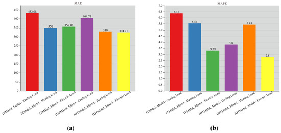
Figure 15.
Error-Stacking Diagram of ITMMoL Model and IDTMMoL Model. (a) MAE. (b) MAPE.
5.4.2. Analysis of the Effectiveness of the Model Optimization Strategy
In order to verify the effectiveness of our IDTMMoL model in the network layer structure TMMoL module, this paper sets up the control IDCLSTM model. The comparison model is a traditional multi-task load forecasting model based on parameter hard sharing. The traditional multi-task learning mechanism uses the LSTM layer as the sharing layer and then connects the fully-connected layer as the prediction output to achieve multi-load forecasting.
As shown in Figure 16, we show the performance comparison of the IDCLSTM model and the IDTMMoL model on the test set for a certain period of time for cooling, heating, and electric loads. It can be seen that in the prediction effect of the electric load, the proposed IDTMMoL model and the traditional multi-task IDCLSTM model can achieve a better prediction effect, and the prediction curve has a higher degree of fit to the real curve. The IDTMMoL model shows a better prediction effect than the IDCLSTM model. However, through the comparison of some details, the IDTMMoL model can still maintain a good fitting effect in the part where the curve fluctuates violently and the predicted value is closer to the real value, while the prediction error of the IDCLSTM model is improved, and the fit is not good.
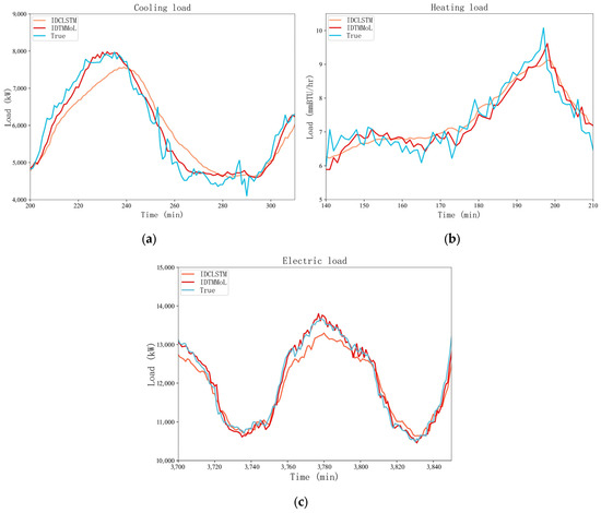
Figure 16.
Comparison of Prediction Effects. (a) Cooling load. (b) Heating load. (c) Electric load.
In addition, since the fluctuation of the cooling load and heating load is more severe than that of the electric load, the training of the model is more difficult and prone to over-fitting or under-fitting. It can be seen from Figure 16 that the IDCLSTM model is more conservative in the prediction of cooling and heating loads, and the fluctuation of the prediction curve is gentle in the face of large fluctuations in cooling and heating loads. As can be seen in Table 3, the MAPE percentage of the cooling load in the IDCLSTM model is 6.98%, while the IDTMMoL model still maintains a good predictive ability, and its MAPE index percentage is 3.8%, which is 3.18 percentage points lower than that of the IDCLSTM model. The reason for this is that using LSTM as the hard sharing layer cannot consider the correlation difference between multiple loads, resulting in providing the same weight value for the subtask layer, which affects the performance of the model. In contrast, the proposed IDTMMoL model achieves feature information sharing between multi-tasks by setting up multiple expert subnets. At the same time, the setting of the gating layer also avoids the interference of weak correlation information on subtasks. In addition, according to the fluctuation characteristics of subtasks and the correlation differences between multiple loads, the IDTMMoL model also sets different loss functions. Therefore, the IDTMMoL model achieves better prediction results.
The error comparison diagram of the two comparison models is presented by Figure 17. It can be seen here that our proposed IDTMMoL model performs better than the IDCLSTM model in the test set’s cooling, heating, and electric loads, and the MAPE error percentage and MAE error value are reduced. This also shows that the TCN layer in the IDTMMoL model can obtain the feature information of the long time series more than the CNN layer of the IDCLSTM model and mine the data. When the feature information is introduced into the LSTM layer, the LSTM unit layer in the IDTMMoL model can better refine these temporal and spatial features. Therefore, the prediction effect of our IDTMMoL model is better.
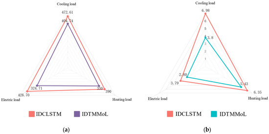
Figure 17.
Error-Stacking Diagram of IDCLSTM Model and IDTMMoL Model. (a) MAE error. (b) MAPE error.
6. Conclusions
In order to address the multi-load forecasting problem of integrated energy systems, this paper designs the data feature preprocessing link and model selection link and proposes a multi-load forecasting method for an integrated energy system based on the iForest algorithm and dynamic orbit method. Through the example analysis, the following conclusions are obtained.
- The Lonely Forest algorithm can deal with the outlier problem in high-dimensional big data and has the characteristics of high processing accuracy and fast calculation speed.
- The dynamic orbit method can effectively eliminate the hidden outliers in the time series, and the cleaning effect is good, which provides a good foundation for the neural network prediction model.
- The coupling relationship between load data in the integrated energy system is complex. The AR method can analyze the time series characteristics of the load, and the MIC method can mine the spatial characteristics between the loads and construct a high-dimensional feature matrix with strong correlation, which lays a foundation for improving the accuracy of the prediction model.
- Through the reasonable design of the TCN-MMoL network structure, the coupling characteristics of historical data are better learned from the three aspects of data feature capture, learning, and multi-task allocation, and the prediction accuracy is improved, which proves the effectiveness of the algorithm in the time series feature sequence.
The research results of this paper provide a new solution and method for the multi-load forecasting problem of integrated energy systems, which is of great significance to promote the intelligence and efficiency of an integrated energy system.
Based on the findings of this study, our future research direction can be extended to more application scenarios, such as wind power and photovoltaic power forecasting and electricity price forecasting for integrated energy systems.
Author Contributions
Methodology, S.W.; Supervision, H.M. and A.M.A. and B.W.; Visualization, L.X. and G.W. and S.Z. and L.Q.; Writing—original draft, S.W. All authors have read and agreed to the published version of the manuscript.
Funding
This research received no external funding.
Institutional Review Board Statement
Not applicable.
Informed Consent Statement
Not applicable.
Data Availability Statement
Not applicable.
Conflicts of Interest
The authors declare no conflict of interest.
References
- Luo, Z.; Liu, D.; Shen, X.; Wang, G.; Yu, P.; Li, Z. A review of research on operation optimization techniques for integrated energy systems. Electr. Power Constr. 2022, 43, 3–14. [Google Scholar]
- Xi, D.; Xiaoyan, Z.; Shenghan, W.; Chutong, W.; Houbao, X.; Chuangxin, G. Low-carbon planning of regional integrated energy system considering the optimal construction timing under the dual-carbon goal. High-Volt. Technol. 2022, 48, 2584–2596. [Google Scholar]
- Zhou, Q.; Sun, Y.; Lu, H.; Wang, K. Learning-based green workload placement for energy internet in smart cities. J. Mod. Power Syst. Clean Energy 2022, 10, 91–99. [Google Scholar] [CrossRef]
- Dong, Y.; Shan, X.; Yan, Y.; Leng, X.; Wang, Y. Architecture, key technologies and applications of load dispatching in China power grid. J. Mod. Power Syst. Clean Energy 2022, 10, 316–327. [Google Scholar] [CrossRef]
- Chen, L.; Xu, Q.; Yang, Y.; Gao, H.; Xiong, W. Community integrated energy system trading: A comprehensive review. J. Mod. Power Syst. Clean Energy 2022, 10, 1445–1458. [Google Scholar] [CrossRef]
- Pan, X.; Wenlong, F.; Qipeng, L.; Shihai, Z.; Renming, W.; Jiaxin, M. Stability analysis of hydro-turbine governing system with sloping ceiling tailrace tunnel and upstream surge tank considering nonlinear hydro-turbine characteristics. Renew. Energy 2023, 210, 556–574. [Google Scholar]
- Peng, L.; Fan, Z.; Xiyuan, M.; Senjing, Y.; Zhuolin, Z.; Ping, Y.; Zhuoli, Z.; Sing, L.C.; Lei, L.L. Multi-Time Scale Economic Optimization Dispatch of the Park Integrated Energy System. Front. Energy Res. 2021, 9, 743619. [Google Scholar]
- Guo, X.; Lou, S.; Wu, Y.; Wang, Y. Low-carbon operation of combined heat and power integrated plants based on solar-assisted carbon capture. J. Mod. Power Syst. Clean Energy 2021, 10, 1138–1151. [Google Scholar] [CrossRef]
- Sobhan, D.; Masoud, R.; Farshad, F.A.S.; Amir, A.; Reza, S.M. An integrated model for citizen energy communities and renewable energy communities based on clean energy package: A two-stage risk-based approach. Energy 2023, 277, 127727. [Google Scholar]
- Zhu, J.; Liu, H.; Ye, H. Summary of research on optimal operation of integrated energy system in the park. High Volt. Technol. 2022, 48, 2469–2482. [Google Scholar]
- Yan, C.; Bie, Z.; Liu, S.; Urgun, D.; Singh, C.; Xie, L. A reliability model for integrated energy system considering multi-energy correlation. J. Mod. Power Syst. Clean Energy 2021, 9, 811–825. [Google Scholar] [CrossRef]
- Zhang, Y.; Xie, X.; Chen, X.; Hu, S.; Zhang, L.; Xia, Y. An Optimal Combining Attack Strategy Against Economic Dispatch of Integrated Energy System. IEEE Trans. Circuits Syst. II Express Briefs 2023, 70, 246–250. [Google Scholar] [CrossRef]
- Jizhong, Z.; Hanjiang, D.; Shenglin, L.; Ziyu, C.; Tengyan, L. Review of data-driven load forecasting for integrated energy systems. Chin. J. Electr. Eng. 2021, 41, 7905–7924. [Google Scholar]
- Chandrahas, M.L.D.G. Deep Machine Learning and Neural Networks: An Overview. IAES Int. J. Artif. Intell. 2017, 6, 66–73. [Google Scholar]
- Schmidhuber, J. Deep learning in neural networks: An overview. Neural Netw. 2015, 61, 85–117. [Google Scholar] [CrossRef] [PubMed]
- Ping, F.; Wenlong, F.; Kai, W.; Dongzhen, X.; Kai, Z. A compositive architecture coupling outlier correction, EWT, nonlinear Volterra multi-model fusion with multi-objective optimization for short-term wind speed forecasting. Appl. Energy 2022, 307, 118191. [Google Scholar]
- Shi, J.; Tan, T.; Guo, J. Multivariate load forecasting of park-type integrated energy system based on deep structure multi-task learning. Grid Technol. 2018, 42, 698–707. [Google Scholar]
- Wang, S.; Wang, S.; Chen, H.; Gu, Q. Multi-energy load forecasting for regional integrated energy systems considering temporal dynamic and coupling characteristics. Energy 2020, 195, 116964. [Google Scholar] [CrossRef]
- Yang, N.; Yang, C.; Wu, L.; Shen, X.; Jia, J.; Li, Z.; Chen, D.; Zhu, B.; Liu, S. Intelligent Data-Driven Decision-Making Method for Dynamic Multisequence: An E-Seq2Seq-Based SCUC Expert System. IEEE Trans. Ind. Inform. 2021, 18, 3126–3137. [Google Scholar] [CrossRef]
- Tan, Z.; De, G.; Li, M.; Lin, H.; Yang, S.; Huang, L. Combined electricity-heat-cooling-gas load forecasting model for integrated energy system based on multi-task learning and least square support vector machine. J. Clean. Prod. 2020, 248, 119252. [Google Scholar] [CrossRef]
- Zhou, D.; Ma, S.; Hao, J.; Han, D.; Huang, D.; Yan, S.; Li, T. An electricity load forecasting model for Integrated Energy System based on BiGAN and transfer learning. Energy Rep. 2020, 6, 3446–3461. [Google Scholar] [CrossRef]
- Long, C.; Zhongyang, H.; Jun, Z.; Wei, W. Review of data-driven integrated energy system operation optimization methods. Control Decis.-Mak. 2021, 36, 283–294. [Google Scholar]
- Nan, Y.; Tao, Q.; Lei, W.; Yu, H.; Yuehua, H.; Chao, X.; Lei, Z.; Binxin, Z. A multi-agent game based joint planning approach for electricity-gas integrated energy systems considering wind power uncertainty. Electr. Power Syst. Res. 2021, 204, 107673. [Google Scholar]
- Zihan, M.; Shouxiang, W.; Qianyu, Z.; Zhijie, Z.; Liang, F. Reliability evaluation of electricity-gas-heat multi-energy consumption based on user experience. Int. J. Electr. Power Energy Syst. 2021, 130, 106926. [Google Scholar]
- Smiti, A. A critical overview of outlier detection methods. Comput. Sci. Rev. 2020, 38, 100306. [Google Scholar] [CrossRef]
- Xu, S.; Li, Y.; Yuan, Q. A combined pruning method based on reinforcement learning and 3σ criterion. J. Zhejiang Univ. (Eng. Ed.) 2023, 57, 486–494. [Google Scholar]
- Kai, M.; Rencai, Z.; Jie, Y.; Debao, S. Collaborative optimization strategy of integrated energy system considering demand response. Renew. Energy 2023, 41, 676–684. [Google Scholar]
- Yulong, Y.; Xinge, W.; Ziye, Z.; Rong, J.; Chong, Z.; Songyuan, L.; Pengyu, Y. Integrated energy optimization scheduling considering extended carbon emission flow and carbon trading bargaining model. Power Syst. Autom. 2023, 47, 34–46. [Google Scholar]
- Caicedo, J.E.; Agudelo Martínez, D.; Rivas Trujillo, E.; Meyer, J. A systematic review of real-time detection and classification of power quality disturbances. Prot. Control Mod. Power Syst. 2023, 8, 3. [Google Scholar] [CrossRef]
- Xinyu, W.; Ke, L. LF Ant Colony Clustering Algorithm with Global Memory. J. Comput. Eng. Appl. 2019, 55, 52–57+113. [Google Scholar]
- Xiong, K.; Ding, Q.; Zhu, H. Fault detection of chillers based on isolated forest and KDE-LOF. Comput. Appl. Softw. 2023, 40, 84–89. [Google Scholar]
- Shaolan, L.; Huawei, W.; Zhaoguo, H.; Lingzi, C. Unmanned Aerial Vehicle Anomaly Detection Algorithm Based on Ensemble Isolation Forest. Radio Eng. 2022, 52, 1375–1385. [Google Scholar]
- Feilu, H.; Wei, G.; Hexiong, C.; Zhenhong, Z.; Dongyang, Y. Traffic anomaly detection based on iForest and LOF. Comput. Appl. Res. 2022, 39, 3119–3123. [Google Scholar]
- Lesouple, J.; Baudoin, C.; Spigai, M. Generalized isolation forest for anomaly detection. Pattern Recognit. Lett. 2021, 149, 109–119. [Google Scholar] [CrossRef]
- Mikhail, T.; Paweł, K. A probabilistic generalization of isolation forest. Inf. Sci. 2022, 584, 433–449. [Google Scholar]
- Huichun, X.; Yuan, N.; Jiangong, Z.; Yanzhao, W.; Yemao, Z.; Zheyuan, G. Discrimination of measured outliers of ground synthetic electric field of DC transmission lines based on ARIMA and exponential smoothing method. High Volt. Technol. 2023, 49, 2161–2170. [Google Scholar]
- Su, Y.; Cui, C.; Qu, H. Time series prediction based on self-attention moving average. J. Nanjing Univ. (Nat. Sci.) 2022, 58, 649–657. [Google Scholar]
- Reza, M.M.; Salman, B. Modeling the stochastic mechanism of sensor using a hybrid method based on seasonal autoregressive integrated moving average time series and generalized estimating equations. ISA Trans. 2021, 125, 300–305. [Google Scholar]
- Surria, N.; Muhammad, A.U.N.; Muhammad, M.; Ahmed, A. Hybrid exponentially weighted moving average control chart using Bayesian approach. Commun. Stat.-Theory Methods 2022, 51, 3960–3984. [Google Scholar]
- Pengfei, Z.; Bo, H.; Jinsong, H.; Zhanshuo, H.; Hengyu, L.; Yubo, L. Short-term spatial load forecasting method based on spatio-temporal graph convolutional network. Power Syst. Autom. 2023, 47, 78–85. [Google Scholar]
- Xiaojian, W.; Yihua, W.; Aichun, W.; Yao, L.; Ruixue, Z. LSTM-GRU vehicle trajectory prediction based on Dropout and attention mechanism. J. Hunan Univ. (Nat. Sci. Ed.) 2023, 50, 65–75. [Google Scholar]
- Zhonglin, L.; Jie, G.; Lu, M. Short-term load forecasting of integrated energy system based on coupling characteristics and multi-task learning. Power Syst. Autom. 2022, 46, 58–66. [Google Scholar]
- Xurui, H.; Fengyuan, Y.; Bo, Y.; Jun, P.; Qin, X. Electric-thermal short-term load forecasting method of park integrated energy system based on Transformer network and multi-task learning. China South. Power Grid Technol. 2023, 17, 152–160. [Google Scholar]
- Haixiang, Z.; Ruiqi, X.; Jingxuan, L.; Yuwei, C.; Zhinong, W.; Guoqiang, S. Multi-Task Short-Term Load Forecasting for Users Based on Multi-Dimensional Fusion Features and Convolutional Neural Network. Autom. Electr. Power Syst. 2023, 47, 69–77. [Google Scholar]
- Wang, B.; Bai, Y.; Xing, H. A joint prediction method for ultra-short-term power of regional multi-photovoltaic power stations based on STL and MMoE multi-task learning. J. Power Syst. Autom. 2022, 34, 17–23+31. [Google Scholar]
- Li, C.; Li, G.; Wang, K. A multi-energy load forecasting method based on parallel architecture CNN-GRU and transfer learning for data deficient integrated energy systems. Energy 2022, 259, 124967. [Google Scholar] [CrossRef]
- Li, Y.; Bu, F.; Gao, J.; Li, G. Considering the low-carbon optimal operation of the integrated energy system of solar thermal power station and LAES. Electr. Meas. Instrum. 2022, 378, 134540. [Google Scholar]
- Wu, C.; Yao, J.; Xue, G. Load forecasting of integrated energy system based on MMoE multi-task learning and long short-term memory network. Power Autom. Equip. 2022, 42, 33–39. [Google Scholar]
- Qian, K.; Lv, T.; Yuan, Y. Integrated energy system planning optimization method and case analysis based on multiple factors and a three-level process. Sustainability 2021, 13, 7425. [Google Scholar] [CrossRef]
- Rui, H.; Lingli, Z.; Feng, G. Short-term Power Load Forecasting Method Based on Variational Modal Decomposition for Convolutional Long-short-term Memory Network. Mod. Electr. Power 2023. [Google Scholar] [CrossRef]
- Jiang, C.; Ai, X. A review of collaborative planning methods for integrated energy systems in industrial parks. Glob. Energy Internet 2019, 2, 255–265. [Google Scholar]
- Liu, Y.; Huang, Y.; Tan, H. Online prediction method of wing flexible baseline based on autoregressive model. J. Beijing Univ. Aeronaut. Astronaut. 2022, 48. [Google Scholar] [CrossRef]
- Cen, L.; Li, J.; Lin, C.; Wang, X. Approximate query processing method based on deep autoregressive model. Comput. Appl. 2023, 43, 2034. [Google Scholar]
- Shuliang, W.; Surapunt, T. Bayesian Maximal Information Coefficient (BMIC) to reason novel trends in large datasets. Appl. Intell. 2022, 52, 10202–10219. [Google Scholar] [CrossRef]
- Ling, Q.; Zhang, Q.; Zhang, J. Prediction of landslide displacement using multi-kernel extreme learning machine and maximum information coefficient based on variational mode decomposition: A case study in Shaanxi, China. Nat. Hazards 2021, 108, 925–946. [Google Scholar] [CrossRef]
- Lawrence Berkeley National Laboratory. EnergyPlus-Engineering Documentation: The Reference to EnergyPlus Calculations; University of Illinois: Chicago, IL, USA; Ernest Orlando Lawrence Berkeley National Laboratory: Berkeley, CA, USA, 2001.
- Yue, W.; Liu, Q. Multivariate load forecasting of integrated energy system based on PCC-LSTM-MTL. J. Shanghai Electr. Power Univ. 2022, 38, 483–487+494. [Google Scholar]
- Wang, Y.; Liu, E.; Huang, Y. Data-driven short-term multi-load forecasting of integrated energy systems. Comput. Eng. Des. 2022, 43, 1435–1442. [Google Scholar]
Disclaimer/Publisher’s Note: The statements, opinions and data contained in all publications are solely those of the individual author(s) and contributor(s) and not of MDPI and/or the editor(s). MDPI and/or the editor(s) disclaim responsibility for any injury to people or property resulting from any ideas, methods, instructions or products referred to in the content. |
© 2023 by the authors. Licensee MDPI, Basel, Switzerland. This article is an open access article distributed under the terms and conditions of the Creative Commons Attribution (CC BY) license (https://creativecommons.org/licenses/by/4.0/).