Article

Underground Logistics Network Design for Large-Scale Municipal Solid Waste Collection: A Case Study of Nanjing, China

1
Faculty of Architecture, Civil and Transportation Engineering, Beijing University of Technology, Beijing 100124, China
2
Institute of Defense Engineering, Academy of Military Sciences PLA, Beijing 100850, China
3
School of Science, Nanjing University of Science and Technology, Nanjing 210094, China
4
School of Defense Engineering, Army Engineering University of PLA, Nanjing 210007, China
5
The First Geological Brigade, Jiangsu Provincial Bureau of Geology and Mineral Resources, Nanjing 210041, China
*
Authors to whom correspondence should be addressed.
Sustainability 2023, 15(23), 16392; https://doi.org/10.3390/su152316392
Submission received: 10 October 2023 / Revised: 15 November 2023 / Accepted: 24 November 2023 / Published: 28 November 2023
(This article belongs to the Special Issue Sustainable Waste Management and Utilization)

Abstract

:
The challenges arising from the management of municipal solid waste (MSW) have a profound impact on the sustainable development of urban areas. As a sustainable solution, the transportation of MSW underground offers the potential to alleviate traffic congestion and reduce environmental pollution. In this study, we propose the implementation of a large-scale underground waste collection system (UWCS). To begin, a comprehensive operational process for the UWCS is designed based on an intelligent technology system, including facility operation, processing workflow, and technical parameters. Additionally, network planning methods for the UWCS are presented. A mixed-integer linear programming model is formulated with the objective of minimizing total cost. This model determines the optimal location and allocation of nodes within the network, as well as the pipeline layout and flow direction. Given the computational complexity, a hybrid optimization method, namely the genetic greedy algorithms and genetic variable neighborhood search algorithms (GGA-GVNS), is devised to obtain high-quality solutions for the model. Finally, to validate the efficacy of the proposed method, a simulation is conducted in the central city of Nanjing, China. The results demonstrate that the implementation of the UWCS network in Nanjing’s city center can yield an annual benefit of USD 5.99 million. Moreover, a sensitivity analysis reveals further MSW management-related insights and long-term planning strategies.

1. Introduction

With the rapid growth of the urban population, the production of municipal solid waste (MSW) has witnessed a significant increase, accompanied by a diversification in the types of waste [1,2,3]. The clearance and processing volume of MSW in China experienced a notable rise from 191.419 million tons in 2015 to 2420.62 million tons in 2019, reflecting a year-on-year growth rate of 20.9%. It is expected to reach 409 million tons by 2030. Effectively managing MSW has become a pressing issue for cities. In traditional methods of MSW processing, the problem of accumulation arises due to limited waste treatment capacity, leading to long-term environmental and human health concerns [4,5]. Waste classification offers several advantages, such as improving the utilization rate of waste resources, effectively protecting the ecological environment, and facilitating sustainable urban development [6]. Notably, in recent years, many developing countries, including China, have started implementing waste classification initiatives [7,8]. However, the implementation of waste classification has also encountered certain challenges. Residents’ awareness of waste classification has caused improper source sorting, necessitating the use of different types of vehicles for waste transportation—a factor that further escalates transportation costs, urban traffic congestion, and greenhouse gas emissions [9,10,11]. Therefore, with the advent of technologies like intelligent classification and smart garbage collection systems, the concept of MSW intelligent classification has gained considerable attention within society. Based on this technology, the undergrounding of MSW has also started to experiment in many cities and countries. For instance, in Tongzhou, Beijing, China, a pneumatic waste collection system primarily transported kitchen waste and other waste through underground transport pipes. The classified waste was pre-treated in the pipes and then moved to the transport truck inside the container. As early as 1975 in New York, pneumatic underground pipes realized waste collection from 16 high-rise buildings in Manhattan to the transfer station in Queens [12], among other things.
Therefore, we propose a groundbreaking and all-encompassing subterranean waste collection system, referred to as the underground waste collection system (UWCS). Firstly, the distinctiveness of the UWCS lies in its meticulous process design. Following the automated classification of MSW, diverse types of waste necessitate dedicated pipelines for transportation. However, the criteria for classifying MSW vary across different countries [7]. During transportation, it is essential to align the flow direction and size of the pipelines with the movement of waste between facilities, all coordinated with the speed of the vehicles [13]. At the same time, facility capacity, equipment treatment capacity, and treatment plant size need to be reasonably designed according to the amount of waste generated to ensure efficient transportation [14]. Furthermore, effective information management is indispensable between the automated classification equipment, the intelligent waste control system, and the smart city digital platform, facilitating the digitalization and refinement of MSW underground transportation [15,16,17]. Secondly, the UWCS can also be defined as an extensive and intricate reverse logistics network transportation system. The UWCS integrates a series of MSW logistics activities, including automatic classification, collection, pretreatment, transfer, and ultimate disposal, into a set of pipeline infrastructure networks with sufficient capacity. The location of underground network facilities is intricately based on the existing transportation system, with certain facilities either clustered together or directly relocated beneath the surface. In addition to common goals such as minimizing operating costs and minimizing transport distances as in traditional MSW transportation system network design, the overall design of the UWCS network is influenced by characteristics such as the high cost and irreversibility of underground works [14].
In summary of existing studies, we find that scholarly investigations into the subterranean collection of MSW have been scarce, primarily focused on evaluating the feasibility and benefits of underground automatic vacuum collection systems [18,19,20]. With the advancing strides in intelligent technology and the initial implementation observed in select new cities, UWCS represents an emerging solution to cope with the ever-growing MSW production. Next, most researchers have concentrated on the study of small-scale MSW collecting systems within cities. Instead, there is very little research on the design and network planning of large-scale underground MSW collection systems. Furthermore, network planning can be made more efficient and decision-making easier through the use of mixed-integer planning models to quantify the network layout of large-scale urban domestic garbage collection systems. To fill the gap, this study proposes a network design method for a large-scale automated waste collection system as a case study in the central city of Nanjing, China. Firstly, we provide an overview of the various technical techniques and create the entire suite of UWCS operational processes. Secondly, a mixed-integer linear programming (MILP) model and solution algorithm are introduced to obtain the location of node facilities and the waste distribution between the facilities. Furthermore, a sensitivity analysis is conducted to examine the model’s viability across various parameters. By providing an efficient underground waste collection system for Nanjing, this study’s findings will facilitate rational decision-making by local authorities concerning the management of MSW.
The contributions of this study mainly lie in two aspects: (1) the operation process of UWCS and the idea of facility siting layout are designed based on the intelligent technology system. This system generates fresh concepts for both the UWCS network layout and the network planning of other subterranean transportation systems; (2) from the standpoint of the application, the research findings broaden the scope of the MSW collecting and reverse logistics research domains and enhance the functional design of MSW transportation systems. In addition, this study offers new ideas and quantitative optimization approaches for linear or network-based complex engineering projects. The supplied case study provides additional insights for research and practice.
The novelties of this study are two. Firstly, we designed an automatic intelligent transportation system encompassing the entire process from UCP-CCP-UTS-treatment plants. The operational flow of the system was designed and described in detail, providing an original planning design for the automatic, reliable, and environmentally friendly implementation of waste reverse logistics at the urban level. Secondly, considering the matching with existing facilities and network operations, the optimal layout of underground facilities, pipelines, and the waste flow direction was determined through the utilization of a mixed-integer linear programming model, which was then validated and efficiently solved by a GGA-GVNS hybrid optimization algorithm. The proposed method for optimizing network layout brings a new perspective to the planning of the UWCS network.
The remainder of this paper is organized as follows: Section 2 offers an extensive review based on the body of current research. Section 3 describes the system operating process, technological specifications, and optimization issues of UWCS. In Section 4, the mathematical model is presented. The model’s solution algorithm is created in Section 5. The simulation results of Nanjing UWCS network schemes are discussed in Section 6. Finally, Section 7 summarizes the findings and points out future research directions.

2. Literature Review

2.1. MSW Underground Collection System

MSW collection and transportation are important parts of MSW management. At present, the MSW transportation system is composed of three types of facilities: collection points, transfer stations, and treatment plants. The traditional MSW transportation starts at the collection points, followed by transfer and pretreatment at transfer stations, and finally the final disposal at treatment plants [21,22,23]. With the development of intelligent technology, the process of waste collection has started to consider intelligent waste classification, and different types of vehicles are used to transport the classified waste, which improves the efficiency of waste disposal but also increases the cost of MSW management [24,25,26].
The use of underground spaces for collecting waste began in the 1960s, and more than 1600 automated vacuum collection system solutions are under construction or in operation in more than 30 countries in Europe, North America, and Australia [27]. In Shanghai, a network of container railroad tunnels was planned deep underground in the city for the automatic transport of MSW between municipal waste collection points and waste incineration plants [28]. Nakou et al. studied the construction costs of a vacuum underground waste collection network that covered several neighborhoods in Athens [20]. In Singapore, pneumatic waste collection systems have been implemented in some new buildings and private housing estates, where an underground pipe network conveys waste to collection points via the power of vacuum suction [7].
Unlike the most recent studies, the UWCS suggested in this study expands the planning horizon from a small urban region to an urban supply chain. Additionally, it incorporates intelligent transportation and automatic trash sorting technologies into the design of the system’s network structure and operating process. Furthermore, the proposed hybrid optimization technique employs basic but efficient algorithms and a decomposition strategy, which could be a much more generalized alternative for UWCS planning in megacities.

2.2. MSW Collection System Network Planning

In the design of reverse logistics networks, many scholars have focused on system design, network models, and algorithms. In terms of network modeling, Tsydenova et al. proposed the optimized design of the concrete network and established a bi-objective mixed-linear optimization model with a minimum cost of recycling the network [29]. This model defines the material flow in an integrated regional recycling network. Oyola-Cervantes and Amaya-Mier designed a reverse logistic system applicable to large complete tires discarded in decentralized mining sites [30]. A MILP model was developed to determine the optimal network of scrap road tires, including decisions on facility siting and transportation amounts, so as to maximize the profitability of the reverse logistics network. Trochu et al. proposed a random planning model of a two-stage reverse logistics network design with uncertainty and dynamic supply source locations [31]. The main objective of the optimization model was to maximize the expected profit generated by the sale of recycled materials to the secondary market. Govindan et al. proposed a multi-item, multi-period, and bi-objective model to design a green reverse network for medical waste and obtained the best location of the facility and vehicle routes with the optimization objective of minimizing total cost and population risk [32]. Yoosefloo et al. have designed a network for sustainable MSW management under uncertainty, seeking sustainability from two qualitative and quantitative aspects [33].
In terms of solution algorithm, Blazquez and Paredes-Belmar proposed a two-stage MILP model based on a two-stage MSW collection system and used the large neighborhood search algorithm in the second stage to find good feasible vehicle path solutions [34]. Lu et al. proposed an intelligent waste classification and collection system and optimized the problem of waste collection by establishing a bi-objective mathematical planning model. A new multi-objective hybrid algorithm based on whale optimization and genetic algorithms has determined the problem of vehicle route planning in different echelons and the problem of trash bin allocation [35]. Shang et al. introduced a distributionally robust cluster-based hierarchical hub location problem for the integration of urban and rural public transport systems at the strategic level, and a variable neighborhood search algorithm and a population-and-searching-based heuristic algorithm were designed to handle the realistic-sized instances [36]. Hashemi-Amiri et al. applied the chance-constrained programming approach to deal with the profit uncertainty gained from waste recycling and recovery activities. Furthermore, some of the most proficient multi-objective meta-heuristic algorithms are applied to address the complexity of the problem [37].
Traditional above-ground MSW collection system research has yielded broad knowledge in terms of network design and models. However, the underground waste collection plan is different. Firstly, the deployment of waste pipelines is one-time and irreversible. Waste transport in the underground network must meet the layout of the fixed infrastructure and the established network topology. Secondly, considering the different loads of nodes and pipelines, a multi-level network topology is required to schedule underground freight transportation. Finally, effective information control among the automatic classification equipment, intelligent waste control system, and digital platform of UWCS requires the integrated planning of transportation paths, nodes, and pipeline locations of the UWCS network. Therefore, by building a mixed-integer linear programming model and creating a hybrid optimization method based on the features of underground waste collection, this study is able to determine the facility layout and capacity allocation of the UWCS network.

3. Prototyping UWCS Network

The considered UWCS network includes the underground node facilities, network topology, operational flow of facilities and equipment, and related technical systems. This section describes the system prototyping and the assumptions and modeling boundaries of the UWCS network design problem.

3.1. UWCS Physical Components

3.1.1. Node Facilities

Considering the capacity of the facility and the environmental impact of the waste itself, in the UWCS, waste cannot be excessively detained after reaching the corresponding underground node. Instead, they should be transferred directly to the next node for processing. By setting one or two transit layers between the waste generation point and the processing plant, it can greatly improve transportation efficiency and system service capabilities. Based on the above planning principles, the node facilities are divided into the following four layers:
(1)
Underground collection point (UCP)
The UCP plays a role in docking the surface with underground networks. Residents directly put MSW into the UCPs, which are then automatically classified, initially separated, compacted, boxed, and stacked at the loading and unloading platform. In this paper, the centers of the residential community are used as UCPs.
(2)
Concentrated collection point (CCP)
The CCP is one of the optimization targets, with waste pre-treatment or a temporary storage function connecting the upper UCPs and the lower underground transfer stations. The number and distribution of CCPs directly affect system services. In this paper, the candidate set of CCPs is first determined by an E-Topsis evaluation model, and then the optimal location of CCPs is determined by a mixed-integer linear programming model with a heuristic algorithm.
(3)
Underground transfer station (UTS)
The UTS is also one of the optimization goals, with a waste transfer function connecting the upper CCPs and the lower treatment plant. The waste transfer capacity of UTSs is the main barrier to system service performance. In this paper, the optimal position of UTSs is determined in the same way as CCPs.
(4)
Processing plants
Because MSW can be divided into four types of waste, there are also four types of processing plants: recyclable processing plant (RPP), comprehensive kitchen waste disposal center (CKWDC), hazardous waste collection center (HWCC), and incineration plant (IP), with final disposal functions. In this article, the location of the treatment plant has been determined outside the city.

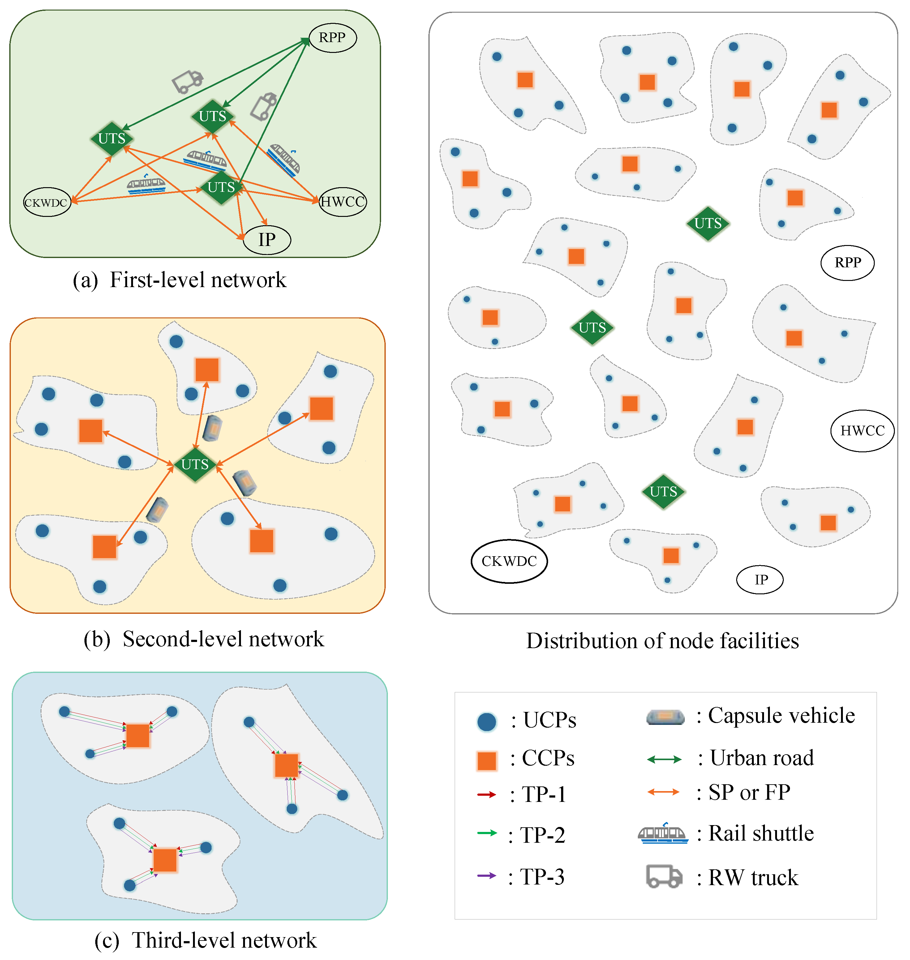
3.1.2. Network Topology

As depicted in Figure 1, the UWCS network designed in this paper has three levels.
The topology characteristics of the third-level network can be described as a hub-and-spoke structure, and the transportation path is from UCPs to CCPs. Given the different types of MSW and packing methods, the third-level pipeline (TPs) is set up in a three-lane unidirectional form to ensure that each type of waste enters the corresponding pipeline for transportation. The specifications of pipelines TPs-1, TPs-2, and TPs-3 are the same. The transportation process in the network is roughly described as follows: First of all, the residents manually bring MSW to UCPs and put them into the port of intelligent waste devices. The intelligent waste classification devices automatically divide the waste into four categories: kitchen waste (KW), other waste (OW), recyclable waste (RW), and hazardous waste (HW), which then enter the mobile storage waste unit. The device contains a temporary storage section that works together with the central control system to control the operation of the system. Among them, TP-1 transports KW, TP-2 transports OW, and TP-3 transports RW and HW. In the TP-3 pipeline, RW directly enters the pneumatic pipe, while HW temporarily exists in Container 4, and then enters the pipeline when it reaches a certain amount.
The topology characteristics of the secondary network can also be described as a hub-and-spoke structure, and the transportation path is from CCPs to UTSs. The second-level pipelines (SPs) of the network are set up with a single lane and use automated guided vehicles for staggered transportation. The transportation process is described as follows: MSW transported from TP-1, TP-2, and TP-3 enters the loading and unloading platforms of CCPs. At this time, the four types of waste are transported to different disposal points. KW is transported from the loading and unloading platform to the pre-processing device of the kitchen waste, where KW is squeezed, hydraulic, and then loaded into Container 1. OW is transported to other garbage-compressed devices, and it is compressed and loaded into Container 2. RW is transported to the recyclable waste classification device, further classified, and then loaded into Container 3. HW does not process it directly into the loading and unloading platform. When the sensor in the container detects that the waste is full, the control system will call the robotic arm to transport the container to the vehicle, which will then be transported along the SPs. The quality specifications of the container should be determined in advance to avoid violations of the carrier capacity of vehicles and pipelines.
The topological characteristics of the first-level network can be described as a star structure. Each UTS has multiple allocation processing plants. In order to reduce the complexity of the model, there is no connection between any two UTSs. In this network, use the first-level pipelines (FPs) and cooperate with automated guided vehicle staggered transport. The transportation process is as follows: MSW transported from the SPs enters the loading platform at UTSs, where various types of containers are unloaded from the vehicles. When the system detects that the container meets the transport quantity, the robotic arm is called to put the container on the transport vehicle, and then the vehicle is transported along the FPs to different processing plants, respectively. In particular, because of the small variation in RW generation and the relatively fixed frequency of dispatch, this paper designs RW to be transported to RPP using trucks. Of course, according to the actual local needs, underground pipelines can also be used for transportation, and they have no influence on the system network analysis and model study.
The entire network’s operations are adaptively controlled. The MSW conveying process is completed in a fully enclosed state from start to finish, without any manual operation or direct contact with waste.

3.2. UWCS Technology Components

The treatment of MSW in the underground is similar to that of traditional MSW but still requires some necessary equipment and technology. Specifically, KW’s pre-processing unit, OW’s compression unit, and KW’s classification unit. In particular, the unique technologies required for UWCS mainly include two categories, namely MSW intelligent classification technologies and transportation technologies. In terms of MSW intelligent classification, a smart trash bin prototype designed by Clean Robotics in the United States and a smart waste container developed by the French UZE company both automatically discriminate and classify the types of waste [38,39]. In terms of MSW underground transportation technology, it mainly includes underground pipelines, transportation vehicles, and control systems. Underground pipelines are directly in contact with MSW transported by high-speed transportation. MSW has a certain shape and size and contains different components, which may have adverse effects on pipelines, so it is particularly important to the choice of pipelines [1]. The type of pipeline mainly includes pneumatic pipelines, vacuum pipes, and electric pipelines. Fernández et al. proposed a control system equipped with an automatic vacuum waste collection system (AVWC), which can be used to determine the time interval for clearing the entrance [27]. This control technology is particularly important for the AVWC system to reduce energy consumption. Among them, the UWCS can refer to the technical parameters as shown in Table 1.
According to the facility capacity, transport vehicle load, and waste type, the main transportation technology systems used in this paper are selected from Table 1. For the TPs, due to the shorter transportation distance of the third-level network, it can be transported at any time. It is easy to use pneumatic pipelines. For FPs and SPs, the PCP or UCT vehicle mode can better meet transportation needs. It can also be selected according to local needs.
Related underground transportation and pipeline technology have been widely used in municipal and transportation fields such as subways, underground highways, and public transport tunnels, which also provides a solid foundation for UWCS transportation technology.

3.3. Modeling Boundary and Hypotheses

The UWCS network we put forward in this study has a multi-level node topology structure. For the description of the network design problem of the system, it can be divided into two parts: (i) Determine the candidate position of CCPs and UTSs through E-Topsis; (ii) The decision-making of the problem mainly includes (a) determining the number and location of CCPs and UTSs; (b) determining the allocation of UCPs to CCPs or CCPs to UTSs; (c) determining the allocation of UTSs to various types of the processing plant. This problem is a classical three-tier capacity facility location–allocation problem (CFLAP), which is solved by an MILP model with the lowest system cost.
In order to keep the planning of the network consistent with reality, the following assumptions need to be added to adjust the boundaries of the problem. However, the problem can also be modified according to actual needs.
(i)
The amount and location of the waste at each demand point are known, and it remains stable and will not increase or decrease at different times within one year.
(ii)
The location of the processing plant is known, the processing capacity meets the needs, and the transportation capacity of FPs is not limited.
(iii)
In order to improve transportation efficiency, any two CCPs are not connected to each other, and any two UTSs are not connected to each other. The capacity of each CCP and each UTS is the same.
(iv)
The maintenance and installation costs of the pipeline and vehicle purchase costs are calculated into the fixed cost of the pipeline. The transportation cost of pneumatic pipelines is calculated into their fixed cost.
(v)
The driving distance between the nodes is straight, and it remains unchanged.
(vi)
Assuming that KW pre-processing, RW, OW, and HW collect transportation, it will not damage their quality.

4. Model Development

4.1. E-Topsis for Evaluating the Importance of Demand Points

When selecting CCPs and UTSs, node locations, capacity constraints, and distances to demand points and treatment plants need to be considered. This requires the importance of demand points as a priority assessment object when choosing (here, we define the importance of demand points as convenience from demand points to processing factories). The information entropy calculated in the indicator matrix is used to weigh the characteristics of the demand nodes, avoiding the influence of human subjective factors [40]. The technique for order preference by similarity to an ideal solution (TOPSIS) method is used to find the candidate nodes of the evaluation object in the target decision-making, which solves the problem of high requirements for samples. The TOPSIS method is a multi-subject and multi-attribute decision-making method, but the traditional TOPSIS method is mostly determined in terms of indicator weight and is more affected by human factors [40]. Therefore, we use improved entropy-weighted TOPSIS (E-Topsis) to comprehensively evaluate and rank the importance of demand points [41].
This paper uses three indicators of demand quantity (QD), regional accessibility (RA), and transportation cost (TC) to evaluate the importance of demand points in the system. Among them, the indicators QD and RA were obtained from Eftihia Nathanaila [42,43]. They believe that alleviating urban transportation and developing comprehensive transportation are two of the most significant features of sustainable cities. The indicator TC was obtained from Sagnak et al. [44,45]. They believe that transportation costs are the most important factor affecting the location of sustainable waste collection centers.
(1)
Demand quantity (DQ). Because the amount of MSW at each demand point will affect the flow of garbage transportation, the candidate locations of nodes at each level should be those with the highest possible generation:
I N 1 D Q = q i
where qi is the quantity of MSW generated per day at the demand point i.
(2)
Regional accessibility (RA). RA is defined as the convenience of MSW transportation from demand point i to processing plant n [46]. Regionally accessible indicator available time-distance function representation:
I N 2 R A = i I n N t i n S λ i n
where tin is the average transport time from the demand point i to the processing plant n, S is the transport distance within the region, and λ i n ∈(0, 1) is a time-sensitive factor.
(3)
Transportation cost (TC). TC is an important factor affecting the total cost of UWCS network construction. Therefore, the transportation path should be optimized to the maximum extent in the network design to minimize its transportation cost.
I N 3 T C = Q i n d i n L 1 + L 2 + L 3
where Qin is the amount of waste transported from demand point i to the processing plant n for each type of waste, din is the transportation distance from demand point i to the processing plant n, L1, L2, and L3 are the unit transportation costs (determined according to the local level).
The specific steps of the E-Topsis method of demand point importance evaluation are shown in Appendix A. Finally, the evaluation results are ranked. Select the first 8 demand points as the candidate points of UTSs, and select the 27 requirements of the secondary requirements as the candidate points of the CCPs.

4.2. MILP Model

4.2.1. Symbol Definition

The following notations in Table 2 are utilized for mathematical formulation.

4.2.2. Derivation of Objective Functions

The objective function F of the MILP model is to minimize the total cost of the UWCS, which mainly includes three parts. The first part of Equation (4) is the construction cost of CCPs, UTSs, TPs, SPs, and FPs. The second part is the procurement cost of CCP equipment. The third part is the total transportation cost, which combines (i) the transport cost of the SPs and the FPs, (ii) the road transport cost, and (iii) the disposal cost at CCPs.
Minimize   F = F 1 + F 2 + F 3
where
F 1 = 1 π j J h 2 x j + m M h 3 y m + C 3 i I j J d i j Z i j + C 2 j J m M d j m S j m + C 1 m M n N u U d m n W m n u F 2 = 1 π j J l η j F 3 = L 2 j J m M u U P j m u d j m + L 1 m M n 1 u a R m n u d m n + L 1 m M n 2 u b R m n u d m n             + L 1 m M n 4 u d R m n u d m n + L 3 m M n 3 u c R m n u d m n + v i I j J u U Q i j u

4.2.3. Derivation of Constraints

i I u U Q i j u η j c a p , j J
Q i j u c a p 3 1 , i I , j J , u a Q i j u c a p 3 2 , i I , j J , u b Q i j u c a p 3 3 , i I , j J , u c , d
d i j Z i j r 1 , i I , j J d j m S j m r 2 , j J , m M
j J u U P j m u c a p m , m M
u U P j m u c a p 2 , j J , m M
i I Q i j u = m M P j m u , j J , u a i I Q ij u = m M P j m u , j J , u b i I Q i j u = m M P j m u , j J , u c i I Q ij u = m M P j m u , j J , u d
j J P j m u = R m n u , m M , u a , n 1 j J P j m u = R m n u , m M , u b , n 2 j J P j m u = R m n u , m M , u c , n 3 j J P j m u = R m n u , m M , u d , n 4
Q i j u T Z i j , i I , j J , u U P j m u T S j m , j J , m M , u U R m n u T W m n u , m M , n N , u U
j J Z i j = 1 , i I ;   m M S j m 1 , j J
η j T x j j J
q i β a Z i j = Q i j u , i I , j J , u a q i β b Z i j = Q i j u , i I , j J , u b q i β c Z i j = Q i j u , i I , j J , u c q i β d Z i j = Q i j u , i I , j J , u d
j J x j p 1 , m M y m p 2
η j p 3 , j J
x j , y m , Z i j , S j m , W m n u 0 , 1 ; Q i j u , P j m u , R m n u 0 ; η j N
Constraint (5) ensures that the accumulative size of the MSW flows that are allocated to any CCP does not exceed the in-station handling capacity. Constraint (6) ensures the traffic capacity of any TP segment is not violated by the total passing flows of MSW. Constraint (7) specifies the maximum coverage radius of CCP or UTS. Constraint (8) ensures that the cumulative quantity of MSW allocated to any UTS does not exceed the station’s transfer capacity. Constraint (9) ensures that the capacity of any SP segment is not affected by the total amount of MSW. Constraint (10) ensures that the import and export traffic capacity for each category of MSW is balanced at any CCP. Constraint (11) ensures that the import and export traffic capacity for each category of MSW is balanced at any UTS. Constraint (12) ensures that there are allocating decisions to be allocated. Constraint (13) ensures each UCP is allocated to a unique CCP, and it also ensures each CCP is allocated to a unique UTS. Constraint (14) ensures that the device is installed only if CCPs are established. Constraint (15) ensures that the MSW generated at UCPs is balanced with the MSW capacity allocated to CCPs. Constraint (16) ensures that the number of CCPs or UTSs established is less than the maximum number allowed for construction, respectively. Constraint (17) ensures that the number of pieces of equipment installed in each CCP is less than the maximum number allowed for construction. Constraint (18) defines the domain of variables.

4.2.4. Complexity Analyses

The decision-making variables of the CFLAP problem are mainly divided into two main categories: (i) CCPs and UTSs site selection and the allocation between four types of facilities. (ii) the allocated volume between facilities. Obviously, the complexity of the above problems mainly depends on the number of UCPs, CCPs, and UTSs. As the number of three types of facilities continues to increase, the complexity of the model becomes larger and larger, which will lead to an exponential increase in the calculation of the model. We have made a detailed analysis of the complexity of the model, as shown in Appendix B Table A1. In order to more clearly explain the complexity, an example with 445 UCPs, 27 CCPs, and 8 UTSs is provided to identify the total number of decision variables and constraints. In this case, there are about 300,000 variables, which indicates that the model proposed is a very complicated issue.

4.3. Quantifying UWCS Benefits

Moving facilities for MSW transportation underground is particularly significant for land resource saving and land appreciation [13,47]. Equation (19) is formulated to monetize the land conservation benefit. Equation (20) demonstrates the environmental benefits brought by the UWCS, including reduced pollution benefits and non-renewable energy savings benefits [14,48]. Pollution benefits are calculated by multiplying the emission factors for various pollutants generated by truck transport of MSW and the unit treatment cost of these pollutants by the ground transportation miles of the UWCS network instead of trucks. The non-renewable savings benefit is calculated based on diesel prices and the total truck-related non-renewable energy consumption saved by the UWCS network.
B 1 = i I A i + j J A j + m M A m C o p
B 2 = f R T ( i I j J u U Q i j u d i j + j J m M u U P j m u d j m + m M n N u 1 , 2 , 4 W m n u d m n ) 0.5 f R T ε c a r b o n λ c a r b o n + ε N O x λ N O x + ε P M λ P M + θ w a t e r + θ n o i s e 1 + τ 1 + ψ 1

5. Solution Approaches

If the scale of the problem is small, it is recommended that the model be solved through the MILP solution (such as CPLEX) in a short period of time. However, previous studies have proven that using ordinary, accurate algorithms or commercial MILP solvers to solve such a large-scale NP-Hard problem is difficult to solve [13]. Therefore, this section will design an optimization algorithm to find high-quality solutions.
GA is an adaptive search algorithm based on natural selection and evolutionary theory. When the possible space is small, GA can easily obtain an accurate solution. However, it is difficult to achieve global optimization [13]. The greedy algorithm is always the best choice to make when solving a problem. But its solution is fast and efficient. The VNS algorithm is a meta-heuristic method based on the idea of changing neighborhoods, as proposed by Mladenovic and Hansen [49]. The basic idea is to systematically change the neighbor structure of multiple search solutions in the local search process to make the search space deeper and more extensive and to prevent falling into the local optimum while ensuring the quality of the optimal solution [50]. Therefore, in this paper, a hybrid genetic greedy algorithm-genetic variable neighborhood algorithm (GGA-GVNS) optimization approach is designed to solve the specificity of the solution problem. The flowchart is shown in Figure 2.

5.1. GGA

GGA includes genetic algorithms and greedy algorithms. The genetic algorithm is used to determine the location decision of CCPs and UTSs, and the greedy algorithm is used to determine the radiation range of CCPs and UTSs.
The chromosome coding uses 0-1 encoding, and the location decision of CCPs and UTSs is encoded into two 0-1 arrays, and 1 indicates that the node is selected. The initial values use random individuals and calculate the initial fitness value based on the fitness function. Equation (21) indicates the fitness function. The related genetic operations are described in detail in Section 5.2.2, where the GGA genetic operations are shown in Figure 3.

5.2. GVNS

5.2.1. Initial Value and Fitness Function

The chromosome coding is encoded in two ways: 0-1 coding and real digital coding. There are four arrays in an individual. The location of CCPs and UTSs is encoded in two 0-1 arrays. The distribution from UCPs to CCPs and CCPs to UTSs uses real digital coding, and the real number is [0, 1]. In the previous array, 1 indicates that the node is selected. In the latter array, take the allocation of UCPs and CCPs as an example. There are four CCPs satisfying the condition after specific constraints of UCP nodes; at this time, 1 is divided into four equal parts, and if the chromosome value is 0.3, then the second one is selected as the final UCPs allocation node among the CCPs already satisfying the condition.
The last-generation population obtained by GGA is used as the initial population of GVNS, and the initial fitness value of individuals can be obtained by calculating the fitness function. Equation (21) presents the fitness function of the individual.
F i t ( r ) = 1 o b j ( r )

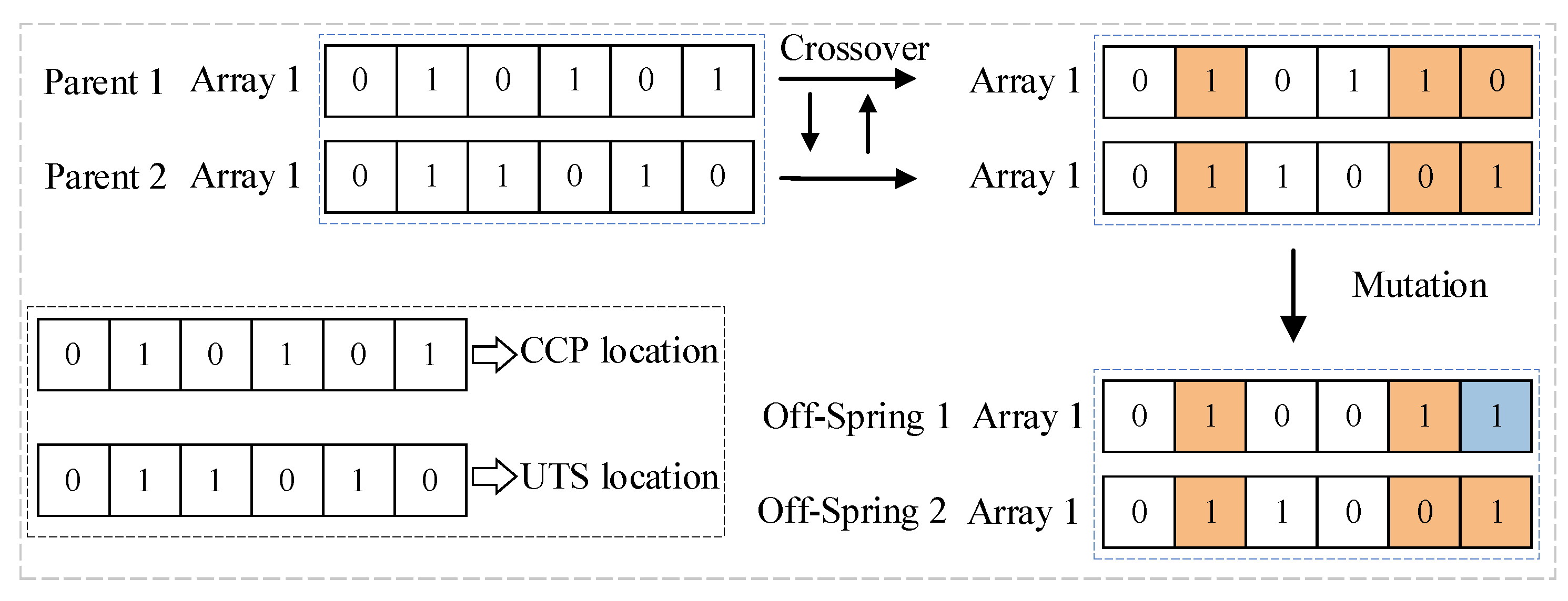
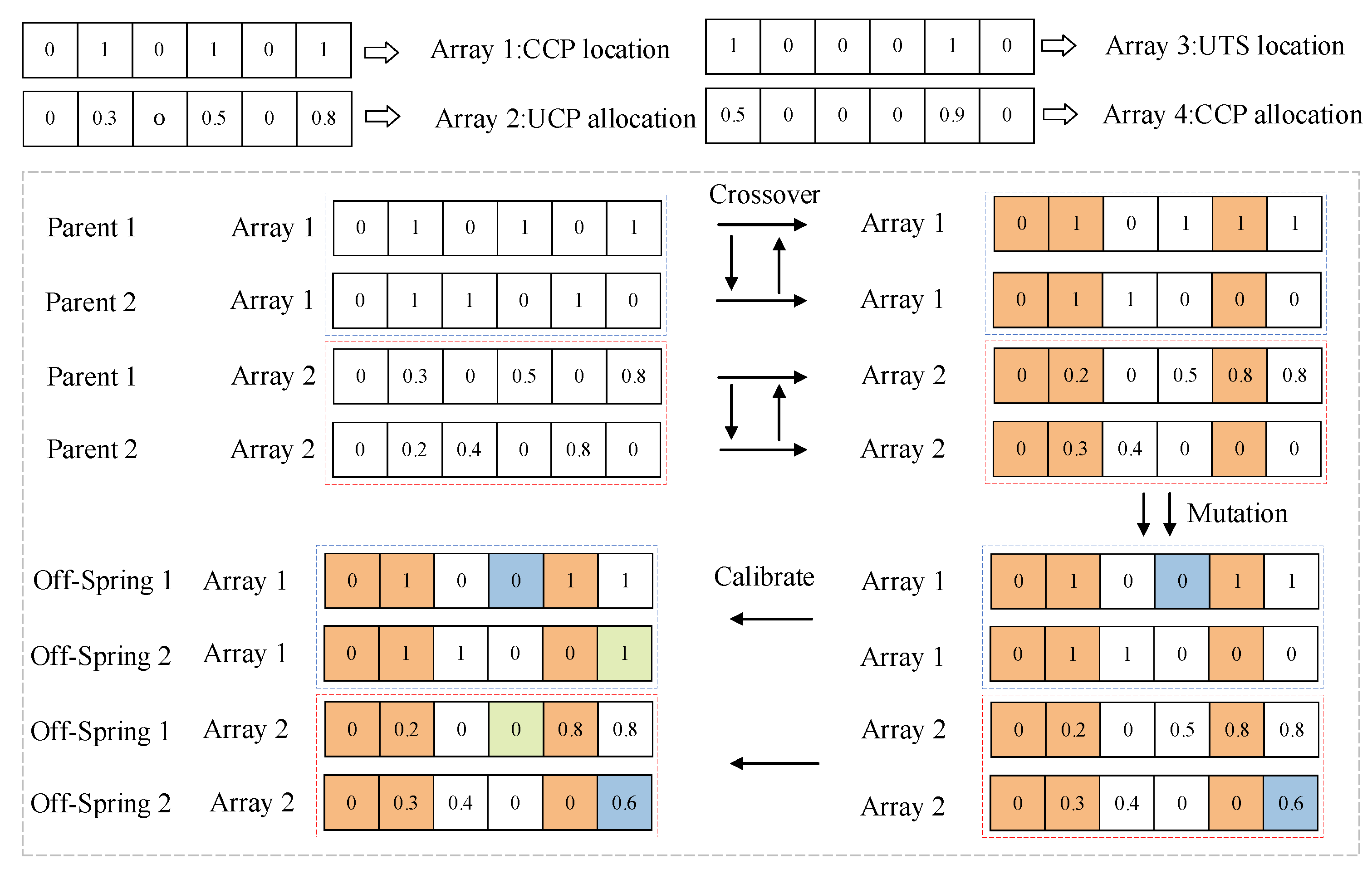
5.2.2. Genetic Operations
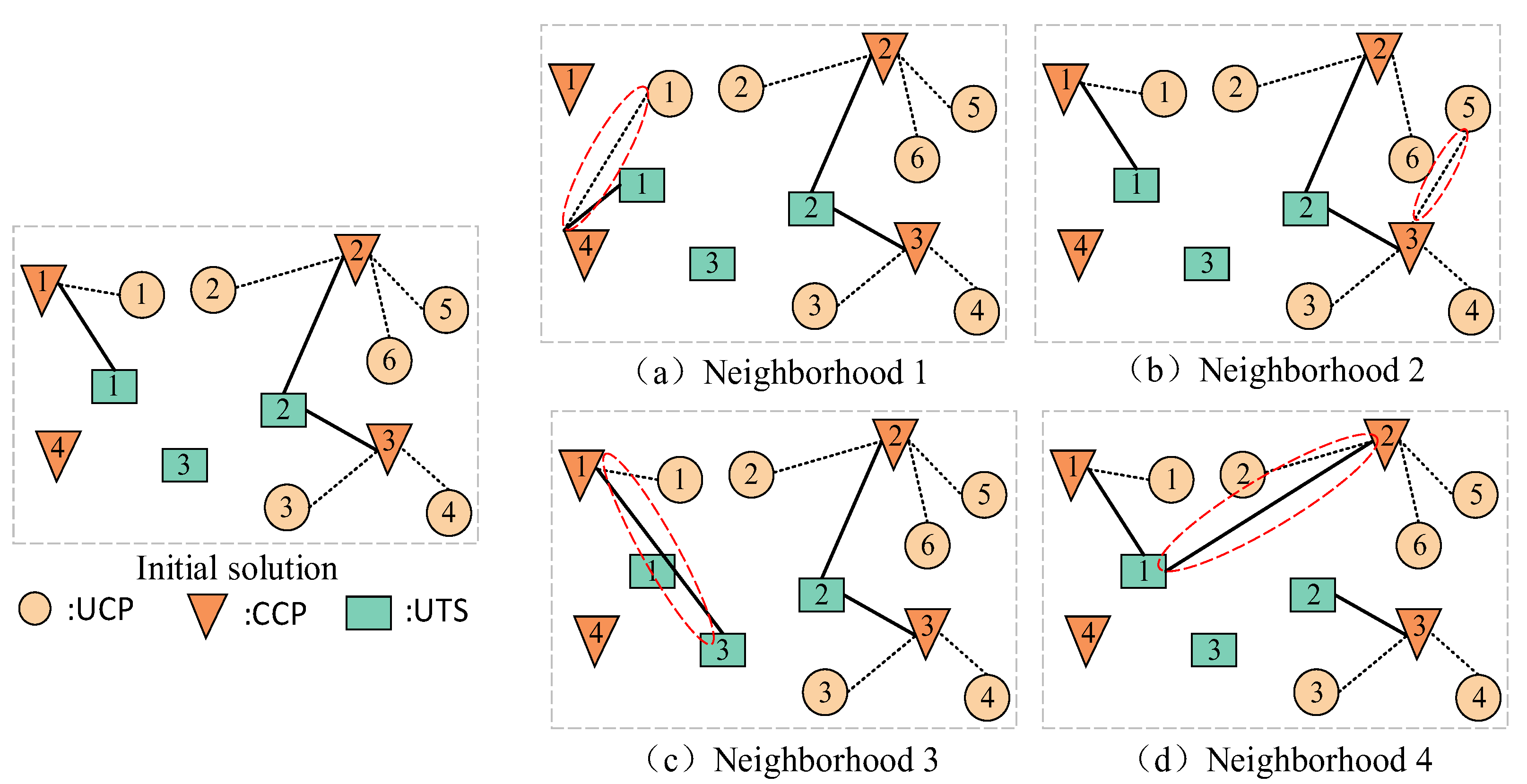
Use the four-dollar championship method to select the best individuals from the old population Ps, and obtain the next generation of Pa. The four-dollar championship method is to randomly select four individuals from the population, calculate the individual’s fitness value, and select the individual with the best fitness value to enter the next generation’s population.
Crossover operations. This paper adopts a shuffle-crossover strategy. For each crossover operation, two groups of parent genes from CCPs and UTSs position sequences and allocation sequences are selected in parallel crossover based on random order and an alternative operator. In order to ensure the feasibility of each offspring generation after crossover, it is necessary to modify it to adjust the corresponding relationship of chromosomes in the two sequences.
Mutation operators. This paper adopts a Gaussian mutation strategy. For individuals of each chromosome, the genes in the sequence of CCPs and UTSs location and the assigned sequence will be randomly selected to replace the original gene values with a single random number from a normal distribution with mean μ and variance σ2. However, certain mutation operations may result in infeasible offspring. In this case, mutations will be bypassed until it can ensure that the network is feasible. The GVNS genetic operation is shown in Figure 4.

5.2.3. VNS

VNS defines N_k (S) and N_l (S) as the neighborhood structures for shaking and local search. Repeat the shaking and local search process until the standard stop is met [36]. Based on the characteristics of the location–allocation problem, we propose four different neighborhood structures. As shown in Figure 5.
Neighborhood 1: Exchange of two CCPs. For every CCP, its assignment is exchanged with that of an unselected CCP. As shown in Figure 5a. The value of this neighborhood structure is reflected in the full utilization of all CCPs, preventing the search process from neglecting the selection of some CCPs and falling into local optimality. Consequently, this enhances the diversity within the search for solutions.
Neighborhood 2: Assign a UCP to a different CCP. For every UCP, it is assigned to different CCPs. As shown in Figure 5b. The advantage of this local structure is evidenced by the manner in which the allocation of a UCP to a CCP spans across all CCPs until the pinnacle of optimization is attained. This, in turn, safeguards against oversight in the search procedure regarding the choice of UCPs, thereby preventing descent into a local optimum and safeguarding the integrity of the solution’s quality.
Neighborhood 3: Exchange of two UTSs. For every UTS, its assignment is exchanged with an unselected UTS. As shown in Figure 5c. The value of this neighborhood structure is reflected in the full utilization of all UTSs, preventing the selection of some UTSs from being neglected during the search process. This facilitates a more effective departure from local optima, ensuring the assurance of solution quality.
Neighborhood 4: Assign a CCP to a different UTS. For every CCP, it is assigned to different UTSs. As shown in Figure 5d. The worth of this neighborhood structure is embodied in the fact that the process of assigning a CCP to a UTS traverses all the UTSs until the optimal result is found, which enhances the global search capability of the algorithm by increasing the selection of CCPs to jump out of the local optimum.
The shaking operator will randomly generate a feasible neighbor solution based on the selected neighborhood, which plays an important role in avoiding local optimality, as described below. If Neighborhood 1(3) is chosen, a selected CCP (UTS) and an unselected CCP (UTS) are randomly generated, and then the allocation of these two nodes is exchanged. If Neighborhood 2 is chosen, a UCP is randomly generated, and a random CCP different from the UCP assignment is generated, then the UCP is assigned to the CCP. If Neighborhood 4 is chosen, a CCP is randomly generated, and a random UTS but different from the CCP assignment is generated, then the CCP is assigned to the UTS, as shown in Figure 6. The merit of the dithering operator lies in its capacity to augment the diversity of the search, transcending the confines of local optima. By broadening the search scope, it provides the objective function with the prospect of discovering a superior solution. This mechanism significantly fortifies the algorithm’s global search prowess, thereby elevating the quality of solutions.
The proposed local search operators have a computationally acceptable complexity when solving large-scale UWCS network instances. Table 3 depicts the formulas for calculation times in each operator or shaking operator optimization step. The overall time complexity can be represented as a cubic polynomial. Considering the network case adopted in Appendix B Table A1 and the algorithm parameters given in Section 6.3, the total computation magnitude of the VNS was 1011. Evidently, it will not cause an unaffordable calculation workload, even if the instance size is huge.

6. Case Study

In this section, the application and effectiveness of the model in a real city case are demonstrated through a series of computational experiments that have been encoded in MATLAB 2017a software.

6.1. Small-Sized Experiments

The model solution was first validated on a set of five small problem examples, involving 50 to 150 UCPs, 5 to 10 CCPs, 1 to 5 UTSs, and 4 different types of treatment plants. The initial data used for the numerical simulation, such as coordinates, waste volume, and cost and capacity parameters, were determined adaptively. Population size and generations were set at 200 and 100, respectively. A reconstructed MILP model was developed to incorporate the aforementioned simplification steps and network principles. Each instance was solved by the GGA-VNS and CPLEX solvers.
Appendix B Table A2 shows that the solutions obtained by GGA-VNS differ slightly from the global optimality in network configuration (e.g., construction cost, transportation cost, procurement cost, etc.), but as the number of UCPs, CCPs, and UTSs increases, the solutions gradually become fully consistent with the global optimality. In terms of computational efficiency, although CPLEX solved very small instances faster, GGA-GVNS showed advantages in some relatively large instances. The CPU time of the CPLEX increased exponentially with the growth of the network. In contrast, the trend of increasing CPU time has proven to be much slower when using GGA-VNS. The experimental results reveal that the proposed solution method is sufficient to solve the UWCS location–allocation problem with good optimality and much less CPU time.

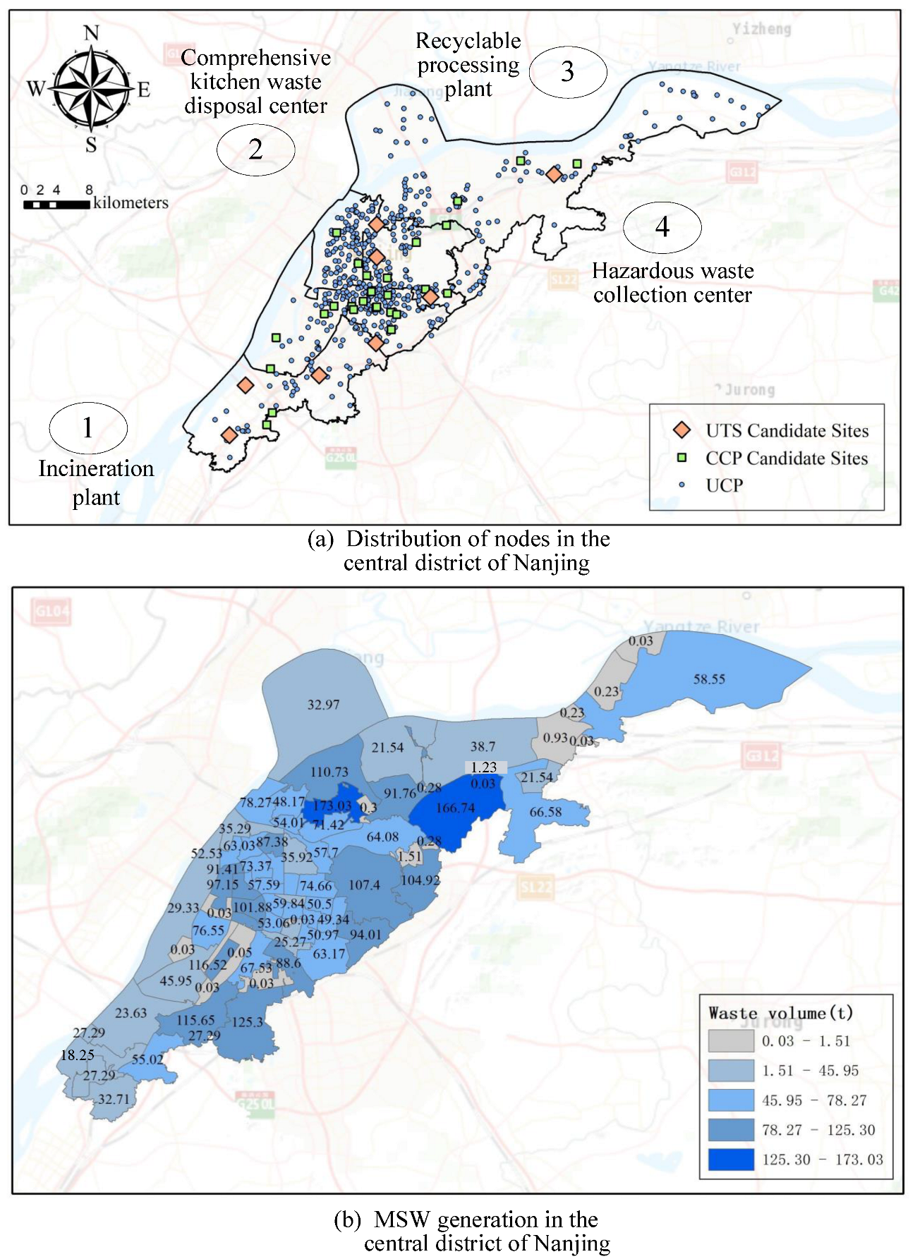
6.2. Background and Data

According to statistics, the resident population of Nanjing, China, will be 9.4 million in 2021, of which the population in the central district will account for about 46%. The central district generates about 50% of the total annual MSW in Nanjing (Nanjing Statistical Yearbook) and shows a steady increase in the average daily MSW generation rate over the years. For example, the increase from 0.63 kg/person in 2010 to 1.056 kg/person in 2020 is mainly due to population growth and increasing urbanization levels. The central district of Nanjing includes 7 of the 11 municipal districts of Nanjing, located in the middle of the city. According to the census in 2021, the area of the central district is about 787 square kilometers, and the population is about 4.32 million people. It can be seen that the small area and large population of the central district area bring with them a large amount of MSW generation, which seriously threatens the sustainable development of Nanjing.
In this study, in order to describe the reality of waste generation in the central district, the central location of each community within the central district is used as the demand point. Based on Baidu map data and ArcGIS 10.7 software, we have built a case summary of the UWCS network design in the central district. Figure 7a shows the locations of residential community points (i.e., UCPs) and the four types of treatment plants within the central district. A total of 445 UCPs were obtained through clustering and merging communities; treatment plants are outside the city, and locations are known. Figure 7b shows the amount of MSW generated by each street in the central district.
It is well known that MSW generation is closely related to population [51]. According to the Nanjing Statistical Yearbook, the total population of Nanjing and MSW clearing volume can be obtained for each year from 2015 to 2020. Using Equation (22), we can obtain the per capita daily generation in each year and finally weigh the data to obtain a more accurate per capita daily generation in Nanjing of about 0.88 kg (a constant value). The population of each demand point in Nanjing is known (based on the seventh census), multiplied by the per capita daily generation, and the daily generation of MSW at each demand point is obtained.
q = R 365 Q
We consulted experts in the field of waste management and learned from the Nanjing Urban Management Bureau to understand the production of various types of waste in Nanjing MSW. On this basis, the proportion of MSW is derived as 55% for kitchen waste, 22% for recyclable waste, 18% for other waste, 1% for hazardous waste, and 4% for bulky waste, whereas in UTS-MSW, bulky waste is not considered, and its traditional transportation method is still used.
We have adjusted the parameter values used for the simulation based on the available techniques, local standards, and expert surveys, as shown in Table 4. These parameters ensure that the simulation output of our model has strong consistency with the actual project cases.

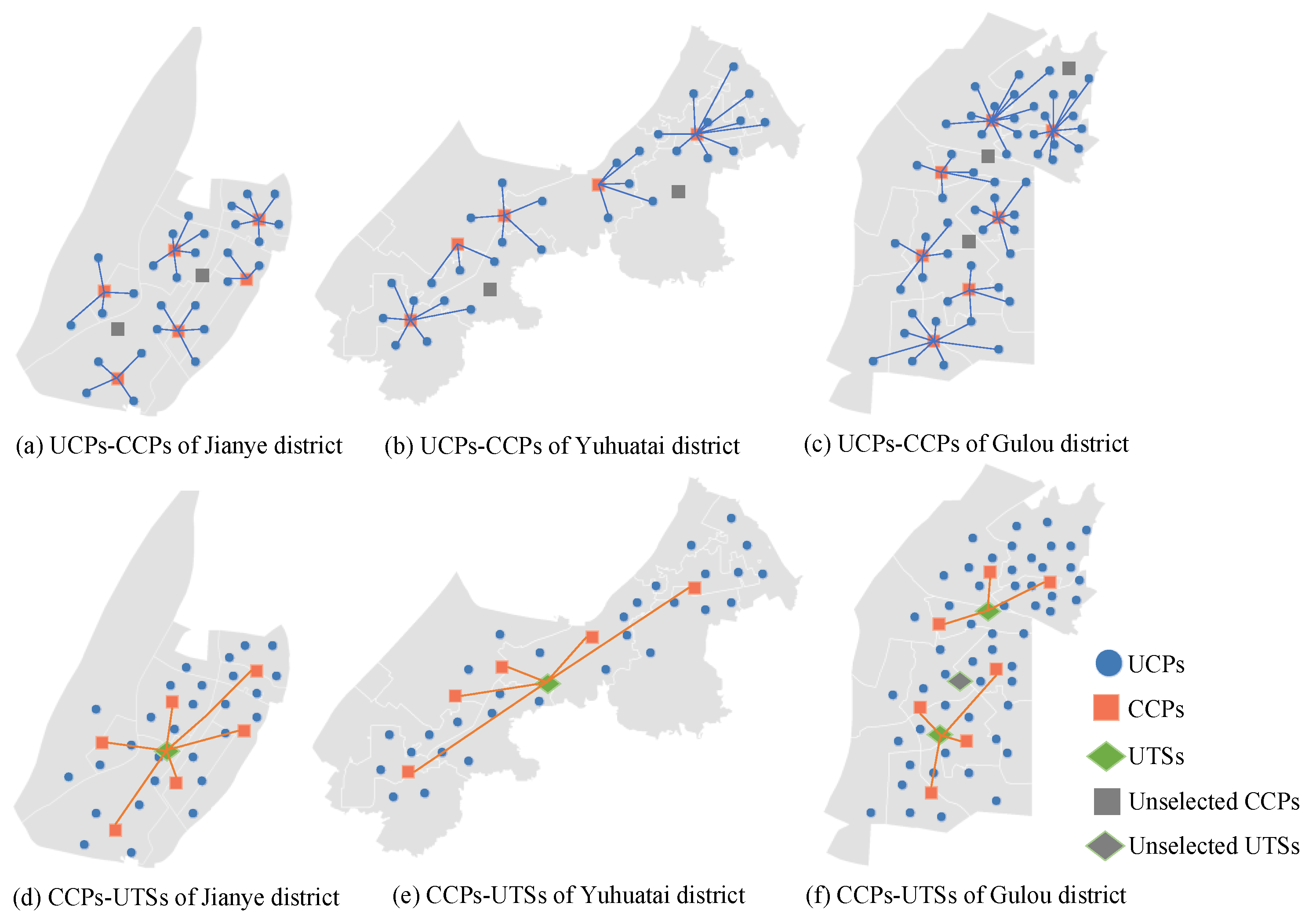
6.3. Results Analysis

We have conducted several simulations for the central city case of Nanjing, and the results show that the proposed hybrid optimization algorithm spends an average of 490.2043 s CPU time per run to obtain the optimal solution of the location–allocation model. Such calculations take little time and ensure the advantages of our model in realistic decision-making.
With the settings of p1 = 27, p2 = 8, and p3 = 3 (according to the capacity of the facility and the actual situation), we obtained the optimal network layout after simulation, as shown in Figure 8. Among them, the best network configuration between the UWCS is shown in Table 5.
The results show that a total of 19 nodes were selected from the CCP candidate nodes, and 4 nodes were selected from the UTS candidate nodes. The construction cost is about 3.5 × 10⁵ dollars per day, of which the construction cost of CCPs and UTSs is about 4.9 × 10⁴ dollars per day and 4.8 × 10⁴ dollars per day, accounting for 13.92% and 13.74%, respectively, and the remaining pipeline construction cost reaches 72.34%. The purchase cost is about 170 dollars per day, and the total number of equipment purchases is about 47. The transportation cost is about 1.6 × 10⁵ dollars per day, and the total cost is about 5.1 × 10⁵ dollars per day. It can be seen that the proportion of construction costs in total costs is large, reaching 68.56%, and the procurement cost accounts for the smallest, only 0.03% of the total cost. This is because in underground construction, the difficulty and complexity of the geology lead to a large cost of construction, while procurement costs include only equipment purchases at CCPs and therefore account for the smallest percentage.
According to Equations (19) and (20), the two types of benefits generated by the UWCS network reached 5.3408 × 10⁶ dollars per year, which means that the UWCS network saves 5.34 × 10⁶ dollars per year in land conservation compared to conventional collection systems. After two decades of operations, the UWCS has generated a total of 1.6 × 10⁵ dollars in environmental benefits from reduced carbon, NOx, and PM emissions, as well as reduced water pollutants, reduced noise, and conservation of non-renewable energy. Through statistical analysis, it can be clearly seen that as the operating time increases, the advantages of UWCS in land conservation and environmental benefits are still optimistic.

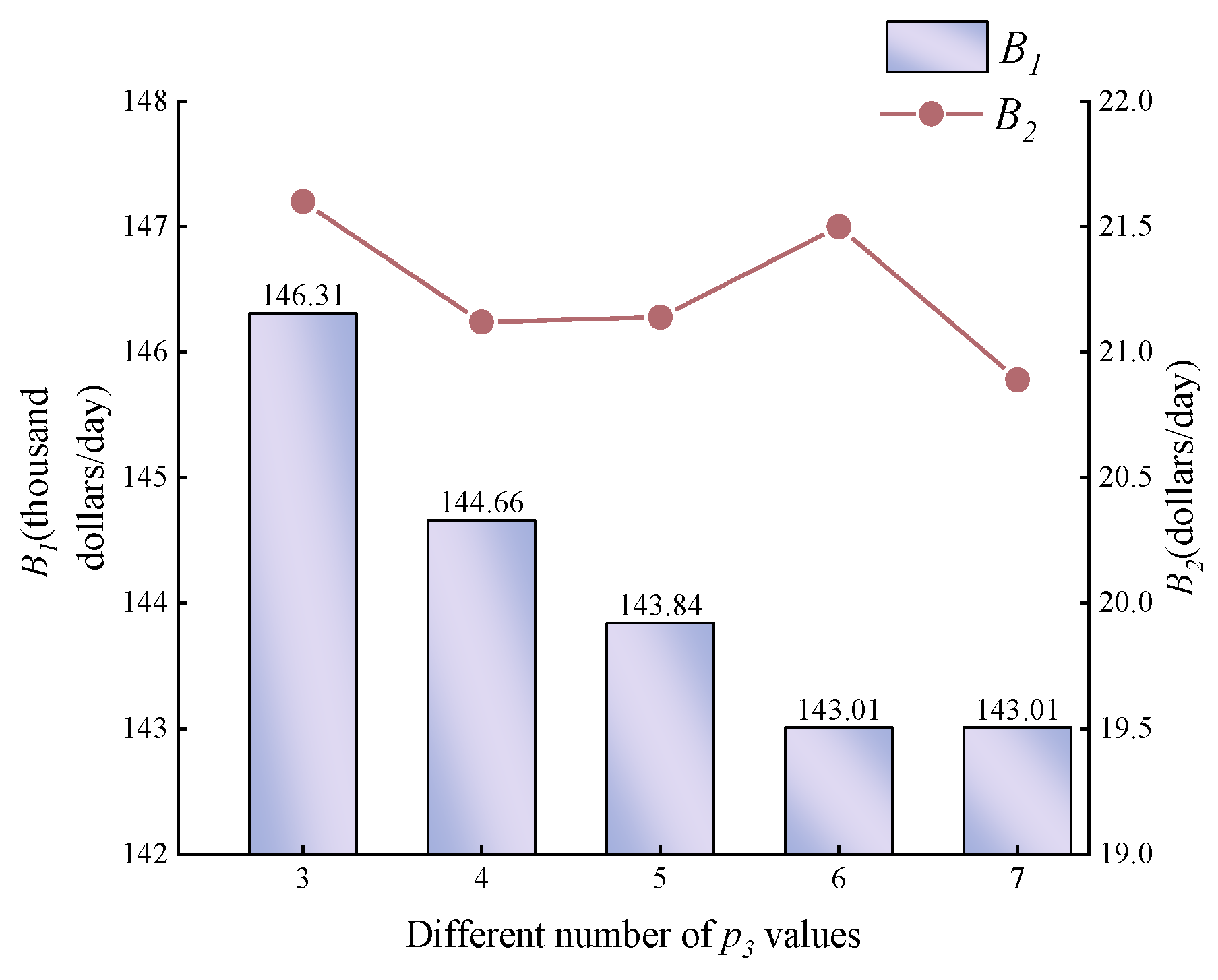
6.4. Sensitivity Analysis

Considering the uncertainty of the device placed in CCPs in the actual UWCS decision, analyze the sensitivity of the objective costs, network configurations, and benefits by changing the value of p3. Sensitivity was tested under several representative scenarios and then compared with p3 = 3 as the baseline result.
After simulation, the network configuration can be obtained in different situations of p3, including the number of CCPs and UTSs, target costs, benefits, and total devices. Among them, p3 values are set for five scenarios. The results showed that as p3 increased, the number of total devices kept increasing, and the number of selected CCPs decreased accordingly, while the number of UTSs remained constant. This is because the number of devices allowed to be installed is increasing, the processing capacity of each CCP is growing, and the number of its chosen continues to decrease. The choice of UTSs has nothing to do with the value of p3.
Figure 9a–d illustrate the relationship between the objective cost and p3. Obviously, with the increase in p3, construction and transportation costs decrease, while procurement costs increase. This is because the number of configuration devices allowed in each CCP will lead to a decrease in the number of CCPs constructed, thereby reducing the transportation distance of waste flow. The construction cost and transportation cost have been reduced accordingly. Of course, as the installation equipment increases, the required procurement cost will increase accordingly, but the procurement cost only accounts for 0.03% of the total cost, which has a small impact on the total cost. Therefore, under the premise of determining the capacity of CCPs and the processing capacity of the secondary pipelines, the number of facilities at CCPs should be reduced as much as possible to reduce investment in the total system network.
Figure 10 illustrates the relationship between benefits and p3. Obviously, the land benefit and the environmental benefit are in a synchronous dynamic change with the increase of the p3 value. This is because the land benefit is related to the number of CCPs and UTSs selected, and the environmental benefit is related to the transport MSW stream parameters. During the change in the value of p3, while the number of selected UTSs is unchanged, the number of selected CCPs decreases continuously, the transport distance changes, and the waste flow of transportation among facilities will also change accordingly. Therefore, from the perspective of UWCS, there is the best combination of benefits between p3 values and two types of benefits.
Based on the sensitivity analysis and evaluation, some managerial insights for UWCS decision-making are disclosed.
(1)
Due to the disparate distribution of geography and waste volumes, the utilization rate of nodes and pipelines in various urban sectors may exhibit substantial disparities, thereby diminishing the economies of scale impact of the Underground Waste Collection System (UWCS). As cities progress and UWCS implementation unfolds, it becomes imperative for the government to provide policy support for subterranean transportation, thereby nurturing an optimal environment for the design of the UWCS network.
(2)
From an external perspective, the networked development of UWCS can bring significant social and environmental benefits, along with advantages from automated operations and economies of scale. It is anticipated that the advantages ushered in by UWCS at this juncture can significantly diminish the government’s financial outlay on the management, operation, and maintenance of MSW.
(3)
From the perspective of urban development, UWCS emerges as a potent strategy for propelling sustainable aspirations. By seamlessly melding a specialized subterranean infrastructure network, the management of MSW and subterranean transportation coalesce synergistically into a cohesive system committed to intelligent and sustainable MSW management endeavors. The automated categorization of MSW and the provision of real-time information updates during transportation confer considerable convenience upon residents in waste disposal, concurrently refining MSW management operations for governmental authorities.

7. Conclusions and Future Research

This paper addresses the UWCS network design problem. By analyzing the limitations of the current MSW transportation system, the whole process of operation in the underground was designed based on an intelligent technical system. First, the importance of demand points was evaluated using the E-Topsis evaluation method to obtain candidate nodes for CCPs and UTSs. Then, an MILP model was formulated by considering minimum total cost, and a GGA-GVNS hybrid optimization algorithm was developed to simplify the model and obtain the optimal solution to the problem (i.e., node location–allocation, pipeline layout, and waste flow). Finally, a case study based on the central city of Nanjing was conducted to validate the proposed model and solution technique in different scenarios. The experimental results show that the GGA-GVNS algorithm has strong efficiency in this model. Therefore, under the premise of reasonable planning, our suggested UWCS proves to be both practical and viable.
Through a meticulous exploration of the UWCS network in Nanjing, we summarize the following implications regarding practical and theoretical aspects. On the theoretical front, this study proposes an automated, large-scale underground collection system for MSW. Simultaneously, it conducts a systematic study on the whole set of operation flows in the system, including waste categorization, facility siting, pipeline transportation capacity, and the hierarchical interplay among facilities. In conjunction with the practical context, a network planning model for UWCS is built. Furthermore, by designing the corresponding intelligent solution algorithms to obtain the optimal layout of the multi-class facility network and the optimal layout of facility siting. This set of methods can establish a robust theoretical foundation for MSW underground collection systems and other forms of urban underground systems in future smart city planning, management, and construction. In practice, the UWCS can help cities establish a comprehensive and efficient waste logistics network system. At the same time, it assumes practical and guiding significance in the pursuit of constructing resource-efficient and environmentally friendly modernized urban landscapes. It presents a novel perspective for contemplating the sustainable development of cities and the harnessing of underground spaces.
This study provides a new planning concept for the planning and management of UWCS. However, some limitations still exist. Moreover, due to the unavailability of exact data, we attached strict assumptions, which may reduce the applicability of our model in UWCS network design. The system we designed did not address the problems of MSW transport fleet scheduling. Future research can be carried out in two aspects. Firstly, consider the dynamics of MSW underground networks, such as the uncertain waste amount, the modeling of waste generation amount, and the scheduling of operating vehicles [31,56,57]. Secondly, considering the cities’ sustainable development goals, we should pay more attention to the strategic level of network planning, such as the construction scale of underground networks and how to achieve the coordinated operation of the UWCS and traditional highway transportation systems.

Author Contributions

Conceptualization, J.D.; methodology, Q.L. and Y.C.; software, W.H.; validation, B.S. and H.C.; writing—original draft preparation, Q.L.; writing—review and editing, W.H. and Y.C.; visualization, B.S.; funding acquisition, J.D. All authors have read and agreed to the published version of the manuscript.

Funding

This work was supported in part by the National Natural Science Foundation of China under Grants 52102392, 72271125 and 71971214.

Data Availability Statement

The data presented in this study are available on request from the corresponding author.

Conflicts of Interest

The authors declare no conflict of interest.

Appendix A. E-Topsis Computational Procedures

Notice: This part of the parameter has nothing to do with the parameter in Section 4 above, and it is just an introduction to the computational steps of the TOPSIS approach.
Step 1: Construct the original evaluation index matrix. Assuming that there are n evaluation indicators and m demand points to choose from, the value of indicator i in subset j is aij, the original decision matrix A consisting of the indicator data for the m demand points.
A = a i j m n = a 11 a 1 n a m 1 a m n
Step 2: Generate a standardized matrix. Standardize the data in matrix A, the calculation formula is as follows.
For positive indicators:
z i j = a i j min a i j max a i j min a i j
For negative indicators:
z i j = max a i j a i j max a i j min a i j
After standardization of the data, the standard matrix after the original data is naturalized, and it is recorded as Z:
Z = z i j z 1 n z m 1 z m n
Step 3: Determine the index weight. Firstly, calculate the weight of evaluation demand point i under the j indicator for that indicator Pij, Ej represents the entropy value of the j indicator, and Wj represents the weight of each indicator.
P i j = z i j i = 1 m z i j E j = 1 ln m i = 1 m P i j ln P i j , j = 1 , 2 , , n w j = 1 E j j = 1 n 1 E j
Step 4: Generate evaluation matrix R.
R = r i j m n = w j z i j m n = w 1 z 11 w j z 1 n w 1 z m 1 w j z m n = r 11 r 1 n r m 1 r m n
Step 5: Determine the ideal solution V+ and the negative ideal solution V. After obtaining the evaluation matrix, it is necessary to determine the positive ideal solution V+ and the negative ideal solution V. The calculation formula is as follows.
V + = r 1 + , , r j + , , r n + V = r 1 , , r j , , r n
among them, r j + = max r i j | 1 i m , r j = min r i j | 1 i m .
Step 6: Calculate the distance. Calculate the distance di+ from each evaluation vector to the positive ideal solution and the distance di from the negative ideal solution, respectively. Using the European distance calculations di+ and di [42], the formula is as follows.
d i + = j = 1 n w j ( r j + r i j ) 2 1 2 , i = 1 , 2 , 3 , , m d i = j = 1 n w j r j + r i j 2 1 2 , i = 1 , 2 , 3 , m
Step 7: Calculation sticker progress ci for sorting.
c i = d i d i + + d i , i = 1 , 2 , 3 , m
ci indicates the relative closeness of the evaluation demand point i to the ideal solution. The range of the value is between 0 and 1. The closer the value is to 1, the closer the value of the positive ideal, the more important the demand point is.

Appendix B

Table A1. Number of variables and constraints in the UWCS network model.
Variables ConstraintsNumber at MostCase
Variables xj, ym, ηj2 × |J| + |M|62
Variables Zij, Sjm|I| • |J| + |J| • |M|12,231
Variables Zij, Sjm, Wmnu, Qiju, Pmnu, Rmnu2 × |U| • |M| • |N| + |U| • |I| • |J|+|U| • |J| • |M|49,180
Cons. (5), (11), (13), (14), (16), (17)|I| + 7 × |I| + 5 × |M|674
Cons. (6), (7), (8), (9), (18)|I| • |J| • (|U| + 2)72,090
Cons. (10), (12), (19), (23)3 × |J| • |M| + 2650
Cons. (15), (20), (21), (22), (24), (25)2 × |J| + |M| + |I| • |J| • (3 × |U| + 1) + |J| • |M| • (3 × |U| + 1) + 4 × |U| • |M| • |N|159,577
All/294,464
Table A2. Comparison of GGA-GVNS and CPLEX on small-sized instances.
NoHypothetical Instancep1, p2, p3ApproachF1F2F3FCPU Time (s)Gap (%)
150 UCPs, 3 CCPs, 2 UTSs2, 1, 1GGA-GVNS69.11900.007119.622688.748823.30450.0%
CPLEX69.11500.007119.621988.74400.4600
250 UCPs, 5 CCPs, 3 UTSs5, 3, 2GGA-GVNS66.45270.007119.442785.902522.83150.3%
CPLEX66.66350.007119.504486.17500.4800
3100 UCPs, 5 CCPs, 3 UTSs5, 3, 2GGA-GVNS130.44970.014237.1766167.640633.39041.2%
CPLEX132.06550.014237.6373169.717014.4300
4100 UCPs, 10 CCPs, 5 UTSs10, 5, 3GGA-GVNS71.83080.014237.4301109.275235.50500.0%
CPLEX71.83010.014237.4297109.274047.7300
5150 UCPs, 10 CCPs, 5 UTSs10, 5, 3GGA-GVNS85.09390.014265.0640150.172145.72440.0%
CPLEX85.09330.014265.0635150.171080.34000.0%
Table A3. Nomenclature of system components.
Nomenclature of System Components
UWCSunderground waste collection system
MSW municipal solid waste
KWkitchen waste
OWother waste
RWrecyclable waste
HWhazardous waste
UCPunderground collection point
CCPconcentrated collection point
UTSunderground transfer station
CKWDCkitchen waste disposal center
IPincineration plant
RPPrecyclable processing plant
HWCChazardous waste collection center
TP-1, TP-2, TP-3third-level pipelines (three types)
SPsecond-level pipeline
FPfirst-level pipeline

References

  1. Farre, J.A.; Salgado-Pizarro, R.; Martin, M.; Zsembinszki, G.; Gasia, J.; Cabeza, L.F.; Barreneche, C.; Fernandez, A.I. Case study of pipeline failure analysis from two automated vacuum collection system. Waste Manag. 2021, 126, 643–651. [Google Scholar] [CrossRef]
  2. Khan, A.H.; Lopez-Maldonado, E.A.; Khan, N.A.; Villarreal-Gomez, L.J.; Munshi, F.M.; Alsabhan, A.H.; Perveen, K. Current solid waste management strategies and energy recovery in developing countries—State of art review. Chemosphere 2021, 291, 133088. [Google Scholar] [CrossRef] [PubMed]
  3. Sajid, M.; Raheem, A.; Ullah, N.; Asim, M.; Ur Rehman, M.S.; Ali, N. Gasification of municipal solid waste: Progress, challenges, and prospects. Renew. Sust. Energ. Rev. 2022, 168, 112815. [Google Scholar] [CrossRef]
  4. Saadatlu, E.A.; Barzinpour, F.; Yaghoubi, S. A sustainable model for municipal solid waste system considering global warming potential impact: A case study. Comput. Ind. Eng. 2022, 169, 108127. [Google Scholar] [CrossRef]
  5. Lino, F.A.; Ismail, K.A.; Castañeda-Ayarza, J.A. Municipal solid waste treatment in Brazil: A comprehensive review. Energy Nexus 2023, 11, 2772–4271. [Google Scholar] [CrossRef]
  6. Zhang, L.; Liu, Z.; Shan, W.; Yu, B. A stabilized branch-and-price-and-cut algorithm for the waste transportation problem with split transportation. Comput. Ind. Eng. 2023, 178, 109143. [Google Scholar] [CrossRef]
  7. Ding, Y.; Zhao, J.; Liu, J.-W.; Zhou, J.; Cheng, L.; Zhao, J.; Shao, Z.; Iris, Ç.; Pan, B.; Li, X.; et al. A review of China’s municipal solid waste (MSW) and comparison with international regions: Management and technologies in treatment and resource utilization. J. Clean Prod. 2021, 293, 126144. [Google Scholar] [CrossRef]
  8. Xiao, W.; Liu, T.; Tong, X. Assessing the carbon reduction potential of municipal solid waste management transition: Effects of incineration, technology and sorting in Chinese cities. Resour. Conserv. Recycl. 2023, 188, 106713. [Google Scholar] [CrossRef]
  9. Guo, S.; Chen, L. Why is China struggling with waste classification? A stakeholder theory perspective. Resour. Conserv. Recycl. 2022, 183, 106312. [Google Scholar] [CrossRef]
  10. Rathore, P.; Sarmah, S.P. Modeling transfer station locations considering source separation of solid waste in urban centers: A case study of Bilaspur city, India. J. Clean. Prod. 2019, 211, 44–60. [Google Scholar] [CrossRef]
  11. Wang, Y.; Shou, R.; Lee, L.H.; Chew, E.P. A case study on sample average approximation method for stochastic supply chain network design problem. Front. Eng. Manag. 2017, 4, 338–347. [Google Scholar] [CrossRef]
  12. Miller, B.; Spertus, J.; Kamga, C. Costs and benefits of pneumatic collection in three specific New York City cases. Waste Manag. 2014, 34, 1957–1966. [Google Scholar] [CrossRef] [PubMed]
  13. Hu, W.; Dong, J.; Hwang, B.-G.; Ren, R.; Chen, Z. Hybrid optimization procedures applying for two-echelon urban underground logistics network planning: A case study of Beijing. Comput. Ind. Eng. 2020, 144, 106452. [Google Scholar] [CrossRef]
  14. Hu, W.; Dong, J.; Xu, N. Multi-period planning of integrated underground logistics system network for automated construction-demolition-municipal waste collection and parcel delivery: A case study. J. Clean. Prod. 2022, 330, 129760. [Google Scholar] [CrossRef]
  15. Popa, C.; Carutasu, G.; Cotet, C.; Carutasu, N.; Dobrescu, T. Smart City Platform Development for an Automated Waste Collection System. Sustainability 2017, 9, 2064. [Google Scholar] [CrossRef]
  16. Fen, B.; Ye, Q. Operations management of smart logistics: A literature review and future research. Front. Eng. Manag. 2020, 8, 344–355. [Google Scholar] [CrossRef]
  17. Jiang, Z.Z.; Feng, G.; Yi, Z.; Guo, X. Service-oriented manufacturing_ A literature review and future research directions. Front. Eng. Manag. 2022, 9, 71–88. [Google Scholar] [CrossRef]
  18. Chàfer, M.; Sole-Mauri, F.; Solé, A.; Boer, D.; Cabeza, L.F. Life cycle assessment (LCA) of a pneumatic municipal waste collection system compared to traditional truck collection. Sensitivity study of the influence of the energy source. J. Clean. Prod. 2019, 231, 1122–1135. [Google Scholar] [CrossRef]
  19. Hidalgo, D.; Martín-Marroquín, J.M.; Corona, F.; Juaristi, J.L. Sustainable vacuum waste collection systems in areas of difficult access. Tun. Under Space Technol. 2018, 81, 221–227. [Google Scholar] [CrossRef]
  20. Nakou, D.; Benardos, A.; Kaliampakos, D. Assessing the financial and environmental performance of underground automated vacuum waste collection systems. Tun. Under. Space Technol. 2014, 41, 263–271. [Google Scholar] [CrossRef]
  21. Jiawei, M.; Han, Y.; Li, L.; Liu, J. Distribution characteristics and potential risks of bacterial aerosol in waste transfer station. J Environ. Manag. 2023, 326, 116599. [Google Scholar] [CrossRef] [PubMed]
  22. Son Le, H.; Louati, A. Modeling municipal solid waste collection: A generalized vehicle routing model with multiple transfer stations, gather sites and inhomogeneous vehicles in time windows. Waste Manag. 2016, 52, 34–49. [Google Scholar] [CrossRef] [PubMed]
  23. Ye, Q.; Umer, Q.; Zhou, R.; Asmi, A.; Asmi, F. How publications and patents are contributing to the development of municipal solid waste management: Viewing the UN Sustainable Development Goals as ground zero. J. Environ. Manag. 2023, 325, 116496. [Google Scholar] [CrossRef] [PubMed]
  24. Pouriani, S.; Asadi-Gangraj, E.; Paydar, M.M. A robust bi-level optimization modelling approach for municipal solid waste management; a real case study of Iran. J. Clean Prod. 2019, 240, 118125. [Google Scholar] [CrossRef]
  25. Riaz, M.; Farid, H.M.A. Enhancing Green Supply Chain Efficiency Through Linear Diophantine Fuzzy Soft-Max Aggregation Operators. J. Ind. Intell. 2023, 1, 8–29. [Google Scholar] [CrossRef]
  26. Wu, T.-W.; Zhang, H.; Peng, W.; Lv, F.; He, P.-J. Applications of convolutional neural networks for intelligent waste identification and recycling: A review. J. Environ. Manag. 2023, 190, 106813. [Google Scholar] [CrossRef]
  27. Fernández, C.; Manyà, F.; Mateu, C.; Sole-Mauri, F. Approximate dynamic programming for automated vacuum waste collection systems. Environ. Modell. Soft. 2015, 67, 128–137. [Google Scholar] [CrossRef]
  28. Li, H.Q.; Fan, Y.Q.; Yu, M.J. Deep Shanghai project—A strategy of infrastructure integration for megacities. Tun. Under. Space Technol. 2018, 81, 547–567. [Google Scholar] [CrossRef]
  29. Tsydenova, N.; Becker, T.; Walther, G. Optimized design of concrete recycling networks: The case of North Rhine-Westphalia. Waste Manag. 2021, 135, 309–317. [Google Scholar] [CrossRef]
  30. Oyola-Cervantes, J.; Amaya-Mier, R. Reverse logistics network design for large off-the-road scrap tires from mining sites with a single shredding resource scheduling application. Waste Manag. 2019, 100, 219–229. [Google Scholar] [CrossRef]
  31. Trochu, J.; Chaabane, A.; Ouhimmou, M. A two-stage stochastic optimization model for reverse logistics network design under dynamic suppliers’ locations. Waste Manag. 2019, 95, 569–583. [Google Scholar] [CrossRef] [PubMed]
  32. Govindan, K.; Nosrati-Abarghooee, S.; Nasiri, M.M.; Jolai, F. Green reverse logistics network design for medical waste management: A circular economy transition through case approach. J. Environ. Manag. 2022, 322, 115888. [Google Scholar] [CrossRef]
  33. Yousefloo, A.; Babazadeh, R.; Mohammadi, M.; Pirayesh, A.; Dolgui, A. Design of a robust waste recycling network integrating social and environmental pillars of sustainability. Comput. Ind. Eng. 2023, 176, 108970. [Google Scholar] [CrossRef]
  34. Blazquez, C.; Paredes-Belmar, G. Network design of a household waste collection system: A case study of the commune of Renca in Santiago, Chile. Waste Manag. 2020, 116, 179–189. [Google Scholar] [CrossRef] [PubMed]
  35. Lu, X.; Pu, X.; Han, X. Sustainable smart waste classification and collection system: A bi-objective modeling and optimization approach. J. Clean. Prod. 2020, 276, 124183. [Google Scholar] [CrossRef]
  36. Shang, X.; Yang, K.; Jia, B.; Gao, Z. The stochastic multi-modal hub location problem with direct link strategy and multiple capacity levels for cargo delivery systems. Transp. A Transp. Sci. 2020, 17, 380–410. [Google Scholar] [CrossRef]
  37. Hashemi-Amiri, O.; Mohammadi, M.; Rahmanifar, G.; Hajiaghaei-Keshteli, M.; Fusco, G.; Colombaroni, C. An allocation-routing optimization model for integrated solid waste management. Expert Syst. Appl. 2023, 227, 0957–4174. [Google Scholar] [CrossRef]
  38. Enevo. 2022. Available online: https://enevo.com/ (accessed on 12 July 2022).
  39. Envac. 2022. Available online: https://cleanrobotics.com/ (accessed on 12 July 2022).
  40. Zhao, L.; Zhou, J.; Li, H.; Yang, P.; Zhou, L. Optimizing the design of an intra-city metro logistics system based on a hub-and-spoke network model. Tun. Under. Space Technol. 2021, 116, 104086. [Google Scholar] [CrossRef]
  41. Dai, L.; Wang, J. Evaluation of the Profitability of Power Listed Companies Based on Entropy Improved TOPSIS Method. Procedia Eng. 2011, 15, 4728–4732. [Google Scholar] [CrossRef]
  42. Eftihia Nathanaila, G.A.M.G. A novel approach for assessing sustainable city logistics. Transp. Res. Procedia 2016, 25, 1036–1045. [Google Scholar] [CrossRef]
  43. Sengupta, D.; Das, A.; Bera, U.K. A sustainable green reverse logistics plan for plastic solid waste management using TOPSIS method. Environ. Sci. Pollut Res. 2023, 30, 97734–97753. [Google Scholar] [CrossRef] [PubMed]
  44. Sagnak, M.; Berberoglu, Y.; Memis, I.; Yazgan, O. Sustainable collection center location selection in emerging economy for electronic waste with fuzzy Best-Worst and fuzzy TOPSIS. Waste Manag. 2021, 127, 37–47. [Google Scholar] [CrossRef] [PubMed]
  45. Petrović, N.; Živojinović, T.; Mihajlović, J. Evaluating the Annual Operational Efficiency of Passenger and Freight Road Transport in Serbia Through Entropy and TOPSIS Methods. J. Eng. Manag. Syst. Eng. 2023, 2, 204–211. [Google Scholar] [CrossRef]
  46. Dong, J.; Hu, W.; Yan, S.; Ren, R.; Zhao, X. Network Planning Method for Capacitated Metro-Based Underground Logistics System. Adv. Civ. Eng. 2018, 2018, 6958086. [Google Scholar] [CrossRef]
  47. Hu, W.; Dong, J.; Ren, R.; Chen, Z. Underground logistics systems: Development overview and new prospects in China. Front. Eng. Manag. 2023, 10, 354–359. [Google Scholar] [CrossRef]
  48. Hu, W.; Dong, J.; Yang, K.; Hwang, B.G.; Ren, R.; Chen, Z. Reliable design of urban surface-underground integrated logistics system network with stochastic demand and social-environmental concern. Comput. Ind. Eng. 2023, 181, 109331. [Google Scholar] [CrossRef]
  49. Hansen, N.; Mladenović, P. Variable neighborhood search. Comput. Oper. Res. 1997, 24, 1097–1100. [Google Scholar] [CrossRef]
  50. Dib, O.; Manier, M.-A.; Moalic, L.; Caminada, A. Combining VNS with Genetic Algorithm to solve the one-to-one routing issue in road networks. Comput. Oper. Res. 2017, 78, 420–430. [Google Scholar] [CrossRef]
  51. Lv, J.; Dong, H.; Geng, Y.; Li, H. Optimization of recyclable MSW recycling network: A Chinese case of Shanghai. Waste Manag. 2020, 102, 763–772. [Google Scholar] [CrossRef]
  52. Soni, A.R.; Chandel, M.K. Assessment of emission reduction potential of Mumbai metro rail. J. Clean. Prod. 2018, 197, 1579–1586. [Google Scholar] [CrossRef]
  53. Coulombel, N.; Dablanc, L.; Gardrat, M.; Koning, M. The environmental social cost of urban road freight: Evidence from the Paris region. Transp. Res. Part D Transp. Environ. 2018, 63, 514–532. [Google Scholar] [CrossRef]
  54. Hu, W.; Dong, J.; Hwang, B.G.; Ren, R.; Chen, Z. Network planning of urban underground logistics system with hub-and-spoke layout: Two phase cluster-based approach. Eng. Constr. Archit. Manag. 2020, 27, 2079–2105. [Google Scholar] [CrossRef]
  55. Roy, A.; Manna, A.; Kim, J.; Moon, I. IoT-based smart bin allocation and vehicle routing in solid waste management: A case study in South Korea. Comput. Ind. Eng. 2022, 171, 108457. [Google Scholar] [CrossRef]
  56. Tirkolaee, E.B.; Mahdavi, I.; Esfahani, M.M.S.; Weber, G.W. A robust green location-allocation-inventory problem to design an urban waste management system under uncertainty. Waste Manag. 2020, 102, 340–350. [Google Scholar] [CrossRef]
  57. Zhao, H.R.; Cao, Y.; Wang, X.; Li, B.K.; Wang, Y.W. Distributionally robust optimization for dispatching the integrated operation of rural multi-energy system and waste disposal facilities under uncertainties. Energy Sustain. Dev. 2023, 77, 101340. [Google Scholar] [CrossRef]
Figure 1. Demonstration of a three-level UWCS network.
Sustainability 15 16392 g001
Figure 2. Flowchart of GGA-GVNS.
Sustainability 15 16392 g002
Figure 3. GGA genetic operators.
Sustainability 15 16392 g003
Figure 4. GVNS genetic operators.
Sustainability 15 16392 g004
Figure 5. Diagram of neighborhood structure.
Sustainability 15 16392 g005
Figure 6. Neighborhood solution operation for Neighborhood 4.
Sustainability 15 16392 g006
Figure 7. Distribution of nodes and MSW generation in the central district of Nanjing.
Sustainability 15 16392 g007
Figure 8. Location–allocation result for the base case.
Sustainability 15 16392 g008
Figure 9. Cost analysis when p3 changes.
Sustainability 15 16392 g009
Figure 10. Benefits analysis when p3 changes.
Sustainability 15 16392 g010
Table 1. Technical parameters of the UWCS network.
Technical
Type
Vehicle Systems Option with Packaging ModePipe DiameterPowerCapacityCostSource
PipelinesTPEnvac0.6–1 mVacuum tubeNAUSD 0.4 (106/km)[38]
NV0.5–1 mPneumatic0.5 t/hUSD 0.2 (106/km)[20]
SPPCP4–6 mPneumatic10 t/hUSD 4.5 (106/km)[14]
UCT6–8 mElectric rail75 t/hUSD 7 (106/km)[13]
FPPCP4–6 mPneumatic10 t/hUSD 5 (106/km)[14]
UCT6–8 mElectric rail75 t/hUSD 7 (106/km)[13]
Pre-processing deviceUNElectric45 t7.8 × 103 (USD)Local standard
Compression deviceUNElectric13 t2.2 × 103 (USD)Local standard
Classification deviceUNElectric17 t3.0 × 103 (USD)Local standard
Notes: TP: Third-level pipe; SP: Second-level pipeline; FP: First-level pipe; UCT: Underground container train; PCP: Pneumatic capsule pipe; NA: Not applied; NV: Unused vehicles; UN: unnecessary.
Table 2. Nomenclature of the mathematical model.
Symbol Definition Indices
Iset of UCPs, indexed by i
Jset of CCPs, indexed by j
Mset of UTSs, indexed by m
Nset of treatment plants N = {1, 2, 3, 4}, Where 1 indicates the CKWDC, 2 indicates the IP, 3 indicates the RPP, and 4 indicates the HWCC
Uset of MSW U = {a, b, c, d}, where a denotes KW, b denotes OW, c denotes RW, and d denotes HW
Parameters
qiMSW quantities at ikg
βa, βb, βc, βdthe proportion of KW, OW, RW, and HW, respectively/
h2, h3fixed cost for establishing CCP and UTS, respectivelyUSD
C1, C2, C3fixed cost for establishing per km of FPs, SPs, TPs, respectivelyUSD/km
lpurchase cost of MSW handling equipmentUSD
vunit disposal cost of MSW at jUSD/t
dijEuclidean distance between i and jkm
djmEuclidean distance between j and mkm
dmnEuclidean distance between m and nkm
L1, L2unit transport cost of MSW via SP, or TP, respectivelyUSD/t km
L3unit transport cost of MSW via roadUSD/t km
capcapacity of MSW handling equipment at jt
capmMSW handling capacity at UTS mt
cap3-1, cap3-2, cap3-3maximal underground traffic of MSW used for TP-1, TP-2, and TP-3t/d
cap2maximal underground traffic of MSW used SPt/d
r1maximal covering radius of UCP to the affiliated CCPkm
r2maximal covering radius of CCP to the affiliated UTSkm
p1, p2maximum number of CCPs or UTSs allowed to be built/
p3maximum number of equipment allowed to be installed at CCP/
TAny large number/
π depreciation factor for infrastructure/
Ai, Aj, Amthe floor area of UCP, CCP, and UTS, respectivelym2
Copurban land opportunity costUSD/m2 year
fRTaverage load of RT for transporting MSWt/vehicle
ξcarbon, ξNOx, ξPMaverage carbon, NOx, and PM emission factors of trucks (i.e., HMT, LGT, and RT), respectivelyg/km truck trip
λcarbon, λNOx, λPMunit treatment cost of carbon, NOx, and PM, respectivelyUSD/t
θwater, θnoisetreatment cost of the water pollution and noise caused by truck operations, respectivelyUSD/km truck trip
τaverage diesel consumption factor of HMT, LGT, and RTL/km
Ψunit price of dieselUSD/liter
Decision variables
x j binary variable equals 1 if site j is built as CCP; 0, otherwise
y m binary variable equals 1 if site n is built as UTS; 0, otherwise
Z i j binary variable equals 1 if i is allocated to j and traverses Type III; 0, otherwise
S j m binary variable equals 1 if j is allocated to m and traverses Type II; 0, otherwise
W m n u binary variable equals 1 if m is allocated to n including each type of waste U; 0, otherwise
Q i j u continuous variable, the number of each type of waste U allocated from i to j
P m n u continuous variable, the number of each type of waste U allocated from j to m
R m n u continuous variable, the number of each type of waste U allocated from m to n;
η j integer variable, total amount of MSW handling equipment installed at j
Table 3. Complexity analysis of the local search operators for solving the UWCS network model.
OperatorComplexity of Each Optimization StepMagnitude of Calculation
Neighborhood 1 operator O n 2 Ω + 3 × 10 4
Neighborhood 2 operator O n 2 Ω × 10 4
Neighborhood 3 operator O n 2 Ω + 3 × 10 4
Neighborhood 4 operator O n 2 Ω × 10 4
Shaking operator O n Ω 3 + S Ω × 10 6
Overall time complexity O G E N max n Ω 3 + S Ω + G E N max 4 n 2 Ω + 6 × 10 9
Notes: G E N max : Maximum number of generations; n: Population size.
Table 4. Exogenous model parameters for simulation.
ParametersValueSource/Reference
βa, βb, βc, βd0.55, 0.18, 0.22, 0.01Local standard
h2USD 2.56 × 10³[13]
h3USD 1.2 × 10⁴[13]
C1USD 1.9 × 10⁶ per km[14]
C2USD 1.9 × 10⁶ per km[14]
C3USD 0.25 × 10⁶ per km[14]
lUSD 13 × 103Local standard
vUSD 40 per tExpert
L2USD 0.25 per t km[27]
L1USD 0.25 per t km[27]
L3USD 0.4624 per t kmLocal standard
cap75 t[14]
capm1 × 103 t[14]
cap3-112 t/dExpert
cap3-212 t/dExpert
cap3-312 t/dExpert
cap25.5 × 102 t/dExpert
p118Hypothetical
p25Hypothetical
p33Hypothetical
T10,000Hypothetical
π1/3650Local standard
r15 kmHypothetical
r220 kmHypothetical
Ai, Aj, Am100 m2/300 m2/800 m2Local standard
CopUSD 1000 per m2 yearLocal standard
fRT6 t per vehicleLocal standard
ξcarbon286 g per km truck trip[52]
ξNOX1 g per km truck trip[53]
ξPM0.12 g per km truck trip[53,54]
λcarbonUSD 307 per t[55]
λNOx, λPMUSD 14,743 per t/USD 37,622 per t[53]
θwater,USD 0.047 per km truck trip[14]
θnoiseUSD 0.032 per km truck trip[14]
τ0.125 L per kmLocal standard
ΨUSD 1.02 per literLocal standard
Table 5. Amount of waste distribution among some nodes in the UCWS network.
Network HierarchyNodes
Number
Type of MSWLoad Rate of SP or TPTotal Length of ST or TP per Segment (km)Transport Cost on ST or TP per Segment (USD)
KW (kg)OW (kg)RW (kg)HW (kg)
UCP
and
UTS
3-582.3026.9432.921.5026.12%11.310.41
4-531.4110.2812.560.579.97%14.220.19
7-5122.1539.9848.862.2238.77%3.750.20
8-7128.0941.9251.242.3340.65%3.620.20
9-7128.6842.1151.472.3440.84%2.170.12
10-7128.7042.1251.482.3440.84%2.410.14
11-2128.7942.1551.522.3440.87%4.250.24
13-5128.3742.0151.352.3340.74%4.620.26
16-128.899.4611.560.539.17%2.660.03
18-5127.6041.7651.042.3240.49%6.210.35
19-299.7632.6539.901.8131.66%8.770.38
20-7128.8642.1751.542.3440.89%2.050.12
21-2128.2241.9651.292.3340.69%4.5000.25
22-287.0228.4834.811.5827.62%9.6120.36
23-122.677.429.070.417.19%3.7410.04
24-2127.6941.7951.082.3240.52%7.4700.42
25-1109.4035.8043.761.9934.72%16.6240.79
26-580.8326.4532.331.4725.65%2.1560.08
27-751.8616.9720.750.9416.46%5.1760.12
UTS
and
treatment
plants
1160.9652.6864.382.93--29.2013.66
2571.49187.03228.5910.39--31.354.80
5572.66187.42229.0610.41--36.6012.67
7566.19185.30226.4810.29--27.450.23
Disclaimer/Publisher’s Note: The statements, opinions and data contained in all publications are solely those of the individual author(s) and contributor(s) and not of MDPI and/or the editor(s). MDPI and/or the editor(s) disclaim responsibility for any injury to people or property resulting from any ideas, methods, instructions or products referred to in the content.

