Article

Winter Wheat Extraction Using Time-Series Sentinel-2 Data Based on Enhanced TWDTW in Henan Province, China

1
The School of Geoscience and Technology, Zhengzhou University, Zhengzhou 450000, China
2
Joint Laboratory of Eco-Meteorology, Chinese Academy of Meteorological Sciences, Zhengzhou University, Zhengzhou 450000, China
3
National Engineering Research Center for Geographic Information System, School of Geography and Information Engineering, China University of Geosciences (Wuhan), Wuhan 430074, China
*
Author to whom correspondence should be addressed.
Sustainability 2023, 15(2), 1490; https://doi.org/10.3390/su15021490
Submission received: 11 October 2022 / Revised: 26 December 2022 / Accepted: 10 January 2023 / Published: 12 January 2023

Abstract

:
As a major world crop, the accurate spatial distribution of winter wheat is important for improving planting strategy and ensuring food security. Due to big data management and processing requirements, winter wheat mapping based on remote-sensing data cannot ensure a good balance between the spatial scale and map details. This study proposes a rapid and robust phenology-based method named “enhanced time-weighted dynamic time warping” (E-TWDTW), based on the Google Earth Engine, to map winter wheat in a finer spatial resolution, and efficiently complete the map of winter wheat at a 10-m resolution in Henan Province, China. The overall accuracy and Kappa coefficient of the resulting map are 97.98% and 0.9469, respectively, demonstrating its great applicability for winter wheat mapping. This research indicates that the proposed approach is effective for mapping large-scale planting patterns. Furthermore, based on comparative experiments, the E-TWDTW method has shown excellent robustness across lower quantities of training data and early season extraction ability. Therefore, it can provide early data preparation for winter wheat planting management in the early stage.

1. Introduction

The refined planting area map of crops represents important data for optimizing planting structure, estimating yield, and improving production strategies [1]. As one of the most widely grown crops in the world, winter wheat occupies a unique position in global cereal provisionment [2]. Therefore, the accurate and efficient mapping of a cultivated area is of great value for its agricultural production.
As an advanced long-range detection technology, remote sensing has been proven to be an efficient crop mapping method [3,4,5]. The launch and use of different remote-sensing satellites provide sufficient data for the extraction of winter wheat. From the literature survey, previously, the remote-sensing data used to map a winter wheat area were mainly performed with a medium spatial resolution [6,7,8]. Due to the high temporal resolution and wide width, medium spatial resolution images can be used to effectively extract wheat planting areas on larger spatial scales [9]. However, a grainy spatial resolution can result in a large number of pixels of winter wheat mixed with other ground objects, which significantly limits the precision of remote-sensing extraction [10,11]. In the countries and regions that implement small-scale farmers’ economies, it is difficult to obtain the accurate result of a fine wheat-planting mapping [12]. In recent years, with the continuous improvement in satellite sensor technology and computing capabilities, high-resolution satellite images have been used as data sources to improve the precision of crop-planting-area extraction [13,14]. Owing to the limit on the storage and computing power of a single machine, remote-sensing data sources used in recent studies have mostly included medium-resolution data, such as the MODIS dataset, or high-resolution images have been used in a particularly small study area [14,15].
The remote-sensing extraction method for winter wheat is also constantly developing. Using the growth change characteristics to construct extraction rules manually to obtain the planting area map is a traditional extraction method, and this method can rapidly obtain a relatively reliable result with fewer reference data. However, it requires vast expert knowledge and is strongly influenced by human subjective factors. To overcome these limitations, machine learning and deep-learning algorithms have been applied to the automatic extraction of planting areas [15,16,17,18,19,20,21]. Machine learning [22] algorithms can automatically extract the rules from known data and use these rules to predict unknown data, which can be applied well to different tasks such as classification, regression, and clustering. The algorithms applied to remote-sensing image classification mainly include the decision tree [17], support vector machine [23], random forest (RF) [18,20], and neural network [24]. Machine learning algorithms can mine richer information in remote-sensing images with good accuracy and practicality [25]. However, the use of this type of algorithm requires a large amount of training data in general, and there is a large number of hyperparameters that need to be continuously debugged to achieve a dependable result, which greatly affects the stability of the algorithm and consumes a lot of manpower and material resources [11,26].
To reduce the requirements for the amount of reference data and to use a fixed pattern to obtain reliable extraction results, a series of phenological curve-matching algorithms for crop mapping have been proposed. The time-weighted dynamic time-warping algorithm (TWDTW) is a basic and effective algorithm of this type [27]. It can make full use of the phenological features of crops to obtain reliable classification and extraction results [14,28]. However, this algorithm requires a large amount of image data and numerous iterative operations. Therefore, the usage of high-resolution remote-sensing images and fewer reference data in crop extraction is still a challenge in the application of agricultural remote sensing.
In recent years, a series of remote-sensing cloud computing application platforms has emerged, providing us with a new approach to processing and applying remote-sensing data. The Google Earth Engine (GEE) cloud platform is the most outstanding one of this type of platform [29,30,31]. It has powerful data management and storage ability and can process large-scale data from mainstream international satellites, such as MODIS and Sentinel data [32]. In addition, the advantages of the distributed processing and lazy computing of the GEE make the usage of time series data more sufficient and provide great potential for the realization of phenology-based curve matching algorithms.
Therefore, we propose the enhanced time-weighted dynamic time warping (E-TWDTW) algorithm based on the GEE platform in order to achieve rapid and accurate extraction of winter wheat using fewer data and medium- and high-resolution remote-sensing images. At the same time, we combined E-TWDTW with Sentinel-2 remote-sensing images for winter wheat extraction in Henan Province, China. The main contents of this work are as follows:
  • Performing the synthesis of Sentinel-2 MSI time series data in the GEE and obtaining standard change curves of the main feature types.
  • Comparing machine learning algorithms with E-TWDTW in terms of sample number sensitivity and early recognition ability.
  • Taking the 2018–2020 winter wheat extraction in Henan Province, China, as an example to verify the applicability of existing samples and the E-TWDTW method.

2. Materials and Methods

2.1. Study Area

Henan Province is located in the middle-eastern part of China and the lower reaches of the Yellow River, as shown in Figure 1. The permanent population of Henan Province is 98.83 million, and the land area of Henan Province is approximately 167,000 km2, including 17 municipal administrative regions. The annual average temperature and precipitation are in the ranges of 12.8–15.5 °C and 530–900 mm, respectively. Henan Province has vast fertile land, whose elevation is high in the west and low in the east, with plains and basins accounting for 55.7% and 26.6% of the total area, respectively. It is a major agricultural province in China. Its winter wheat planting area is first ranked among all provinces in China, accounting for 1/4 of the planting acreage and 1/3 of the total production of China [32,33]. In Henan Province, winter wheat is the main crop in winter, and it is generally sown in October and harvested in June of the following year. The overwintering characteristics of winter wheat are markedly different from those of the other types of local crops and vegetation. From December to March, other crops and vegetation grow slowly or stop because of the reduction in temperature. At this time, winter wheat is in the fast growth stage of overwintering and green-turning. In the spring of the next year, winter wheat enters the jointing stage in April and the milking stage in May; it enters the vigorous growth period before other crops and vegetation, and its NDVI value reaches a second peak [34].

2.2. Data

2.2.1. Sentinel-2 Data

Sentinel-2 satellite [35,36] is a high-resolution multispectral imaging satellite group launched by the European Space Agency (ESA). The satellite group includes two satellites, Sentinel-2A and Sentinel-2B, which were launched in 2015 and 2017, respectively. When two satellites are operating at the same time, the revisit period of the Sentinl-2 satellite is as short as 5–7 days which can provide abundant data for global ground observations. Furthermore, the high spatial resolution of its satellite sensor (10 m, 20 m, 60 m) is very effective for the mapping of small-scale farm fields.
In this paper, we obtain the Sentinel-2 images from the GEE data catalog, which are L2A products with a cloud cover of less than 80%. The L2A products are the surface reflectance data after orthorectification and atmospheric correction during the winter wheat growth period from 2018 to 2020 (as shown in Table 1). We used a total of 9059 L2A products of Sentinel-2 in the study area.

2.2.2. Sample Data

In order to evaluate mapping accuracy, a visual interpretation based on the color and texture information of different ground feature types was performed on the very high-resolution images provided by Google Earth Pro and unmanned aerial vehicles. The entire process is completed by experienced experts who have received professional training in visual interpretation. For the accuracy of the sample’s category, after the first sampling, we used images of different periods to check whether the sample points still belonged to the same type.
A total of 3118 sample points in Henan Province were selected, as shown in Table 2. Furthermore, all sample points were randomly divided into two parts: 40% of them were used to extract the time-series standard change curve of different ground feature types, and the remaining 60% were used to verify the accuracy of the mapping results. The samples of artificial surface, water, bare land, forest, and other land use types were merged into not-winter wheat samples during validation and accuracy assessment.

2.3. Method

2.3.1. Workflow

The workflow of this study consisted of the following steps in Figure 2: (1) data processing, which included image clipping, cloud clearing, vegetation index (VI) calculation, and median value aggregation within 16 days; (2) winter wheat extraction, 2019 training samples, and time series data were used to obtain the standard change curves of 5 land-use types in the study area, and winter wheat mapping was performed using the E-TWDTW; (3) evaluation, which included an accuracy assessment and performance comparison with the TWDTW, RF algorithm; (4) extracting winter wheat in 2018 and 2020 with the same training samples and the standard change curves of 2019 to assess the interannual suitability of the E-TWDTW method and data.

2.3.2. Image Process

The processing of remote-sensing images has several steps: image filtration and clipping, cloud cleaning, vegetation index band calculation, and median value aggregation. The goal is to finally obtain time-series data covering the growth period of winter wheat. Time-series data are the basic data in the E-TWDTW algorithm. They are used to calculate dissimilarity with standard change curves of multiple features to complete the precise extraction of planting information.
  • Image filtration and clipping. The images that met the cloud cover requirements during the winter wheat planting period in the study area were clipped to the geometry of the study area.
  • Cloud cleaning. The Quality Assessment Band (QA) band is obtained by the FMASK algorithm. Its numerical values at different positions represent the types of ground objects and the possibility of clouds, cloud shadows, snow, ice, and cirrus clouds. QA band was used in the GEE platform to identify clouds in the image area and establish a cloudless mask. Then, overlay the original image and the cloudless mask to obtain the image after cloud removal.
  • Vegetation index band calculation. The vegetation index is an intuitive metric used to express the growth status of surface vegetation. At present, more than 40 vegetation indexes have been defined, which are widely used in global and regional land cover, vegetation classification, and environmental changes. Based on previous research results [37], we selected the most commonly used vegetation index, the normalized vegetation index (NDVI), to synthesize time-series data.
  • Median value aggregation. In order to avoid outliers and the influence of missing values, the median NDVI value of the images within 8 days before and after the image, that is, 16 days as a cycle, is synthesized as the NDVI value of the pixel.

2.3.3. TWDTW Algorithm

Dynamic time warping (DTW) is a commonly used time-series analysis and speech recognition algorithm. Based on the idea of dynamic warping, this method finds a path with the minimum cumulative distance to minimize the cumulative distance between the two matching sequences. It can flexibly handle irregular sampling and out-of-phase time series and has been widely used in the field of remote-sensing crop extraction [38,39]. However, the DTW algorithm does not consider the influence of time interval on node matching, and abnormal matching results that do not meet the actual situation can appear.
The TWDTW algorithm is a time-weighted version of the DTW algorithm proposed by Maus et al. [27]. That is, when calculating the base distance, the time weight between the matching points is added on the basis of the DTW base distance as the base distance of the TWDTW. The introduction of the time weight factor avoids the temporal heterogeneity caused by the phenological growth periods in different regions and can also prevent excessive distortion between matching nodes [40]. Given the two time-series sequences U = {u1, u2, …, un} and V = {v1, v2, …, vm} with the lengths of n and m, respectively, and an n × m matrix M = d u i , v j n × m that stores the Euclidean distances between u i U     i = 1 , 2 , , n   and   v i V     j = 1 , 2 , , m ,   which is calculated as
d i , j = u i v j
Then, the DTW distance matrix D can be obtained as a recursive sum of the minimum distance as follows:
D ij = d i , j + min D i 1 , j , D i 1 , j 1 , D i , j 1
The TWDTW introduces a time weight factor into the calculation of DTW distance to fine-tune it when measuring the similarity between two sequences. The weight factor ω is defined using a modified logistic weight function as follows:
ω ij = 1 1 + e α g t i , t j β
where g t i , t j denotes the elapsed time in days between the dates in the two time series, and α and β are parameters that control the level of penalty and limit the range of node matching, respectively [14]. The larger the α, the greater the penalty for the difference in matching point interval. According to the previous research results [27,41,42], it sets α as 0.1, and β is generally the middle node of the time series. Due to the influence of terrain and temperature on the sowing and harvesting time in different regions of Henan Province, the main winter wheat planting areas of Henan province are sown late and harvested early, so the growth period of winter wheat is about 180–220 days, less than 240 days. Therefore, this paper sets α as 0.1 and β as 100. Furthermore, the TWDTW distance is calculated as follows:
wd i , j = ω ij + u i v j
WD ij = wd i , j + min WD i 1 , j , WD i 1 , j 1 , WD i , j 1
The value obtained using the recursive calculation represents the TWDTW distance, which indicates the similarity degree between two time-series curves.

2.3.4. Enhanced-TWDTW Algorithm

The TWDTW algorithm can complete curve matching flexibly, avoiding temporal heterogeneity. However, since the distance matrix calculation process needs to calculate the difference of the pixel values of the time-series data at different time periods, and multiple iterations are required in the cumulative matrix calculation, the calculation workload is quite huge. Moreover, due to the continuity of the iterative calculation, once a pixel value at some time periods of the time series is missing, the entire dissimilarity calculation cannot be carried out. While due to the width of the sensor, there will be numerous void values (namely “mask” values in the GEE) in synthetic images because of image filtration or cloud cleaning. In order to solve the influence of missing values and improve the calculation efficiency and practicability of the algorithm, we proposed the E-TWDTW algorithm based on the GEE.
Suppose that at a certain pixel location, the values of the NDVI time-series data form the sequence T = t 1 , t 2 , , t k in chronological order, and the standard change curve of a specific feature forms the sequence P = p 1 , p 2 , , p k , where k represents the length of the sequence. Because the standard change curve is obtained by sampling time-series images using sample points, the dimensions of the two sequences are equal to k, and the time points correspond.
At the pixels where there are no void values in the time-series images, the dissimilarity calculation is the same as the calculation result of TWDTW. Once there are missing values in the time series, the E-TWDTW algorithm will use bilinear interpolation to get the value at the corresponding position so that the integrity of the time series is maintained. This operation can be expressed with the following formula:
WD k , * = WD k 1 , * + t k t k 1 WD k + 1 , * t k t k 1 WD k 1 , * t k + 1 t k 1
More intuitively, the E-TWDTW method can automatically adjust the shape of the standard change curve based on the valid value at different positions to obtain the similarity between different feature standard change curves, as shown in Figure 3.
Finally, when the distance between the target position time-series curve and a certain type of standard time-series curve E-TWDTW is the smallest, that is, the similarity difference is the smallest, the target position is classified into this type.

2.3.5. Random Forest Classifier

To compare the sample sensitivity of the extraction algorithm, the RF classifier [43,44] was selected as a comparative algorithm. Random forest is a commonly used machine learning algorithm composed of multiple decision trees. It has the advantages of being fast, efficient, and accurate, and it has been widely used in remote-sensing land use classification and other fields. In the experiment, the RF was implemented using the “ee.Classifier.smileRandomForest” function provided by the GEE, using the same remote-sensing and sample data as the E-TWDTW algorithm.

2.3.6. Validation Method

Accuracy assessment is essential in the map generation process [45]. In this study, the confusion matrix was calculated using the independent validation samples first, and then the results were evaluated using the following indicators: overall accuracy (OA) [46], user accuracy (UA), producer accuracy (PA), and Kappa coefficient [47], which were calculated with:
OA = i = 1 ,   j = 1 k x ij N × 100 %
PA = x ij x i *
UA = x ij x * j
Kappa = N i = 1 ,   j = 1 k x ij i = 1 ,   j = 1 k x i * x * j N 2 i = 1 ,   j = 1 k x i * x * j
where N is the total number of validation pixels, x i *   is a marginal total of row i, x * j   is a marginal total of column j, x ij   is the number of observations in row i column j.

3. Results

3.1. Time-Series Data and Standard Change Curves

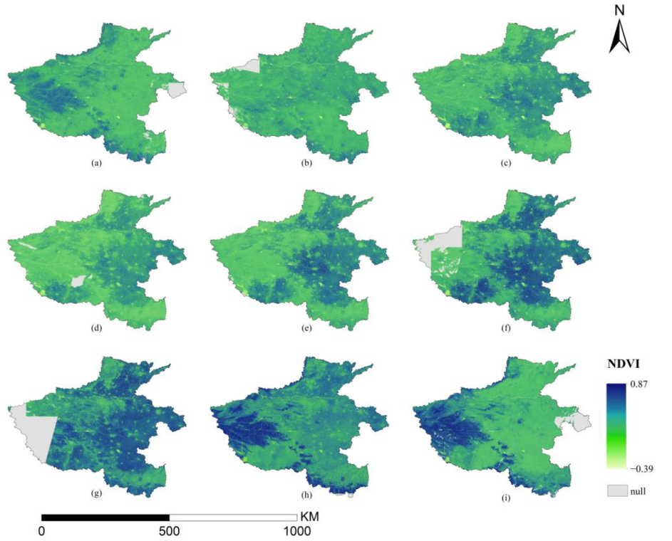
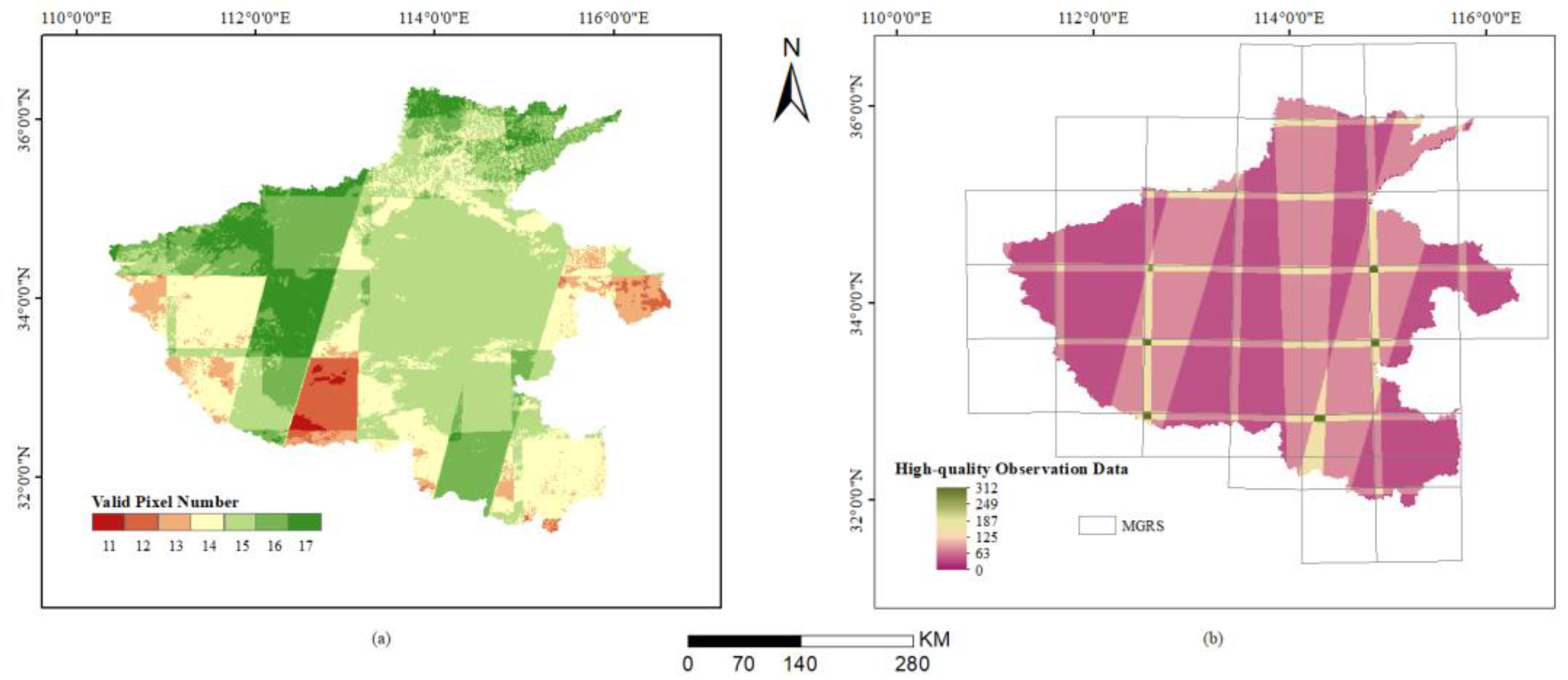
The time-series NDVI data and the distribution map of the total number of valid observations and valid images were obtained (Figure 4 and Figure 5).
There are invalid values of NDVI in some periods in the study area, such as the yellow area in Figure 4, and there is a large difference in the number of effective pixel observations in the entire growth period of winter wheat, such as those in Figure 5a. Therefore, when using the TWDTW method, the standard time-series curve is difficult to match.
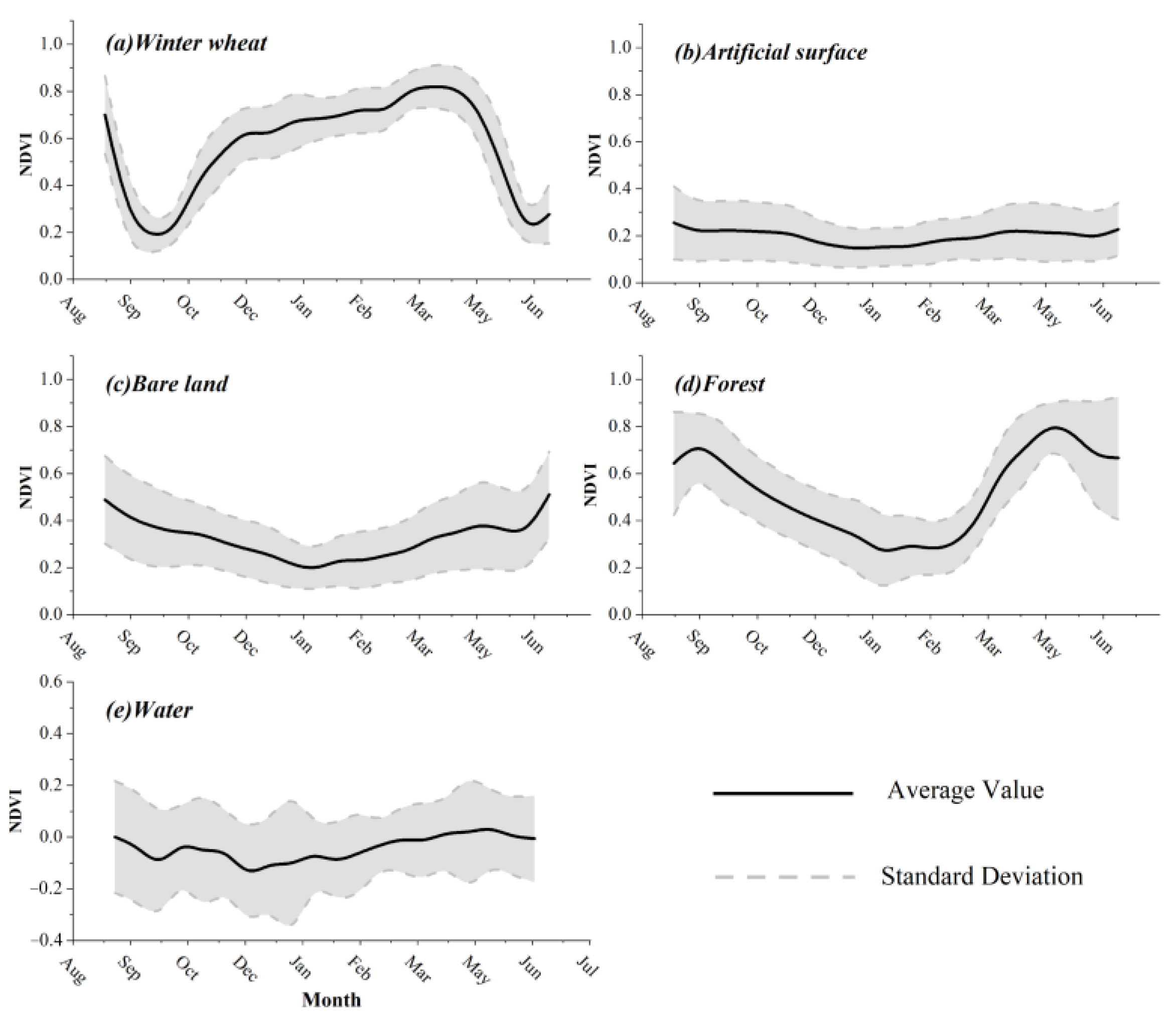
Using the training data to sample the time-series images, the standard change curves of different ground features were obtained, as shown in Figure 6.
There were obvious differences in the NDVI changes between the winter wheat and other ground features, providing intuitive raw data for the E-TWDTW method to extract winter wheat. In October, the winter wheat had just been planted, and the NDVI was still very low, close to the land level. With time, the growth of wheat leaves caused the NDVI value to gradually increase, which shows the opposite trend to other ground cover types and has a higher value compared to the other ground feature types. Until the milk maturity phase in the following year, the NDVI began to decrease significantly due to the influence of the content of chlorophyll in leaves. Finally, the NDVI returned to a low value close to the bare land when the wheat had been harvested at its maturity phase. The water body was kept at a very low position, close to zero. The values of the artificial surface and the bare land were close and fluctuated in the fixed range from 0.2 to 0.5. The value of forest first decreased and then increased over time, crossing the NDVI curve of wheat in November and April.

3.2. E-TWDTW Dissimilarity and Winter Wheat Map

The E-TWDTW dissimilarity indicates the variation between the time-series curve at a specific pixel and the standard change curve of a special feature type, which has a negative correlation with the possibility that a pixel belongs to the feature type. After applying the proposed E-TWDTW curve match algorithm to the NDVI time-series data, the dissimilarity maps between multiple standard change curves were obtained, shown in Figure 7.
Furthermore, after a dissimilarity magnitude comparison, the thematic map of winter wheat of Henan Province was obtained. The winter wheat planting areas were mainly distributed in the plains and concentrated in the central and eastern regions of the province, as shown in Figure 8, which is the same as that of the E-TWDTW dissimilarity value of winter wheat in Figure 7—low in the east and middle, and high in the northwest and south. The statistics based on DEM data showed that 78.12% of wheat was distributed in areas with an altitude of below 100 m, 17.42% was distributed in areas with an altitude in the range of 100–200 m, and 1% was in areas with an altitude of above 500 m. The distribution is consistent with human understanding and objective truth that the plains are more suitable for wheat sowing and harvesting.

3.3. Accuracy Assessment

The results of using validation sample points to evaluate the accuracy of the mapping product are shown in Table 3. The overall accuracy and the Kappa coefficient were 97.98% and 0.9469, respectively, verifying the reliability of the E-TWDTW method at the level of quantitative evaluation.
The comparison results with the 2019 China Statistical Yearbook data are shown in Table 4. At the provincial scale, there is a certain underestimation in the extraction results of the E-TWDTW method, but the agricultural consistency is 98.54%, which verifies that the E-TWDTW method is at the level of statistical evaluation reliability.
Furthermore, a microscopic comparison of the E-TWDTW and RF mapping results of the typical landforms in different subregions was performed to compare the spatial details of the obtained extraction results. In areas where winter wheat was planted and concentrated (Figure 9a–c), the mapping effects obtained by the two classification algorithms were similar, but under the mountain terrain, the extraction result of the E-TWDTW algorithm was better than that of the RF classifier. It can be seen that the result of the RF missed much wheat information, as shown in Figure 9d. Considering phenological differences of different spatial extents, the reason could be that the training features extracted by the RF classifier were difficult to suit the whole study area. The E-TWDTW algorithm could dynamically adjust different nodes so that the impact was avoided.

4. Discussion

4.1. A Sensitivity to Training Data Amount

In order to test the sensitivity of the E-TWDTW method to the training sample size, multiple sets of comparative experiments were conducted. In the experiments, the training set size was 100%, 50%, 25%, and 20% of the original training set size. In order to reduce the error caused by random sampling, we consider the adaptability of the E-TWDTW method by integrating the results of multiple extractions. The accuracy of the results obtained using different data sizes is shown in Table 5.
Under the same validation sample sets, overall, the TWDTW and E-TWDTW methods achieved higher accuracy than RF. The user accuracy obtained by the three methods was relatively stable, but the producer accuracy and Kappa coefficient of the result of the RF classifier gradually decreased with the number of training samples, eventually reaching 59.34% and 0.6788, respectively. Unlike the RF classifier, the E-TWDTW and TWDTW method did not show a significant decrease and maintained a high value of producer accuracy and Kappa coefficient for all data sizes.
Although there is no obvious advantage in the accuracy of the extraction results between the E-TWDTW method and TWDTW under different training data sets due to the complement of missing pixels, while the TWDTW method requires image synthesis at an interval of 30d to reduce the invalid value, the E-TWDTW method uses 15d as the synthesis interval to reduce the amount of data usage. Therefore, the E-TWDTW method can use more time to extract winter wheat, thereby reducing remote-sensing data usage. Considering that the collection of training data consumes much manpower and material resources, the E-TWDTW method represents a promising solution for identifying winter wheat or other crops, especially in regions with few ground labels.

4.2. Early Extraction Ability of E-TWDTW

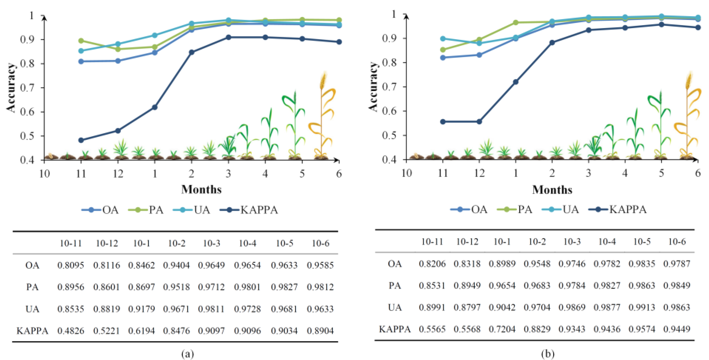
Obtaining accurate planting information before crop harvesting is practical and valuable for agricultural production [48]. To evaluate the ability of the proposed E-TWDTW method for the early season mapping of winter wheat, a series of comparative experiments were conducted by changing the size of the span of the time-series data. The results of the accuracy assessment are shown in Figure 10.
As the time span expanded, various indicators of the accuracy assessment of TWDTW and the E-TWDTW method showed a similar upward trend. From October to December, when the number of images increased, the indicator values increased significantly. Then, from December to February of the following year, the increase rate reduced at first and then gradually increased. Lastly, from March to June, all indicators remained relatively stable without large changes.
Specifically, the indicators’ values showed significant increments from January to March. For the E-TWDTW method, the Kappa coefficient increased from 0.7204 to 0.9343, and the UA increased from 89.91% to 98.69%. After that period, all indicators maintained relatively high values.
From October to December, the low performance of the accuracy evaluation indicators, especially the Kappa, may be due to the fact that the number of valid images in the time range is too small. Therefore, with the expansion of the time span, various accuracy evaluation indicators also gradually increase. From January to March, winter wheat entered the overwintering period, and the accuracy evaluation index showed a significant increase, which was in line with the previous analysis that the NDVI time-series curve of winter wheat was significantly different from the NDVI time-series curve of other land types during the overwintering period. After May, the evaluation index of winter wheat extraction accuracy showed a slight downward trend because, at this time, winter wheat in some areas of Henan Province entered the mature stage, and the NDVI of winter wheat planting areas after harvesting was similar to that of bare land, which made it easy to cause misclassification.
At the same time, from the perspective of the whole winter wheat growth period, the E-TWDTW method showed higher accuracy in different time spans compared with TWDTW, especially before the stage of overwintering. The result shows that the E-TWDTW method could achieve accurate planting information extraction of winter wheat almost three months before the harvesting season.

4.3. Temporal Suitability

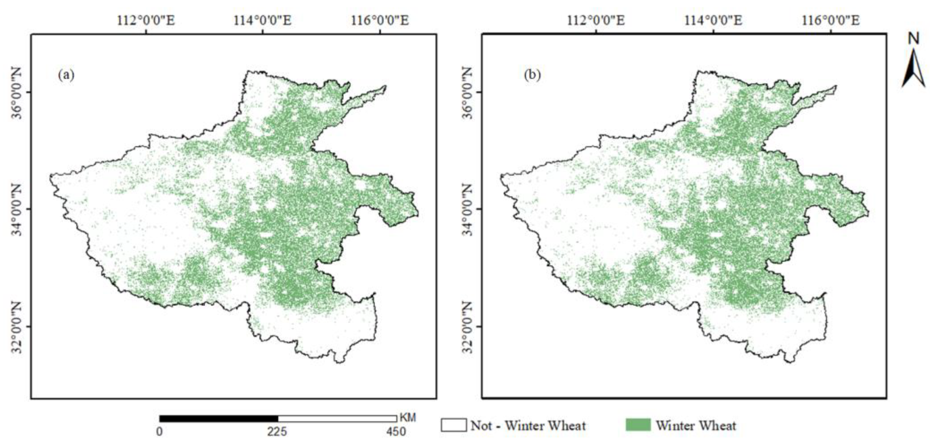
Based on the existing 2019 winter wheat sample points in Henan Province, the 2018 and 2020 winter wheat planting areas in Henan Province were extracted to verify the time suitability of the E-TWDTW method and the calculated NDVI standard time-series curve. The accuracy evaluation and extraction results are shown in Table 6 and Figure 11.
The planting area and spatial distribution of winter wheat in Henan Province in 2018 and 2020 did not change significantly compared with 2019. The overall spatial distribution was in the central and eastern plains of Henan Province, which was in line with the change in the law of the cultivated land area in a short period of time and China’s policy of ensuring cultivated land area in recent years.
When the selected 2019 sample and the prepared NDVI time-series standard curve were applied to the extraction of winter wheat in other years, the accuracy evaluation index of the extraction results decreased compared with 2019, but the overall accuracy, producer accuracy, and user accuracy were all above 96%. Both the Kappa coefficient and the agricultural consistency evaluation remain above 0.9. Therefore, the E-TWDTW method is considered to have better time suitability.
From 2018 to 2020, the planting area of winter wheat in Henan Province showed a slow reduction trend, and the extraction accuracy evaluation results in 2020 were slightly worse than those in 2019. The reason is that there may be changes in 2020 in the land use types of the sample points from 2019, resulting in inconsistent classification results.

5. Conclusions

In this study, we proposed a phenology-based algorithm named E-TWDTW based on the TWDTW algorithm and GEE platform and used the Sentinel-2 data to extract the acreage of winter wheat in Henan Province. The mapping product had a reliable evaluation result, with Overall Accuracy and the Kappa Coefficient being 97.98% and 0.9469, respectively.
The comparative experiment results show:
  • Compared with the prototype TWDTW method, the E-TWDTW method reduces the usage of remote-sensing data while maintaining extraction accuracy, thereby improving extraction efficiency.
  • The E-TWDTW method shows its sensitivity with a small training sample close to the TWDTW method with fewer images, which is better than RF. In the case of large-scale training samples, the extraction results of E-TWDTW and the Random Forest are similar, but when the number of training samples gradually decreases, the extraction advantages of the E-TWDTW algorithm gradually become obvious. This phenomenon indicates that the E-TWDTW algorithm has greater potential for crop identification research in areas where it is difficult to obtain samples.
  • In addition, in the experiment of early recognition ability, the extraction performance of the E-TWDTW algorithm can reach a high level three months before the winter wheat harvest, which shows that the E-TWDTW algorithm has a very good practical prospect so that we can prepare for further production forecasts and harvesting of winter wheat.
  • Compared with the TWDTW method, although the E-TWDTW method reduces the use of data, it still needs to improve the accuracy and the consistency of the extraction results. In future research, it is proposed to further improve the result’s accuracy of the E-TWDTW method by combining multiple vegetation indexes and different growth periods data.

Author Contributions

Conceptualization, X.W.; methodology, X.W.; software, M.H. and C.Y.; validation, S.S. and Z.H.; formal analysis, M.H.; data curation, Z.H.; writing—original draft preparation, M.H. and C.Y.; writing—review and editing, S.S. and Z.H.; project administration, X.W. and L.X. All authors have read and agreed to the published version of the manuscript.

Funding

This research was funded by the key scientific and technological project of Henan Province, grant number 212102210137, the Natural Science Foundation of Henan, grant number 212300410292, the key research project of Higher Education of Henan Province, China, grant number 21A420006, and the Open Fund of National Engineering Research Center for Geographic Information System, China University of Geosciences, Wuhan 430074, China, grant number 2021KFJJ04.

Data Availability Statement

Not applicable.

Conflicts of Interest

The authors declare no conflict of interest.

References

  1. Mkhabela, M.S.; Bullock, P.; Raj, S.; Wang, S.; Yang, Y. Crop yield forecasting on the Canadian Prairies using MODIS NDVI data. Agric. For. Meteorol. 2011, 151, 385–393. [Google Scholar] [CrossRef]
  2. Shiferaw, B.; Smale, M.; Braun, H.; Duveiller, E.; Reynolds, M.; Muricho, G. Crops that feed the world 10. Past successes and future challenges to the role played by wheat in global food security. Food Secur. 2013, 5, 291–317. [Google Scholar] [CrossRef] [Green Version]
  3. Qiu, B.; Luo, Y.; Tang, Z.; Chen, C.; Lu, D.; Huang, H.; Chen, Y.; Chen, N.; Xu, W. Winter wheat mapping combining variations before and after estimated heading dates. ISPRS J. Photogramm. 2017, 123, 35–46. [Google Scholar] [CrossRef]
  4. Yang, Y.; Tao, B.; Ren, W.; Zourarakis, D.P.; Masri, B.E.; Sun, Z.; Tian, Q. An Improved Approach Considering Intraclass Variability for Mapping Winter Wheat Using Multitemporal MODIS EVI Images. Remote Sens. 2019, 11, 1191. [Google Scholar] [CrossRef] [Green Version]
  5. Zhang, M.; Lin, H. Object-based rice mapping using time-series and phenological data. Adv. Space Res. 2019, 63, 190–202. [Google Scholar] [CrossRef]
  6. Pan, Y.; Li, L.; Zhang, J.; Liang, S.; Zhu, X.; Sulla-Menashe, D. Winter wheat area estimation from MODIS-EVI time series data using the Crop Proportion Phenology Index. Remote Sens. Environ. 2012, 119, 232–242. [Google Scholar] [CrossRef]
  7. Huang, J.; Tian, L.; Liang, S.; Ma, H.; Becker-Reshef, I.; Huang, Y.; Su, W.; Zhang, X.; Zhu, D.; Wu, W. Improving winter wheat yield estimation by assimilation of the leaf area index from Landsat TM and MODIS data into the WOFOST model. Agr. For. Meteorol. 2015, 204, 106–121. [Google Scholar] [CrossRef] [Green Version]
  8. Chen, Z.X.; Ren, J.Q.; Tang, H.J.; Shi, Y.; Leng, P.; Liu, J.; Wang, L.M.; Wu, W.B.; Yao, Y.M.; Hasiyuya. Progress and perspectives on agricultural remote sensing research and applications in China. J. Remote Sens. 2016, 20, 748–767. [Google Scholar]
  9. Gallego, F.J.; Kussul, N.; Skakun, S.; Kravchenko, O.; Shelestov, A.; Kussul, O. Efficiency assessment of using satellite data for crop area estimation in Ukraine. Int. J. Appl. Earth Obs. 2014, 29, 22–30. [Google Scholar] [CrossRef]
  10. Wardlow, B.D.; Egbert, S.L.; Kastens, J.H. Analysis of time-series MODIS 250 m vegetation index data for crop classification in the US Central Great Plains. Remote Sens. Environ. 2007, 108, 290–310. [Google Scholar] [CrossRef] [Green Version]
  11. Skakun, S.; Franch, B.; Vermote, E.; Roger, J.; Becker-Reshef, I.; Justice, C.; Kussul, N. Early season large-area winter crop mapping using MODIS NDVI data, growing degree days information and a Gaussian mixture model. Remote Sens. Environ. 2017, 195, 244–258. [Google Scholar] [CrossRef]
  12. Jain, M.; Mondal, P.; DeFries, R.S.; Small, C.; Galford, G.L. Mapping cropping intensity of smallholder farms: A comparison of methods using multiple sensors. Remote Sens. Environ. 2013, 134, 210–223. [Google Scholar] [CrossRef] [Green Version]
  13. Wei, M.; Qiao, B.; Zhao, J.; Zuo, X. The area extraction of winter wheat in mixed planting area based on Sentinel-2 a remote sensing satellite images. Int. J. Parallel Emergent Distrib. Syst. 2020, 35, 297–308. [Google Scholar] [CrossRef]
  14. Belgiu, M.; Csillik, O. Sentinel-2 cropland mapping using pixel-based and object-based time-weighted dynamic time warping analysis. Remote Sens. Environ. 2018, 204, 509–523. [Google Scholar] [CrossRef]
  15. Carmelo, R.F.; Giuseppe, M.; Maurizio, P. Land Cover classification and change-detection analysis using multi-temporal remote sensed imagery and landscape metrics. Eur. J. Remote Sens. 2012, 45, 1–18. [Google Scholar]
  16. Kyere, I.; Astor, T.; Graß, R.; Wachendorf, M. Multi-Temporal Agricultural Land-Cover Mapping Using Single-Year and Multi-Year Models Based on Landsat Imagery and IACS Data. Agronomy 2019, 9, 309. [Google Scholar] [CrossRef] [Green Version]
  17. Tian, H.; Huang, N.; Niu, Z.; Qin, Y.; Pei, J.; Wang, J. Mapping Winter Crops in China with Multi-Source Satellite Imagery and Phenology-Based Algorithm. Remote Sens. 2019, 11, 820. [Google Scholar] [CrossRef] [Green Version]
  18. Jin, Z.; Azzari, G.; You, C.; Di Tommaso, S.; Aston, S.; Burke, M.; Lobell, D.B. Smallholder maize area and yield mapping at national scales with Google Earth Engine. Remote Sens. Environ. 2019, 228, 115–128. [Google Scholar] [CrossRef]
  19. Sun, H.; Xu, A.; Lin, H.; Zhang, L.; Mei, Y. Winter wheat mapping using temporal signatures of MODIS vegetation index data. Int. J. Remote Sens. 2012, 33, 5026–5042. [Google Scholar] [CrossRef]
  20. Zhang, Z.; Hua, L.; Wei, Q.; Li, J.; Wang, J. Recognition and Changes Analysis of Complex Planting Patterns Based Time Series Landsat and Sentinel-2 Images in Jianghan Plain, China. Agronomy 2022, 12, 1773. [Google Scholar] [CrossRef]
  21. Tang, J.; Zhang, X.; Chen, Z.; Bai, Y. Crop Identification and Analysis in Typical Cultivated Areas of Inner Mongolia with Single-Phase Sentinel-2 Images. Sustainability 2022, 14, 12789. [Google Scholar] [CrossRef]
  22. Jordan, M.I.; Mitchell, T.M. Machine learning: Trends, perspectives, and prospects. Science 2015, 349, 255–260. [Google Scholar] [CrossRef] [PubMed]
  23. Yang, Z.; Zhang, H.; Lyu, X.; Du, W. Improving Typical Urban Land-Use Classification with Active-Passive Remote Sensing and Multi-Attention Modules Hybrid Network: A Case Study of Qibin District, Henan, China. Sustainability 2022, 14, 14723. [Google Scholar] [CrossRef]
  24. Atzberger, C. Advances in Remote Sensing of Agriculture: Context Description, Existing Operational Monitoring Systems and Major Information Needs. Remote Sens. 2013, 5, 949–981. [Google Scholar] [CrossRef] [Green Version]
  25. Liakos, K.G.; Busato, P.; Moshou, D.; Pearson, S.; Bochtis, D. Machine learning in agriculture: A review. Sensors 2018, 18, 2674. [Google Scholar] [CrossRef] [Green Version]
  26. Millard, K.; Richardson, M. On the importance of training data sample selection in random forest image classification: A case study in peatland ecosystem mapping. Remote Sens. 2015, 7, 8489–8515. [Google Scholar] [CrossRef] [Green Version]
  27. Maus, V.; Camara, G.; Cartaxo, R.; Sanchez, A.; Ramos, F.M.; de Queiroz, G.R. A Time-Weighted Dynamic Time Warping Method for Land-Use and Land-Cover Mapping. IEEE J. Sel. Top. Appl. Earth Obs. Remote Sens. 2016, 9, 3729–3739. [Google Scholar] [CrossRef]
  28. Dong, J.; Fu, Y.; Wang, J.; Tian, H.; Fu, S.; Niu, Z.; Han, W.; Zheng, Y.; Huang, J.; Yuan, W. Early-season mapping of winter wheat in China based on Landsat and Sentinel images. Earth Syst. Sci. Data 2020, 12, 3081–3095. [Google Scholar] [CrossRef]
  29. Deines, J.M.; Kendall, A.D.; Crowley, M.A.; Rapp, J.; Cardille, J.A.; Hyndman, D.W. Mapping three decades of annual irrigation across the US High Plains Aquifer using Landsat and Google Earth Engine. Remote Sens. Environ. 2019, 233, 111400. [Google Scholar] [CrossRef]
  30. Dong, J.; Xiao, X.; Menarguez, M.A.; Zhang, G.; Qin, Y.; Thau, D.; Biradar, C.; Moore, B. Mapping paddy rice planting area in northeastern Asia with Landsat 8 images, phenology-based algorithm and Google Earth Engine. Remote Sens. Environ. 2016, 185, 142–154. [Google Scholar] [CrossRef] [Green Version]
  31. Huang, H.; Chen, Y.; Clinton, N.; Wang, J.; Wang, X.; Liu, C.; Gong, P.; Yang, J.; Bai, Y.; Zheng, Y.; et al. Mapping major land cover dynamics in Beijing using all Landsat images in Google Earth Engine. Remote Sens. Environ. 2017, 202, 166–176. [Google Scholar] [CrossRef]
  32. National Bureau of Statistics People’s Republic of China. China Statistical Yearbook; China Statistics Press: Beijing, China, 2020; p. 375. [Google Scholar]
  33. Sheng, L.; He, Y.J.; Wu, Q.; Wang, F. Comparative study on accuracy of winter wheat production by remote sensing monitoring in Henan province. China Agric. Inf. 2018, 30, 95–102. (In Chinese) [Google Scholar]
  34. Yang, G.; Yu, W.; Yao, X.; Zheng, H.; Cao, Q.; Zhu, Y.; Cao, W.; Cheng, T. AGTOC: A novel approach to winter wheat mapping by automatic generation of training samples and one-class classification on Google Earth Engine. Int. J. Appl. Earth Obs. Geo-Inf. 2021, 102, 102446. [Google Scholar] [CrossRef]
  35. Gorelick, N.; Hancher, M.; Dixon, M.; Ilyushchenko, S.; Thau, D.; Moore, R. Google Earth Engine: Planetary-scale geospatial analysis for everyone. Remote Sens. Environ. 2017, 202, 18–27. [Google Scholar] [CrossRef]
  36. Immitzer, M.; Vuolo, F.; Atzberger, C. First experience with Sentinel-2 data for crop and tree species classifications in central Europe. Remote Sens. 2016, 8, 166. [Google Scholar] [CrossRef]
  37. Zhou, Z.; Ding, Y.; Shi, H.; Cai, H.; Fu, Q.; Liu, S.; Li, T. Analysis and prediction of vegetation dynamic changes in China: Past, present and future. Ecol. Indic. 2020, 117, 106642. [Google Scholar] [CrossRef]
  38. Muda, L.; Begam, M.; Elamvazuthi, I. Voice recognition algorithms using mel frequency cepstral coefficient (MFCC) and dynamic time warping (DTW) techniques. arXiv 2010, arXiv:1003.4083. [Google Scholar]
  39. Shanker, A.P.; Rajagopalan, A.N. Off-line signature verification using DTW. Pattern Recogn. Lett. 2007, 28, 1407–1414. [Google Scholar] [CrossRef]
  40. Guan, X.; Huang, C.; Liu, G.; Meng, X.; Liu, Q. Mapping rice cropping systems in Vietnam using an NDVI-based time-series similarity measurement based on DTW distance. Remote Sens. 2016, 8, 19. [Google Scholar] [CrossRef] [Green Version]
  41. Qiu, P.; Wang, X.; Cha, M.; Li, Y. Crop Identification Based on TWDTW Method and Time Series GF-1 WFV. Sci. Acricultura Sin. 2019, 52, 2951–2961. [Google Scholar] [CrossRef]
  42. Zheng, Y.; dos Santos Luciano, A.C.; Dong, J.; Yuan, W. High-resolution map of sugarcane cultivation in Brazil using a phenology-based method. Earth Syst. Sci. Data 2022, 14, 2065–2080. [Google Scholar] [CrossRef]
  43. Pal, M. Random forest classifier for remote sensing classification. Int. J. Remote Sens. 2005, 26, 217–222. [Google Scholar] [CrossRef]
  44. Belgiu, M.; Drăguţ, L. Random forest in remote sensing: A review of applications and future directions. ISPRS J. Photogramm. 2016, 114, 24–31. [Google Scholar] [CrossRef]
  45. Congalton, R.G.; Green, K. Assessing the Accuracy of Remotely Sensed Data: Principles and Practices; CRC Press: Boca Raton, FL, USA, 2019. [Google Scholar]
  46. Congalton, R.G. A review of assessing the accuracy of classifications of remotely sensed data. Remote Sens. Environ. 1991, 37, 35–46. [Google Scholar] [CrossRef]
  47. Cohen, J. A Coefficient of Agreement for Nominal Scales. Educ. Psychol. Meas. 1960, 20, 37–46. [Google Scholar] [CrossRef]
  48. Torres-Sánchez, J.; Pena, J.M.; de Castro, A.I.; López-Granados, F. Multi-temporal mapping of the vegetation fraction in early-season wheat fields using images from UAV. Comput. Electron. Agr. 2014, 103, 104–113. [Google Scholar] [CrossRef]
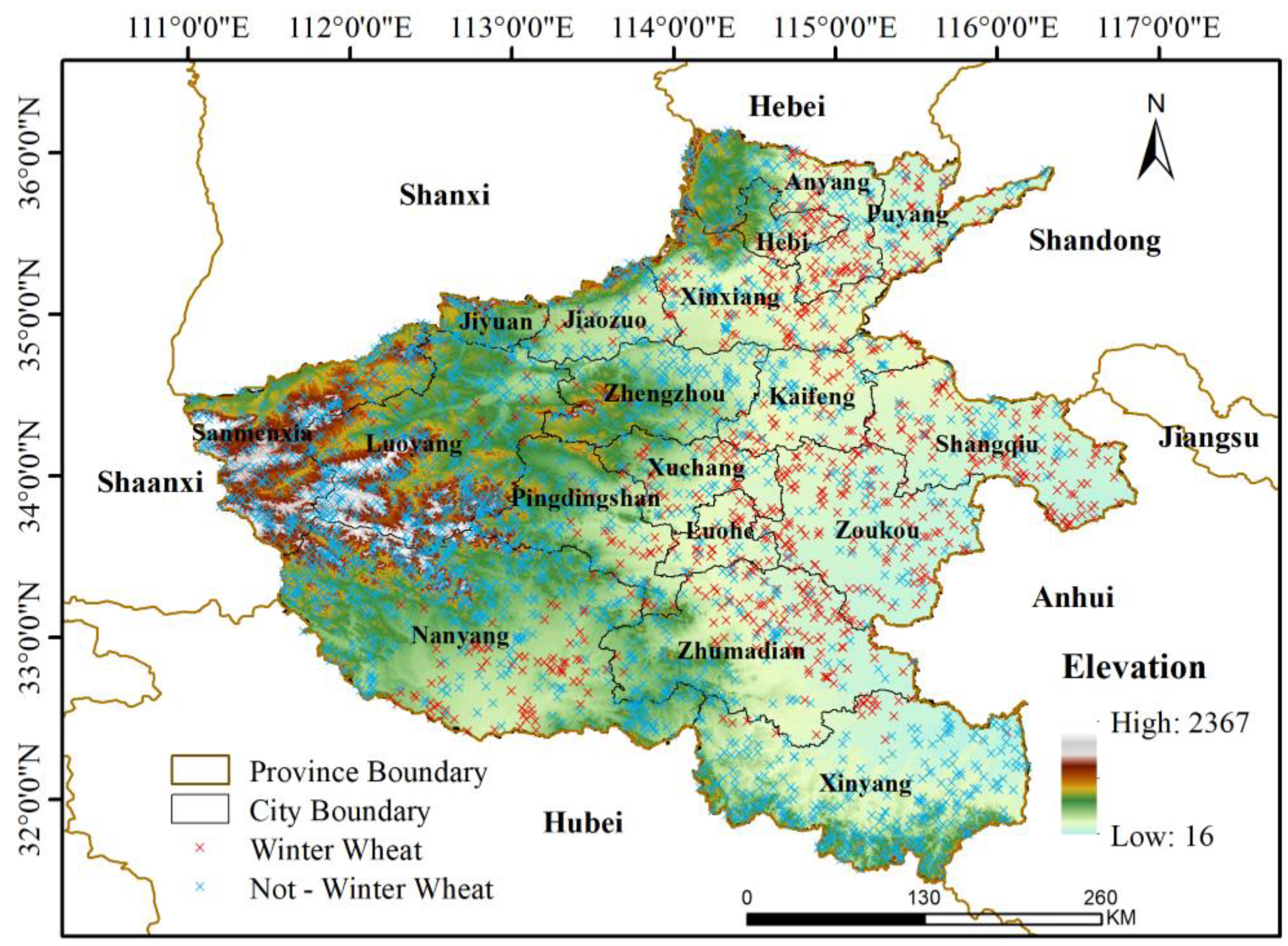
Figure 1. Location of Henan Province and the altitude distribution.
Sustainability 15 01490 g001
Figure 2. Overall flow chart of this study.
Sustainability 15 01490 g002
Figure 3. Schematic diagram of the E-TWDTW method. (a) The original NDVI image in January 2020; (b) processing original curve by adjustment and interpolation of invalid values; (c) the processed complete NDVI image in January 2020.
Sustainability 15 01490 g003
Figure 4. The NDVI images of different time ranges covering the winter wheat growth period from 2019 to 2020. (a) October 2019; (b) November 2019; (c) December 2019; (d) January 2020; (e) February 2020; (f) March 2020; (g) April 2020; (h) May 2020; (i) June 2020.
Sustainability 15 01490 g004
Figure 5. Distribution map of the total number of valid values and images in the period from October 1, 2019, to June 30, 2020. The valid pixel value refers to the mean value of pixel values in the processed image collection. (a) Valid values, (b) High-quality observation data.
Sustainability 15 01490 g005
Figure 6. NDVI change curves of different ground feature types. The water body was kept at a very low position, close to zero. The values of the artificial surface and the bare land were close and fluctuated in the fixed range from 0.2 to 0.5. The value of forest first decreased and then increased over time, crossing the NDVI curve of wheat in November and April.
Sustainability 15 01490 g006
Figure 7. The E-TWDTW dissimilarity maps between (a) winter wheat, (b) artificial surface, (c) bare land, (d) forest, (e) water standard change curves. The color change from yellow to blue represents the transition of dissimilarity from a low value to a high value.
Sustainability 15 01490 g007
Figure 8. Winter wheat planting area extraction results. Five sub-regions denoted as a, b, c, d, and e were used as representative physiognomies for the microscopic perspective of two extraction methods, which are shown in Figure 9.
Sustainability 15 01490 g008
Figure 9. Five subsets of the winter wheat map; from top to bottom—the true color (RGB), E-TWDTW, and RF mapping results. The spatial characteristics: (a) close to the highway and (b) village, (c) concentrated plots of farmland, (d) highland, and (e) riverside.
Sustainability 15 01490 g009
Figure 10. Early recognition ability of winter wheat. (a) TWDTW method, (b) the E-TWDTW method.
Sustainability 15 01490 g010
Figure 11. Winter wheat planting area extraction results in 2018 and 2020. (a) 2018, (b) 2020.
Sustainability 15 01490 g011
Table 1. Image usage.
Time PeriodImage Usage
2018.10.1–2019.6.13014
2019.10.1–2020.6.13038
2020.10.1–2021.6.13007
Table 2. Numbers of training and validation samples.
Land Cover ClassTraining PixelsValidation Pixels
Winter wheat309482
Artificial surface215324
Water5173
Bare land228307
Forest452687
Table 3. Confusion matrix obtained by independent validation samples.
ClassificationValidation SamplesTotalUA
WheatNot-Wheat
Wheat181223183598.74%
Not-wheat27608635
Total18396352470
PA98.53% OA = 97.98%Kappa = 0.9469
Table 4. Comparison of extraction area and statistical area of winter wheat.
Extraction Area/km2Statistical Area /km2High(+)/under(−)EstimateAgricultural Consistency
E-TWDTW56231.957066.5−834.698.54%
TWDTW55447.3−1619.297.16%
RF53768.7−3297.894.22%
Table 5. Accuracy assessment results for different training data sizes.
E-TWDTWRFTWDTW
Training Sample RatioOA
(%)
PA
(%)
UA
(%)
KappaOA
(%)
PA
(%)
UA
(%)
KappaOA
(%)
PA
(%)
UA
(%)
KAPPA
100%97.8798.4998.630.944994.5580.2998.220.848597.1898.4997.710.9263
50%98.3398.6799.130.957492.7973.4498.060.794698.0598.7798.590.9493
25%98.0698.5598.920.912790.0762.6698.050.705597.8098.5598.500.9420
20%97.8998.5398.750.946889.3259.3498.620.678898.1098.5998.850.9501
Table 6. Accuracy assessment results for winter wheat extraction area in 2018 to 2020.
OA
(%)
PA
(%)
UA
(%)
KappaExtraction Area (/km2)Statistical Area (/km2)Agricultural Consistency (%)
201897.2398.4297.850.927853998.2.5739991.63
201997.9898.5398.740.946956231.95706798.54
202097.0797.7098.330.924557986.75673797.84
Disclaimer/Publisher’s Note: The statements, opinions and data contained in all publications are solely those of the individual author(s) and contributor(s) and not of MDPI and/or the editor(s). MDPI and/or the editor(s) disclaim responsibility for any injury to people or property resulting from any ideas, methods, instructions or products referred to in the content.