Change Characteristics of Soil Organic Carbon and Soil Available Nutrients and Their Relationship in the Subalpine Shrub Zone of Qilian Mountains in China

Abstract

Studying the spatial and temporal distribution of soil organic carbon (SOC) content in high-altitude mountainous areas and its correlation with soil nutrients provides a basis for understanding soil carbon stocks and the factors affecting the local carbon cycle. Based on soil samples collected from a semi-sunny slope and semi-shady slope in the subalpine shrub zone of the eastern Qilian Mountains from May to October 2019, we studied the temporal and spatial changes in SOC and soil available nutrients and their relationships. The results showed that SOC content and soil nutrients were greater on the semi-shady slope than on the semi-sunny slope during the growing season and decreased with an increase in soil depth in different slope directions, showing obvious surface aggregation. The soil available nitrogen (SAN) content was consistent with the SOC content and exhibited greater synchronization. SOC was significantly positively correlated with soil available nutrients in the study area during the whole growing season. However, the correlation between SOC and soil nutrients varied among the different soil layers and slope orientations. The SOC content was more obviously correlated with the SAN content in the soil layer at a depth of 30–40 cm (r = 0.67, p < 0.05) on the semi-shady slope. The SOC content was more obviously correlated with soil-available phosphorus (SAP) content in the soil layer at a depth of 30–40 cm (r = 0.57) on the semi-sunny slop. The SOC content was more obviously correlated with the SAP content in the soil layer at a depth of 60–70 cm (r = 0.55) and with the soil-available potassium (SAK) content in the soil layer at a depth of 70–80 cm (r = 0.84) on the semi-sunny slope.

1. Introduction

SOC and soil nutrients play pivotal roles in the carbon cycle. SOC, as a crucial element of soil organic matter (SOM), plays a vital role in evaluating soil quality and structure. Meanwhile, soil nutrients, as the cornerstone of soil fertility, have a significant impact on the carbon exchange between plants and the atmosphere, making them highly influential [1]. Given the sensitivity of mountains at high altitudes to environmental factors and their significance as storage sites for SOC [2], studying the spatial and temporal distribution of the SOC content in these regions and its correlation with soil nutrients has become essential for understanding soil carbon stocks and the factors that impact the local carbon cycle.

Various soil factors, such as soil moisture content, soil nutrients, soil texture, climate, and topography, affect the regional SOC content and its dynamic variations [3]. For example, temperature and precipitation affect the SOC content by regulating the decomposition and accumulation of soil organic matter [4]. It is worth noting that the factors impacting the SOC content vary across different soil layers [1]. For instance, the main factor influencing SOC in shallow soil is the climate, while in deep soil, the main factor is clay content, with a significant positive correlation between them [4]. Topography is an important factor influencing the distribution of the SOC content [5]. In mountain ecosystems, topography shapes spatial patterns, and slope direction changes small-scale hydrothermal conditions, leading to different rates of SOC decomposition and accumulation and affecting local SOC content [5,6,7]. Generally, the SOC content is higher on shady slopes than that on sunny slopes [3]. Scholars have extensively researched SOC, especially in high-altitude mountainous areas, regions which are more sensitive to climatic factors [8]. For example, Post et al. [9] showed that the SOC content tended to increase with an increase in altitude and a decrease in temperature. Nie et al. [10] indicated that the warming of the Qinghai–Tibet Plateau increased the potential carbon sink of alpine shrubs. Makarov et al. [11,12] demonstrated that SOC decreased with an increase in soil moisture, and microbial biomass decreased with a decrease in soil moisture. The SOC content was closely related to vegetation cover and depleted as a result of rangeland degradation [2,13]. Tudi et al. [14] studied the western part of Tien Shan and demonstrated a simultaneously elevated relationship between soil organic matter and soil nutrients, but the same relationship was not observed in the east. In addition, human activities have little influence on mountains at high altitude, meaning that they can better reflect the accumulation and depletion of SOC and soil nutrients in their natural state. Therefore, it is important to study the spatial and temporal distribution and influencing factors of SOC in mountains at high altitudes to predict the regional atmosphere–soil feedback mechanism under future climate change scenarios.

Soil available nutrients refers to the nutrients in the soil that can be directly utilized by plants [15]. As the main components of soil available nutrients, the levels of SAN, SAP, and SAK content mainly reflect the ability of the soil to actually supply nitrogen, phosphorus, and potassium to plants [15]. Moreover, the contents of these elements in soils directly affect plant growth and evaluations of soil quality [16,17,18,19]. SOC is closely related to soil available nutrients. Studies have shown that SAN is related to the SOC content in a vertical profile [20] and that the SOC content is mainly related to underground biomass and the SAN content in the soil layer at a depth of 0–40 cm [21]. Changes in soil phosphorus elements were significantly correlated with soil parent materials and organic matter [20]. As with SOC, the SAK content was found to gradually increase in closed grasslands without grazing [22]. A significant positive correlation between SOC and total nitrogen (TN) was found in most land-use types [23]. The SOC content was positively correlated with soil nutrients (available N, P, K) [24].

The Qilian Mountains are an important ecological barrier in the northwest of China. Subalpine shrublands constitute one of the main components of the forest ecosystem in the Qilian Mountains. In recent years, an increasing number of studies have been performed on SOC in the Qilian Mountains [1,24,25,26,27,28]. These studies have primarily analyzed the impacts of soil depth, plant type, climate, soil moisture, soil physicochemical properties, and elevation on the SOC content in the Qilian Mountains [1,26,27,28]. However, few studies have explored the spatial and temporal distribution of SOC and its relationship with soil nutrients in different slope orientations in the subalpine scrubland. Therefore, based on soil samples collected from different slope orientations in the subalpine shrub zone of the eastern Qilian Mountains from May to October 2019, we studied the temporal and spatial changes in SOC and soil available nutrients and their relationships. The aim of this work was to clarify the soil’s carbon sequestration capacity and its influencing factors in the subalpine scrub zone, thereby providing a theoretical basis for the soil carbon cycle in mountains at high altitudes.

2. Data and Research Methods

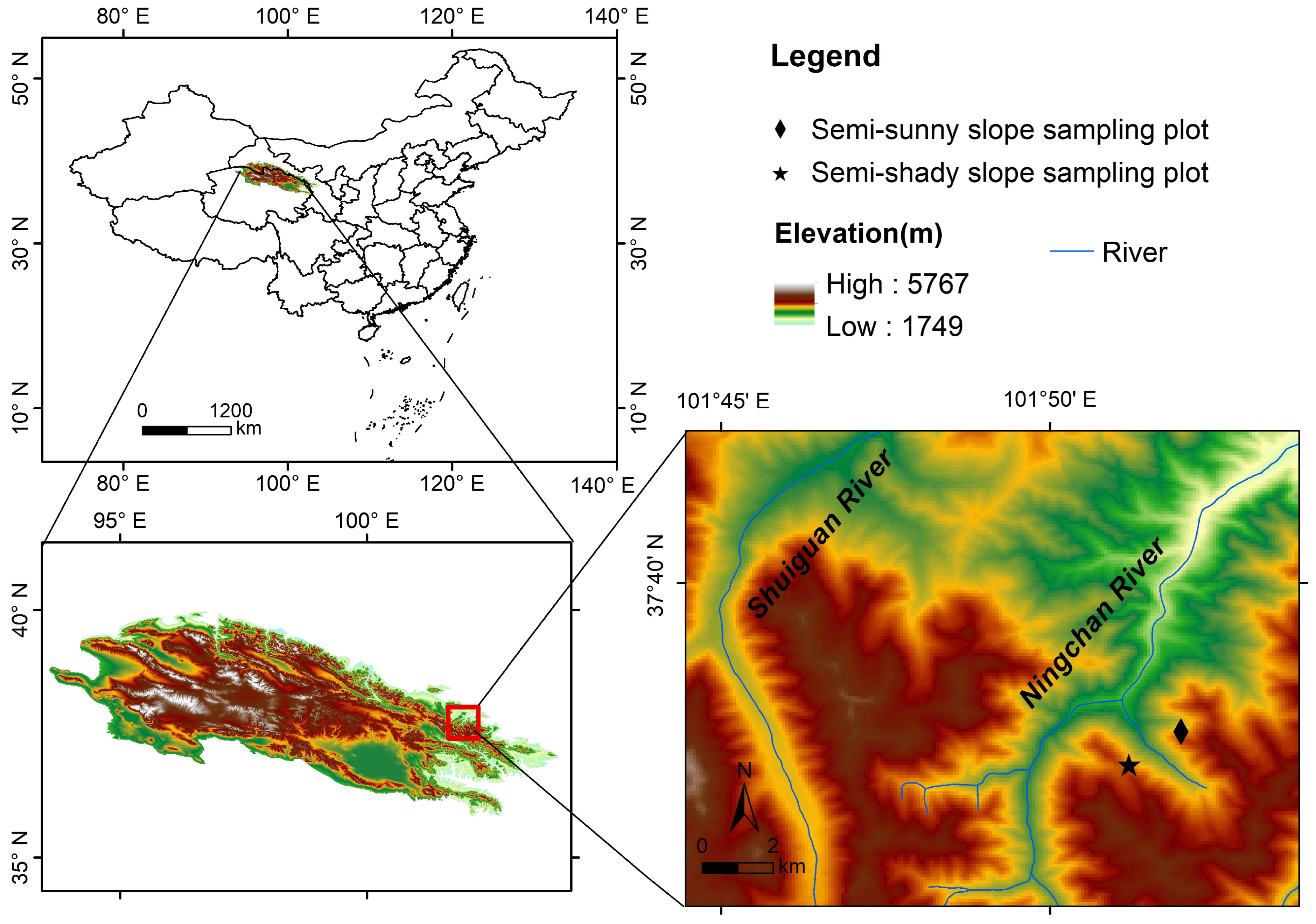
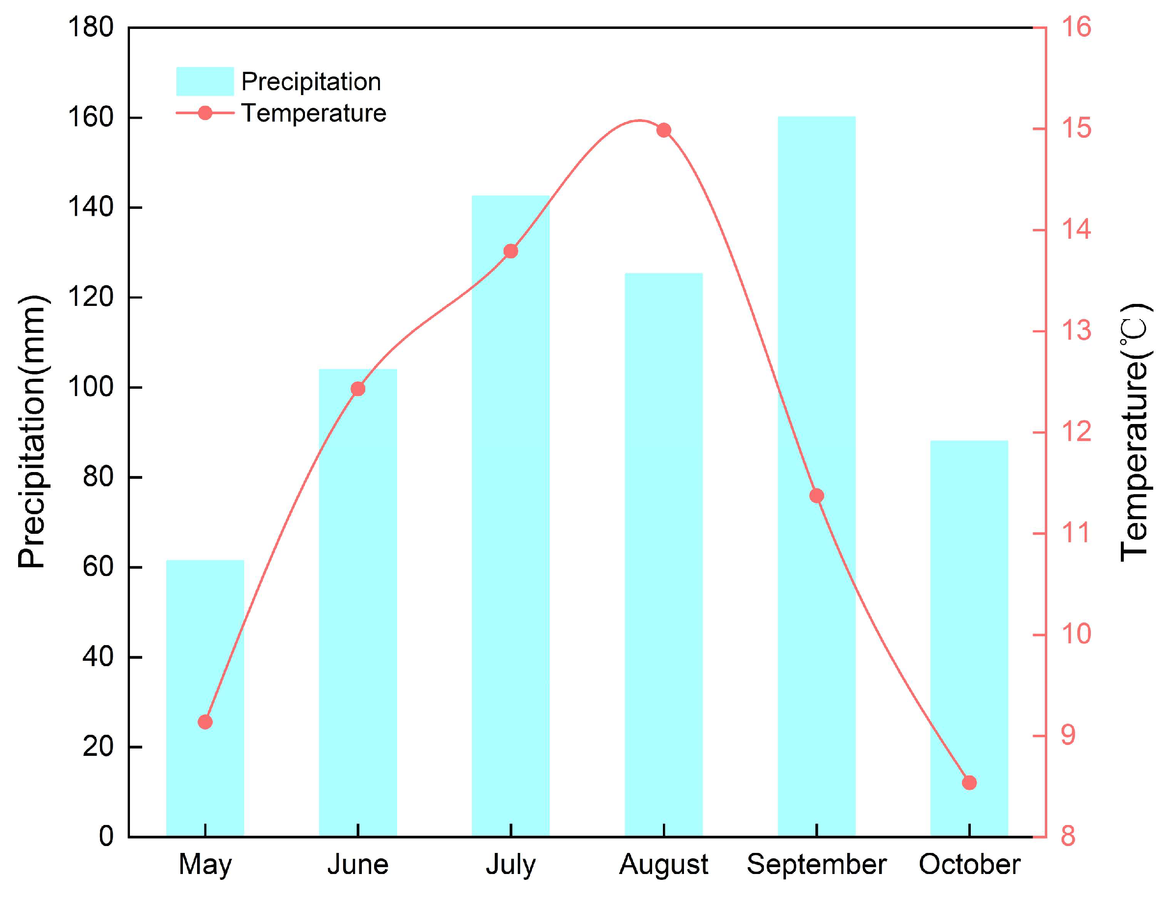
2.1. Description of the Study Area

The study area is located in Shangchigou (37°38′10″ N, 101°41′9″ E, average elevation 3080 m) on the Ningchang River, which is a tributary of the Shiyang River. The area belongs to the subalpine zone on the northern slope of Lenglongling in the eastern Qilian Mountains (Figure 1), which has typical continental and plateau climate characteristics [29]. Lenglongling extends from northwest to southeast [30], with an average annual temperature lower than 6 °C and an annual cumulative precipitation of about 400–600 mm, mainly concentrated in the period from June to September [31] (Figure 2). Due to the influence of complex natural conditions, the soil and vegetation on Qilian Mountain have obvious vertical bands [31]. In the study area, the vegetation distribution is a subalpine shrub–meadow symbiosis, in which the coverage of shrubs can reach over 50%, and the soil type is subalpine shrub meadow soil (Cambisols) with a thickness of about 40–80 cm. The main soil is defined as Cambisols according to the international WRB classification [32]. According to the International Textural Classification, the soils at the sampling plots are loamy in texture (semi-shady slope: clay 8.60%, silt 52.43%, sand 38.75%; semi-sunny slope: clay 9.87%, silt 61.97%, sand 28.16%). The soil-forming matrix in the study area is sandstone [33].

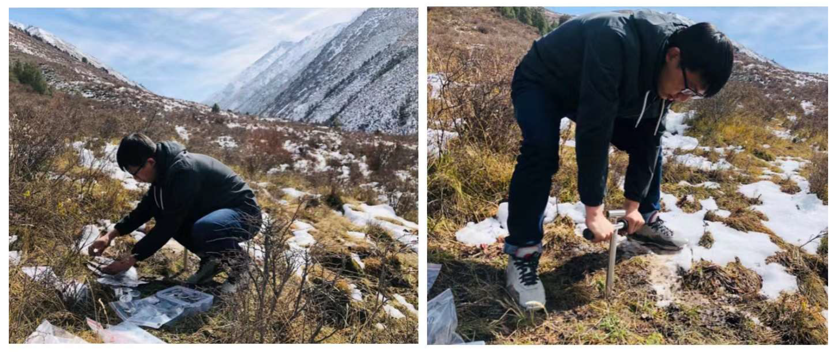
2.2. Sample Collection

Two sample plots on the semi-sunny slope (37°38′10.25″ N, 101°51′13.03″ E, mean elevation 3083 m, 21.01°) and the semi-shady slop (37°38′10.52″ N, 101°51′7.03″ E, mean elevation 3077 m, 32.46°) were established in Shangchigou from May to October 2019 (Figure 1 and Figure 3). In the Qilian Mountain area, Zhu et al. [26] demonstrated that the impact of slope gradient on SOC within the scrub–meadow zone was negligible compared to slope direction. Given that the sampled areas have similar slope values, the effect of the gradient is not considered in this paper. In addition, the study area is affected by light grazing during seasonal pasture conversions, and the impacts of human activities on SOC and soil available nutrients are not considered in this paper.

The distance between the two sample plots was no more than 1 km, and the elevation was no more than 10 m. A sample plot of 2 m × 2 m arranged randomly was established within each sample plot, showing subalpine scrub–meadow symbiosis. Using the adopted diagonal sampling method, samples were collected at intervals of 10 cm. Based on the thickness of the soil layer in the sampling plots, the samples were taken at a depth of 80 cm on the semi-sunny slope and collected from depths of 0–10 cm, 10–20 cm, 20–30 cm, 30–40 cm, 40–50 cm, 50–60 cm, 60–70 cm, and 70–80 cm, respectively. Samples were taken at a depth of 60 cm on the semi-shady slope and were collected from depths of 0–10 cm, 10–20 cm, 20–30 cm, 30–40 cm, 40–50 cm, and 50–60 cm, respectively, which facilitated comparative analyses between multiple layers of soil [25,34]. Each soil sample was mixed with 3 repeated samples, placed into aluminum boxes, and then brought back to the laboratory under a seal. To ensure the accuracy of the data, parallel samples were collected at intervals of less than 10 m in the same plot, using the same method. In total, 560 soil samples were collected (2 slope orientations (semi-sunny and semi-shady slopes) × 2 sample sites (each slope orientation) × 14 soil layers (8 and 6 soil layers for semi-sunny and semi-sunny slopes, respectively) × 10 sampling dates (sampling dates were 21 May, 5 June, 24 June, 6 July, 25 July, 6 August, 18 August, 6 September, 21 September, and 13 October) = 560 samples), of which 280 soil samples were used to determine the soil moisture content, and 280 were used to determine the SOC and soil nutrients.

2.3. Sample Measurement

The SOC content was determined using the potassium dichromate oxidation method [3]. For this process, a soil sample of 0.05 g was weighed and sieved, and 5 mL of potassium dichromate (K₂Cr₂O₇) of 0.80 mol L⁻¹ was added to the test tube, with 5 mL of concentrated sulfuric acid (H₂SO₄) used to cover the funnel. Then, the soil sample was boiled for 10 min with a graphite digester set at 205 °C. After cooling, the sample was rinsed in a conical flask (not exceeding 100 mL), and 3 to 4 drops of a color developer of phenanthroline solution were added until the solution was brownish red. Next, the solution was titrated with 0.20 mol L⁻¹ ferrous sulfate (FeSO₄) for the remaining potassium dichromate, and the amount of organic carbon was calculated based on the amount of potassium dichromate consumed. The following formula was used to calculate the SOC content:

$$C=\frac{\left(V_0-V\right)\times C_2\times 0.003\times 1000}{M\times 10}$$

(1)

$$C_2=\frac{0.2\times 20}{V_1}$$

(2)

where C is the SOC content (g/kg), V₀ is the volume of ferrous sulfate consumed by each blank sample, V is the volume of ferrous sulfate consumed by each sample, M is the sample mass, C₂ is the standard solution volume of ferrous sulfate consumed by each sample, and V₁ is the volume of ferrous sulfate consumed.

Soil nutrients were determined using a TFC-1B velocimeter (Beijingqiangsheng, China), which uses the rapid colorimetric method to determine SAN, SAP, and SAK. The soil particle size was measured using a laser particle sizer (Mastersizer 3000, Malvern Instruments, Malvern, UK), which measures in the range of 0.0002–2 mm and automatically averages the measurements after 3 repetitions. According to the international system soil texture classification, the samples were classified as sand (0.02~2 mm), silt (0.002~0.02 mm), or clay (<0.002 mm). All the above experiments were completed at the Soil Analysis Laboratory, College of Geography and Environmental Sciences, Northwest Normal University. The basic measurements of the physical and chemical properties of the different soil layers are shown in

Table 1. The basic measurements of the physical and chemical properties of different soil layers.

	Soil Depth (cm)	Soil Texture			Bulk Density (g/cm3)	Soil Moisture Content (%)	SOC (g/kg)	SAN (mg/kg)	SAP (mg/kg)	SAK (mg/kg)
		Clay (%)	Silt (%)	Sand (%)
Semi-shady slope	0–10	8.88	56.31	34.83	0.98	96.92	81.81	14.15	19.35	167.60
	10–20	9.74	62.43	27.86	1.02	82.93	73.14	13.68	19.45	144.90
	20–30	11.26	57.20	31.55	1.02	76.60	73.40	13.28	18.15	141.25
	30–40	7.04	48.27	44.13	1.06	62.30	63.09	10.85	14.15	107.35
	40–50	6.12	32.38	60.70	1.07	59.32	60.93	11.13	16.90	111.05
	50–60	8.58	57.98	33.44	1.08	44.92	60.01	10.92	18.10	112.60
	0–60	8.60	52.43	38.75	1.04	70.50	68.73	12.33	17.68	130.79
Semi-sunny slope	0–10	9.68	62.52	27.83	0.93	97.10	93.96	13.38	20.15	149.65
	10–20	10.20	62.40	27.35	0.97	91.01	85.29	14.23	15.30	120.15
	20–30	9.54	62.82	27.65	1.01	79.64	74.26	12.25	17.80	93.40
	30–40	9.59	61.84	28.56	1.04	69.51	67.31	11.93	18.30	78.15
	40–50	10.72	63.58	25.70	1.50	62.25	56.44	9.95	17.05	63.05
	50–60	9.41	61.13	29.46	1.48	55.90	46.99	9.13	18.90	72.25
	60–70	9.04	62.63	28.33	1.45	44.04	35.80	9.05	18.00	77.70
	70–80	10.79	58.82	30.42	1.42	28.66	29.17	7.70	16.40	77.65
	0–80	9.87	61.97	28.16	1.23	66.01	61.15	10.95	17.74	91.50

.

2.4. Research Methods

The soil samples were loaded into aluminum boxes and weighed in situ to obtain the wet weight (w₁). Then, the samples were taken back to the laboratory, baked in a constant-temperature blast oven set to 105 °C ± 2 °C for about 12 h to a constant weight, and weighed at room temperature to obtain the dry weight (w₂). Next, we calculated the soil moisture content (w) using the following formula:

$$w=\frac{w_1-w_2}{w_2-w_0}\times 100\%$$

(3)

where w₁ is the weight of the aluminum box with wet soil before drying (g), w₂ is the weight of the aluminum box with dry soil after drying (g), and w₀ is the weight of the aluminum box (g).

Based on the Pearson correlation coefficients, the correlations of the SOC content with SAN, SAP, and SAK were calculated. The corresponding formula is as follows:

$$r=\frac{{{\displaystyle \sum }}_1^n\left(x_i-\overline{x}\right)\left(y_i-\overline{y}\right)}{\sqrt{{{\displaystyle \sum }}_1^n{(x_i-\overline{x})}^2{{\displaystyle \sum }}_{i=1}^n{(y_i-\overline{y})}^2}}$$

(4)

where r is the Pearson correlation coefficient, x represents the soil nutrient content (SAN, SAP, SAK), and y represents the SOC content. The correlation coefficient r has a range of [−1, 1], with negative numbers representing a negative correlation, positive numbers representing a positive correlation, and 0 representing no correlation. A larger absolute value of r indicates a stronger correlation. Thus, |r| ≥ 0.80 is considered a very strong correlation, 0.60 ≤ |r| < 0.80 is considered a strong correlation, 0.40 ≤ |r| < 0.60 is considered a moderate correlation, 0.40 ≤ |r| < 0.20 is a weak correlation, and |r| ≤ 0.20 is considered to indicate a very weak correlation or no correlation [35].

The general linear model was used to analyze the relationship between SOC content and SAN, SAP, and SAK content, and a corresponding mathematical relationship was established.

Statistical analyses and plots were performed using the IBM SPSS Statistics 26 (IBM, USA), Origin 2021 (OriginLab Corp., Northampton, MA, USA), and SigmaPlot 14.0 (Systat Software, San Jose, CA, USA) software. A one-way ANOVA (p < 0.05) was used to determine significant differences in the temporal variation of SOC and soil nutrients in different slope orientations.

3. Results

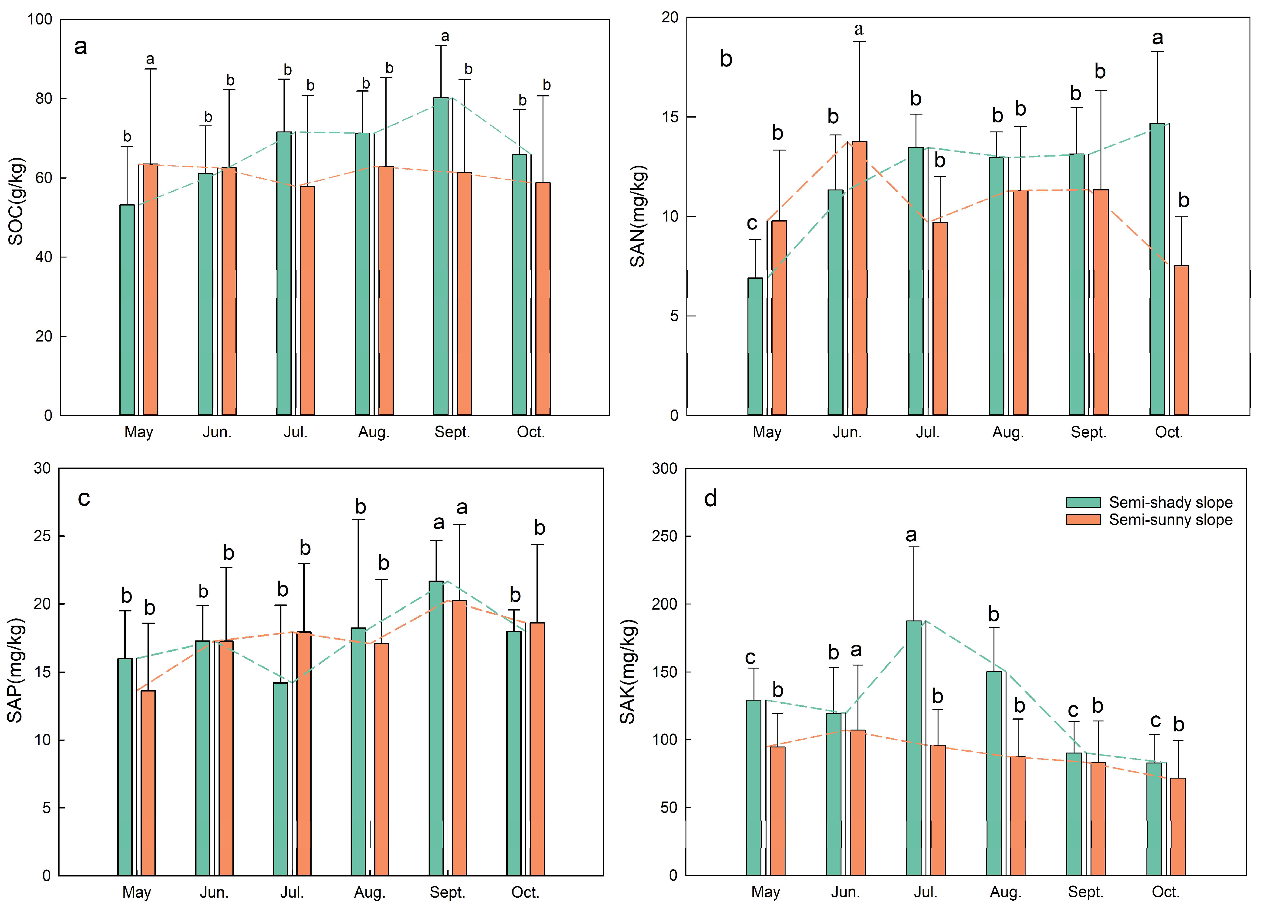
3.1. Temporal Variation in SOC and Soil Available Nutrients

3.1.1. Temporal Variation of SOC

The SOC contents of different slope orientations significantly differed during the growing season. During the growing season (Figure 4a), the SOC content on the semi-shady slope reached its highest value (80.20 g/kg) in September and its lowest value (53.17 g/kg) in May. Conversely, the SOC content on the semi-sunny slope reached its maximum value (63.43 g/kg) and minimum value (57.84 g/kg) in May and July, respectively. In September, on the semi-shady slope, and in May, on the semi-sunny slope, the SOC content was significantly different from that observed in other months (p < 0.05). Compared to the semi-sunny slope, the SOC content of the semi-shady slope was lower in May and June but was significantly higher from July to October.

3.1.2. Temporal Variation of Soil Available Nutrients

During the growing season (Figure 4b), the content of SAN reached its maximum value (14.67 mg/kg) in October and its minimum value (6.91 mg/kg) in May on the semi-shady slope; it reached its maximum value (13.75 mg/kg) in June and its minimum value (7.53 mg/kg) in October on the semi-sunny slope. On the semi-shady slope, the SAN content in October was significantly different from that in June, July, August, and September (p < 0.05) and more significantly different starting from May (p < 0.05). On the semi-sunny slope, the SAN content in June was significantly different from that in other months (p < 0.05). The SAN content on the semi-sunny slope was greater than that on the semi-shady slope from May to June, and the SAN content on the semi-shady slope was greater than that on the semi-sunny slope from July to October. The SAN content was consistent with the SOC content, indicating strong synchronization.

The SAP content reached its maximum value (21.67 mg/kg) in September and its minimum value (14.21 mg/kg) in July on the semi-shady slope (Figure 4c), and it also reached its maximum value (20.25 mg/kg) in September and its minimum value (13.63 mg/kg) in May on the semi-sunny slope. In September, the SAP content on both the semi-shady and semi-sunny slopes was significantly different from that in all other months of the growing season (p < 0.05). The SAP content on the semi-sunny slope was greater than that on the semi-shady slope in July and October, whereas the SAP content on the semi-shady slope was greater than that on the semi-sunny slope in other months.

The SAK content reached its maximum value (187.71 mg/kg) in July and its minimum value (83 mg/kg) in October on the semi-shady slope (Figure 4d); it reached its maximum value (107.13 mg/kg) in June and its minimum value (71.75 mg/kg) in October on the semi-sunny slope. On the semi-shady slope, the SAK content in July was significantly different from that in June and August (p < 0.05) and more significantly different from that in May, September, and October (p < 0.05). On the semi-sunny slope, the SAK content in June was significantly different from that in other months (p < 0.05), but the differences were not significant in other months. The SAK content of the semi-shady slope was consistently higher than that of the semi-sunny slope.

3.2. Spatial Variation of SOC and Soil Available Nutrients

3.2.1. Spatial Variability of SOC

Based on the soil profiles, the SOC content in different slope directions gradually decreased with the soil layer depth (Table 1), which is consistent with the results of existing studies [4,24]. For different slope directions, the SOC content was always higher in soil layers at depths of 0–10 cm, 10–20 cm, and 20–30 cm and tended to decrease gradually when going deeper into the soil layers. The SOC content in the soil layers at 0–10 cm, 10–20 cm, 20–30 cm, and 30–40 cm was greater on the semi-sunny slope than that on the semi-shady slope, whereas the SOC content on the semi-shady slope was greater than that on the semi-sunny slope in the soil layers at 40–50 cm and 50–60 cm.

3.2.2. Spatial Variability of Soil Available Nutrients

In the soil vertical profile (Table 1), the SAN content in different slope directions was higher in the surface layer than that in the deeper layers, which is consistent with the results of previous studies [36]. This result indicated the presence of high nitrogen content and high soil fertility in the surface layer. Except for a slight increase in the soil layer of 40–50 cm on the semi-shady slope and in the soil layer of 10–20 cm on the semi-sunny slope, the SAN content of the different slope directions presented an overall decreasing trend with an increase in soil depth. The SAN content on the semi-shady slope was greater than that on the semi-sunny slope in the soil layers of 0–10 cm, 20–30 cm, 40–50 cm, and 50–60 cm, while the SAN content on the semi-sunny slope was greater than that on the semi-shady slope in the soil layers of 10–20 cm and 30–40 cm.

With an increase in the soil layer depth, the SAP content variations for different slope directions were more complex, but all presented greater SAP content in the surface soil layers than in the deeper soil layers (Table 1). This result is consistent with the results obtained by Yang et al. [24] in the Qilian Mountains. On the semi-shady slope, the content of SAP decreased in the soil layers of 0–10 cm, 10–20 cm, 20–30 cm, and 30–40 cm and increased in the soil layers of 40–50 cm and 50–60 cm. On the semi-sunny slope, the content of SAP decreased in the soil layers of 0–10 cm, 10–20 cm, 40–50 cm, and 60–70 cm and increased in the soil layers of 20–30 cm, 30–40 cm, and 50–60 cm. The comparison showed that the content of SAP on the semi-shady slope was greater than that on the semi-sunny slope in the soil layers of 10–20 cm and 20–30 cm, while the SAP content on the semi-sunny slope was greater than that on the semi-shady slope in other soil layers.

For the different slope directions, the content of SAK was higher in the surface soil layers than in the deeper soil layers (Table 1). The vertical variation of the SAK content was consistent in different slope directions, with the SAK content decreasing in the soil layers of 0–10 cm, 10–20 cm, 20–30 cm, and 30–40 cm and increasing in the soil layers of 40–50 cm and 50–60 cm on the semi-shady slope. In addition, the SAK content was found to decrease in the soil layers of 0–10 cm, 10–20 cm, 20–30 cm, 30–40 cm, and 40–50 cm and increase in the soil layers of 50–60 cm, 60–70 cm, and 70–80 cm on the semi-sunny slope. Throughout the soil profile, the SAK content was consistently higher on the semi-shady slope than on the semi-sunny slope.

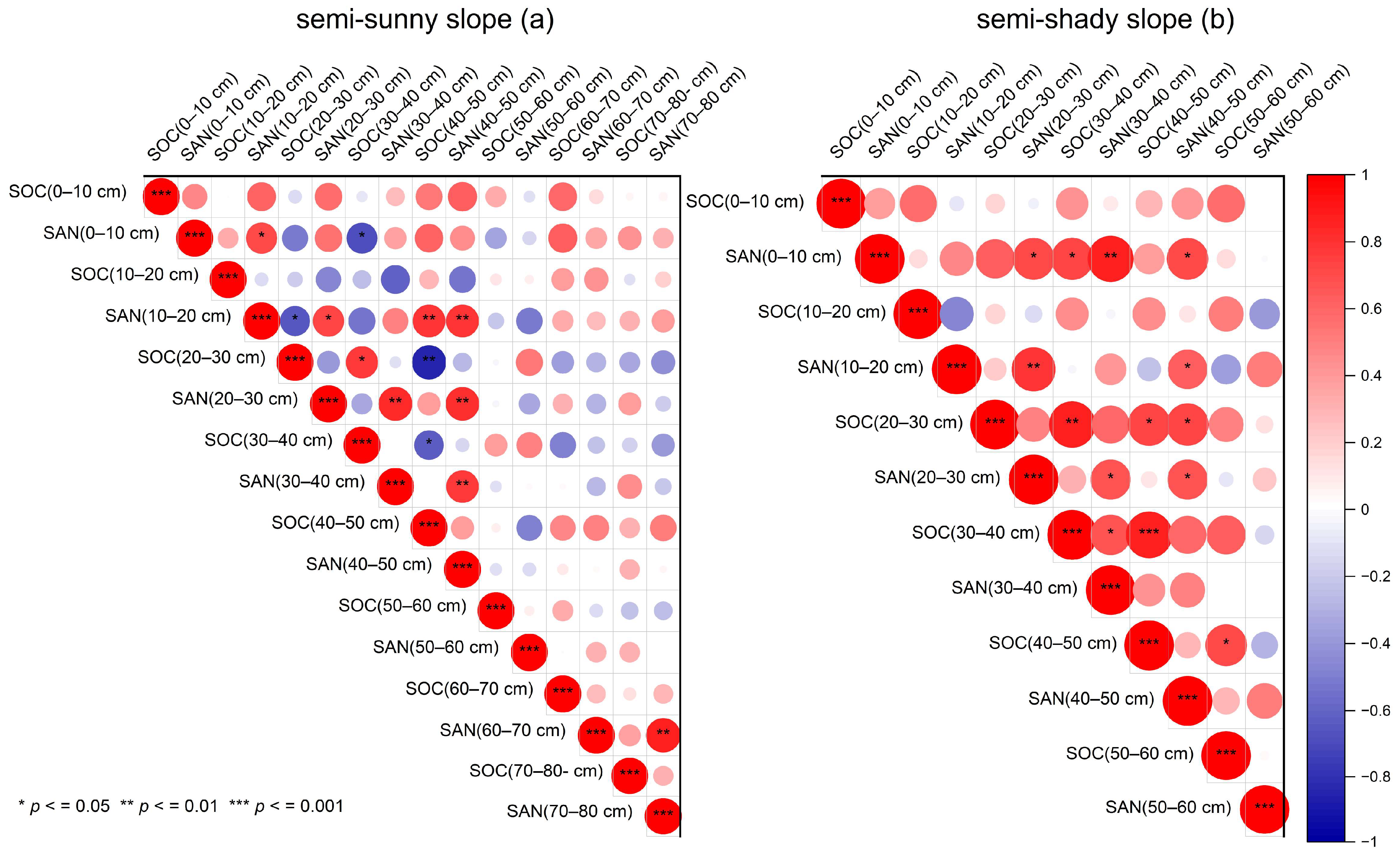
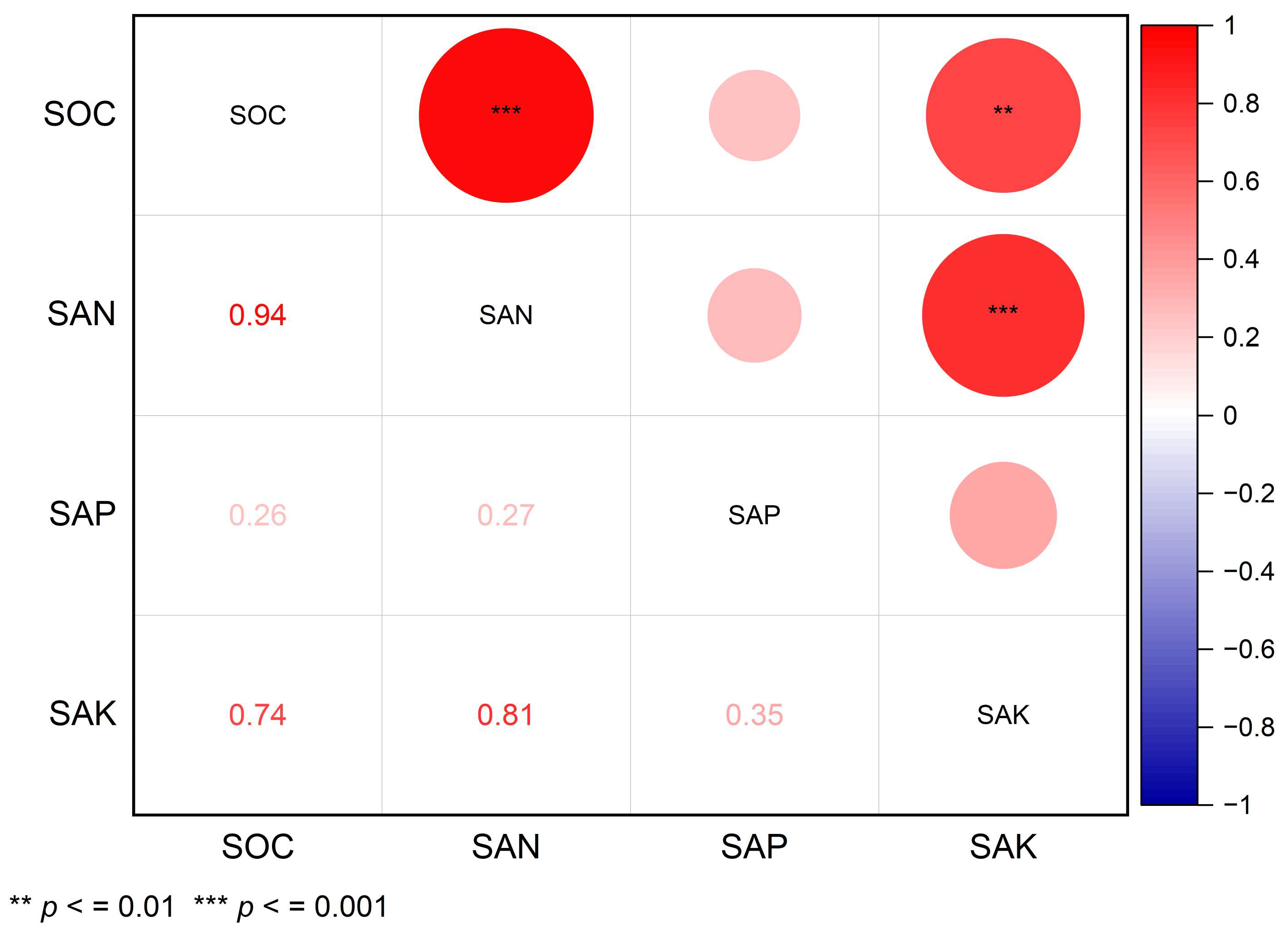
3.3. The Relationship between SOC and Soil Available Nutrients

3.3.1. The Relationship between SOC and SAN

The SOC content was significantly positively correlated with the SAN content in the study area during the whole growing season (p < 0.001) (Figure 5) [24]. However, the relationship between the SOC content and SAN content was different for different slope directions and soil depths (Figure 6). On the semi-shady slope, the SOC content was positively correlated with the SAN content in the soil layers of 0–10 cm, 20–30 cm, 30–40 cm, and 40–50 cm; significantly positively correlated in the soil layer of 30–40 cm (r = 0.67, p < 0.05); moderately positively correlated in the soil layer of 20–30 cm (r = 0.48); and not correlated in the soil layer of 50–60 cm. This result indicates that SAN is not sufficient to explain the controlling mechanisms underlying changes in the SOC content at the soil layer of 50–60 cm. Unlike in other soil layers, the SOC content was moderately negatively correlated with SAN content in the soil layer of 10–20 cm (r = −0.47). On the semi-sunny slope, the SOC content was moderately positively correlated in the soil layer of 0–10 cm (r = 0.47), and weakly positively correlated in soil layers of 40–50 cm (r = 0.39) and 70–80 cm (r = 0.31). The SOC content was moderately negatively correlated with the SAN content in the soil layers of 10–20 cm and 20–30 cm, which presented weaker correlations, but not correlated with SAN in the soil layers of 30–40 cm and 50–60 cm.

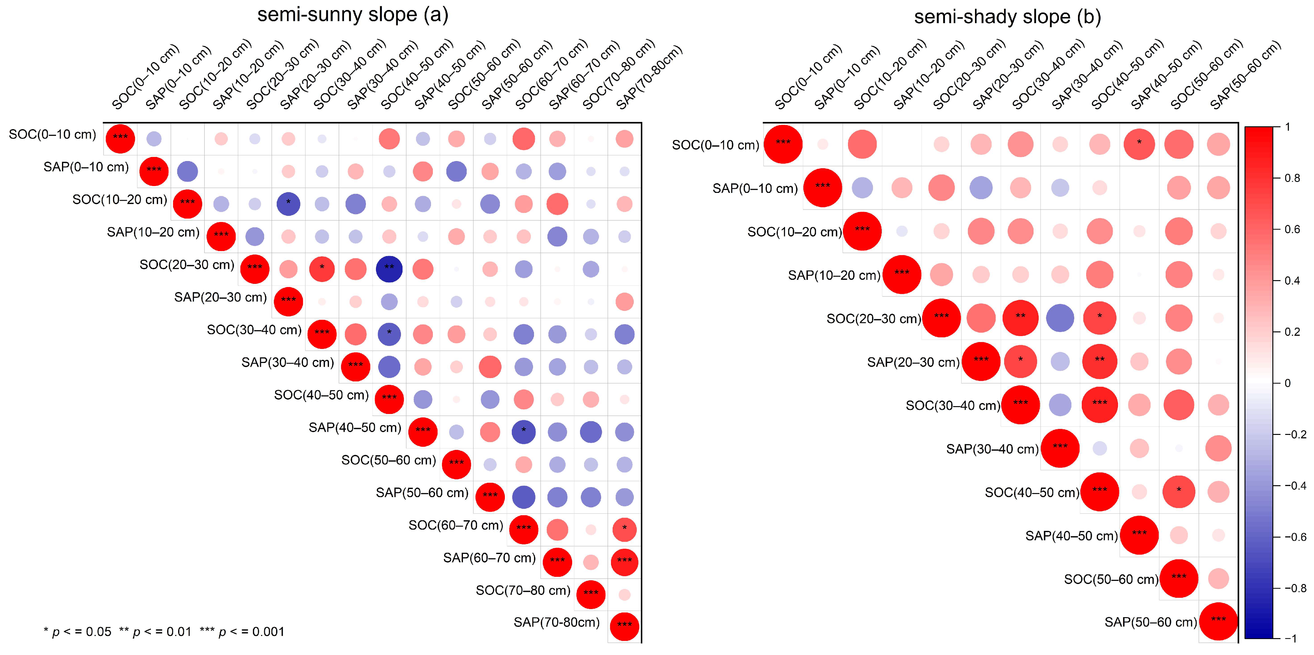
3.3.2. The Relationship between SOC and SAP

The SOC content was positively correlated with the SAP content during the whole growing season, but this correlation was not significant (Figure 5). As shown in Figure 7, the SOC content of the semi-shady slope had a moderate positive correlation with SAP in the soil layer of 20–30 cm (r = 0.55). In the soil layer of 30–40 cm, the SOC content on the semi-shady slope was also weakly negatively correlated with the SAP content (r = −0.34). In the soil layer of 10–20 cm, the SOC content was not significantly negatively correlated with the SAP content. On the semi-sunny slope, the SOC was negatively correlated with the SAP in the soil layers of 0–10 cm, 10–20 cm, 40–50 cm, and 50–60 cm and moderately negatively correlated in the soil layer of 40–50 cm (r = −0.41). In the soil layers of 20–30 cm, 30–40 cm, and 60–70 cm, the SOC content on the semi-sunny slope was positively correlated with the SAP content, with stronger correlation coefficients in the soil layers of 30–40 cm (r = 0.57) and 60–70 cm (r = 0.55). This result indicates that the accumulation of SOC and SAP was somewhat synchronous, with both the SOC content and the SAP content observed to decrease with an increase in soil depth and showing a positive correlation.

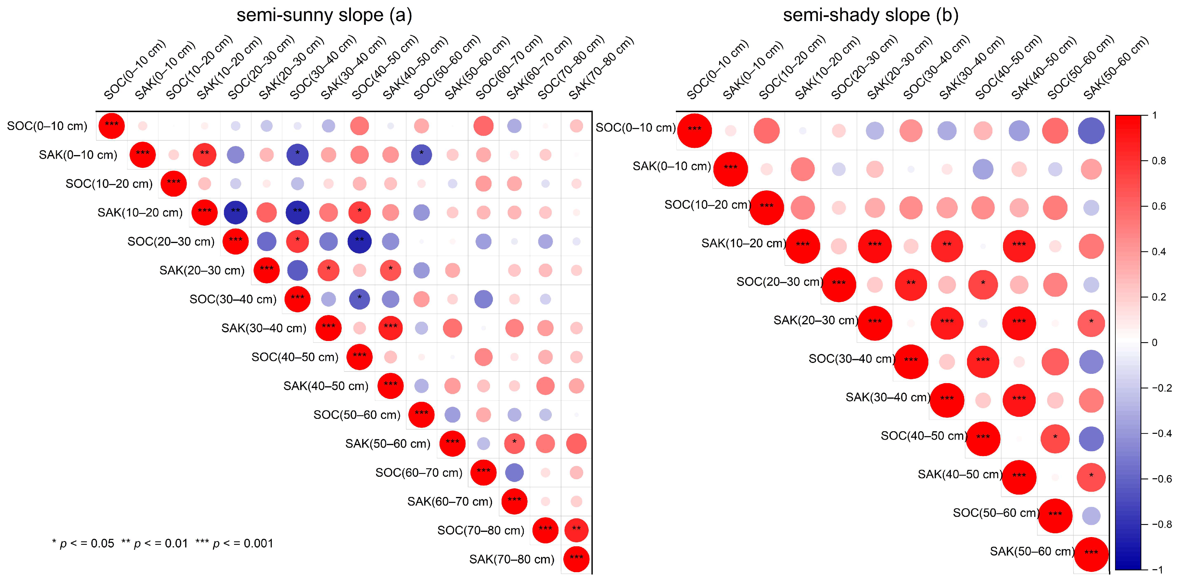
3.3.3. The Relationship between SOC and SAK

The SOC content was significantly positively correlated with the SAK content in the study area during the whole growing season (p < 0.001) (Figure 5). As shown in Figure 8, the SOC content was positively correlated with the SAK content in the soil layers of 10–20 cm, 20–30 cm, and 30–40 cm on the semi-shady slope, with a moderately positive correlation for the soil layer of 10–20 cm (r = 0.48). There was a significant positive correlation with the SAK content in the soil layer of 70–80 cm on the semi-sunny slope (r = 0.84, p < 0.05). On the semi-shady slope, the SOC content was weakly negatively correlated with the SAK content in the soil layer of 50–60 cm (r = 0.29). On the semi-sunny slope, the SOC was also negatively correlated with the SAN in the soil layers of 20–30 cm, 30–40 cm, 50–60 cm, and 60–70 cm, with moderate negative correlations in the soil layers of 20–30 cm (r = −0.56) and 60–70 cm (r = −0.52).

4. Discussions

4.1. Impact of Slope Orientation and Soil Layer Depth on the SOC and Soil Available Nutrient

The variability of environmental factors across different slope directions directly impacts soil temperature, vegetation type, soil moisture, etc. In the study area, under the same vegetation type, variations in temperature and soil moisture content resulting from differences in slope orientation were identified as the primary factors influencing the levels of SOC and soil available nutrients. These variations have a direct influence on the rate of SOC mineralization and indirectly affect the accumulation of SOC and soil available nutrients. Compared to that on the semi-sunny slope, the SOC content on the semi-shady slope was lower in May and June but significantly increased from July to October (Figure 4a). Studies have shown that temperature and precipitation are positively correlated with SOC reserves on a global scale [4]. In high-altitude areas, temperature is a limiting factor for vegetation growth [18]. Increased temperature increases microorganism decomposition rates, which accelerates decreases in SOC content [3]. In July, the semi-sunny slope was influenced by greater precipitation and a higher temperature (Figure 2). These factors increased soil respiration and accelerated the decomposition and transformation of SOM, which was not conducive to the accumulation of SOC on the semi-sunny slope. In September, in the study area, the temperature dropped, and precipitation increased, but the semi-shady slope retained a higher soil moisture content (87.51%) (Figure 9). This factor weakened the soil’s microbial activity and preserved a large amount of organic matter in the soil, which resulted in a relatively higher SOC content on the semi-shady slope. In addition, throughout the soil profile, the SAK content was consistently higher on the semi-shady slope than on the semi-sunny slope (Table 1), which may be related to the soil moisture content affecting the release and fixation of potassium. It was previously shown that SAK content has a significant negative correlation with soil moisture [2]. According to Table 1, the soil moisture content in the study area was consistently higher on the semi-sunny slope than on the semi-shady slope, resulting in a lower SAK content on the former compared to the latter.

Variations in soil depth directly impact soil moisture content, soil texture, vegetation apomixis, and variability in plant root systems. Indirectly, these variations also affect the accumulation of SOC and the content of soil available nutrients. The higher the soil clay content, the better the water retention capacity, growth of surface vegetation, vegetation litter, and organic matter of the surface soil [37]. Although this paper lacked sampling data on the root systems of vegetation in the study area, Zhang et al. [38] previously reported that the root systems of subalpine scrub vegetation are predominantly distributed within the 0–30 cm soil layer. The surface soil has a high SOC content due to the distribution of vegetation roots and the accumulation of litter [39]. Research has shown that the thickness of the vegetation litter has a negative correlation with the soil bulk density (BD) [40]. In comparison to the semi-shady slope, the semi-sunny slope had a smaller BD in the soil layer of 0–10 cm (Table 1), resulting in a thicker vegetation litter and a higher input of SOC content. However, the size of the litter and vegetation root distribution decreases with an increase in soil depth, so the SOC content also decreases gradually. In addition, the SOC content is related to many factors at the same soil depth on different slope directions, such as temperature, precipitation, illumination, soil clay content, and vegetation biomass, which affect the spatial distribution patterns of SOC [2]. In the study area, the light conditions, surface soil moisture content, and clay content (Table 1) were better on the semi-sunny slope than on the semi-shady slope [31], and the plant root system had a positive correlation with the soil moisture content [41], resulting in a higher distribution of plant roots and a greater amount of biomass accumulated by the vegetation on the semi-sunny slope. Therefore, the SOC content in the soil layers of 0–10 cm, 10–20 cm, 20–30 cm, and 30–40 cm was higher on the semi-sunny slope than on the semi-shady slope. With an increase in soil depth, a large amount of SOM was accumulated and preserved since the evaporation of soil moisture weakened. Moreover, the decomposition rate of SOM was relatively slow on the semi-shady slope, which led to the significant accumulation and preservation of SOC. Therefore, the SOC content in the soil layers of 40–50 cm and 50–60 cm was higher on the semi-shady slope than on the semi-sunny slope. The level of soil available nutrient content represents the intensity of nutrients that the soil can supply for vegetation growth [9]. The available nutrient content for the different slope directions was highest in the soil layer of 0–10 cm and showed a decreasing trend with an increase in soil depth, indicating that the surface aggregation of soil available nutrients was significant. In the study area, most of the vegetation roots were concentrated in the soil layer of 0–30 cm [38], so the accumulation of soil available nutrients in the surface layer can provide the required nutrients for vegetation growth. This outcome was consistent with the results obtained by Tudi et al. [14] in the Tianshan Mountains of Northwestern China.

4.2. Impact of Slope Orientation and Soil Layer Depth on the Relationship between SOC and Soil Available Nutrient

A variation in slope orientation affects the relationship between SOC and soil available nutrients. For instance, on the semi-shady slope, there was a significant positive correlation between the SAN content and the SOC content in the soil layer of 30–40 cm. However, this correlation was negligible in the same soil layer on the semi-sunny slope. These findings suggest that SAN had a limited impact on the variation in the SOC content in the soil layer of 30–40 cm on the semi-sunny slope. Interestingly, the correlation between the SOC content and the SAN content was higher in the same soil layer on the semi-shady slope than on the semi-sunny slope (Figure 6). This result could be attributed to the weaker evaporation and higher soil moisture content (as indicated in Table 1) on the semi-shady slope, which facilitated the accumulation of SAN content. The relationship between the SOC content and the SAP content was more significant on the semi-sunny slope than on the semi-shady slope (Figure 7). Phosphorus produced by vegetation growth mainly comes from the soil, with vegetation root activity directly or indirectly influencing the changes in the SAP content. Moreover, the presence of vegetation roots at different soil depths can accelerate the soil phosphorus cycle [42]. Therefore, the presence of more phosphorus in the soil promotes vegetation growth and contributes to vegetation photosynthesis, which, in turn, affects the SOC content. The growth of vegetation on the semi-sunny slope was better than that on the semi-shady slope, with a large amount of vegetation litter accumulating on the surface. The root system of the subalpine scrubs in the study area was shallowly distributed [38], which led to the vigorous root growth of the corresponding vegetation [41]. This growth increased SOC input and resulted in a higher correlation between the SOC content and the SAP content on the semi-sunny slope. The correlation between the SAK content and the SOC content was more significant on the semi-sunny slope than on the semi-shady slope, which was consistent with the correlation between the SOC content and the SAP content.

The correlation between SOC and soil available nutrients exhibited variations across different depths within the soil profile. For example, in the case of the semi-sunny slope, the SOC content was moderately and positively correlated with SAN in the soil layer of 0–10 cm (r = 0.47) because SAN is the main form in which plants obtain nitrogen directly from the soil [43]. The soil nitrogen content is mostly attributed to the return of vegetation litter and roots, organic matter formed by microbial decomposition and synthesis, artificial fertilization, etc. [20]. However, the study area belongs to the subalpine scrub area, where vegetation growth is weakly disturbed by anthropogenic factors (e.g., slight grazing activity), so the content of SAN is only related to the content and quality of the SOM [44]. It was shown that the SAN content increases with an increase in the SOC content [36], while soil nitrogen mainly contributes to the decomposition of organic matter through microbial activity and vegetation growth [45]. Since vegetation litter and plant roots are primarily distributed in the surface layer of the soil [38], the correlation between SOC and SAN is more apparent than other relationships. In the semi-sunny slope, there was a moderate and negative correlation observed between SOC and SAP in the soil layer of 40–50 cm because the SOC content decreased as SAP increased (due to the reduced consumption of SAP by the plants) in this soil layer. This result is similar to previous research findings [20]. We also observed a significant positive correlation with the SAK content in the soil layer of 70–80 cm on the semi-sunny slope (r = 0.84, p < 0.05) (Figure 8), possibly due to the influence of the mineral composition of the parent rock. This finding was consistent with the results obtained by Liu et al. [16] in forestlands. SAK is mainly influenced by land type, soil-forming parent material, soil texture, topography, and hydrology [20,46], and its main sources include the mineralization of the vegetation litter and the weathering of minerals in the parent layer [20,47]. Therefore, deeper soils are most strongly affected by SAK because SAK is associated with the weathering of the parent layer’s materials. High-potassium soils are supplied by high-potassium-bearing minerals, such as mica and feldspar, in the soil parent materials [2]. This phenomenon was also reported by Li et al. [48], who demonstrated SAK content to be highest in sandstone residual slope deposits, moderate in the Quaternary alluvium, and lowest in granite residual slope deposits. The soils in the study area included sandstone weathering deposits, which also contained more SAK.

5. Conclusions

Based on soil samples collected from the semi-sunny slope and the semi-shady slope in the subalpine shrub zone of the eastern Qilian Mountains from May to October 2019, we analyzed the temporal and spatial changes in SOC and soil available nutrients and their relationships. Some conclusions as provided below.

The SOC content and soil available nutrients were mainly located on the semi-shady slope rather than the semi-sunny slope during the growing season, and they decreased as the soil depth increased in different slope directions, which showed obvious surface aggregation. At the same soil depth, the SOC content on the semi-sunny slope was greater than that on the semi-shady slope in the soil layers of 0–40 cm and was greater on the semi-shady slope than on the semi-sunny slope in the soil layers of 40–60 cm.

The SOC content was significantly positively correlated with soil available nutrient contents in the study area. However, the correlation between SOC and soil available nutrients varied among different soil layers and slope orientations. For example, the SOC content was more obviously correlated with the SAN content in the soil layer of 30–40 cm (r = 0.67, p < 0.05) on the semi-shady slope; the SOC content was more obviously correlated with the SAP content in the soil layers of 30–40 cm (r = 0.57) and 60–70 cm (r = 0.55) on the semi-sunny slope; and the SOC content was more obviously correlated with the SAK content in the soil layer of 70–80 cm (r = 0.84) on the semi-sunny slope.

The variability of environmental factors across different slope directions directly impacts soil temperature, vegetation type, soil moisture, etc. These variations have a direct influence on the rate of SOC mineralization and indirectly affect the accumulation of SOC and soil available nutrients. The SOC content is closely related to soil available nutrients. Therefore, the present results indicate a significant positive correlation between SOC and soil available nutrients. Furthermore, the results show the significant influence of different slope directions and soil layers on their spatial distributions and interrelationships. These findings provide a theoretical foundation for studying the carbon stock and carbon cycle in high-altitude regions.

References

1. Wan, Q.; Zhu, G.; Guo, H.; Zhang, Y.; Pan, H.; Yong, L.; Ma, H. Influence of vegetation coverage and climate environment on soil organic carbon in the Qilian Mountains. Sci. Rep. 2019, 9, 17623. [Google Scholar] [CrossRef]
2. Tian, L.M.; Zhao, L.; Wu, X.D.; Fang, H.B.; Zhao, Y.H.; Yue, G.Y.; Liu, G.M.; Chen, H. Vertical patterns and controls of soil nutrients in alpine grassland: Implications for nutrient uptake. Sci. Total Environ. 2017, 607–608, 855–864. [Google Scholar] [CrossRef]
3. Chen, L.F.; He, Z.B.; Du, J.; Zhang, J.J.; Zhu, X. Patterns and environmental controls of soil organic carbon and total nitrogen in alpine ecosystems of northwestern China. Catena 2016, 137, 37–43. [Google Scholar] [CrossRef]
4. Jobbágy, E.G.; Jackson, R.B. The vertical distribution of soil organic carbon and its relation to climate and vegetation. Ecol. Appl. 2000, 10, 423–436. [Google Scholar] [CrossRef]
5. Wei, J.B.; Xiao, D.N.; Zhang, X.Y.; Li, X.Y. Topography and land use effects on the spatial variation of soil organic carbon: A case study in a typical small watershed of the black soil region in northeast China. Eurasian Soil Sci. 2008, 41, 39–47. [Google Scholar] [CrossRef]
6. Bennie, J.; Huntley, B.; Wiltshire, A.; Hill, M.O.; Baxter, R. Slope, aspect and climate: Spatially explicit and implicit models of topographic microclimate in chalk grassland. Ecol. Modell. 2008, 216, 47–59. [Google Scholar] [CrossRef]
7. Huang, Y.M.; Liu, D.; An, S.S. Effects of slope aspect on soil nitrogen and microbial properties in the Chinese Loess region. Catena 2015, 125, 135–145. [Google Scholar] [CrossRef]
8. Xu, X.; Zhou, Y.; Ruan, H.; Luo, Y.; Wang, J. Temperature sensitivity increases with soil organic carbon recalcitrance along an elevational gradient in the Wuyi Mountains, China. Soil Biol. Biochem. 2010, 42, 1811–1815. [Google Scholar] [CrossRef]
9. Post, W.M.; Emanuel, W.R.; Zinke, P.J.; Stangenberger, A.G. Soil carbon pools and world life zones. Nature 1982, 298, 156–159. [Google Scholar] [CrossRef]
10. Nie, X.; Peng, Y.; Li, F.; Yang, L.C.; Xiong, F.; Li, C.B.; Zhou, G.Y. Distribution and controlling factors of soil organic carbon storage in the northeast Tibetan shrublands. J. Soils Sediment 2019, 19, 322–331. [Google Scholar] [CrossRef]
11. Makarov, M.I.; Malysheva, T.I.; Menyailo, O.V. Isotopic composition of nitrogen and transformation of nitrogen compounds in meadow-alpine soils. Eurasian Soil Sci. 2019, 52, 1028–1037. [Google Scholar] [CrossRef]
12. Makarov, M.I.; Glaser, B.; Zech, W.; Malysheva, T.I.; Bulatnikova, I.V.; Volkov, A.V. Nitrogen dynamics in alpine ecosystems of the northern Caucasus. Plant Soil 2003, 256, 389–402. [Google Scholar] [CrossRef]
13. Oduor, C.O.; Karanja, N.K.; Onwonga, R.N.; Mureithi, S.M.; Pelster, D.; Nyberg, G. Enhancing soil organic carbon, particulate organic carbon and microbial biomass in semi-arid rangeland using pasture enclosures. BMC Ecol. 2018, 18, 45. [Google Scholar] [CrossRef] [PubMed]
14. Tudi, M.; Li, H.Y.; Li, H.; Wang, L.; Yang, L.; Tong, S.M.; Yu, Q.M.; Ruan, H.D. Evaluation of soil nutrient characteristics in Tianshan Mountains, North-western China. Ecol. Indic. 2022, 143, 10943. [Google Scholar] [CrossRef]
15. Shao, W.; Wang, Q.; Guan, Q.; Luo, H.; Ma, Y.; Zhang, J. Distribution of soil available nutrients and their response to environmental factors based on path analysis model in arid and semi-arid area of northwest China. Sci. Total Environ. 2022, 827, 154254. [Google Scholar] [CrossRef]
16. Liu, L.; Wang, H.; Dai, W.; Lei, X.; Yang, X.; Li, X. Spatial variability of soil organic carbon in the forestlands of northeast China. J. For. Res. 2014, 25, 867–876. [Google Scholar] [CrossRef]
17. Wang, H.; Li, J.; Zhang, Q.; Liu, J.; Yi, B.; Li, Y.; Wen, J.; Di, H. Grazing and enclosure alter the vertical distribution of organic nitrogen pools and bacterial communities in semiarid grassland soils. Plant Soil 2019, 439, 525–539. [Google Scholar] [CrossRef]
18. He, Z.; Zhao, W.; Zhang, L.; Liu, H. Response of tree recruitment to climatic variability in the alpine treeline ecotone of the Qilian Mountains, northwestern China. Forest Sci. 2013, 59, 118–126. [Google Scholar] [CrossRef]
19. Tan, D.; Jin, J.; Jiang, L.; Huang, S.; Liu, Z. Potassium assessment of grain-producing soils in North China. Agric. Ecosyst. Environ. 2012, 148, 65–71. [Google Scholar] [CrossRef]
20. Li, T.; Liang, J.; Chen, X.; Wang, H.; Zhang, S.; Pu, Y.; Xu, X.; Li, H.; Po, X.; Liu, X. The interacting roles and relative importance of climate, topography, soil properties and mineralogical composition on soil potassium variations at a national scale in China. Catena 2021, 196, 104875. [Google Scholar] [CrossRef]
21. Wang, J.L.; Ou, Y.H.; Wang, Z.H.; Chang, T.J.; Li, P.; Shen, Z.X.; Zhong, Z.M. Influential factors and distribution characteristics of topsoil organic carbon in alpine grassland ecosystem in the south slope of Gunga South Mountain-La Ruigangri Mountain. Chin. J. Soil Sci. 2010, 41, 346–350. [Google Scholar]
22. Cong, S.; Zhou, D.; Li, Q.; Huang, Y. Effects of Fencing on Vegetation and Soil Nutrients of the Temperate Steppe Grasslands in Inner Mongolia. Agronomy 2021, 11, 1546. [Google Scholar] [CrossRef]
23. Wu, X.; Wang, L.; An, J.; Wang, Y.; Song, H.; Wu, Y.; Liu, Q. Relationship between Soil Organic Carbon, Soil Nutrients, and Land Use in Linyi City (East China). Sustainability 2022, 14, 13585. [Google Scholar] [CrossRef]
24. Yang, L.; Jia, W.; Shi, Y.; Zhang, Z.Y.; Xiong, H.; Zhu, G.F. Spatiotemporal Differentiation of Soil Organic Carbon of Grassland and Its Relationship with Soil Physicochemical Properties on the Northern Slope of Qilian Mountains, China. Sustainability 2020, 12, 9396. [Google Scholar] [CrossRef]
25. Qin, Y.; Feng, Q.; Holden, N.M.; Cao, J. Variation in soil organic carbon by slope aspect in the middle of the Qilian Mountains in the upper Heihe River Basin, China. Catena 2016, 147, 308–314. [Google Scholar] [CrossRef]
26. Zhu, M.; Feng, Q.; Qin, Y.; Cao, J.; Zhang, M.; Liu, W.; Deo, R.C.; Zhang, C.; Li, R.; Li, B. The role of topography in shaping the spatial patterns of soil organic carbon. Catena 2019, 176, 296–305. [Google Scholar] [CrossRef]
27. Yang, R.; Su, Y.; Wang, M.; Wang, T.; Yang, X.; Fan, G.; Wu, T. Spatial pattern of soil organic carbon in desert grasslands of the diluvial-alluvial plains of northern Qilian Mountains. J. Arid Land 2014, 6, 136–144. [Google Scholar] [CrossRef]
28. Zhou, J.; Xue, D.; Lei, L.; Wang, L.; Zhong, G.; Liu, C.; Xiang, J.; Huang, M.; Feng, W.; Li, Q. Impacts of Climate and Land Cover on Soil Organic Carbon in the Eastern Qilian Mountains, China. Sustainability 2019, 11, 5790. [Google Scholar] [CrossRef]
29. Zhu, G.; Liu, Y.; Wang, L.; Sang, L.; Zhao, K.; Zhang, Z.; Lin, X.; Qiu, D. The isotopes of precipitation have climate change signal in arid Central Asia. Glob. Planet Change 2023, 225, 104103. [Google Scholar] [CrossRef]
30. Cao, B. Changes in Modern Glaciation at Lenglongling in the Eastern Part of the Qilian Mountains. Master’s Thesis, Lanzhou University, Gansu, China, 2013. [Google Scholar]
31. Wang, X.L. A Study on Mountain Climate in the Basin of Xiying River at the East Section of Qilian Mountains. Master’s Thesis, Lanzhou University, Gansu, China, 2008. [Google Scholar]
32. International Union of Soil Sciences (IUSS) Working Group WRB. World reference base for soil resources 2014, update 2015. In International Soil Classification System for the Designation of Soils and the Creation of Symbols for Soil Maps; Reports on World Soil Resources No. 106; FAO: Rome, Italy, 2015. [Google Scholar]
33. Lei, C.Y.; Li, W.; Yin, X.K.; Yuan, H.Y.; Wu, J.L. Study on the Relationship between Process of Critical Zone and Natural Ecological Restoration in the Qilian Mountains. Bul. Min. Petrol. Geochem. 2020, 39, 741–753. [Google Scholar]
34. Zhu, M.; Feng, Q.; Qin, Y.; Cao, J.; Li, H.; Zhao, Y. Soil organic carbon as functions of slope aspects and soil depths in a semiarid alpine region of Northwest China. Catena 2017, 152, 94–102. [Google Scholar] [CrossRef]
35. Xiao, Y.; Zhao, Y.; Tu, Z.D.; Qian, B.; Chang, R.M. Topology checking method for low voltage distribution network based on improved Pearson correlation coefficient. Power Syst. Prot. Control 2019, 47, 37–43. [Google Scholar]
36. Verma, T.P.; Moharana, P.C.; Naitam, R.K.; Meena, R.L.; Kumar, S.; Singh, R.; Tailor, B.L.; Singh, R.S.; Singh, S.K. Impact of cropping intensity on soil properties and plant available nutrients in hot arid environment of North-Western India. J. Plant Nutr. 2017, 40, 2872–2888. [Google Scholar] [CrossRef]
37. Li, Q.; Wang, L.; Fu, Y.; Lin, D.; Hou, M.; Li, X.; Hu, D.; Wang, Z. Transformation of soil organic matter subjected to environmental disturbance and preservation of organic matter bound to soil minerals: A review. J. Soils Sediments 2023, 23, 1485–1500. [Google Scholar] [CrossRef]
38. Zhang, F.H.; Jia, W.X.; Zhu, G.F.; Zhang, Z.Y.; Shi, Y.; Yang, L.; Xiong, H.; Zhang, M.M. Using stable isotopes to investigate differences of plant water sources in subalpine habitats. Hydrol. Process. 2022, 36, e14518. [Google Scholar] [CrossRef]
39. McDowell, R.W.; Nash, D.M.; Robertson, F. Sources of phosphorus lost from a grazed pasture receiving simulated rainfall. J. Environ. Qual. 2007, 36, 1281–1288. [Google Scholar] [CrossRef] [PubMed]
40. Wang, B.; Liu, D.; Yang, J.; Zhu, Z.; Darboux, F.; Jiao, J.; An, S. Effects of forest floor characteristics on soil labile carbon as varied by topography and vegetation type in the Chinese Loess Plateau. Catena 2021, 196, 104825. [Google Scholar] [CrossRef]
41. Okada, K.I.; Aiba, S.I.; Kitayama, K. Influence of temperature and soil nitrogen and phosphorus availabilities on fine-root productivity in tropical rainforests on Mount Kinabalu, Borneo. Ecol. Res. 2017, 32, 145–156. [Google Scholar] [CrossRef]
42. Chen, C.; Fang, X.; Xiang, W.; Lei, P.F.; Ouyang, S.; Kuzyakov, Y. Soil-plant co-stimulation during forest vegetation restoration in a subtropical area of southern China. For. Ecosyst. 2020, 7, 32. [Google Scholar] [CrossRef]
43. He, Y.; Sun, J.; Xiong, J.; Shang, H.; Wang, X. Patterns, Dynamics, and Drivers of Soil Available Nitrogen and Phosphorus in Alpine Grasslands across the QingZang Plateau. Remote Sens. 2022, 14, 4929. [Google Scholar] [CrossRef]
44. Yuan, L.; Gabriel, Y.K.M.; Timothy, J.C.; David, W. Organic matter contributions to nitrous oxide emissions following nitrate addition are not proportional to substrate-induced soil carbon priming. Sci. Total Environ. 2022, 851, 158274. [Google Scholar]
45. Sistla, S.A.; Asao, S.; Schimel, J.P. Detecting microbial N-limitation in tussock tundra soil: Implications for Arctic soil organic carbon cycling. Soil Biol. Biochem. 2012, 55, 78–84. [Google Scholar] [CrossRef]
46. Augusto, L.; Achat, D.L.; Jonard, M.; Vidal, D.; Ringeval, B. Soil parent material—A major driver of plant nutrient limitations in terrestrial ecosystems. Glob. Chang. Biol 2017, 23, 3808–3824. [Google Scholar] [CrossRef] [PubMed]
47. Tian, L.; Zhao, L.; Wu, X.; Hu, G.; Fang, H.; Zhao, Y.; Sheng, Y.; Chen, J.; Wu, J.C.; Li, W.P.; et al. Variations in soil nutrient availability across Tibetan grassland from the 1980s to 2010s. Geoderma 2019, 338, 197–205. [Google Scholar] [CrossRef]
48. Li, T.; Zhang, S.R.; Zhang, L.; Li, Y.; Gan, W.Z. Influence of soil potassium in zoology fragile areas of the northern Transverse Mountains. J. Soil Water Conserv. 2006, 20, 102–105. [Google Scholar]
Figure 1. Location of Qilian Mountain and distribution of sampling plots.
Sustainability 15 13028 g001
Figure 2. Monthly variation in temperature and precipitation in the study area. The red line represents the monthly average temperature, and the blue bar represents the monthly cumulative precipitation.
Sustainability 15 13028 g002
Figure 3. Photographs of the sampling sites at the beginning of monitoring (taken during sampling).
Sustainability 15 13028 g003
Figure 4. Temporal changes in SOC (a) and soil available nutrients (b-SAN; c-SAP; d-SAK) for different slope orientations. Different lowercase letters indicate significant differences in SOC and soil available nutrients among different months based on an LSD test (p < 0.05). The same lowercase letter indicates no significant differences in SOC or soil available nutrients between different months based on an LSD test (p < 0.05). The green and orange dashed lines represent line charts depicting the changes in SOC and soil available nutrients across different months.
Sustainability 15 13028 g004
Figure 5. Relationship between SOC content and soil available nutrient contents in the study area. The red color indicates a positive correlation between SOC and soil available nutrients, while the blue color indicates a negative correlation. The darker the color and the larger the circle, the greater the correlation coefficient and the stronger the correlation.
Sustainability 15 13028 g005
Figure 6. Relationship between SOC content and SAN content in different slope directions and soil depths. The red color indicates a positive correlation between SOC and SAN, while the blue color indicates a negative correlation. The darker the color and the larger the circle, the greater the correlation coefficient and the stronger the correlation.
Sustainability 15 13028 g006
Figure 7. Relationship between SOC content and SAP content for different slope directions and soil depths. The red color indicates a positive correlation between SOC and SAP, while the blue color indicates a negative correlation. The darker the color and the larger the circle, the greater the correlation coefficient and the stronger the correlation.
Sustainability 15 13028 g007
Figure 8. Relationship between SOC content and SAK content for different slope directions and soil depths. The red color indicates a positive correlation between SOC and SAK, while the blue color indicates a negative correlation. The darker the color and the larger the circle, the greater the correlation coefficient and the stronger the correlation.
Sustainability 15 13028 g008
Figure 9. Monthly variation in soil moisture content for different slope directions.
Sustainability 15 13028 g009