
Soft Computing and Machine Learning-Based Models to Predict the Slump and Compressive Strength of Self-Compacted Concrete Modified with Fly Ash


Abstract
:1. Introduction
Research Objectives
- I.
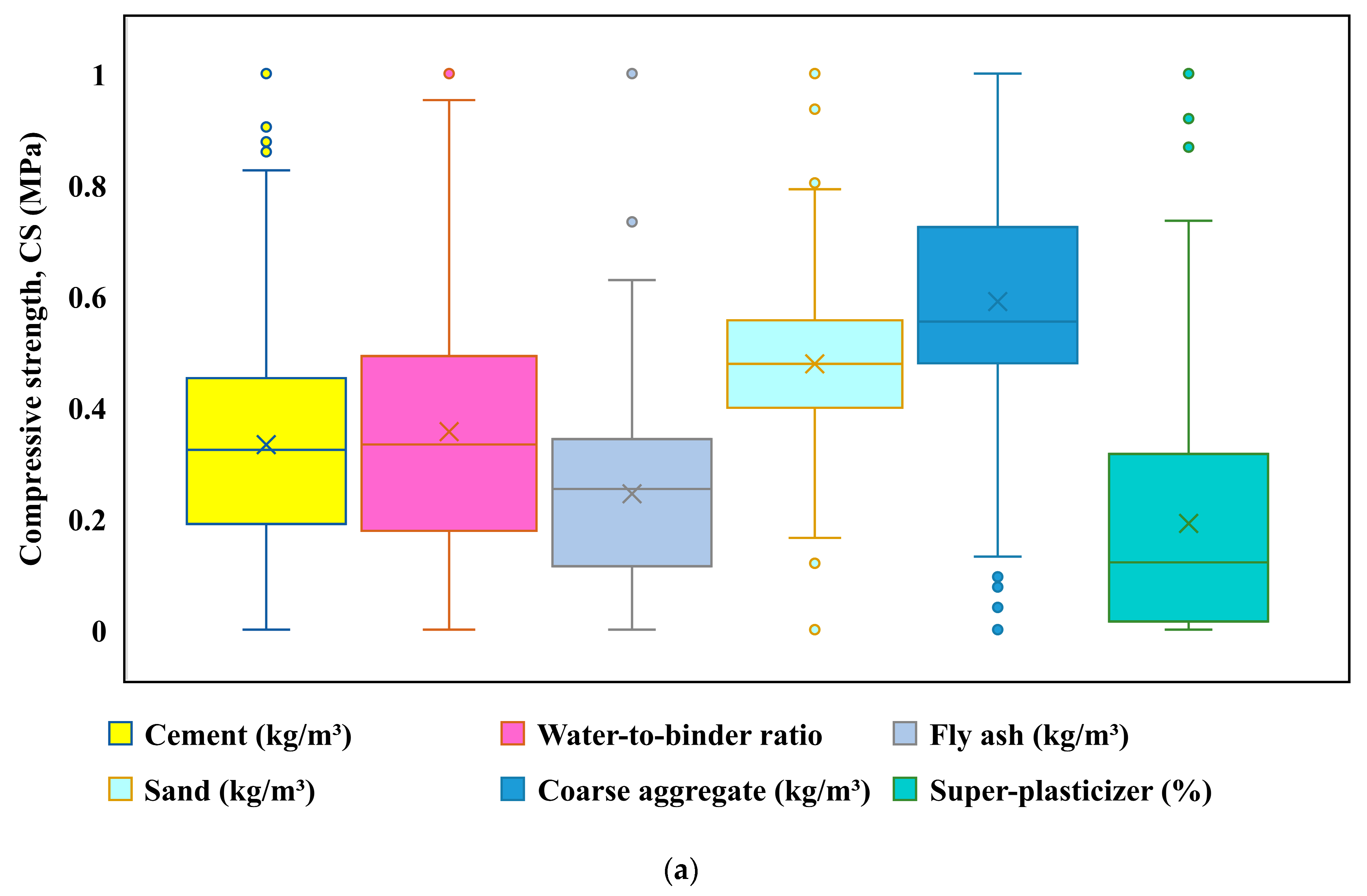
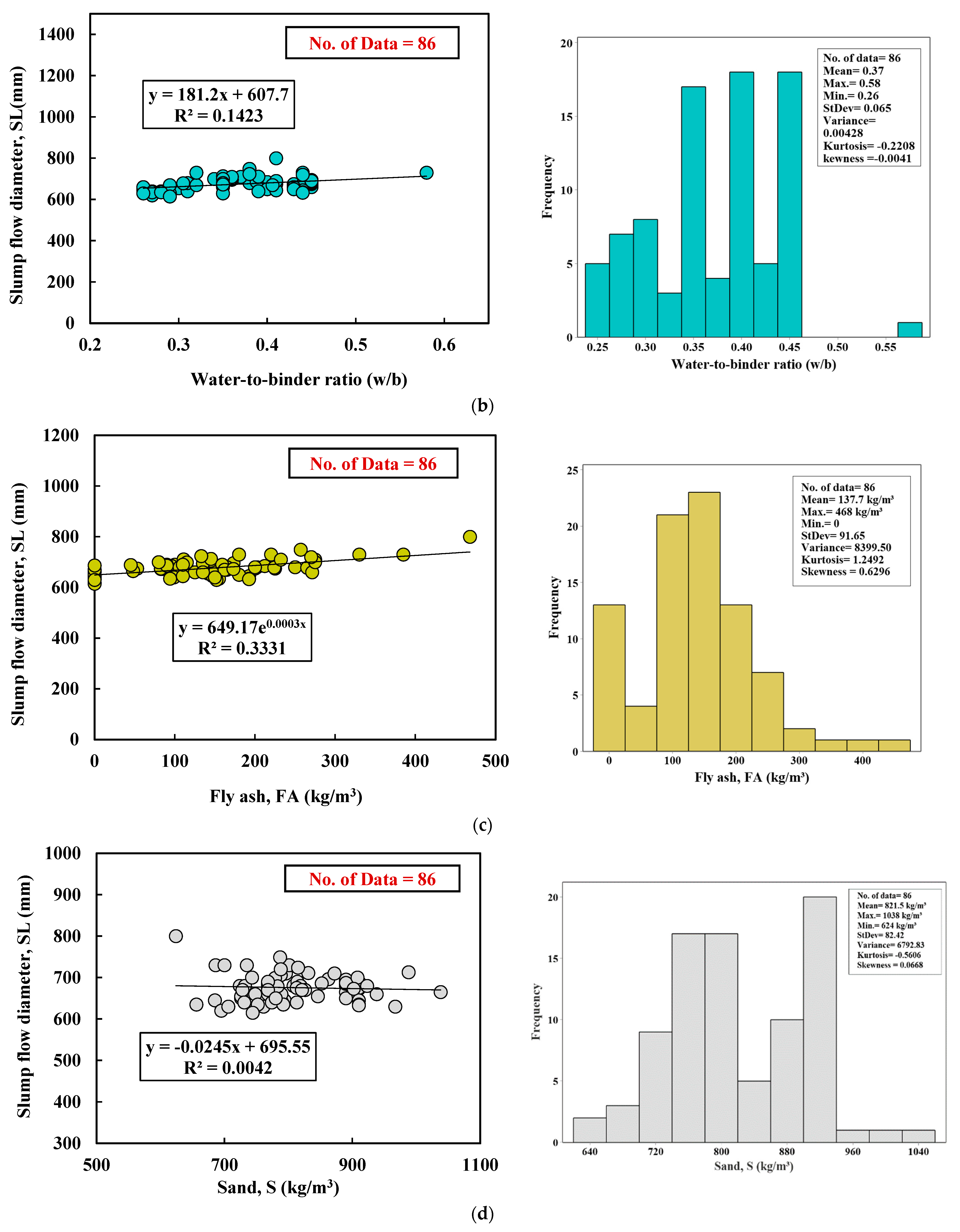
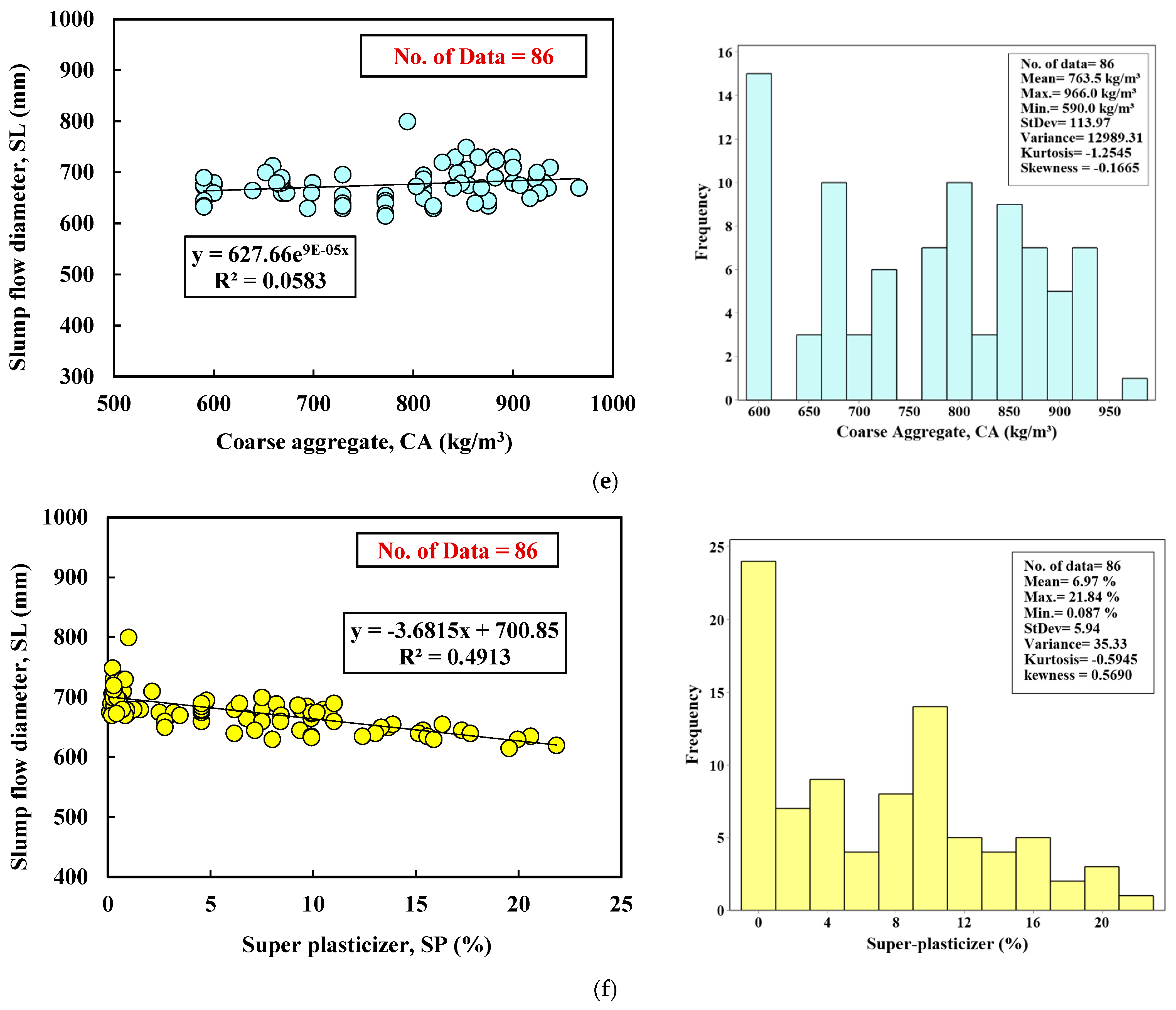
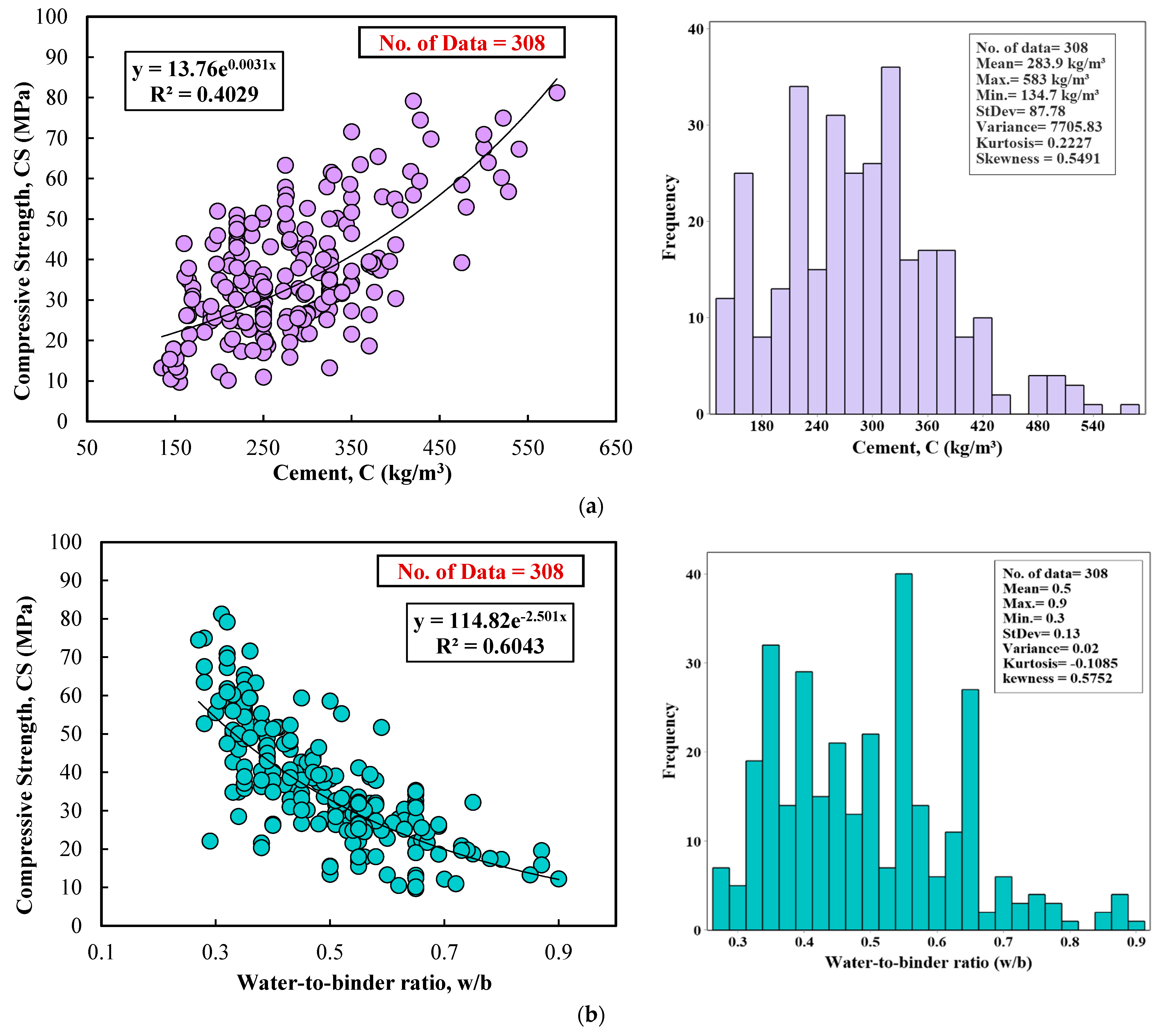
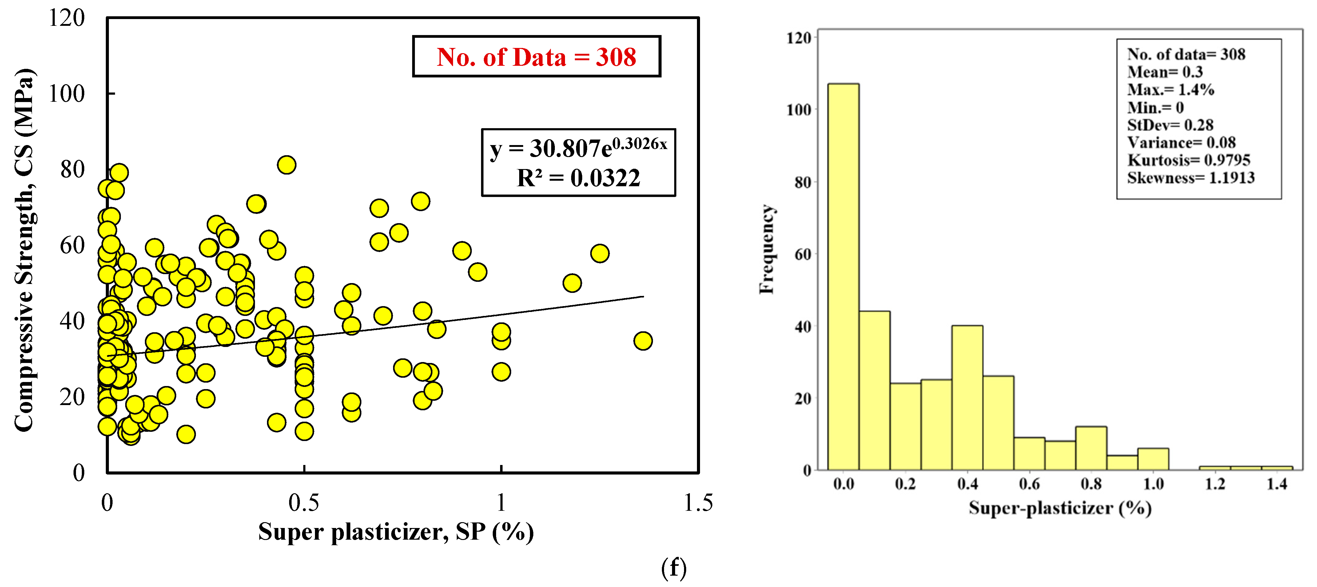
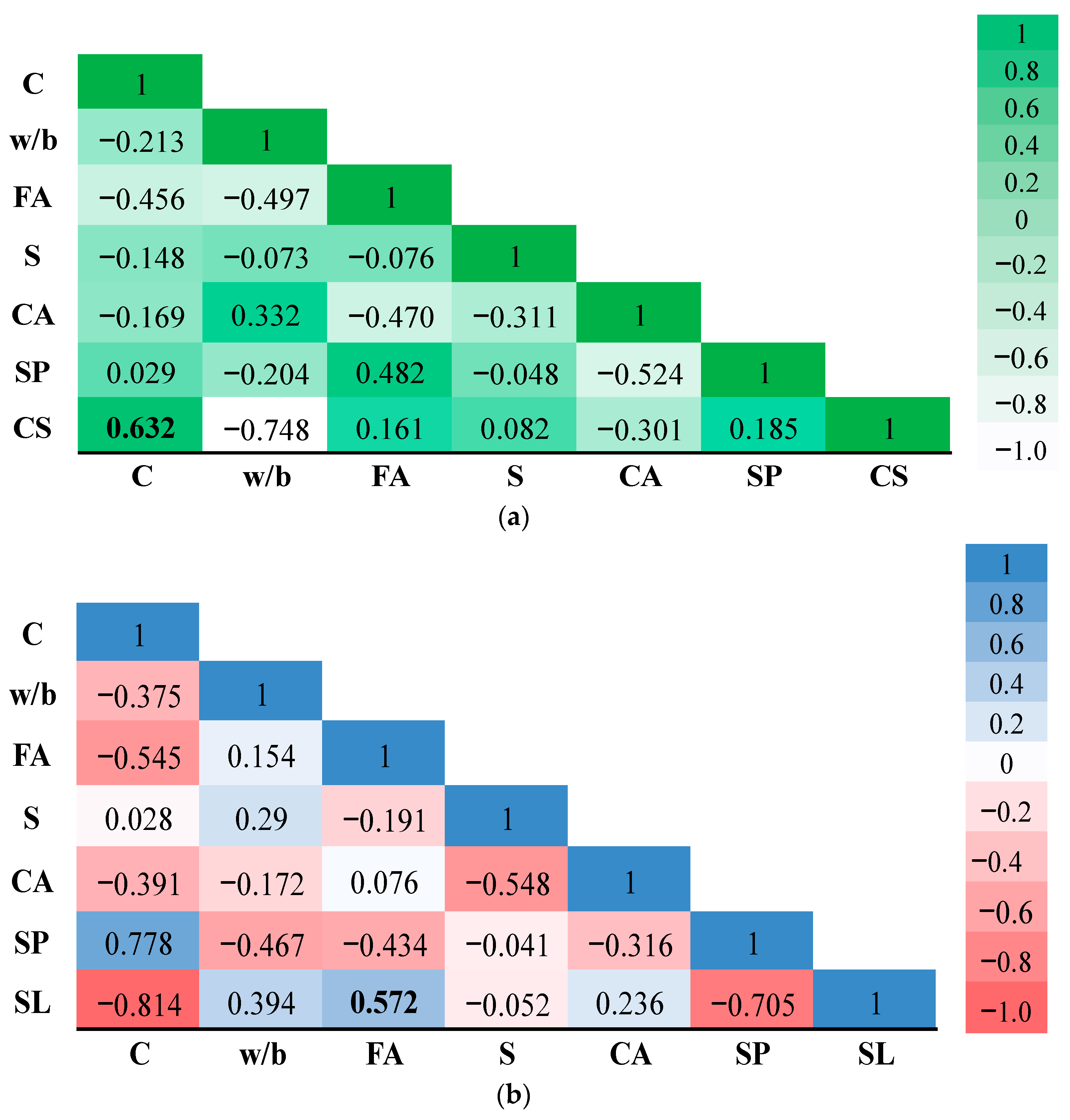
- Perform statistical analysis to determine the influence of concrete ingredients, such as the cement, water-to-binder ratio, fly ash, sand, coarse aggregate, and superplasticizer, on self-compacted concrete’s compressive strength and slump flow diameter.
- II.
- Provide a systematic multiscale model and propose to predict the compressive strength and slump flow diameter of self-compacted concrete containing up to 70% of fly ash, with a variety of cement, sand, and coarse aggregate content, as well as different water-to-binder ratios and superplasticizer percentages.
- III.
- Apply the most accurately developed model on different compressive strength ranges and slump flow diameter classes.
- IV.
- As an alternative to the developed model techniques (NLR, MLR, and ANN), determine the most reliable and accurate model based on different statistical assessment criteria to predict the CS and SL of fly ash-based self-compacted concrete.
- V.
- The overall and main objective of the current study is to model compressive strength as one of the significant mechanical properties of concrete and slump flow diameter as a fresh state property of SCC modified with different FA content.
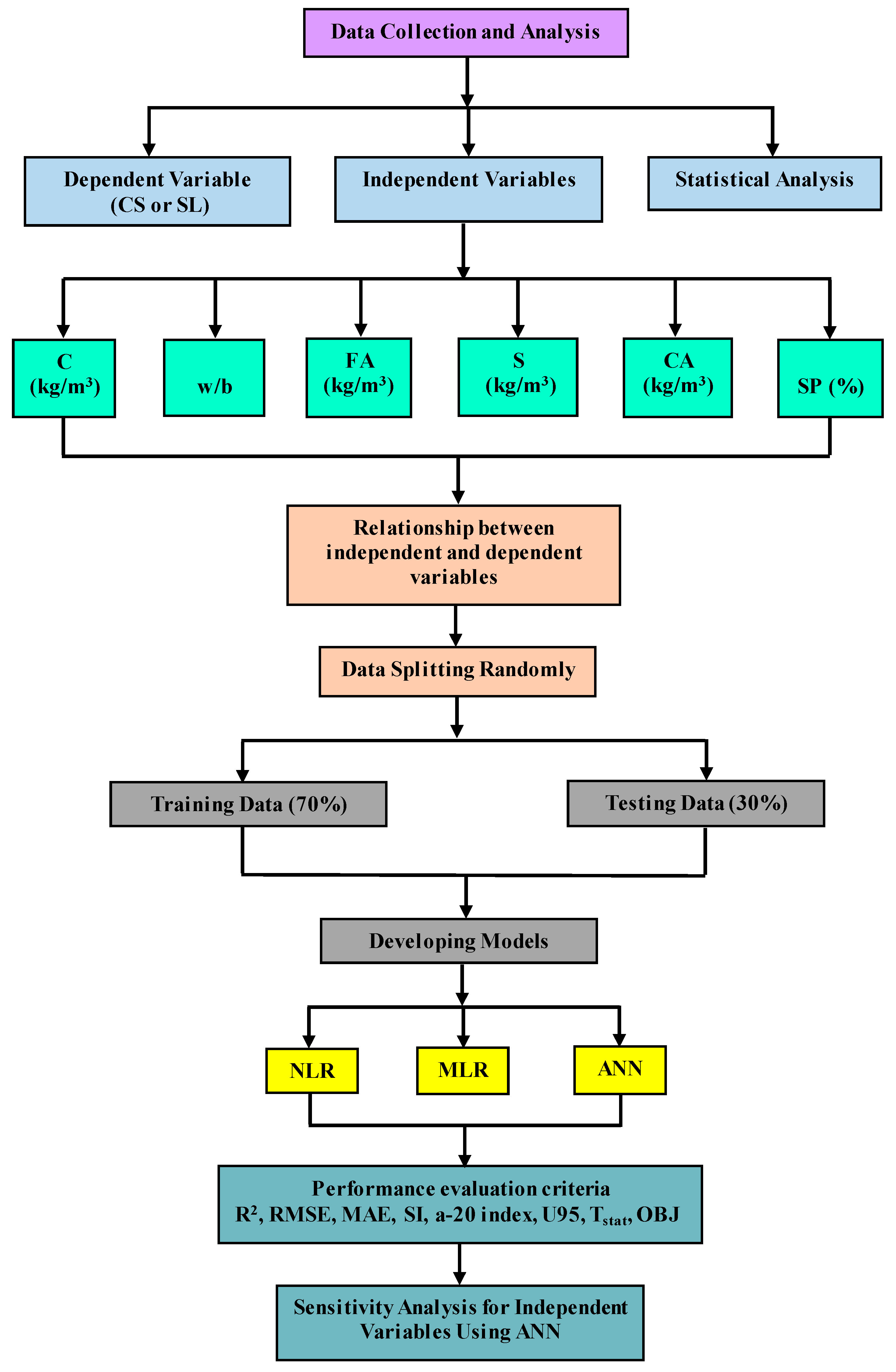
2. Methodology
2.1. Data Collection

| References | Cement, C (kg/m³) | Water-to-Binder Ratio (w/b) | Fly Ash, FA (kg/m³) | Sand, S (kg/m³) | Coarse Aggregate, CA (kg/m³) | Superplasticizer, SP (%) | Compressive Strength, CS (MPa) |
|---|---|---|---|---|---|---|---|
| [30] | 134.7–540 | 0.27–0.9 | 0–525 | 487–1135 | 600–1125 | 0–1.36 | 9.74–79.19 |
| [31] | 160–280 | 0.34–0.45 | 120–240 | 808–1034 | 900 | 0.1–0.6 | 31–52 |
| [32] | 280–400 | 0.55–0.87 | 0–120 | 718–1042 | 850 | 0.12–0.75 | 13.3–41.2 |
| [33,34] | 183–317 | 0.38–0.65 | 100–261 | 478–919 | 837 | 0–1 | Oct-43 |
| [35] | 533–583 | 0.31–0.33 | 50–215 | 813–835 | 745–766 | 0.24–0.46 | 50–81 |
| [36] | 161–247 | 0.35–0.45 | 159–254 | 842–866 | 843–864 | 0–0.4 | 26.2–38.0 |
| [37] | 250–427 | 0.31–0.59 | 90–257 | 768–988 | 659–923 | 0.09–0.9 | 47–66 |
| [38] | 220–440 | 0.32 | 110–330 | 686–714 | 881–917 | 0.62–0.69 | 48–70 |
| [39] | 300–350 | 0.38–0.4 | 150–200 | 830–845 | 860–876 | 0.818–0.827 | 21.6–26.5 |
| [40] | 380 | 0.38 | 20 | 1180 | 578 | 0.398 | 40.4 |
| [41] | 275–350 | 0.34–0.36 | 150–325 | 611–707 | 777–901 | 0.795–1.25 | 50–72 |
| [42] | 165–275 | 0.37–0.58 | 275–385 | 735–796 | 865–937 | 0.836–0.74 | 37.92–63.32 |
| [43] | 215 | 0.38 | 215 | 925 | 905 | 0.15 | 20.4 |
| [44] | 290 | 0.38 | 290 | 975 | 650 | 0.45 | 37.97 |
| [45] | 300 | 0.28 | 300 | 787 | 720 | 0.33 | 52.7 |
| [46] | 420 | 0.33 | 80 | 785 | 860 | 0.3 | 56 |
| [47] | 350 | 0.35 | 150 | 900 | 600 | 1.0 | 37.18 |
| [48] | 360 | 0.28 | 240 | 853 | 698 | 0.3 | 63.5 |
| [49] | 344–399 | 0.35 | 100–147 | 814 | 881–882 | 0.116–0.146 | 48.75–55 |
| [50] | 225 | 0.35 | 275 | 908 | 652 | 0.70 | 41.42 |
| [51] | 480 | 0.38 | 96 | 819 | 699 | 0.94 | 53 |
| References | Cement, C (kg/m³) | Water-to-binder ratio (w/b) | Fly ash, FA (kg/m³) | Sand, S (kg/m³) | Coarse aggregate, CA (kg/m³) | Superplasticizer, SP (%) | Slump flow diameter, SL (mm) |
| [52] | 450–480 | 0.40–0.45 | 0–144 | 890 | 810 | 4.8–13.3 | 650–695 |
| [50] | 500 | 0.35 | 0–275 | 908–967 | 652–694 | 0.7–8 | 630–700 |
| [37] | 220–427 | 0.31–0.41 | 90–330 | 686–988 | 659–923 | 0.18–0.9 | 670–749 |
| [38] | 550 | 0.32–0.44 | 0–110 | 728–826 | 855–935 | 3.2–8.43 | 670–675 |
| [53] | 530 | 0.45 | 0–265 | 768 | 668 | 0.09–4.55 | 660–690 |
| [41] | 83–385 | 0.31–0.41 | 165–468 | 624–732 | 794–931 | 1–1.25 | 680–800 |
| [31] | 430–450 | 0.36–0.39 | 202.5–232.2 | 872–808 | 900 | 1.58–2.15 | 680–710 |
| [54] | 465–550 | 0.41–0.44 | 83–193 | 910 | 590 | 0.97–11 | 635–690 |
| [55] | 450–500 | 0.39–0.43 | 135–225 | 724–789 | 850–926 | 2.5–6.15 | 640–680 |
| [56] | 500 | 0.35 | 150–250 | 900 | 600 | 10.5–11 | 660–680 |
| [57] | 550 | 0.41–0.44 | 83–193 | 910 | 590 | 9.91–11.01 | 633–690 |
| [58] | 180–270 | 0.44 | 180–270 | 788–801 | 829–842 | 0.27–0.28 | 720–730 |
| [42] | 165–385 | 0.29–0.58 | 165–385 | 735–821 | 865–966 | 0.74–0.84 | 670–730 |
| [59] | 567–670 | 0.26–0.31 | 0–156 | 656–846 | 729–875 | 12.39–21.84 | 615–655 |
| [60] | 733 | 0.26 | 271.21 | 748 | 698 | 8.40 | 660 |
| [49] | 399 | 0.35 | 100 | 814 | 882 | 0.146 | 690 |
| [61] | 500 | 0.35 | 0 | 1038 | 639 | 6.75 | 665 |
| [51] | 480 | 0.38 | 96 | 819 | 699 | 0.94 | 680 |
| [62] | 437 | 0.34 | 80 | 743 | 924 | 0.43 | 700 |
| [63] | 321.75 | 0.36 | 173.25 | 862.45 | 729.18 | 0.545 | 696 |

2.2. Pre-Processing
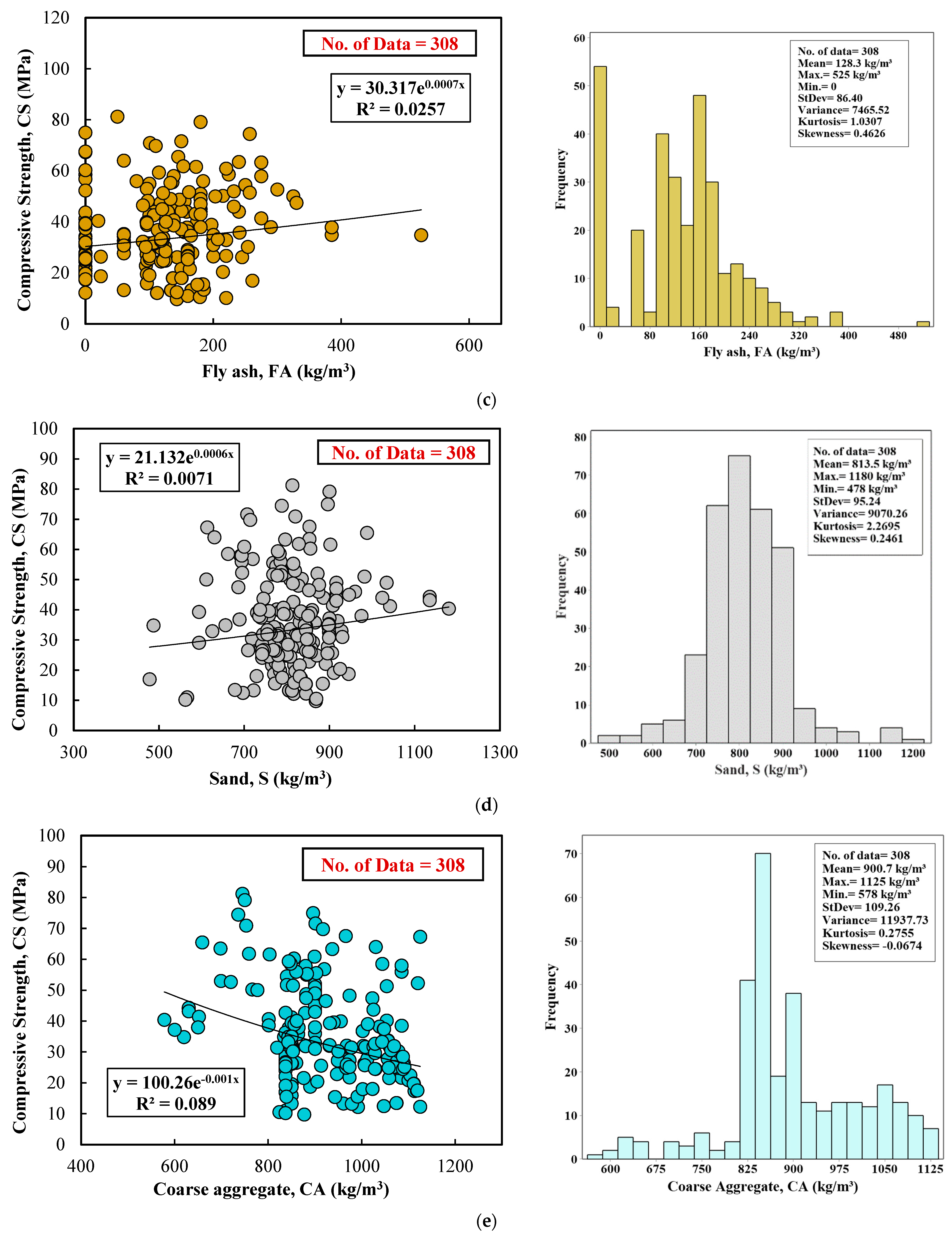
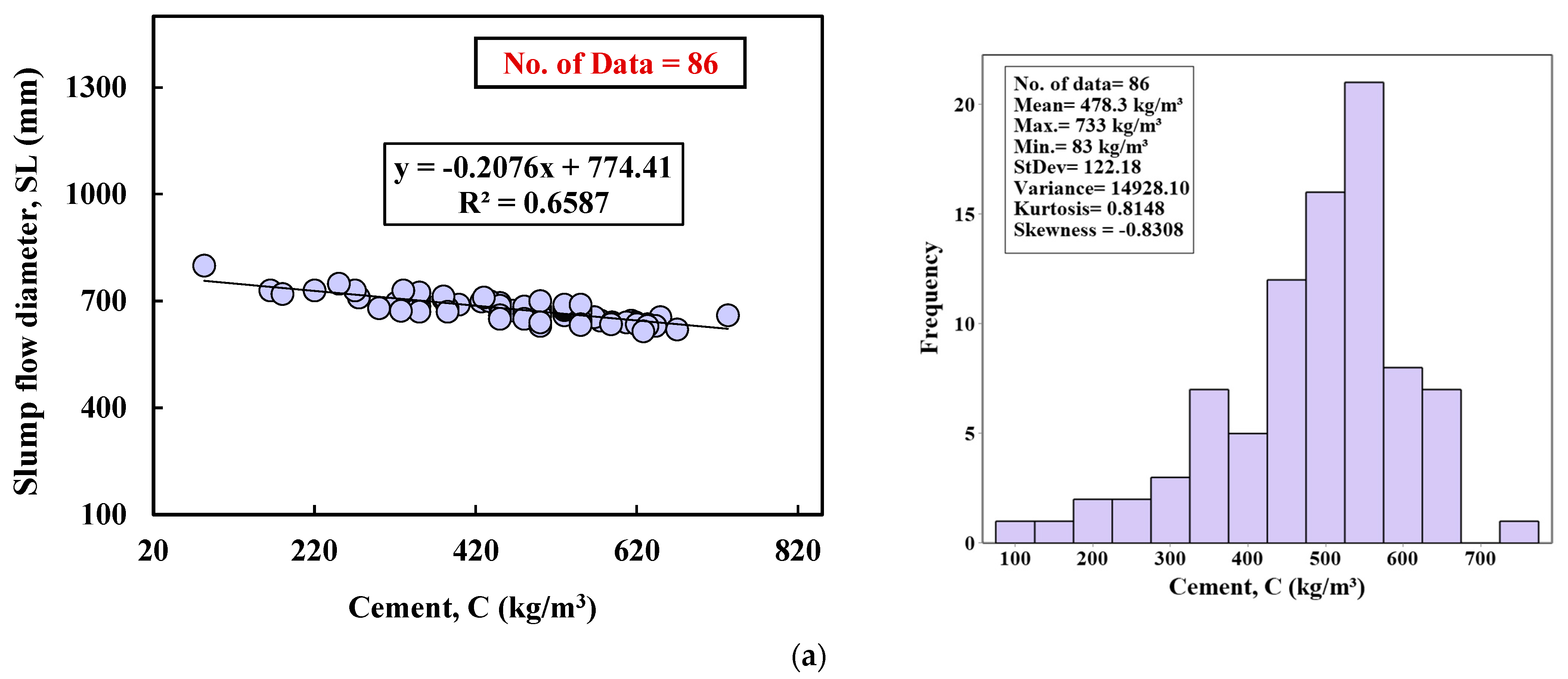
2.3. Statistical Evaluation
| Compressive strength database | Variables | C (kg/m³) | w/b | FA (kg/m3) | S (kg/m3) | CA (kg/m3) | SP (%) | CS (MPa) |
|---|---|---|---|---|---|---|---|---|
| Mean | 283.9 | 0.5 | 128.3 | 813.5 | 900.7 | 0.3 | 36.6 | |
| Median | 279.8 | 0.5 | 133 | 813.5 | 881 | 0.2 | 34.5 | |
| Mode | 250 | 0.55 | 0 | 916 | 837 | 0 | 49 | |
| SD | 87.78 | 0.13 | 86.4 | 95.24 | 109.26 | 0.28 | 15.08 | |
| Var | 7705.83 | 0.02 | 7465.52 | 9070.26 | 11,937.73 | 0.08 | 227.5 | |
| Kurt | 0.2227 | −0.1085 | 1.0307 | 2.2695 | 0.2755 | 0.9795 | −0.2692 | |
| Skew | 0.5491 | 0.5752 | 0.4626 | 0.2461 | −0.0674 | 1.1913 | 0.4736 | |
| Min | 134.7 | 0.27 | 0 | 478 | 578 | 0 | 9.7 | |
| Max | 583 | 0.9 | 525 | 1180 | 1125 | 1.4 | 81.3 | |
| Slump flow database | Variables | C (kg/m³) | w/b | FA (kg/m3) | S (kg/m3) | CA (kg/m3) | SP (%) | SL (mm) |
| Mean | 478.3 | 0.37 | 137.7 | 821.5 | 763.5 | 6.97 | 674.9 | |
| Median | 500 | 0.38 | 142.9 | 810.5 | 772 | 6.58 | 675 | |
| Mode | 550 | 0.35 | 0 | 910 | 590 | 4.55 | 680 | |
| SD | 122.18 | 0.065 | 91.65 | 82.42 | 113.97 | 5.94 | 31.52 | |
| Var | 14,928.1 | 0.00428 | 8399.5 | 6792.83 | 12,989.31 | 35.33 | 993.62 | |
| Kurt | 0.8148 | −0.2208 | 1.2492 | −0.5606 | −1.2545 | −0.5945 | 1.9597 | |
| Skew | −0.8308 | −0.0041 | 0.6296 | 0.0668 | −0.1665 | 0.569 | 0.8086 | |
| Min | 83 | 0.26 | 0 | 624 | 590 | 0.087 | 615 | |
| Max | 733 | 0.58 | 468 | 1038 | 966 | 21.84 | 800 |


2.4. Modeling
2.4.1. Nonlinear Regression (NLR) Model
2.4.2. Multi-Linear Regression (MLR) Model
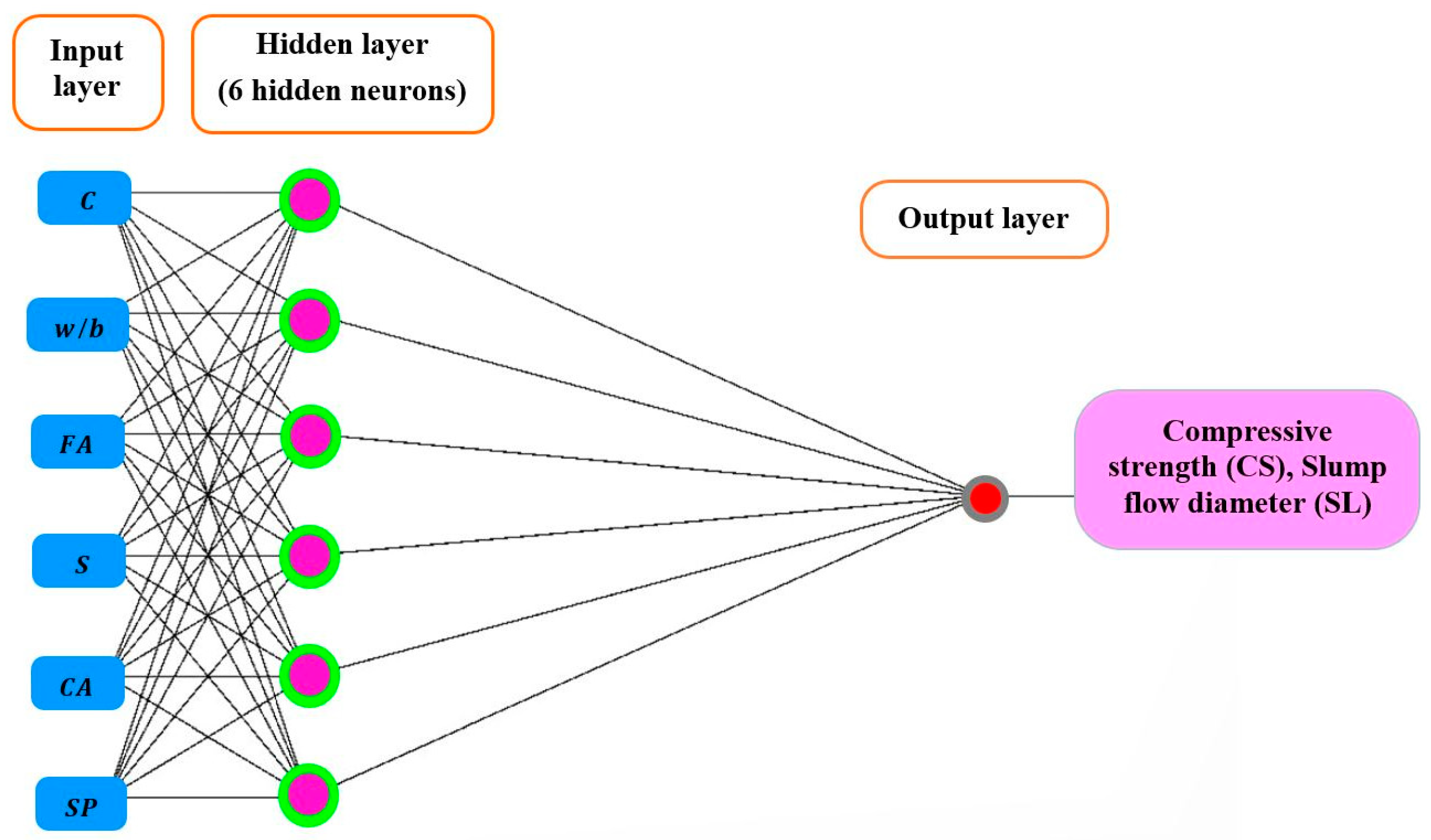
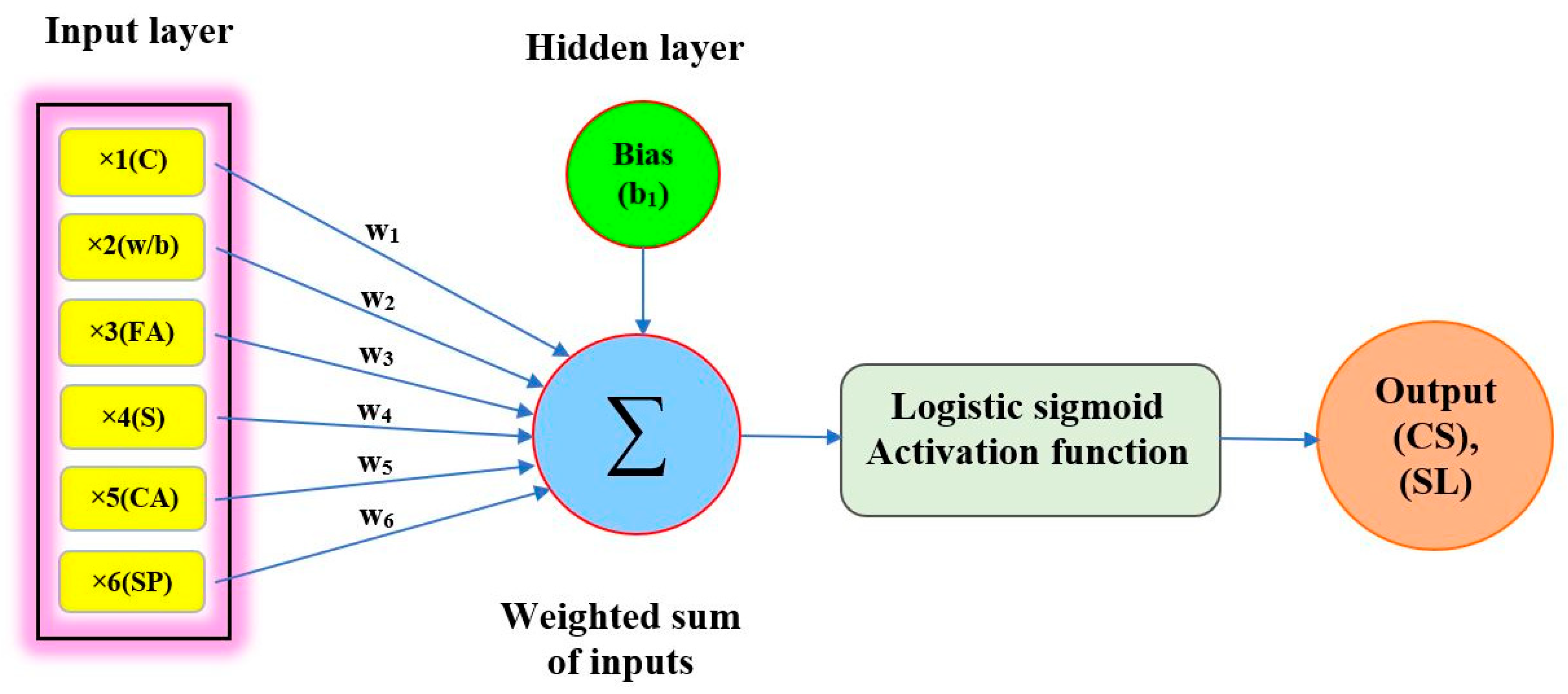
2.4.3. Artificial Neural Network (ANN) Model
2.5. Metrics for Assessing Developed Models
3. Results and Discussion
3.1. Relation between Predicted and Experimental Values
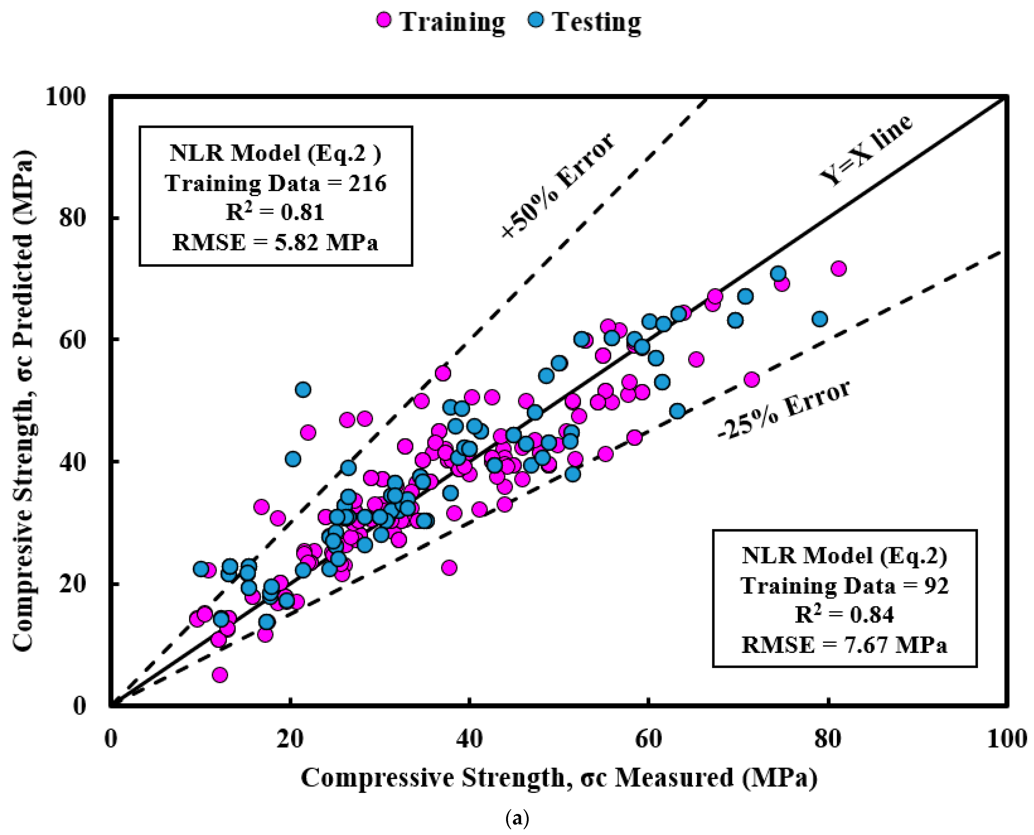
3.1.1. Nonlinear Regression (NLR) Model

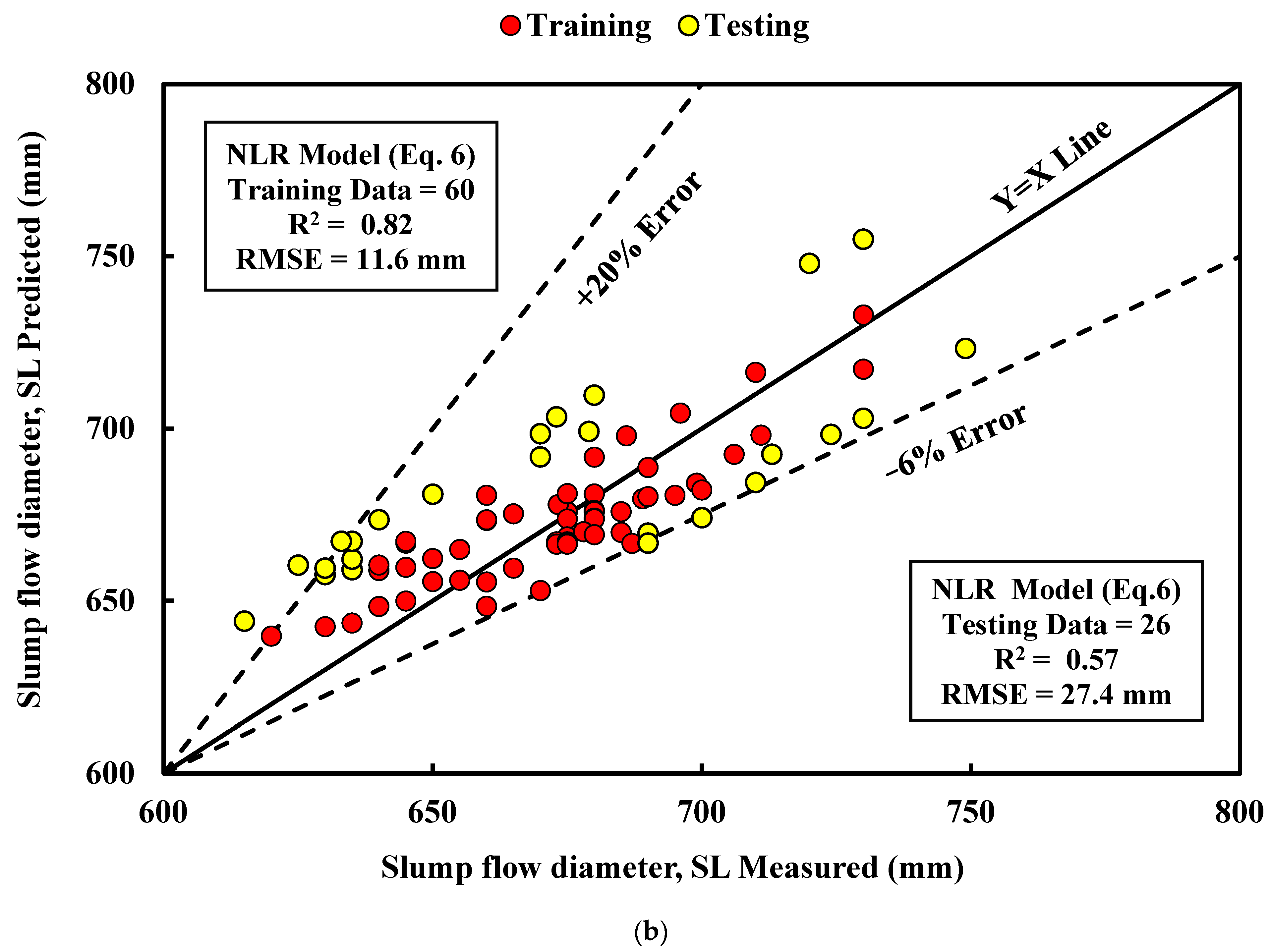
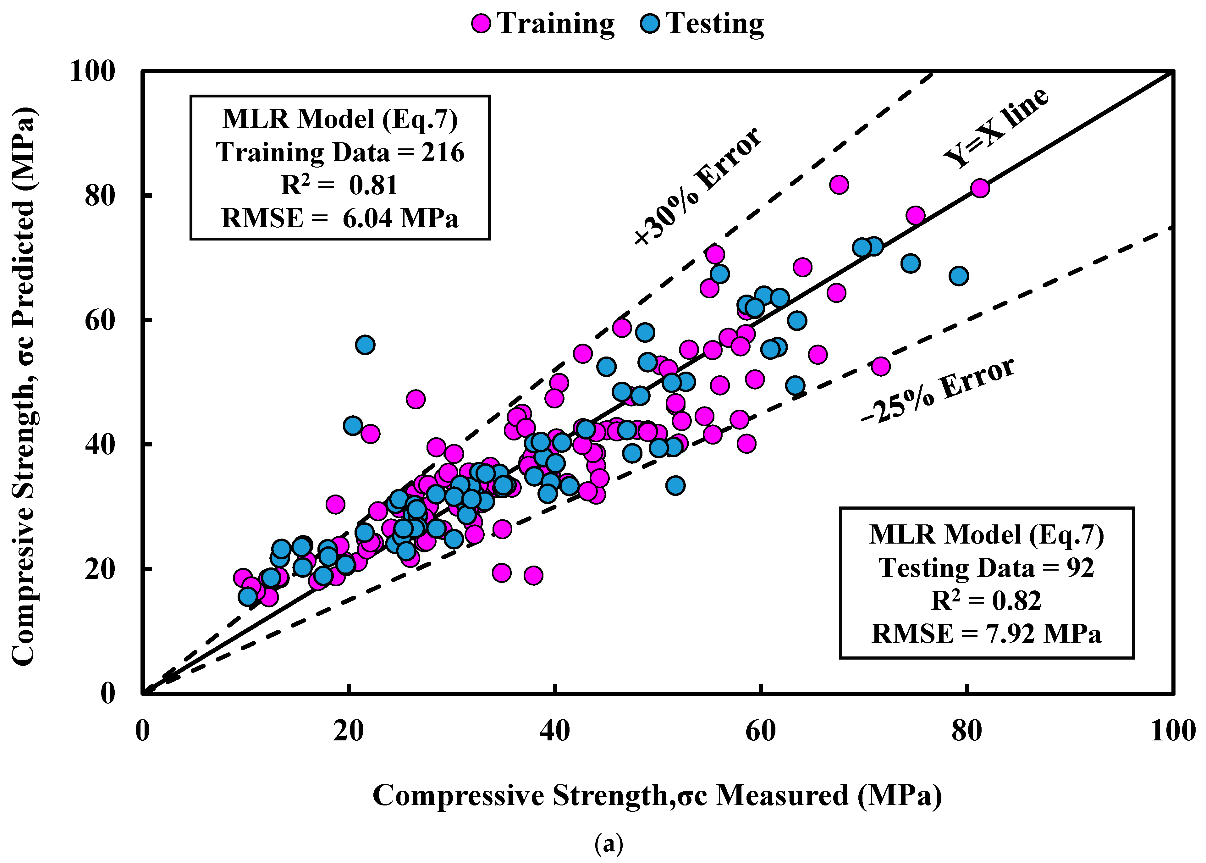
3.1.2. Multi-Linear Regression (MLR) Model


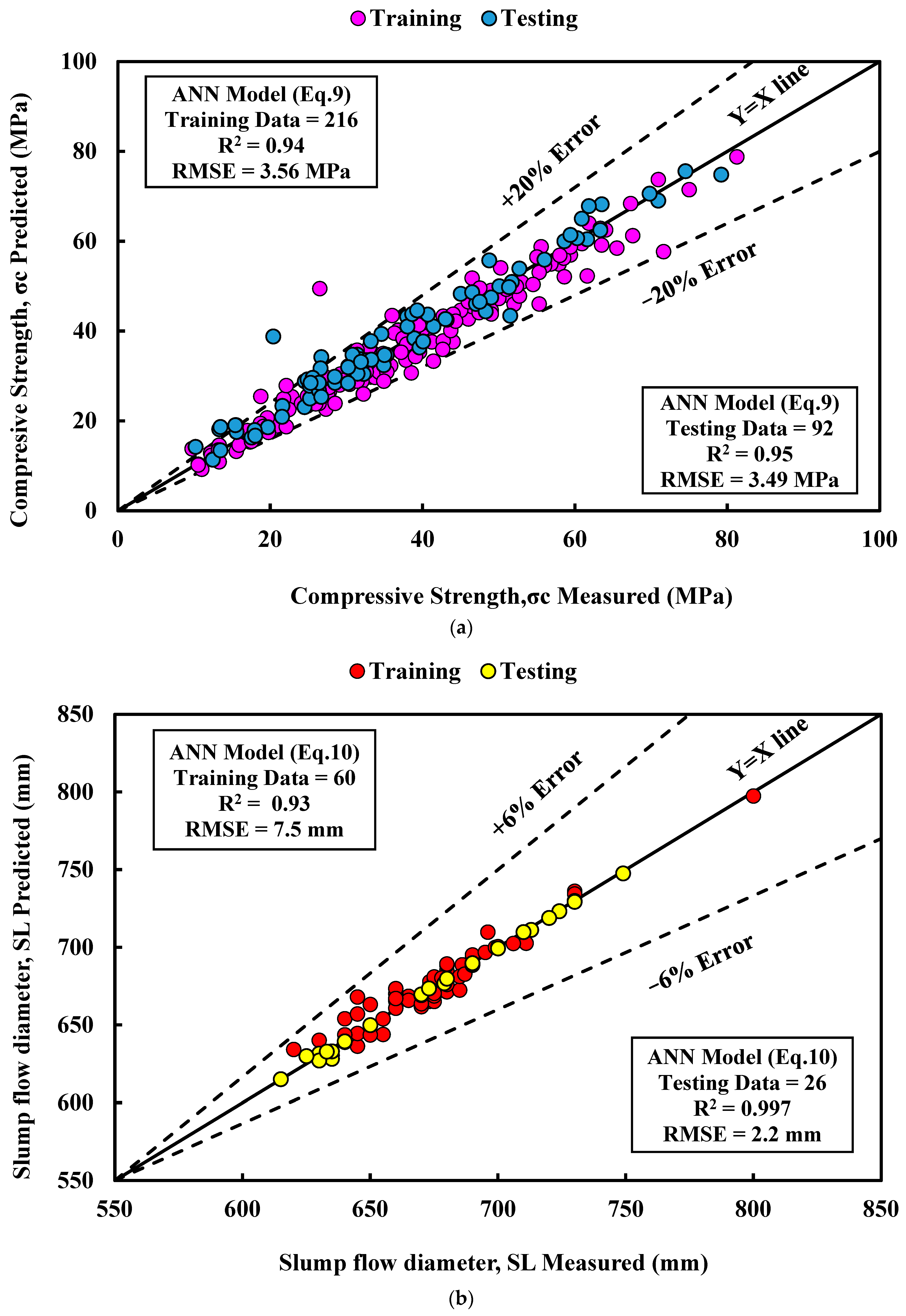
3.1.3. Artificial Neural Network (ANN) Model

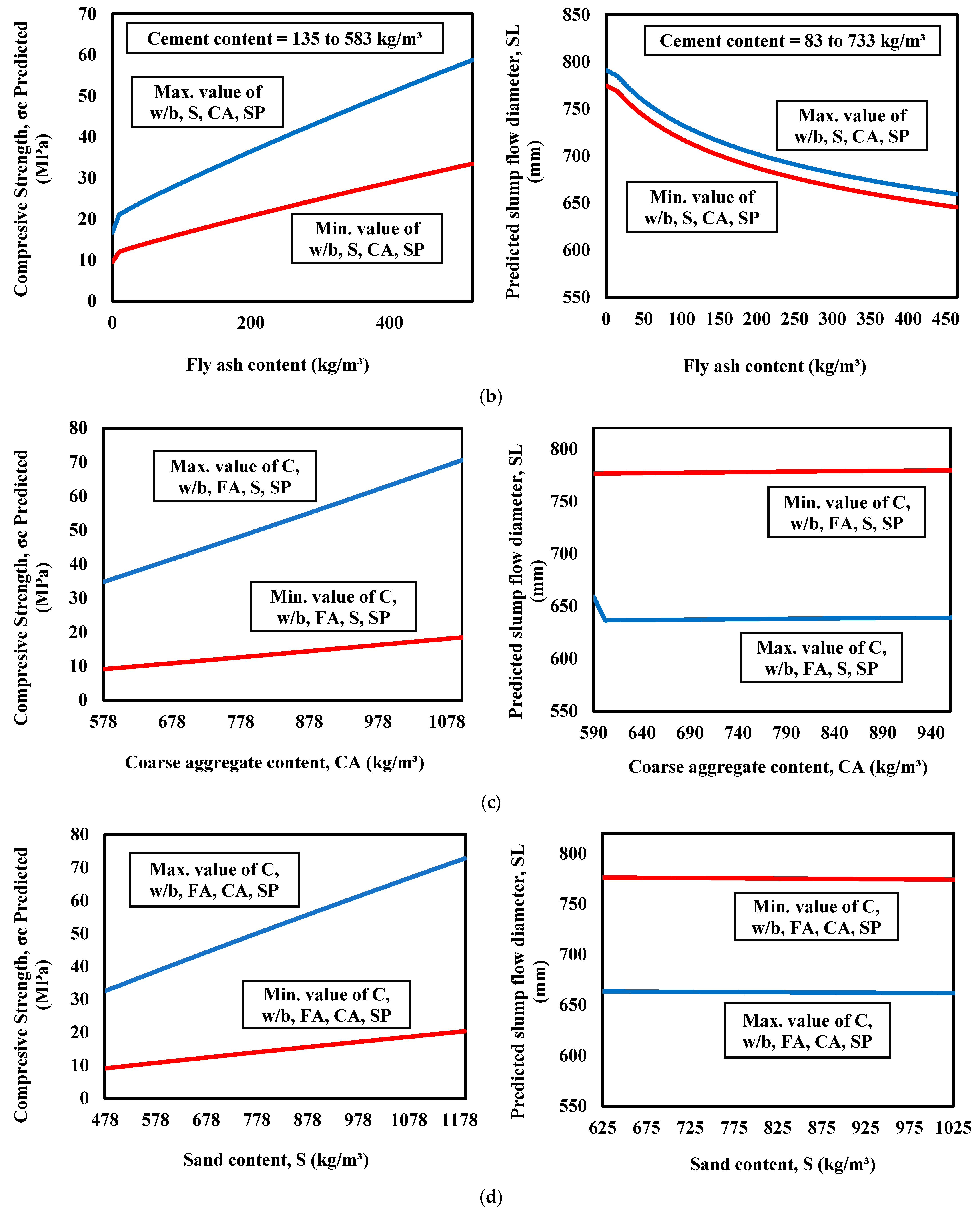
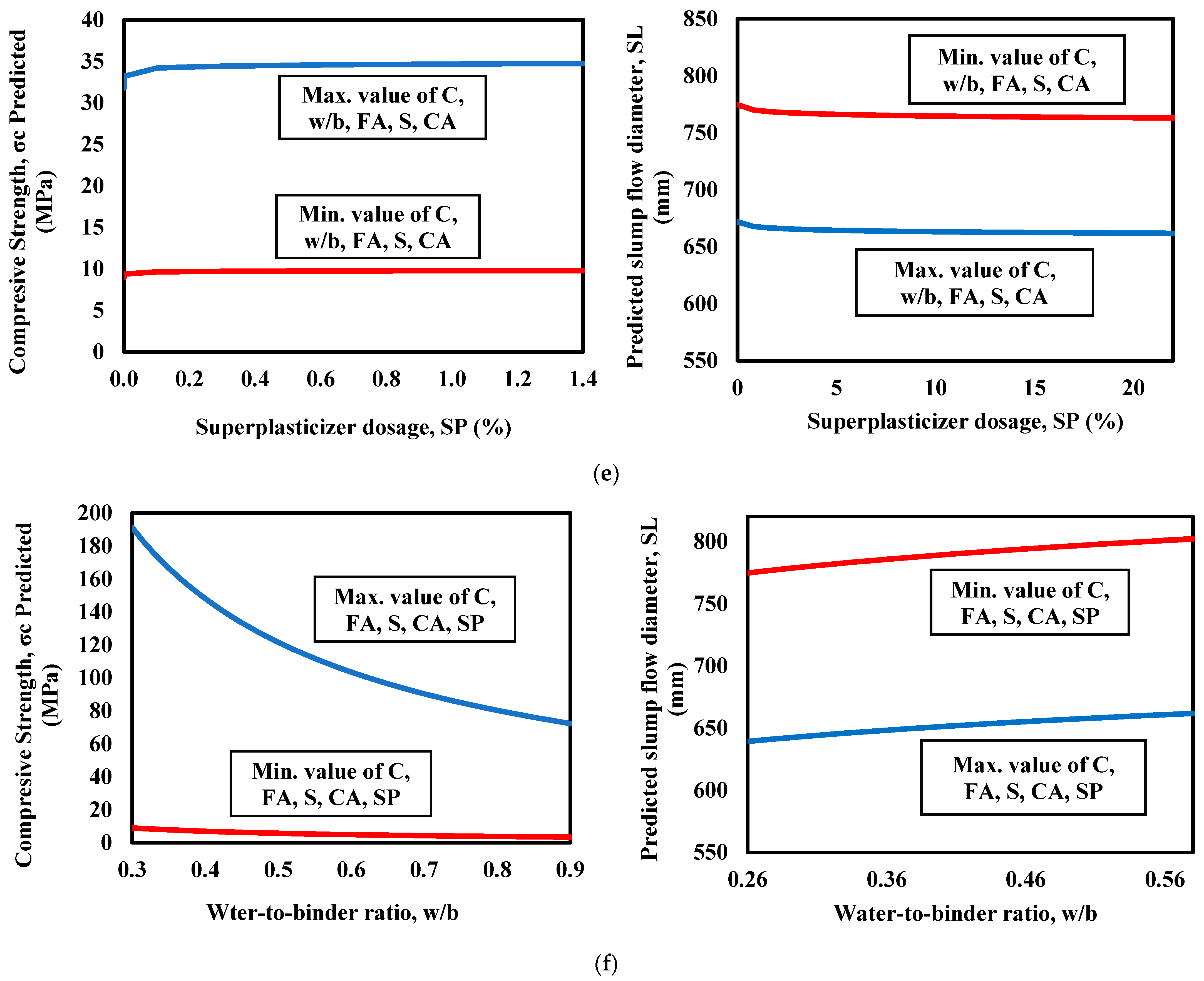
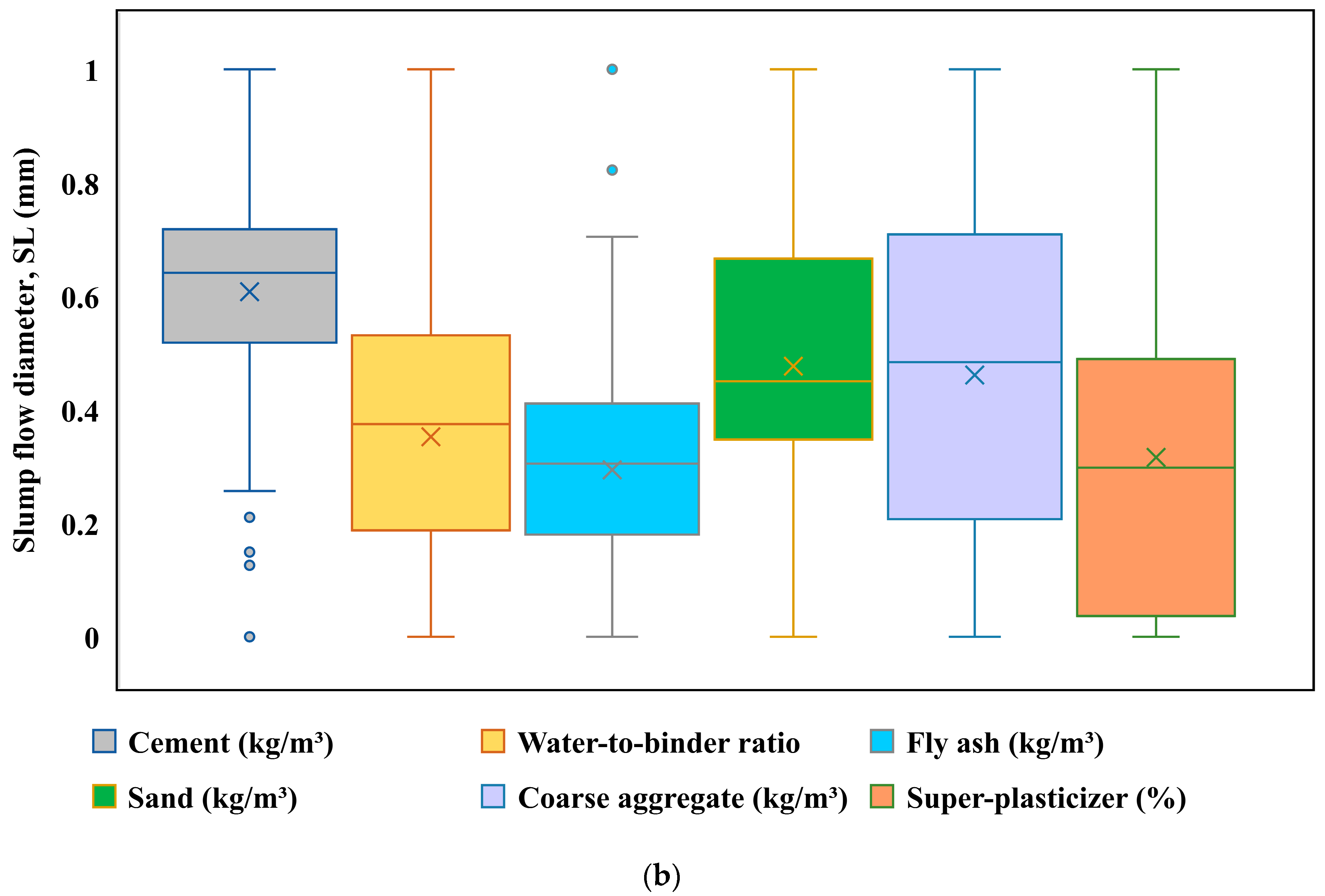
3.2. Effective Factors
4. Evaluation of Developed Models
5. Sensitivity Investigation

| Compressive strength | No. | Combination | Removed Parameter | R2 | RMSE (MPa) | MAE (MPa) | Ranking Based on RMSE and MAE |
|---|---|---|---|---|---|---|---|
| 1 | C, w/b, FA, S, CA, SP | - | 0.94 | 3.65 | 2.52 | - | |
| 2 | w/b, FA, S, CA, SP | C | 0.82 | 6.19 | 4.7 | 1 | |
| 3 | C, FA, S, CA, SP | w/b | 0.93 | 3.85 | 2.79 | 5 | |
| 4 | C, w/b, S, CA, SP | FA | 0.9 | 4.92 | 3.7 | 3 | |
| 5 | C, w/b, FA, CA, SP | S | 0.91 | 4.75 | 3.5 | 4 | |
| 6 | C, w/b, FA, S, SP | CA | 0.89 | 5.46 | 4.19 | 2 | |
| 7 | C, w/b, FA, S, CA | SP | 0.94 | 3.83 | 2.6 | 6 | |
| Slump flow diameter | No. | Combination | Removed Parameter | R2 | RMSE (mm) | MAE (mm) | Ranking based on RMSE and MAE |
| 1 | C, w/b, FA, S, CA, SP | - | 0.93 | 7.5 | 6 | - | |
| 2 | w/b, FA, S, CA, SP | C | 0.87 | 10.9 | 9.2 | 1 | |
| 3 | C, FA, S, CA, SP | w/b | 0.91 | 8.7 | 6.5 | 6 | |
| 4 | C, w/b, S, CA, SP | FA | 0.88 | 9.5 | 7.8 | 3 | |
| 5 | C, w/b, FA, CA, SP | S | 0.9 | 9 | 7.2 | 5 | |
| 6 | C, w/b, FA, S, SP | CA | 0.88 | 9.5 | 7.9 | 2 | |
| 7 | C, w/b, FA, S, CA | SP | 0.9 | 9.4 | 7.6 | 4 |
6. Conclusions
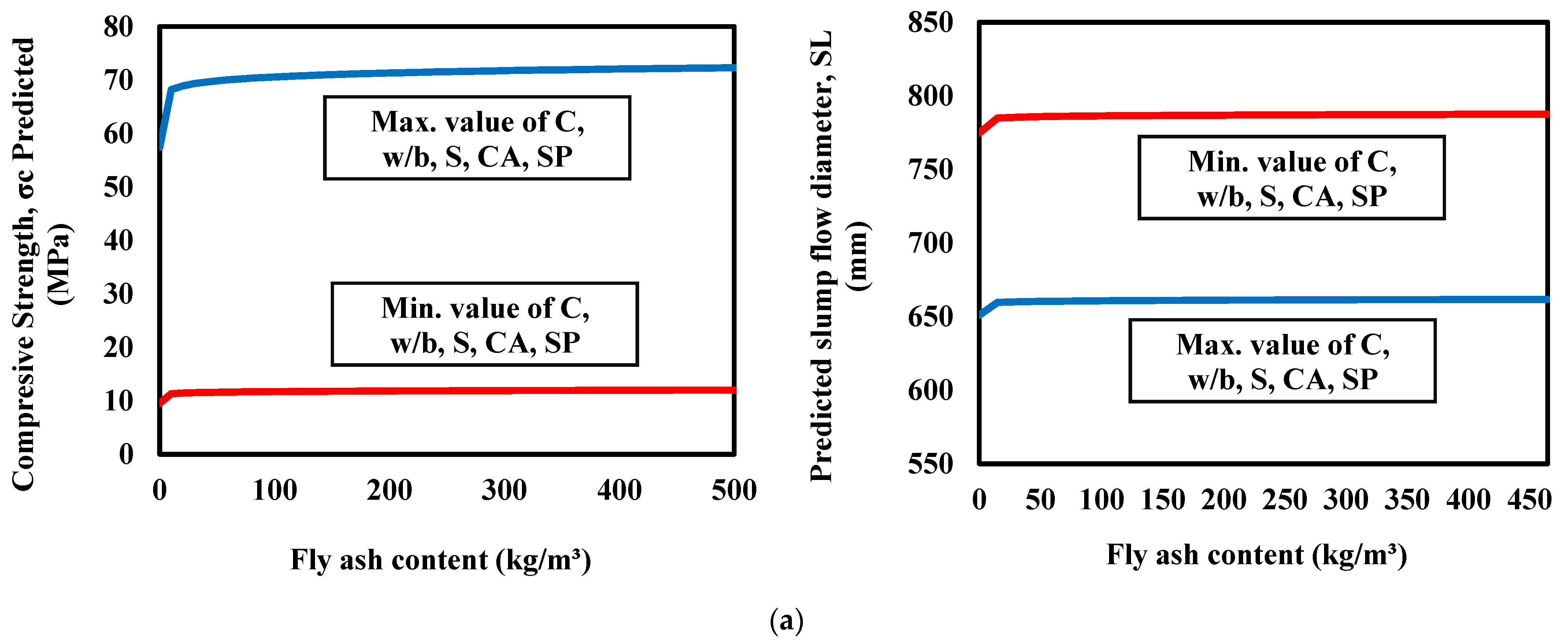
- The database for predicting CS included fly ash content ranging between 0 and 525 kg/m3, while that for predicting SL ranged between 0 and 468 kg/m3.
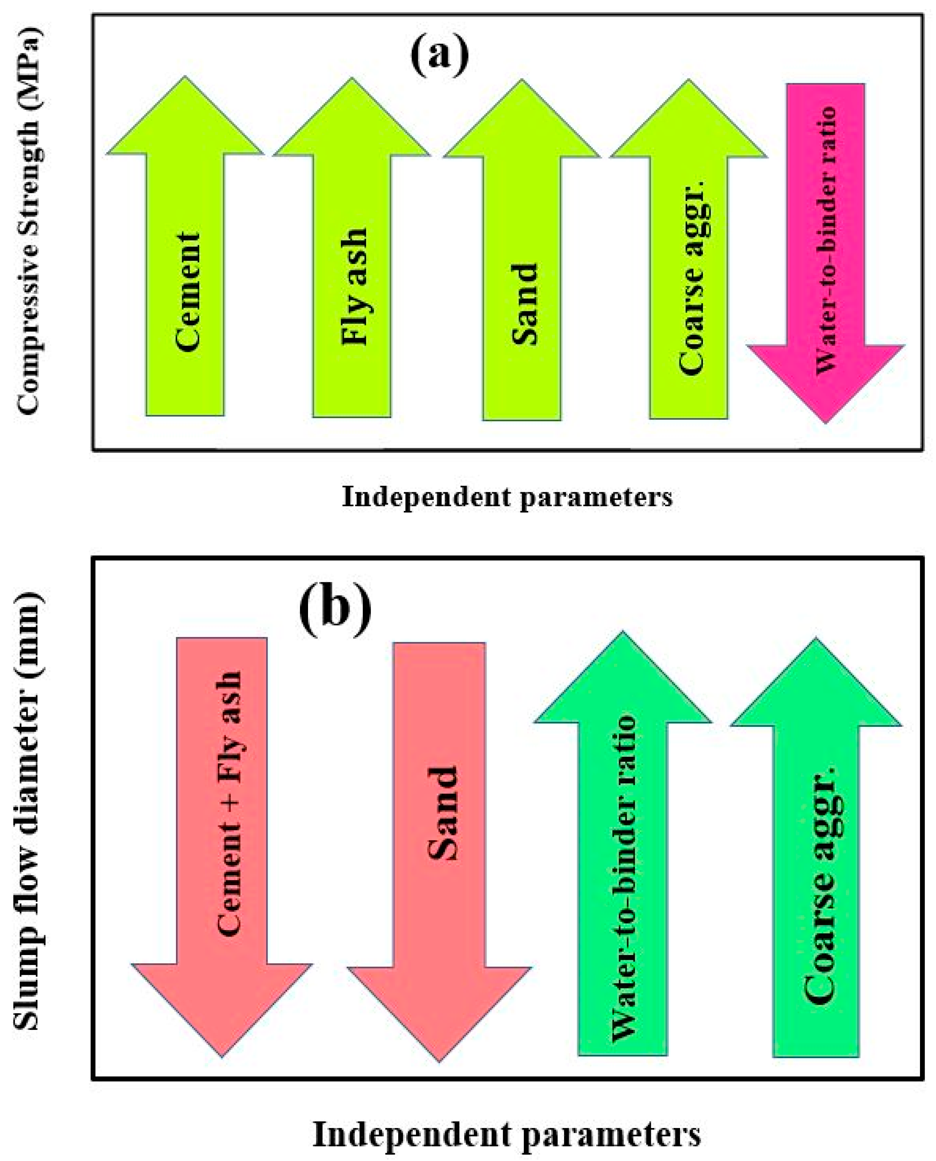
- Increasing fly ash content caused an increase in the CS, but a lower impact was found on the SL. However, the impact of fly ash was found when the cement content was increased with an increase in the fly ash content simultaneously. It decreased the SL but increased the CS.
- The compressive strength was more affected by aggregates rather than the slump flow. Increasing the CA and S content increased the CS but led to small changes in the SL. The influence of CA and S was noted to be higher at the maximum values of the variables. These findings highlight the importance of aggregates, specifically coarse and fine aggregates, in determining the compressive strength of concrete. Whereas the slump flow, which measures the workability and fluidity of the mixture, did not substantially impact the CS, the composition and content of aggregates played a crucial role in enhancing the concrete’s overall strength.
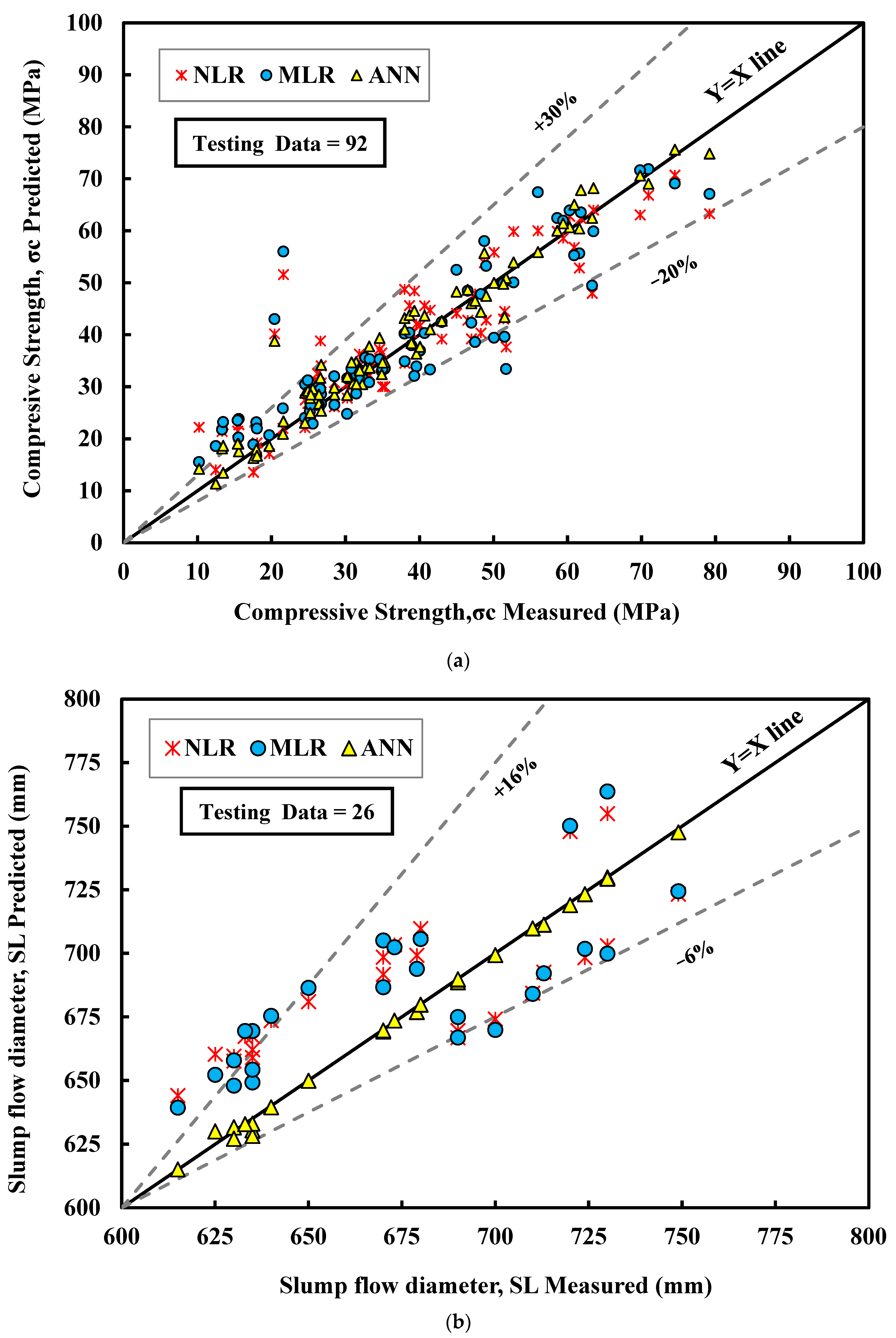
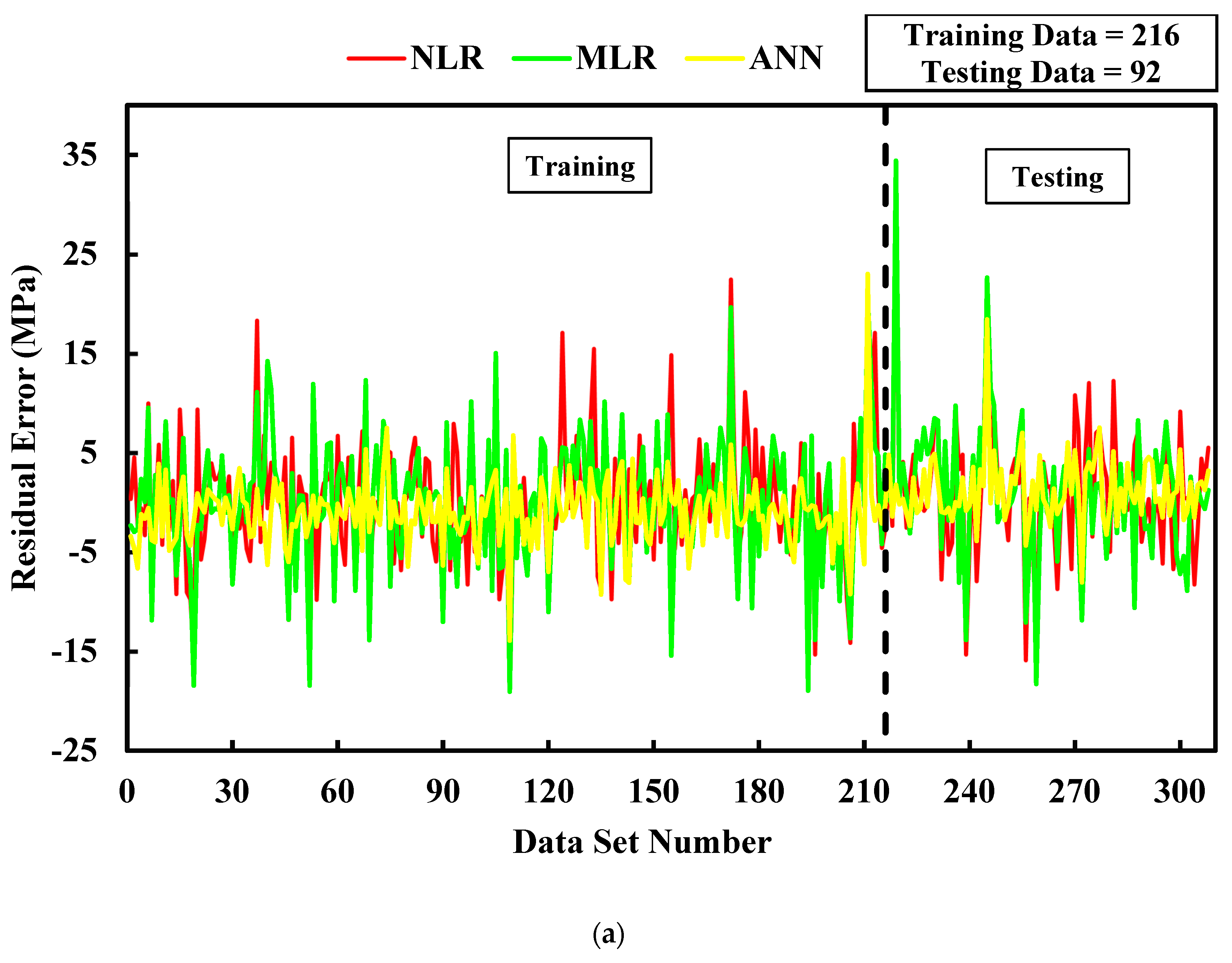
- According to the various assessment criteria, such as R2, RMSE, and MAE, the ANN model was noted to have the highest accuracy and reliability for predicting both compressive strength and slump flow diameter of self-compacted concrete.
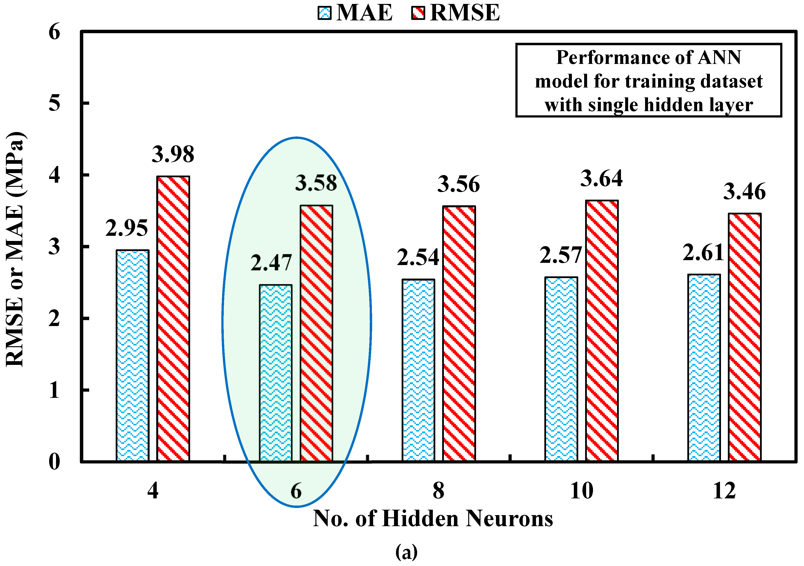
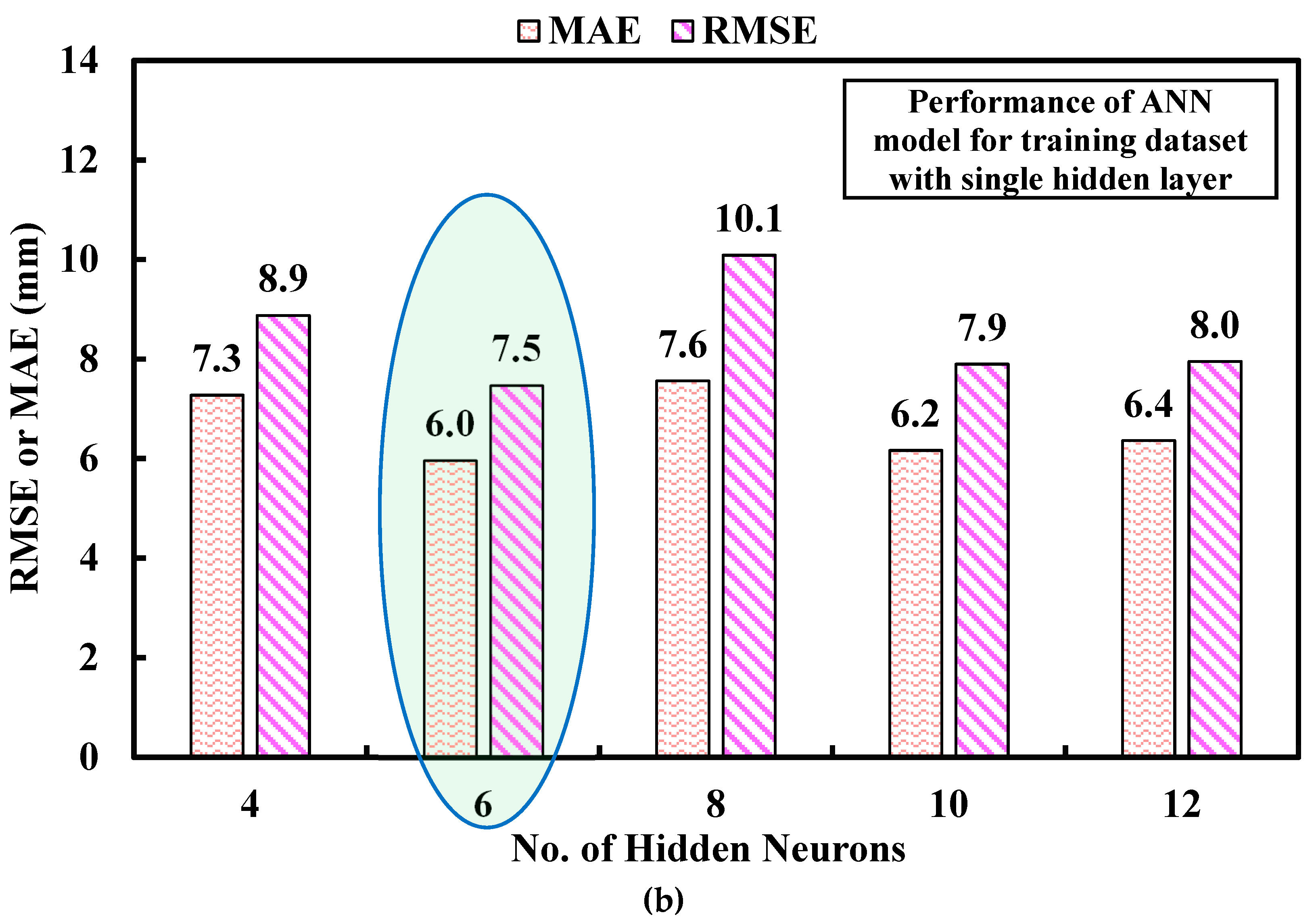
- When predicting the CS, the ANN model had the highest R2 of 0.94 for training and 0.95 for testing datasets. The lowest RMSE and MAE values were found to be 3.56 MPa and 2.54 MPa for training and 3.49 MPa and 2.45 MPa for testing datasets, respectively. However, in predicting the SL, the ANN model had an R2 value of 0.93, RMSE of 7.5 mm, and MAE of 5.97 mm for the training dataset. The testing dataset’s R2, RMSE, and MAE values were 0.997, 2.2 mm, and 1.39 mm, respectively.
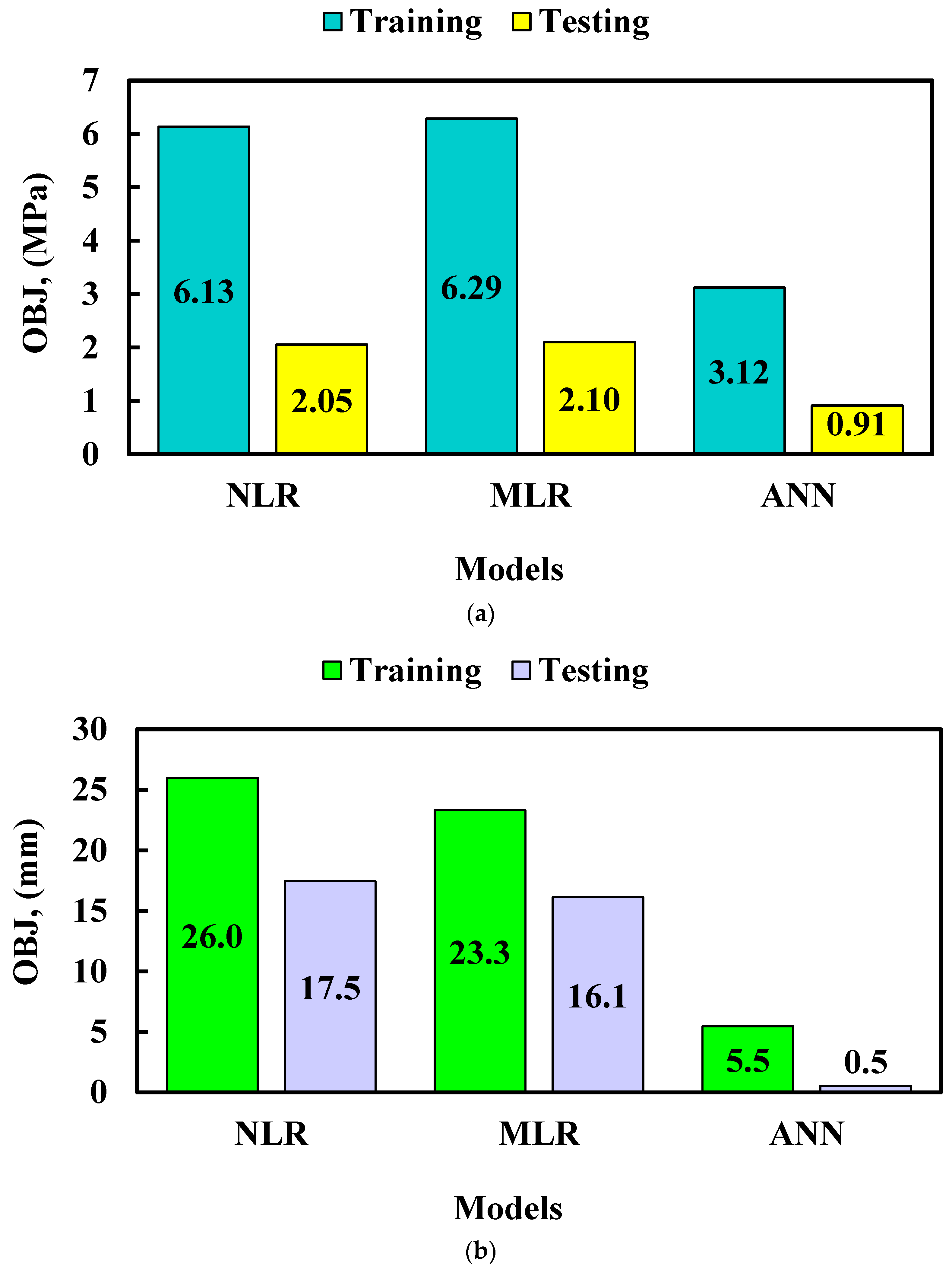
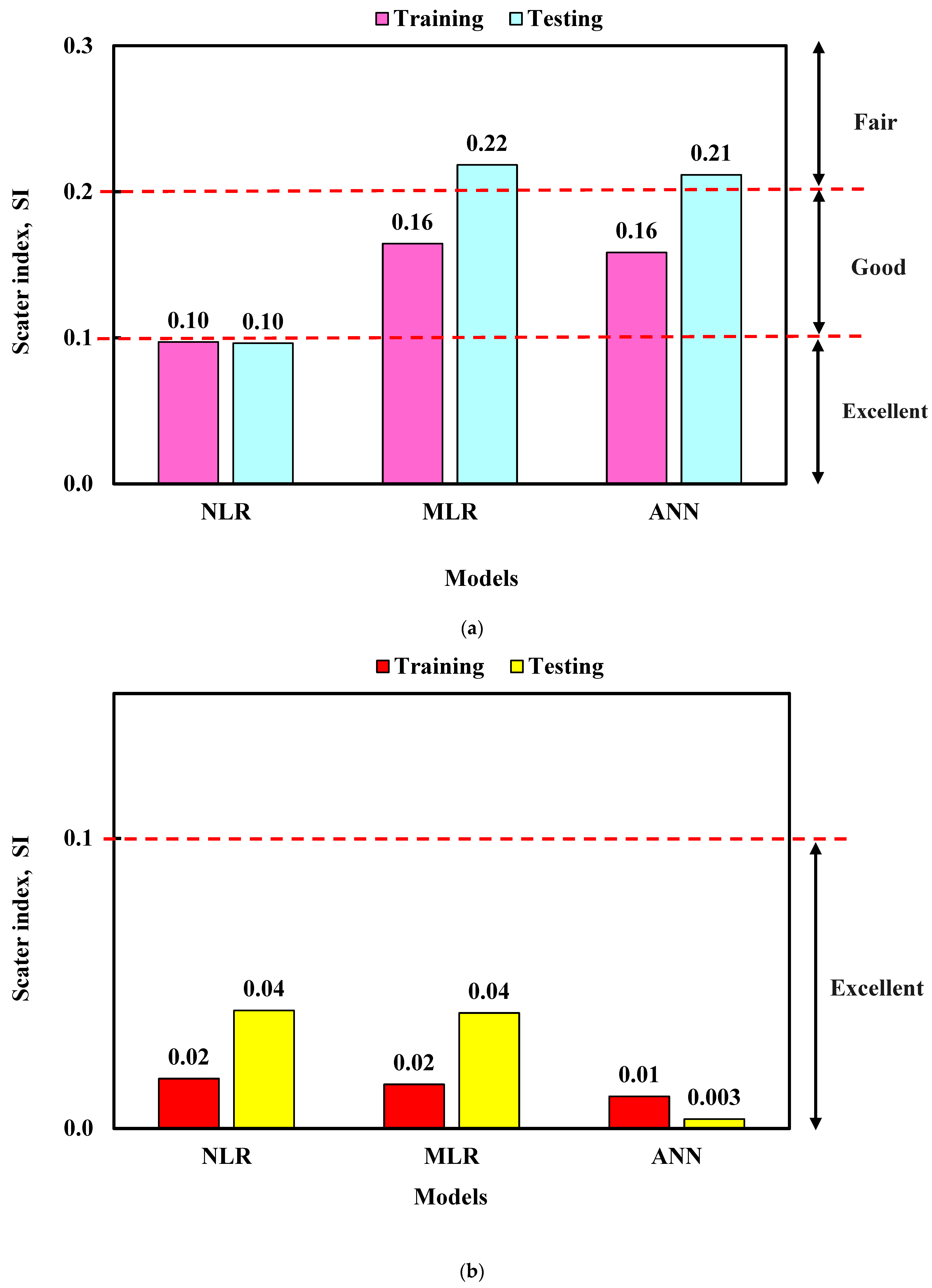
- Other statistical assessment tools, such as the OBJ function and SI value, were used. The ANN model maintained the lowest OBJ value of 3.12 and 5.5 for the CS and SL, respectively. Regarding the SI value, excellent performance was observed from the NLR model when predicting the CS, which was 0.10 for both the training and testing datasets. However, all models were observed to predict the SL. The SI value was 0.02 for both the NLR and MLR models and 0.01 for the ANN model.
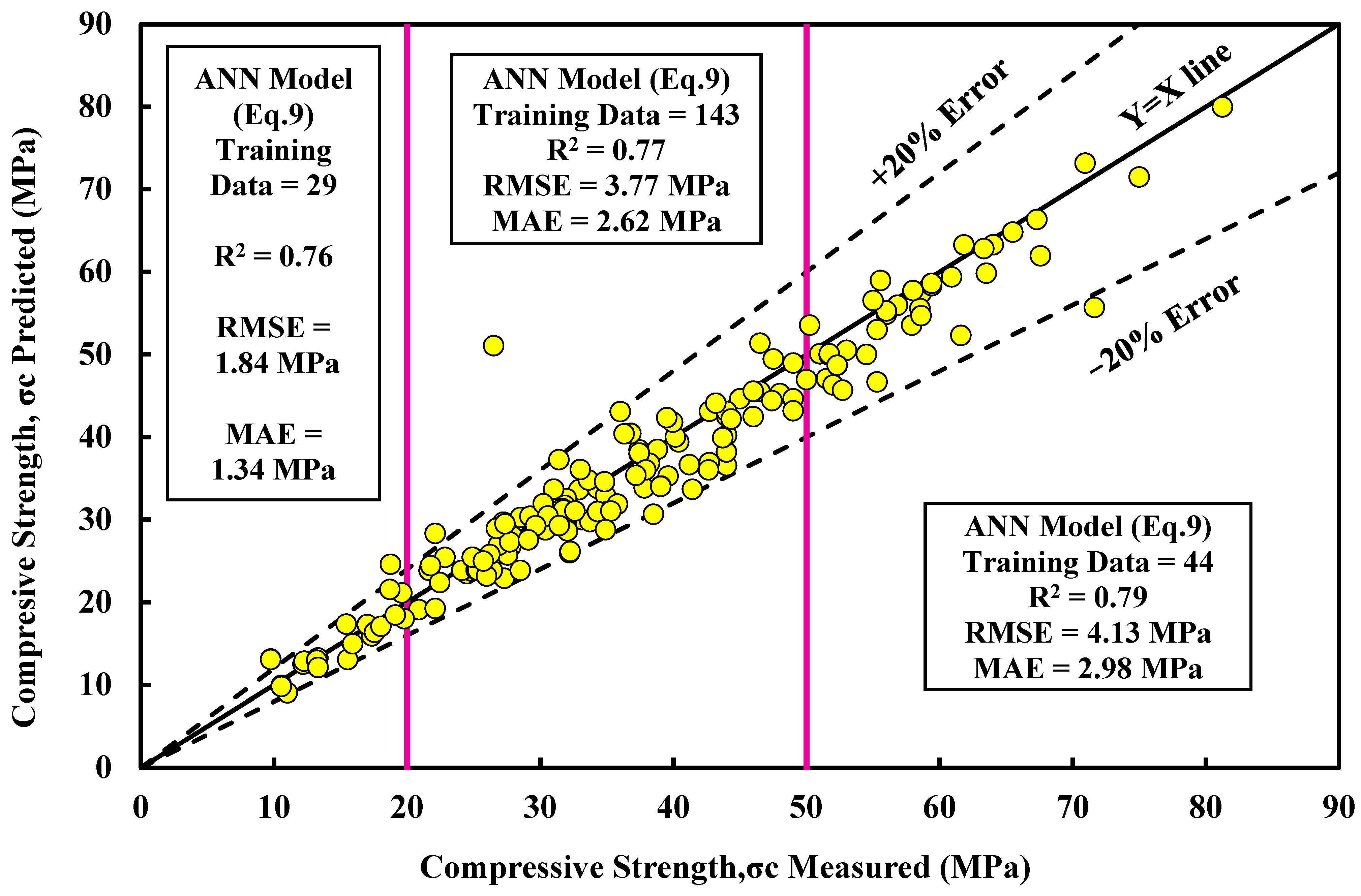
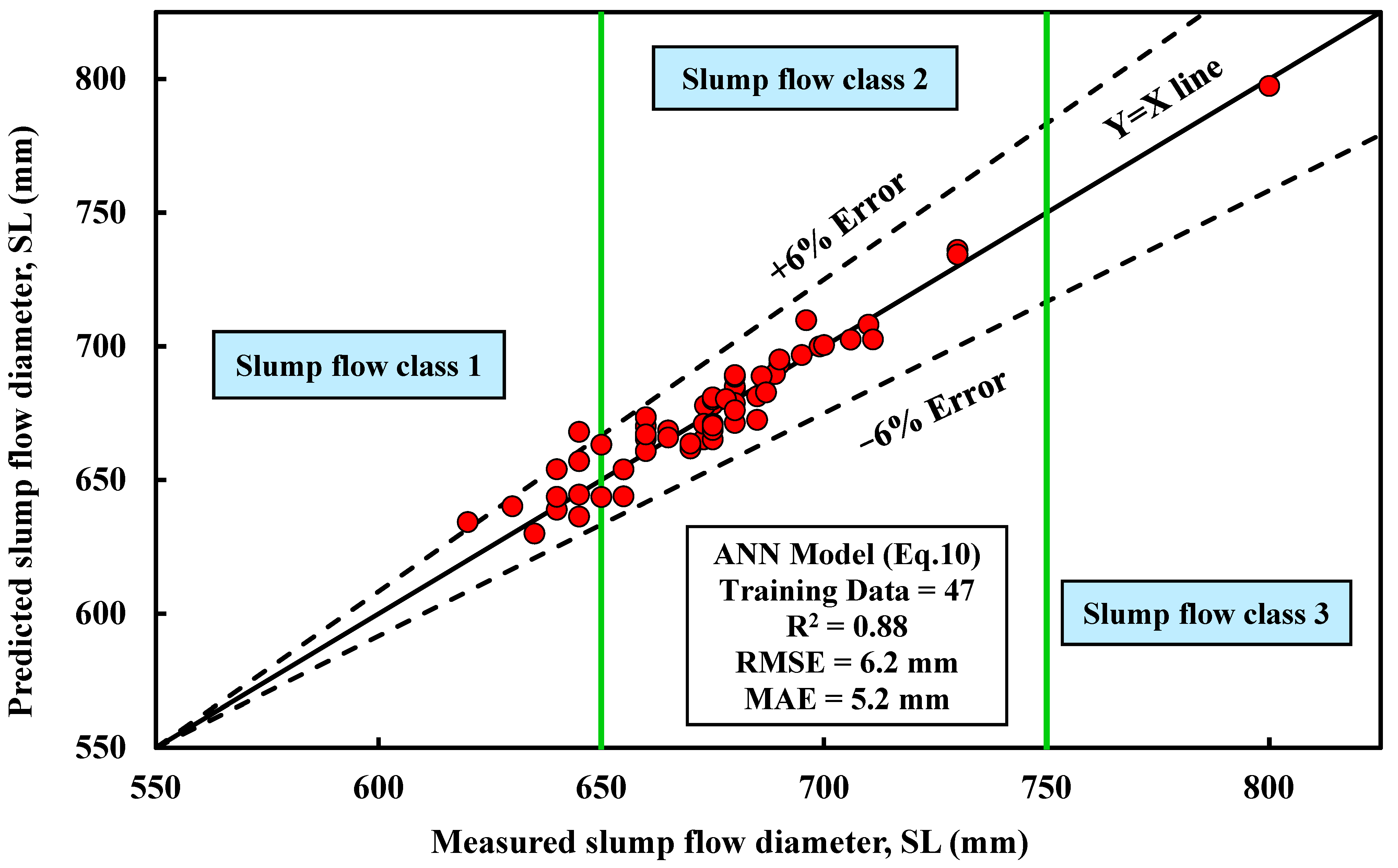
- The application of the Artificial Neural Network (ANN) model to different ranges of concrete strength (CS) and different classes of specimen length (SL) demonstrates its versatility and effectiveness. The higher CS strength range yielded more favorable outcomes, as indicated by an R2 (coefficient of determination) value of 0.79, an RMSE (Root Mean Square Error) of 4.13 MPa, and an MAE (Mean Absolute Error) of 2.98 MPa. These metrics signify a strong correlation and relatively low prediction errors, suggesting the model performed well in estimating axial strength for high CS levels. Overall, the reported R2 values demonstrated a good fit between the predicted and actual values, while the RMSE and MAE values indicated relatively small errors in the model’s predictions. These findings suggest that the ANN model can effectively capture the relationships between the CS, SL, and axial strength, highlighting its potential as a reliable tool for estimating concrete strength in various scenarios and ranges.
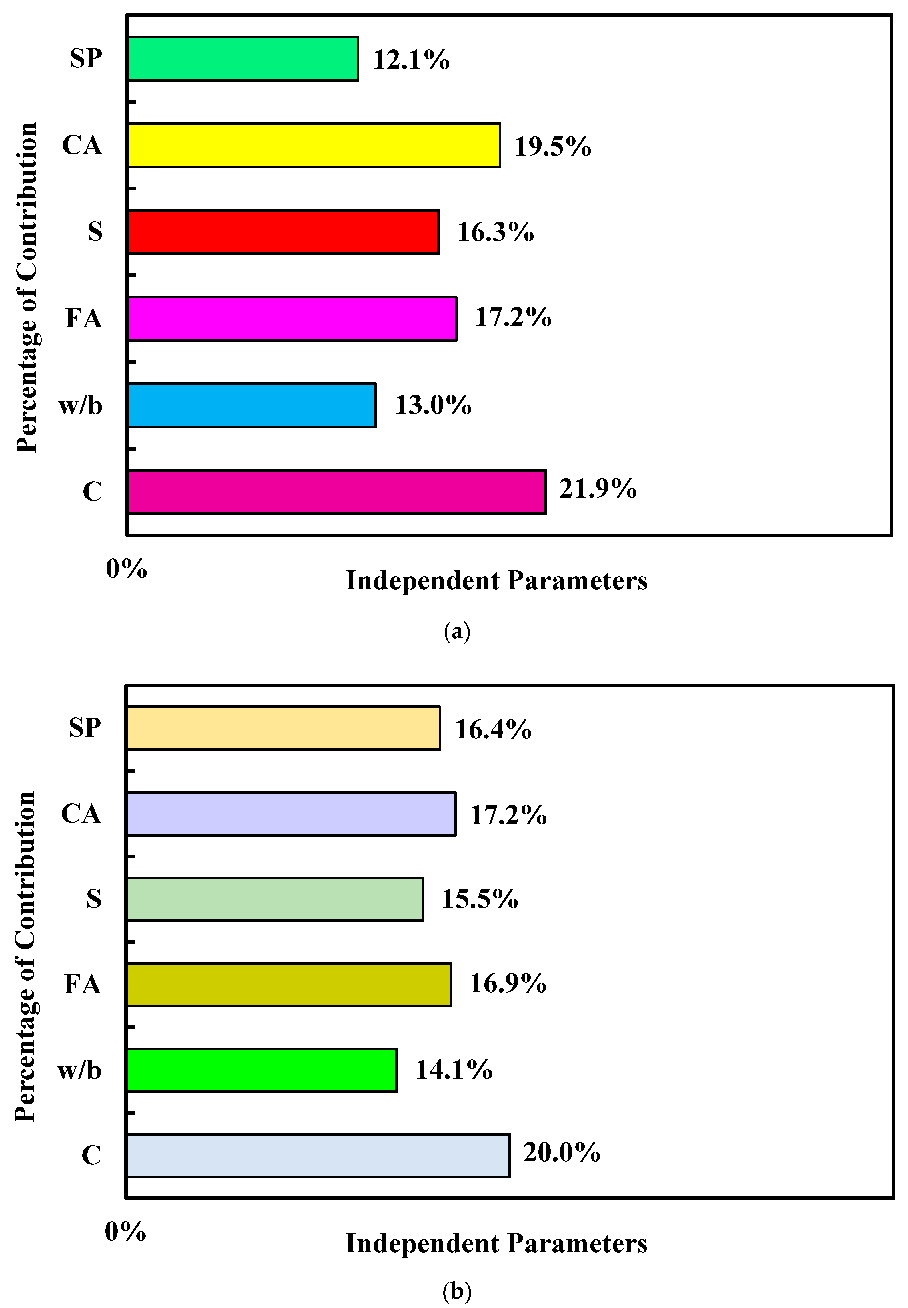
- Sensitivity analysis illustrates the cement content as the most effective parameter for both the CS and SL prediction of SCC.
7. Limitations and Future Work
- Other soft computing models should be used to predict the slump flow diameter and compressive strength of the fly ash-based self-compacted concrete.
- It is possible to assess other fly ash types and sources.
- The prediction of other types of workability tests can be investigated.
- Experiments need to be carried out to verify the produced models.
- It is also important to determine the effect of fly ash content on flexural and tensile strength.
Funding
Institutional Review Board Statement
Informed Consent Statement
Data Availability Statement
Conflicts of Interest
References
- Faraj, R.H.; Sherwani, A.F.H.; Daraei, A. Mechanical, fracture and durability properties of self-compacting high strength concrete containing recycled polypropylene plastic particles. J. Build. Eng. 2019, 25, 100808. [Google Scholar] [CrossRef]
- Faraj, R.H.; Sherwani, A.F.H.; Jafer, L.H.; Ibrahim, D.F. Rheological behavior and fresh properties of self-compacting high strength concrete containing recycled PP particles with fly ash and silica fume blended. J. Build. Eng. 2020, 34, 101667. [Google Scholar] [CrossRef]
- Faraj, R.H.; Ali, H.F.H.; Sherwani, A.F.H.; Hassan, B.R.; Karim, H. Use of recycled plastic in self-compacting concrete: A comprehensive review on fresh and mechanical properties. J. Build. Eng. 2020, 30, 101283. [Google Scholar] [CrossRef]
- Deilami, S.; Aslani, F.; Elchalakani, M. An experimental study on the durability and strength of SCC incorporating FA, GGBS and MS. Proc. Inst. Civ. Eng. Struct. Build. 2019, 172, 327–339. [Google Scholar] [CrossRef]
- Faraj, R.H.; Mohammed, A.A.; Mohammed, A.; Omer, K.M.; Ahmed, H.U. Systematic multiscale models to predict the compressive strength of self-compacting concretes modified with nanosilica at different curing ages. Eng. Comput. 2022, 38 (Suppl. 3), 2365–2388. [Google Scholar] [CrossRef]
- Neville, A.M.; Brooks, J.J. Concrete Technology; Longman Scientific & Technical: London, UK, 1987; pp. 242–246. [Google Scholar]
- Neville, A.M. Properties of Concrete; Longman Scientific & Technical: London, UK, 1995; Volume 4. [Google Scholar]
- Silvestre, J.; Silvestre, N.; De Brito, J. Review on concrete nanotechnology. Eur. J. Environ. Civil. Eng. 2016, 20, 455–485. [Google Scholar] [CrossRef]
- Karamoozian, A.; Karamoozian, M.; Ashrafi, H. Effect of Nano Particles on Self Compacting Concrete: An Experimental Study. Life Sci. J. 2013, 10, 95–101. [Google Scholar]
- Larsen, O.; Naruts, V.; Aleksandrova, O. Self-compacting concrete with recycled aggregates. Mater. Today Proc. 2019, 19, 2023–2026. [Google Scholar] [CrossRef]
- Ghasemi, M.; Ghasemi, M.R.; Mousavi, S.R. Studying the fracture parameters and size effect of steel fiber-reinforced self-compacting concrete. Constr. Build. Mater. 2019, 201, 447–460. [Google Scholar] [CrossRef]
- Ahmadi, M.A.; Alidoust, O.; Sadrinejad, I.; Nayeri, M. Development of mechanical properties of self compacting concrete contain rice husk ash. Int. J. Comput. Inf. Syst. Sci. Eng. 2007, 1, 259–262. [Google Scholar]
- Dinakar, P.; Manu, S.N. Concrete mix design for high strength self-compacting concrete using metakaolin. Mater. Des. 2014, 60, 661–668. [Google Scholar] [CrossRef]
- Güneyisi, E.; Gesoglu, M.; Al-Goody, A.; İpek, S. Fresh and rheological behavior of nano-silica and fly ash blended self-compacting concrete. Constr. Build. Mater. 2015, 95, 29–44. [Google Scholar] [CrossRef]
- Madandoust, R.; Ranjbar, M.M.; Ghavidel, R.; Shahabi, S.F. Assessment of factors influencing mechanical properties of steel fiber reinforced self-compacting concrete. Mater. Des. 2015, 83, 284–294. [Google Scholar] [CrossRef]
- Nikbin, I.M.; Beygi, M.H.A.; Kazemi, M.T.; Amiri, J.V.; Rahmani, E.; Rabbanifar, S.; Eslami, M. A comprehensive investigation into the effect of aging and coarse aggregate size and volume on mechanical properties of self-compacting concrete. Mater. Des. 2014, 59, 199–210. [Google Scholar] [CrossRef]
- Mahmood, W.; Mohammed, A. Performance of ANN and M5P-tree to forecast the compressive strength of hand-mix cement-grouted sands modified with polymer using ASTM and BS standards and evaluate the outcomes using SI with OBJ assessments. Neural Comput. Appl. 2022, 34, 15031–15051. [Google Scholar] [CrossRef]
- Asteris, P.G.; Lourenço, P.B.; Hajihassani, M.; Adami, C.-E.N.; Lemonis, M.E.; Skentou, A.D.; Marques, R.; Nguyen, H.; Rodrigues, H.; Varum, H. Soft computing based models for the prediction of masonry compressive strength. Eng. Struct. 2021, 248, 113276. [Google Scholar] [CrossRef]
- Rahimi, I.; Gandomi, A.H.; Asteris, P.G.; Chen, F. Analysis and prediction of COVID-19 using sir, seiqr and machine learning models: Australia, italy and uk cases. Information 2021, 12, 109. [Google Scholar] [CrossRef]
- Bardhan, A.; Gokceoglu, C.; Burman, A.; Samui, P.; Asteris, P.G. Efficient computational techniques for predicting the California bearing ratio of soil in soaked conditions. Eng. Geol. 2021, 291, 106239. [Google Scholar] [CrossRef]
- Ahmed, H.U.; Mohammed, A.S.; Mohammed, A.A.; Faraj, R.H. Systematic multiscale models to predict the compressive strength of fly ash-based geopolymer concrete at various mixture proportions and curing regimes. PLoS ONE 2021, 16, e0253006. [Google Scholar] [CrossRef]
- Koopialipoor, M.; Asteris, P.G.; Mohammed, A.S.; Alexakis, D.E.; Mamou, A.; Armaghani, D.J. Introducing stacking machine learning approaches for the prediction of rock deformation. Transp. Geotech. 2022, 34, 100756. [Google Scholar] [CrossRef]
- Ahmed, H.U.; Mohammed, A.S.; Faraj, R.H.; Abdalla, A.A.; Qaidi, S.M.; Sor, N.H.; Mohammed, A.A. Innovative modeling techniques including MEP, ANN and FQ to forecast the compressive strength of geopolymer concrete modified with nanoparticles. Neural Comput. Appl. 2023, 35, 12453–12479. [Google Scholar] [CrossRef]
- Asteris, P.G.; Ashrafian, A.; Rezaie-Balf, M. Prediction of the Compressive Strength of Self-Compacting Concrete using Surrogate Models. Comput. Concr. 2019, 24, 137–150. [Google Scholar]
- Emad, W.; Mohammed, A.S.; Bras, A.; Asteris, P.G.; Kurda, R.; Muhammed, Z.; Hassan, A.M.; Qaidi, S.M.A.; Sihag, P. Metamodel techniques to estimate the compressive strength of UHPFRC using various mix proportions and a high range of curing temperatures. Constr. Build. Mater. 2022, 349, 128737. [Google Scholar] [CrossRef]
- Mahmood, W.; Mohammed, A.S.; Asteris, P.G.; Kurda, R.; Armaghani, D.J. Modeling flexural and compressive strengths behaviour of cement-grouted sands modified with water reducer polymer. Appl. Sci. 2022, 12, 1016. [Google Scholar] [CrossRef]
- Asteris, P.G.; Koopialipoor, M.; Armaghani, D.J.; Kotsonis, E.A.; Lourenço, P.B. Prediction of Cement-based Mortars Compressive Strength using Machine Learning Techniques. Neural Comput. Appl. 2021, 33, 13089–13121. [Google Scholar] [CrossRef]
- Jaf, D.K.I.; Abdulrahman, P.I.; Abdulrahman, A.S.; Mohammed, A.S. Effitioned soft computing models to evaluate the impact of silicon dioxide (SiO2) to calcium oxide (CaO) ratio in fly ash on the compressive strength of concrete. J. Build. Eng. 2023, 74, 106820. [Google Scholar]
- Farooq, F.; Czarnecki, S.; Niewiadomski, P.; Aslam, F.; Alabduljabbar, H.; Ostrowski, K.A.; Śliwa-Wieczorek, K.; Nowobilski, T.; Malazdrewicz, S. A comparative study for the prediction of the compressive strength of self-compacting concrete modified with fly. Materials 2021, 14, 4934. [Google Scholar] [CrossRef]
- Patel, R.; Hossain, K.M.A.; Shehata, M.; Bouzoubaa, N.; Lachemi, M. Development of statistical models for mixture design of high-volume fly ash self-consolidating concrete. Mater. J. 2004, 101, 294–302. [Google Scholar]
- Ghezal, A.; Khayat, K.H. Optimizing self-consolidating concrete with limestone filler by using statistical factorial design methods. Mater. J. 2002, 99, 264–272. [Google Scholar]
- Sonebi, M. Applications of statistical models in proportioning medium-strength self-consolidating concrete. Mater. J. 2004, 101, 339–346. [Google Scholar]
- Sonebi, M. Medium strength self-compacting concrete containing fly ash: Modelling using factorial experimental plans. Cem. Concr. Res. 2004, 34, 1199–1208. [Google Scholar] [CrossRef]
- Sukumar, B.; Nagamani, K.; Raghavan, R.S. Evaluation of strength at early ages of self-compacting concrete with high volume fly ash. Constr. Build. Mater. 2008, 22, 1394–1401. [Google Scholar] [CrossRef]
- Bouzoubaâ, N.; Lachemi, M. Self-compacting concrete incorporating high volumes of class F fly ash: Preliminary results. Cem. Concr. Res. 2001, 31, 413–420. [Google Scholar] [CrossRef]
- Bui, V.K.; Akkaya, Y.; Shah, S.P. Rheological model for self-consolidating concrete. Mater. J. 2002, 99, 549–559. [Google Scholar]
- Güneyisi, E.; Gesoğlu, M.; Özbay, E. Strength and drying shrinkage properties of self-compacting concretes incorporating multi-system blended mineral admixtures. Constr. Build. Mater. 2010, 24, 1878–1887. [Google Scholar] [CrossRef]
- Pathak, N.; Siddique, R. Properties of self-compacting-concrete containing fly ash subjected to elevated temperatures. Constr. Build. Mater. 2012, 30, 274–280. [Google Scholar] [CrossRef]
- Jalal, M.; Mansouri, E. Effects of fly ash and cement content on rheological, mechanical, and transport properties of high-performance self-compacting concrete. Sci. Eng. Compos. Mater. 2012, 19, 393–405. [Google Scholar] [CrossRef]
- Dinakar, P.; Babu, K.G.; Santhanam, M. Mechanical properties of high-volume fly ash self-compacting concrete mixtures. Struct. Concr. 2008, 9, 109–116. [Google Scholar] [CrossRef]
- Dinakar, P. Design of self-compacting concrete with fly ash. Mag. Concr. Res. 2012, 64, 401–409. [Google Scholar] [CrossRef]
- Nehdi, M.; Pardhan, M.; Koshowski, S. Durability of self-consolidating concrete incorporating high-volume replacement composite cements. Cem. Concr. Res. 2004, 34, 2103–2112. [Google Scholar] [CrossRef]
- Barbhuiya, S. Effects of fly ash and dolomite powder on the properties of self-compacting concrete. Constr. Build. Mater. 2011, 25, 3301–3305. [Google Scholar] [CrossRef]
- Venkatakrishnaiah, R.; Sakthivel, G. Bulk utilization of flyash in self compacting concrete. KSCE J. Civil. Eng. 2015, 19, 2116–2120. [Google Scholar] [CrossRef]
- Sun, Z.J.; Duan, W.W.; Tian, M.L.; Fang, Y.F. Experimental research on self-compacting concrete with different mixture ratio of fly ash. In Advanced Materials Research; Trans Tech Publications Ltd.: Bäch, Switzerland, 2011; Volume 236, pp. 490–495. [Google Scholar]
- Ramanathan, P.; Baskar, I.; Muthupriya, P.; Venkatasubramani, R. Performance of self-compacting concrete containing different mineral admixtures. KSCE J. Civil. Eng. 2013, 17, 465–472. [Google Scholar] [CrossRef]
- Boel, V.; Audenaert, K.; De Schutter, G.; Heirman, G.; Vandewalle, L.; Desmet, B.; Vantomme, J. Transport properties of self compacting concrete with limestone filler or fly ash. Mater. Struct. 2007, 40, 507–516. [Google Scholar] [CrossRef]
- Douglas, R.P.; Bui, V.K.; Akkaya, Y.; Shah, S.P. Properties of Self-consolidating concrete containing class f fly ash: With a Verification of the minimum paste volume method. Spec. Publ. 2006, 233, 45–64. [Google Scholar]
- Bingöl, A.F.; Tohumcu, İ. Effects of different curing regimes on the compressive strength properties of self compacting concrete incorporating fly ash and silica fume. Mater. Des. 2013, 51, 12–18. [Google Scholar] [CrossRef]
- Hemalatha, T.; Ramaswamy, A.; Chandra Kishen, J.M. Micromechanical analysis of self compacting concrete. Mater. Struct. 2015, 48, 3719–3734. [Google Scholar] [CrossRef]
- Krishnapal, P.; Yadav, R.K.; Rajeev, C. Strength characteristics of self compacting concrete containing fly ash. Res. J. Eng. Sci. ISSN 2013, 2278, 9472. [Google Scholar]
- Dhiyaneshwaran, S.; Ramanathan, P.; Baskar, I.; Venkatasubramani, R. Study on durability characteristics of self-compacting concrete with fly ash. Jordan J. Civ. Eng. 2013, 7, 342–353. [Google Scholar]
- Siddique, R. Properties of self-compacting concrete containing class F fly ash. Mater. Des. 2011, 32, 1501–1507. [Google Scholar] [CrossRef]
- Mahalingam, B.; Nagamani, K. Effect of processed fly ash on fresh and hardened properties of self compacting concrete. Int. J. Earth Sci. Eng. 2011, 4, 930–940. [Google Scholar]
- Muthupriya, P.; Sri, P.N.; Ramanathan, M.P.; Venkatasubramani, R. Strength and workability character of self compacting concrete with GGBFS, FA and SF. Int. J. Emerg. Trends Eng. Dev. 2012, 2, 424–434. [Google Scholar]
- Siddique, R.; Aggarwal, P.; Aggarwal, Y. Influence of water/powder ratio on strength properties of self-compacting concrete containing coal fly ash and bottom ash. Constr. Build. Mater. 2012, 29, 73–81. [Google Scholar] [CrossRef]
- Gesoğlu, M.; Güneyisi, E.; Özbay, E. Properties of self-compacting concretes made with binary, ternary, and quaternary cementitious blends of fly ash, blast furnace slag, and silica fume. Constr. Build. Mater. 2009, 23, 1847–1854. [Google Scholar] [CrossRef]
- Nepomuceno, M.C.; Pereira-de-Oliveira, L.A.; Lopes, S.M.R. Methodology for the mix design of self-compacting concrete using different mineral additions in binary blends of powders. Constr. Build. Mater. 2014, 64, 82–94. [Google Scholar] [CrossRef]
- Gettu, R.; Izquierdo, J.; Gomes, P.C.C.; Josa, A. Development of high-strength self-compacting concrete with fly ash: A four-step experimental methodology. In Proceedings of the 27th Conference on Our World in Concrete & Structures, Singapore, 29–30 August 2002; Tam, C.T., Ho, D.W., Paramasivam, P., Tan, T.H., Eds.; Premier Pte. Ltd.: Singapore, 2002; pp. 217–224. [Google Scholar]
- Şahmaran, M.; Yaman, İ.Ö.; Tokyay, M. Transport and mechanical properties of self consolidating concrete with high volume fly ash. Cem. Concr. Compos. 2009, 31, 99–106. [Google Scholar] [CrossRef]
- Liu, M. Self-compacting concrete with different levels of pulverized fuel ash. Constr. Build. Mater. 2010, 24, 1245–1252. [Google Scholar] [CrossRef]
- Piro, N.S.; Mohammed, A.S.; Hamad, S.M.; Kurda, R.; Qader, B.S. Multifunctional computational models to predict the long-term compressive strength of concrete incorporated with waste steel slag. Struct. Concr. 2023, 24, 2093–2112. [Google Scholar] [CrossRef]
- Piro, N.S.; Mohammed, A.; Hamad, S.M.; Kurda, R. Artificial neural networks (ANN), MARS, and adaptive network-based fuzzy inference system (ANFIS) to predict the stress at the failure of concrete with waste steel slag coarse aggregate replacement. Neural Comput. Appl. 2023, 35, 13293–13319. [Google Scholar] [CrossRef]
- Ibrahim, A.K.; Dhahir, H.Y.; Mohammed, A.S.; Omar, H.A.; Sedo, A.H. The effectiveness of surrogate models in predicting the long-term behavior of varying compressive strength ranges of recycled concrete aggregate for a variety of shapes and sizes of specimens. Arch. Civil. Mech. Eng. 2023, 23, 61. [Google Scholar] [CrossRef]
- Ahmed, A.; Abubakr, P.; Mohammed, A.S. Efficient models to evaluate the effect of C3S, C2S, C3A, and C4AF contents on the long-term compressive strength of cement paste. Structures 2023, 47, 1459–1475. [Google Scholar] [CrossRef]
- Mohammed, A.; Rafiq, S.; Sihag, P.; Mahmood, W.; Ghafor, K.; Sarwar, W. ANN, M5P-tree model, and nonlinear regression approaches to predict the compression strength of cement-based mortar modified by quicklime at various water/cement ratios and curing times. Arab. J. Geosci. 2020, 13, 1216. [Google Scholar] [CrossRef]
- Mohammed, A.; Rafiq, S.; Sihag, P.; Kurda, R.; Mahmood, W. Soft computing techniques: Systematic multiscale models to predict the compressive strength of HVFA concrete based on mix proportions and curing times. J. Build. Eng. 2021, 33, 101851. [Google Scholar] [CrossRef]
- Mohammed, A.S.; Emad, W.; Sarwar Qadir, W.; Kurda, R.; Ghafor, K.; Kadhim Faris, R. Modeling the Impact of Liquid Polymers on Concrete Stability in Terms of a Slump and Compressive Strength. Appl. Sci. 2023, 13, 1208. [Google Scholar] [CrossRef]
- Ali, R.; Muayad, M.; Mohammed, A.S.; Asteris, P.G. Analysis and prediction of the effect of Nanosilica on the compressive strength of concrete with different mix proportions and specimen sizes using various numerical approaches. Struct. Concr. 2022, 24, 4161–4184. [Google Scholar] [CrossRef]
- Abdalla, A.; Mohammed, A.S. Hybrid MARS-, MEP-, and ANN-based prediction for modeling the compressive strength of cement mortar with various sand size and clay mineral metakaolin content. Arch. Civil. Mech. Eng. 2022, 22, 194. [Google Scholar] [CrossRef]
- Asteris, P.G.; Nozhati, S.; Nikoo, M.; Cavaleri, L.; Nikoo, M. Krill herd algorithm-based neural network in structural seismic reliability evaluation. Mech. Adv. Mater. Struct. 2019, 26, 1146–1153. [Google Scholar] [CrossRef]
- Asteris, P.G.; Lemonis, M.E.; Le, T.-T.; Tsavdaridis, K.D. Evaluation of the ultimate eccentric load of rectangular CFSTs using advanced neural network modeling. Eng. Struct. 2021, 248, 113297. [Google Scholar] [CrossRef]
- Asteris, P.G.; Lourenço, P.B.; Adami, C.A.; Roussis, P.C.; Armaghani, D.J.; Cavaleri, L.; Chalioris, C.E.; Hajihassani, M.; Lemonis, M.E.; Mohammed, A.S.; et al. Revealing the nature of metakaolin-based concrete materials using Artificial Intelligence Techniques. Constr. Build. Mater. 2022, 322, 126500. [Google Scholar] [CrossRef]
- Asteris, P.G.; Armaghani, D.J.; Hatzigeorgiou, G.D.; Karayannis, C.G.; Pilakoutas, K. Predicting the shear strength of reinforced concrete beams using Artificial Neural Networks. Computers and Concrete. An. Int. J. 2019, 24, 469–488. [Google Scholar]
- Armaghani, D.J.; Asteris, P.G. A comparative study of ANN and ANFIS models for the prediction of cement-based mortar materials compressive strength. Neural Comput. Appl. 2021, 33, 4501–4532. [Google Scholar] [CrossRef]
- Mohammed, A.; Kurda, R.; Armaghani, D.J.; Hasanipanah, M. Prediction of compressive strength of concrete modified with fly ash: Applications of neuro-swarm and neuro-imperialism models. Comput. Concr. 2021, 27, 489. [Google Scholar]
- Qadir, W.; Ghafor, K.; Mohammed, A. Evaluation the effect of lime on the plastic and hardened properties of cement mortar and quantified using Vipulanandan model. Open Eng. 2019, 9, 468–480. [Google Scholar] [CrossRef]
- Sarwar, W.; Ghafor, K.; Mohammed, A. Regression analysis and Vipulanandan model to quantify the effect of polymers on the plastic and hardened properties with the tensile bonding strength of the cement mortar. Results Mater. 2019, 1, 100011. [Google Scholar] [CrossRef]
- Qaidi, S.; Al-Kamaki, Y.S.; Al-Mahaidi, R.; Mohammed, A.S.; Ahmed, H.U.; Zaid, O.; Althoey, F.; Ahmad, J.; Isleem, H.F.; Bennetts, I. Investigation of the effectiveness of CFRP strengthening of concrete made with recycled waste PET fine plastic aggregate. PLoS ONE 2022, 17, e0269664. [Google Scholar] [CrossRef]
- Abdalla, A.A.; Salih Mohammed, A. Theoretical models to evaluate the effect of SiO2 and CaO contents on the long-term compressive strength of cement mortar modified with cement kiln dust (CKD). Arch. Civ. Mech. Eng. 2022, 22, 105. [Google Scholar] [CrossRef]
- Barkhordari, M.S.; Armaghani, D.J.; Mohammed, A.S.; Ulrikh, D.V. Data-driven compressive strength prediction of fly ash concrete using ensemble learner algorithms. Buildings 2022, 12, 132. [Google Scholar] [CrossRef]
- Piro, N.S.; Salih, A.; Hamad, S.M.; Kurda, R. Comprehensive multiscale techniques to estimate the compressive strength of concrete incorporated with carbon nanotubes at various curing times and mix proportions. J. Mater. Res. Technol. 2021, 15, 6506–6527. [Google Scholar] [CrossRef]


| Parameter | Equation | Range | Best Value |
|---|---|---|---|
| [58,80] | 1 | ||
| [24,80] | 0 | ||
| [24,69] | 0 | ||
| [58,80] | 0 | ||
| [69,80] | <0.1 | Excellent | |
| 0.1 to 0.2 | Good | ||
| 0.2 to 0.3 | fair | ||
| >0.3 | Poor |
| Compressive strength | Model | Figure (No) | Equation (No.) | Training | Testing | Ranking | ||||
|---|---|---|---|---|---|---|---|---|---|---|
| R² | RMSE (MPa) | MAE (MPa) | R² | RMSE (MPa) | MAE (MPa) | |||||
| NLR | 7a | 5 | 0.81 | 5.82 | 4.67 | 0.84 | 7.67 | 4.72 | 2 | |
| MLR | 8a | 7 | 0.81 | 6.04 | 4.69 | 0.82 | 7.92 | 4.65 | 3 | |
| ANN | 11a | 9 | 0.94 | 3.56 | 2.54 | 0.95 | 3.49 | 2.45 | 1 | |
| Slump flow diameter | Model | Figure (No) | Equation (No.) | Training | Testing | Ranking | ||||
| R² | RMSE (mm) | MAE (mm) | R² | RMSE (mm) | MAE (mm) | |||||
| NLR | 7b | 6 | 0.82 | 11.6 | 10.12 | 0.57 | 27.4 | 27.1 | 3 | |
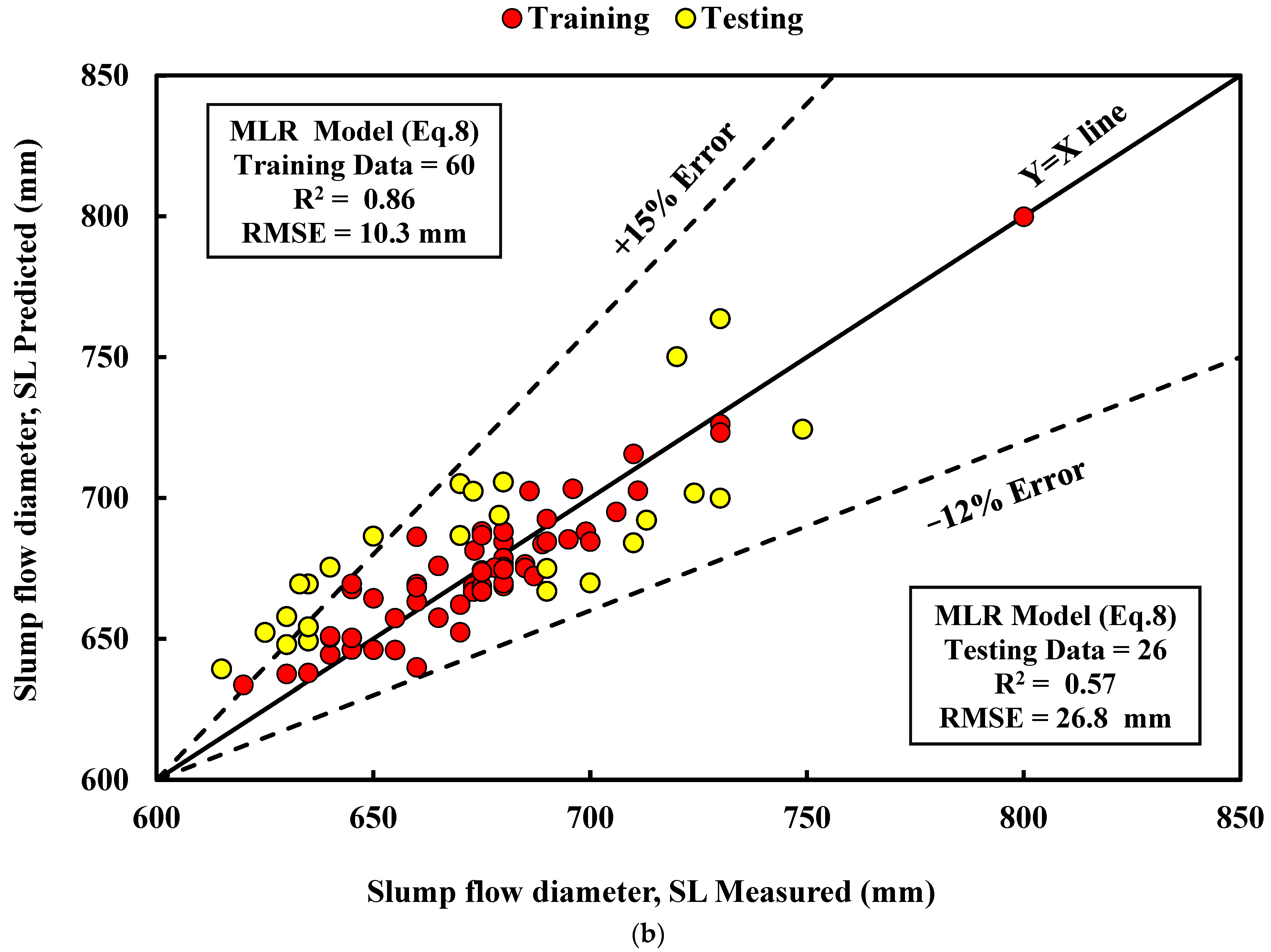
| MLR | 8b | 8 | 0.86 | 10.3 | 8.54 | 0.57 | 26.8 | 25.93 | 2 | |
| ANN | 11b | 10 | 0.93 | 7.5 | 5.97 | 0.997 | 2.2 | 1.39 | 1 | |
Disclaimer/Publisher’s Note: The statements, opinions and data contained in all publications are solely those of the individual author(s) and contributor(s) and not of MDPI and/or the editor(s). MDPI and/or the editor(s) disclaim responsibility for any injury to people or property resulting from any ideas, methods, instructions or products referred to in the content. |
© 2023 by the author. Licensee MDPI, Basel, Switzerland. This article is an open access article distributed under the terms and conditions of the Creative Commons Attribution (CC BY) license (https://creativecommons.org/licenses/by/4.0/).
Share and Cite
Ismael Jaf, D.K. Soft Computing and Machine Learning-Based Models to Predict the Slump and Compressive Strength of Self-Compacted Concrete Modified with Fly Ash. Sustainability 2023, 15, 11554. https://doi.org/10.3390/su151511554
Ismael Jaf DK. Soft Computing and Machine Learning-Based Models to Predict the Slump and Compressive Strength of Self-Compacted Concrete Modified with Fly Ash. Sustainability. 2023; 15(15):11554. https://doi.org/10.3390/su151511554
Chicago/Turabian StyleIsmael Jaf, Dilshad Kakasor. 2023. "Soft Computing and Machine Learning-Based Models to Predict the Slump and Compressive Strength of Self-Compacted Concrete Modified with Fly Ash" Sustainability 15, no. 15: 11554. https://doi.org/10.3390/su151511554
APA StyleIsmael Jaf, D. K. (2023). Soft Computing and Machine Learning-Based Models to Predict the Slump and Compressive Strength of Self-Compacted Concrete Modified with Fly Ash. Sustainability, 15(15), 11554. https://doi.org/10.3390/su151511554