Article

Digital Model of Deflection of a Cable-Stayed Bridge Driven by Deep Learning and Big Data Optimized via PCA-LGBM

1
Hong Kong-Zhuhai-Macao Bridge Authority, Zhuhai 519060, China
2
Key Laboratory of Concrete and Prestressed Concrete Structures of Ministry of Education, Southeast University, Nanjing 210096, China
3
Shenzhen Express Engineering Consulting Co., Ltd., Shenzhen 518000, China
*
Author to whom correspondence should be addressed.
Sustainability 2023, 15(12), 9623; https://doi.org/10.3390/su15129623
Submission received: 5 April 2023 / Revised: 12 June 2023 / Accepted: 13 June 2023 / Published: 15 June 2023
(This article belongs to the Special Issue Artificial Intelligence (AI) in Structural Health Monitoring)

Abstract

:
Based on big data, we can build a regression model between a temperature field and a temperature-induced deflection to provide a control group representing the service performance of bridges, which has a positive effect on the full life cycle maintenance of bridges. However, the spatial temperature information of a cable-stayed bridge is difficult to describe. To establish a regression model with high precision, the improved PCA-LGBM (principal component analysis and light gradient boosting machine) algorithm is proposed to extract the main temperature features that can reflect the spatial temperature information as accurately and efficiently as possible. Then, in this article, we searched for a suitable digital tool for modeling the regressive relationship between the temperature variables and the temperature-induced deflection of a cable-stayed bridge. The multiple linear regression model has relatively low precision. The precision of the backpropagation neural network (BPNN) model has been improved, but it is still unsatisfactory. The nested long short-term memory (NLSTM) model improves the nonlinear expression ability of the regression model and is more precise than BPNN models and the classical LSTM. The architecture of the NLSTM network is optimized for high precision and to avoid the waste of computational costs. Based on the four main temperature features extracted via the PCA-LGBM, the NLSTM network with double hidden layers and 256 hidden units in each hidden layer has much higher precision than the other regression models. For the NLSTM regression model of the temperature-induced deflection of a cable-stayed bridge, the mean absolute error is only 4.76 mm, and the mean square error is only 18.57 mm2. The control value of the NLSTM regression model is precise and thus provides the potential for early detection of bridge anomalies. This article can provide reference processes and a data extraction algorithm for deflection modeling of other cable-stayed bridges.

1. Introduction

Cable-stayed bridges are common long-span bridges that are increasingly becoming widely used. To ensure the safety of cable-stayed bridges for the full life cycle, structural health monitoring (SHM) systems can be installed to monitor the use status of bridges to avert economic and safety risks caused by destructive cable-stayed bridge accidents [1,2]. We can effectively use big data to mine crucial information and detect bridge health state through the SHM system. In the full life cycle of the structure, deflection is a control index reflecting mechanical properties [3]. In the operation phase, the most critical factors affecting the vertical deflection of the main girder are temperature and vehicle load; however, the impact of thermal load is more significant [4,5]. Accordingly, we can establish a correlation model between temperature and deflection induced by temperature. By inputting the real-time temperature data from the SHM system, we can obtain the output data of deflection induced by temperature and use the output data as control values. The normal working state of the bridge can then be evaluated according to the difference between its deflection and the control value. Efficient evaluation of bridges will facilitate the prolonging life of bridges as early as possible, and the longer bridge service life will obviously benefit the sustainability of infrastructures. Therefore, a high-precision model that provides reliable deflection control values is urgently required [6].
Naturally, the temperature of the girder affects its deflection [7], which is also affected by the temperature of the bridge tower [8,9]. The spatial temperature information is very complex; hence, efficiently and accurately extracting the temperature features required for establishing the regression model is difficult. In the existing analytic model, even if the composite effect of multiple temperatures is considered, large errors occur [9]. Benefiting from the wide application of SHM systems, a large amount of environmental information and bridge response data were collected [10]. These data have a volume of several months, the velocity of real-time bridge information, and a variety of different sensors. Therefore, the data obtained via the SHM system is obviously big data that contain potential information about the service performance of the bridge [10,11].
The information contained in bridge monitoring data is very valuable; therefore, utilizing big data to promote bridge engineering research has become the general trend [1,12]. If an accurate regression model can be established between temperature field and temperature deflection based on the monitoring big data of a cable-stayed bridge, the regression value of this model can be used as the control group when the bridge works normally. To establish the model with satisfactory precision, the main temperature features must be extracted from the collected temperature field information for removing redundant information, and thus the corresponding extraction algorithms should be developed. The temperature-induced deflection of cable-stayed bridges is very complex. To ensure that the mapping relationship between temperature and temperature-induced deflection can be precisely expressed through regression modeling, deep learning technology should be applied to satisfy the high-precision regression model.
Firstly, for optimal precision, the temperature feature extraction method combining two intelligent algorithms is proposed in this paper. The principle component analysis (PCA) algorithm is usually used for restructuring temperature field data into several main temperature features; the restructured data features obtained via PCA can better adapt to nonlinear modeling [13], but the redundant features must be removed. Therefore, in this paper, light gradient boosting machine (LGBM), which belongs to machine learning technology and is able to better explain the nonlinear connections between data features [14], is further used to select the most useful features from the data information reconstructed via PCA.
Then, to determine the appropriate deep learning modeling tool, this paper tested different neural networks and the network with the best performance was selected. The traditional backpropagation neural network (BPNN) [15] with the typical back propagation characteristic [16] was tested; the advanced nested long short-term memory (NLSTM) network that can express highly nonlinear temporal relationship [17] was tested; and the classic LSTM network [18] was also tested to prove that NLSTM is more suitable for the mapping model in this paper. Meanwhile, the paper explores the optimal architecture of neural networks with the comprehensive consideration of effect and cost.
Finally, the digital regression model built by using the deep neural network can achieve a very high precision, thus providing a valuable control group for bridge deflection; therefore, the abnormal state of the bridge can be detected as early as possible, which has a positive significance for bridge health monitoring.
In this paper, Section 2 introduces the extraction of the datasets of temperature features and temperature-induced deflection, and the combined PCA-LGBM algorithm for extracting the temperature features is described. In Section 3, the multiple linear regression model is built to map the relationship between the temperature features and the temperature-induced deflection. In Section 4, the BPNN is used to preliminarily improve precision of the regression model. In Section 5, the deep learning NLSTM model is built to achieve higher precision and NLSTM is proved to be more precise than the classic LSTM. In Section 6, the performances of different digital models are discussed for selecting the best modeling scheme. Section 7 provides the summary and conclusions of this paper.

2. Extraction of Temperature Features and Temperature-Induced Deflection

2.1. Bridge and Monitoring System

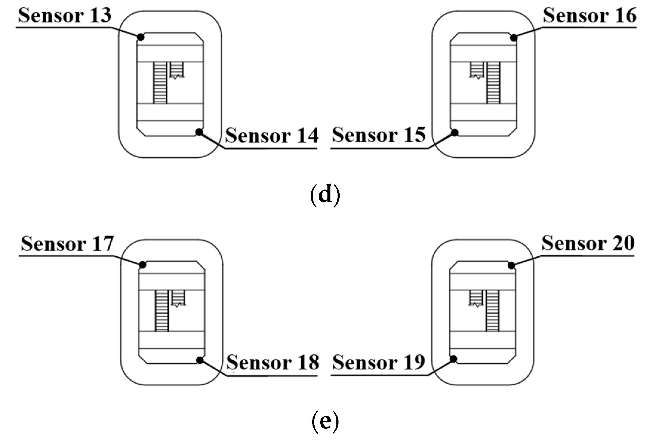
This research is based on data from the SHM system of a sea-crossing bridge between Macau and Hong Kong. As shown in Figure 1a, the bridge has a total length of 1150 m and a main span of 456 m. The main girders are steel box beams measuring 36 m in width and 4.6 m in height. As shown in Figure 1b, the bridge towers adopt the concrete structure with a box section, and the two towers are 163 m high. As shown in Figure 1c, there are twelve temperature sensors installed in the main girder and these temperature sensors are denoted as sensor 1 to sensor 12, and there is a deflection sensor in the center of the main girder. As shown in Figure 1d,e, there are eight temperature sensors installed in the concrete structure of the two bridge towers, and these temperature sensors are denoted as sensor 13 to sensor 20.

2.2. Temperature-Induced Deflection

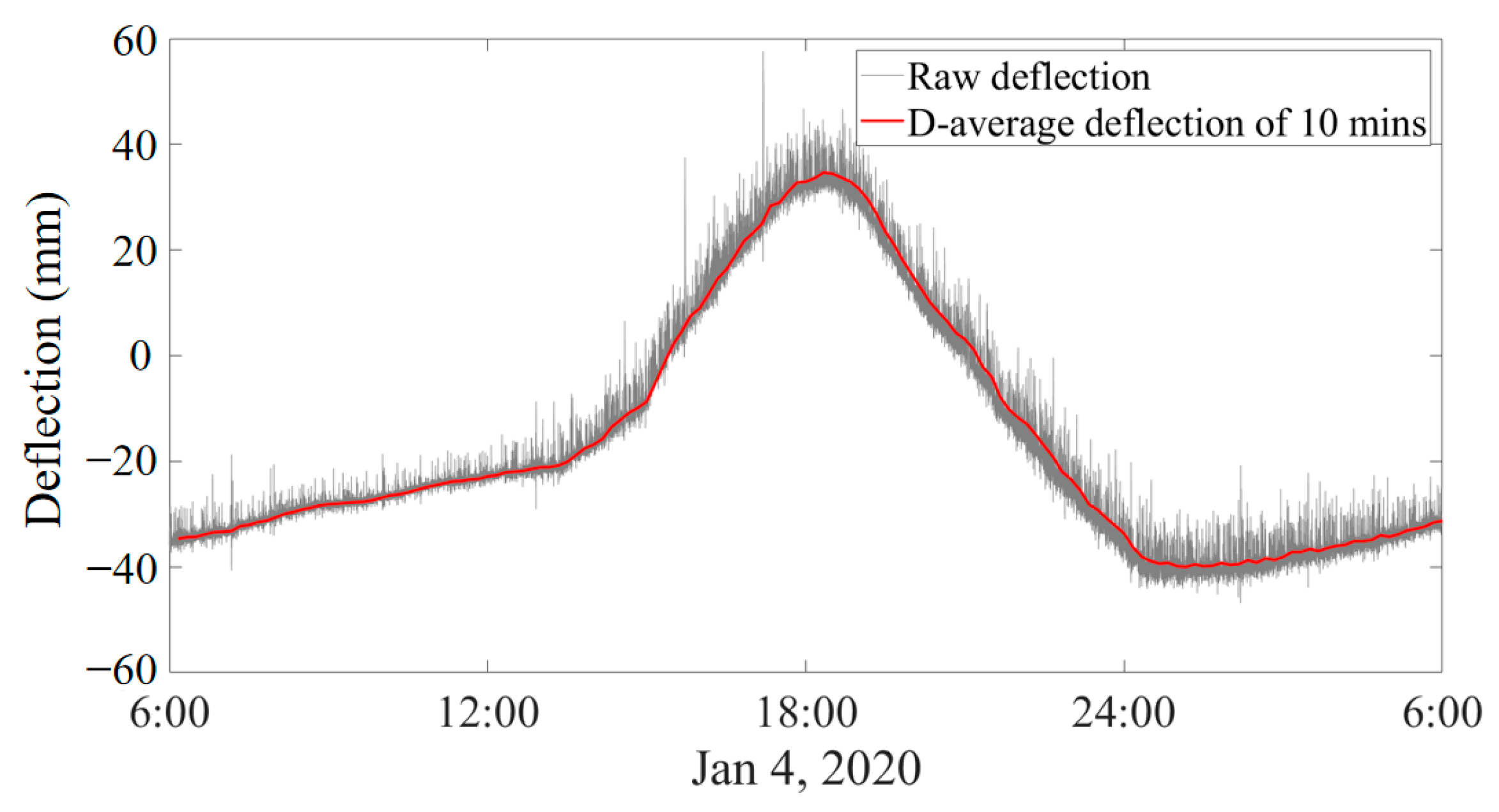
Figure 2 shows the deflection of the main girder on 4 January 2020. The existing studies found that averaging the deflection data every ten minutes can properly eliminate the effects of dynamic loads [19]. Therefore, the ten-minute time window is used to average the original deflection data, thus obtaining the temperature-induced deflection named D. In Figure 2, the increase in deflection indicates that the main girder is up-warped, and the decrease in deflection represents the downward deformation of the main girder. Around 12:00, the temperature of the bridge reaches its peak, and the temperature-induced deflection also reaches its extreme point.
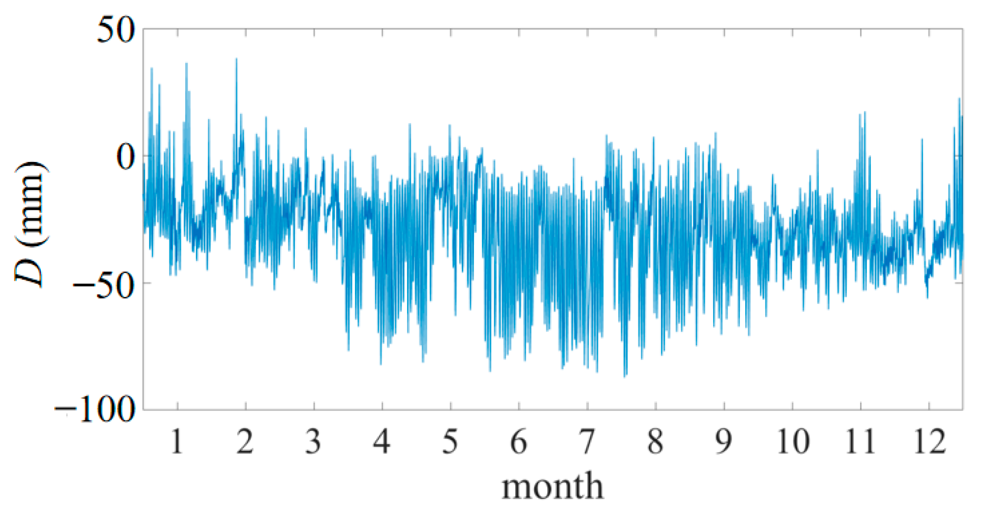
Figure 3 shows the deflection change during one year after the ten-minute average processing. The temperature-induced deflection of the main girder is influenced by the complex temperature field distributed in the entire bridge, and different temperature factors have different effects on the deflection. For example, the effect of the overall temperature change in the main girder and the vertical temperature difference of the main girder is opposite when producing the deflection. At the same time, the spatial–temporal distribution of the temperature field is very complex and results in temperature changes in different parts varying greatly over a daily or longer period. Therefore, although the trend of temperature-induced deflection in Figure 3 is generally consistent with temperature, it has distinctive spatial–temporal characteristics rather than fully adapting to temperature change. The complex temperature field data must be processed to achieve the optimal regression modeling between the temperature variables and the temperature-induced deflection. Next, we will introduce the processing of temperature data.

2.3. Temperature Information

To correspond to the time interval of the temperature-induced deflection, we also averaged the data of the temperature sensor every ten minutes. Figure 4 shows the temperature data of sensors 4, 7, 11, and 18 during a one year period after the ten-minute average processing. This bridge is located between Hong Kong and Macau, so the temperature did not fall below 0 °C throughout the year. Sensor 4 is located at the top plate of the main girder and, because of the sunlight exposure, its temperature extremes and temperature changes are more than other sensors. Both sensor 11 and sensor 12 are located at the bottom plate of the main girder and, due to its location receiving less sunlight exposure, the measured temperatures of these two sensors are relatively small. Sensor 18 is installed in the concrete of the tower in order to measure the temperature of the tower. Both the extremes and the changes in the temperature of the tower are smaller than those of the main girder because the tower has a very sturdy cross-section.
The temperature variables of the 20 sensors after processing are named T1~T20. Taking all the temperature variables as the input data for modeling not only wastes a lot of computing cost but may have a negative impact because there exists the obvious information redundancy between the temperature measured via different sensors. The datasets collected via these temperature sensors are similar but have independent significance. Therefore, these data cannot be randomly selected or discarded; thus, all the temperature data need to be restructured in order to extract the main temperature features as the input data of the regression model.

2.4. Extraction of Temperature Features

2.4.1. Information Reconstruction via Principal Component Analysis (PCA)

PCA can recombine the multiple measured information into new variables that are independent of each other [20]. Therefore, it can reconstruct the data according to the actual situation. Some of the reconstructed variables will contain a lot of effective information, while the other variables are redundant information that can be removed.
If there are n parameters, the centralized parameters can form a matrix  W = [ w 1 , w 2 , w 3 , , w n ] . The  w n  is described by Equation (1):
w n = [ w n 1 , w n 2 , w n 3 , , w n k ] T
where k is the amount of data.
The orthogonal group that forms a new mapping space is  { u 1 , u 2 , u 3 , , u k } , and the projection of the original characteristic parameter  w i  in  u j  can be described as  w i T u j . The variance in the original data after the projection in  u j  can be described by Equation (2):
J j = 1 n i = 1 n ( w i T u j ) 2 = u j T n W W T u j
S is the covariance matrix of W. It is described by Equation (3):
S = W W T / n
The solution to the projection space can be converted into Equation (4):
max J j = u j T S u j s . t . u j T u j = 1
According to the Lagrangri multiplier method, Equation (5) can be constructed:
F ( u j ) = u j T S u j + λ j ( 1 u j T u j )
Taking the derivative of function F, the result is described by Equation (6):
F u j = 2 S u j - 2 λ j u j = 0 S u j = λ j u j
where  λ j  is the eigenvalue and  u j  is the eigenvector of S.
The eigenvectors are composed of a matrix  U = [ u 1 , u 2 , u 3 , , u j ] . The matrix of reconstructed information can be described by Equation (7):
B = [ b 1 , b 2 , b 3 , , b j ] = W U
The column vector bj is the reconstructed vector.
Based on the PCA algorithm, the principal components are orthogonal and non-correlated. Through this method, the reconstruction of the temperature variables can be performed efficiently and accurately. The temperature variables obtained by the reconstruction are named T1~T20′. In the regression modeling of temperature deflection, these temperature variables reconstructed via PCA have different information abundances; therefore, the relevant algorithm must be further used to analyze the information contribution of different features in order to retain the most useful information and remove redundant data. Subsequent work revolves around the light gradient boosting machine framework.

2.4.2. Analysis of the Reconstructed Information via Light Gradient Boosting

Machine (LGBM)

GBDT (Gradient Boosting Decision Tree) is the classical and reliable analytical method belonging to machine learning. As the improved framework based on the GBDT algorithm, LGBM can reduce the computational cost by parallel training and thus be widely used in data mining [21].
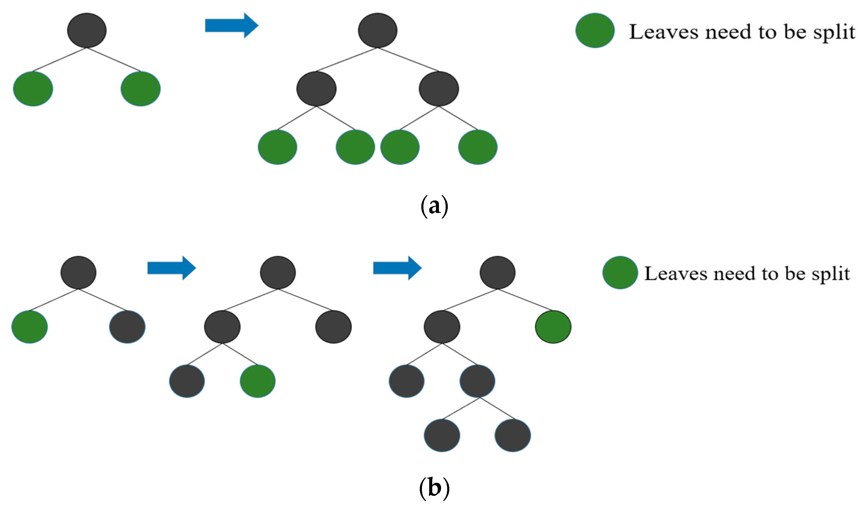
Similar to the GBDT, LGBM implements the decision tree by dividing the histogram of the original data. However, LGBM has been further optimized by replacing the traditional level-wise algorithm by the leaf-wise algorithm with depth constraints. The leaf-wise algorithm splits the leaf with the most profit first. Therefore, the leaf-wise algorithm can reduce errors and improve accuracy.
Since the growth of the leaf-wise is not limited and prone to overfitting, LGBM adds the limit of the maximum depth to prevent overfitting. Figure 5 shows the difference between the level-wise algorithm and the leaf-wise algorithm. Therefore, the LGBM algorithm can accurately sort the importance of different variables by the decision tree scheme.
The reconstructed temperature variables obtained via PCA are completely uncorrelated. However, the information contribution of the different variables to the deflection regression is not the same. As the number of input features to the regression model increases, information redundancy also increases. The redundancy not only influences the computational cost, but also reduces the precision of the regression model.
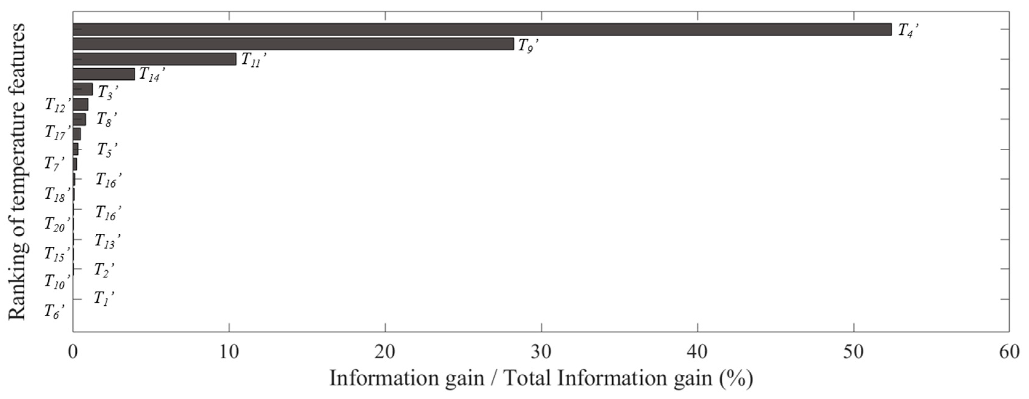
Through the PCA algorithm, the reconstructed temperature variables T1~T20 have been obtained. Here LGBM is used for selecting the most effective temperature features. The calculation process is shown as follows:
Step 1: Put the temperature variables T1~T20’ from PCA into the LGBM processing module. The LGBM module will calculate Ii, which is the information gain of the temperature variable Ti′. The value of the information gain represents the importance of this variable.
Step 2: Rank the temperature variable Ti in descending order according to the Ii obtained in Step 1.
Step 3: Select temperature variables in order of information gain from high to low until the sum of the information gains reaches 95%.
The selected temperature variables obtained by Step 3 contain the optimal information abundance and are used as the input features for building the regression model.

2.4.3. Extraction Process of the Temperature Features via PCA-LGBM

Data from the health monitoring system between January 2020 and December 2020 are used. T1~T20 are the restructured temperature variables via PCA. The information gains of T1~T20 are calculated via LGBM. Figure 6 shows the ratio between the information gain and the total information gain of T1~T20. To retain the original information as much as possible while reducing the computational cost, T4, T9, T11′, and T14, which include more than 95% of the total information gain, are selected as the input features of the regression model and are renamed Ta, Tb, Tc, and Td. From January to December, each temperature feature retains 47,520 data points. Figure 7 shows the time–history curves of the four temperature features.

2.5. Training Set and Test Set

We could use the deflection data D and the temperature features Ta, Tb, Tc, and Td to establish a regression model. To make the model have high precision and generalization performance, dividing the 47,520 data points of the deflection dataset D into the training set D1 contains 38,016 (80%) data points for the iterative training, and dividing the test set D2 contains 9504 (20%) data points for testing the regression model. Correspondingly, for the temperature features Ta, Tb, Tc, and Td, every 38,016 data points extracted are used to form the training sets Ta1, Tb1, Tc1, and Td1 to coordinate with the training set D1, and every 9504 data points extracted are used to form the test sets Ta2, Tb2, Tc2, and Td2 to coordinate with the test set D2.

2.6. Constructing the Data Mode for Neural Networks

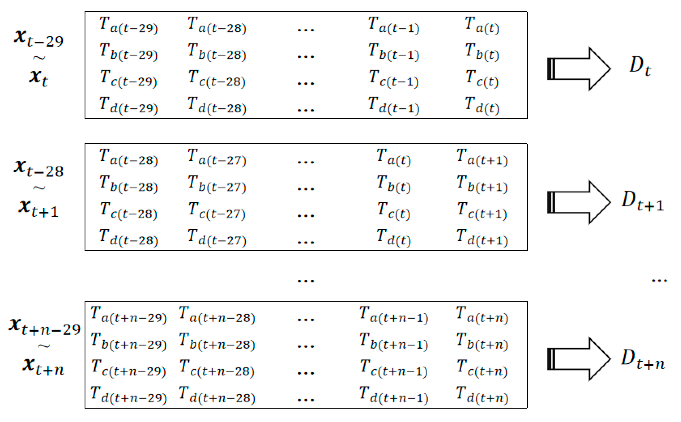
According to the above, we can form the input data as the dataset  X = { x 1 , x 2 , , x t } . The  x t  is described by Equation (8).
x t = T a ( t )   T b ( t )   T c ( t )   T d ( t )
According to the existing research result, when building the mapping model of temperature and temperature-induced response via neural networks, using the temperature data of the first five hours as input data and the response data of the current moment as output data, the model will obtain the highest generalization performance [22]. Therefore, the data flow shown in Figure 8 is constructed as the input–output mode for establishing the regression model. As shown in Figure 8, when the deflection Dt at time t is needed to be fitted, the thirty arrays of the current and previous moments from the dataset X are input. With the passage of time, this mapping mode also constantly changes as shown in Figure 8.

3. Multiple Linear Regression (MLR) Analysis

The four temperature features, Ta, Tb, Tc, and Td, together influence the temperature-induced deflection. We used them as the input variables and used D as the output variable for the MLR modeling. The goodness of fit  R 2  and mean square error (MSE) were used for evaluating the precision of the regression model. The calculation formula established via multiple linear regression analysis is described by Equation (9):
D = 1.8850 T a + 4.0521 T b + 7.2960 T c + 11.0852 T d 30.4653
where  D  is the regression value of the temperature-induced deflection.
The goodness of fit R2 is described by Equation (10):
R 2 = n = 1 N ( D n D ¯ ) 2 n = 1 N ( D n D ¯ ) 2
The mean square error (MSE) is described by Equation (11):
M S E = n = 1 N ( D n D ¯ ) 2 N
where  D n  is the nth regression value of the model, and  D n  and  D ¯  are the actual value and the average of the actual values, respectively
The R2 of the training set and test set are 0.5543 and 0.5431, respectively. They are very close, which proves that the four main temperature features extracted via the PCA-LGBM algorithm have reliable generalization performance.
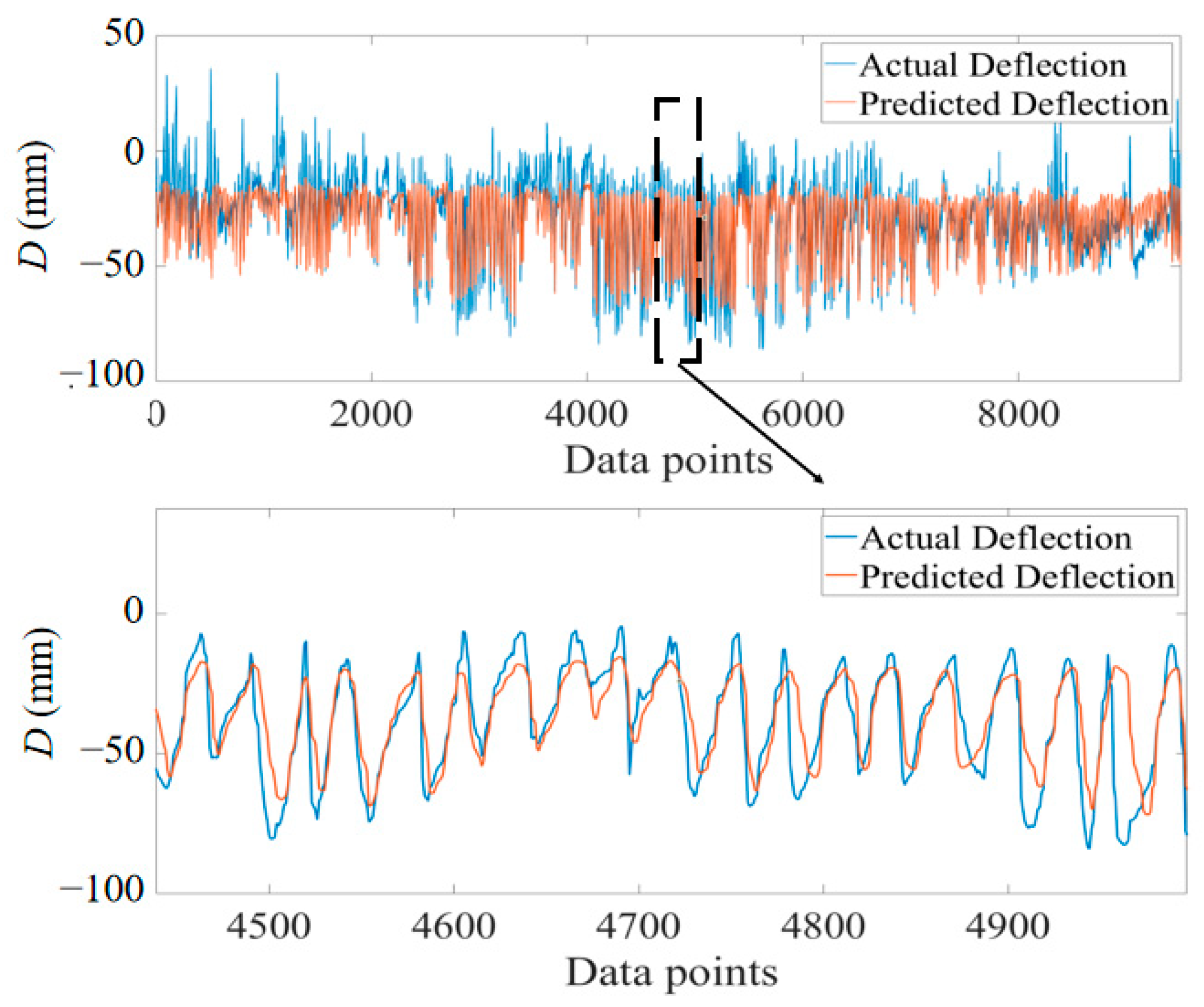
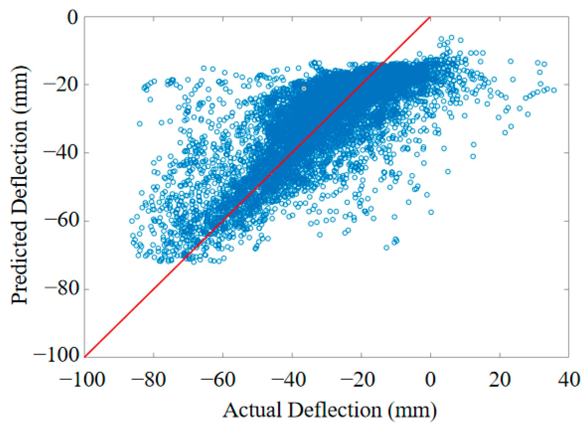
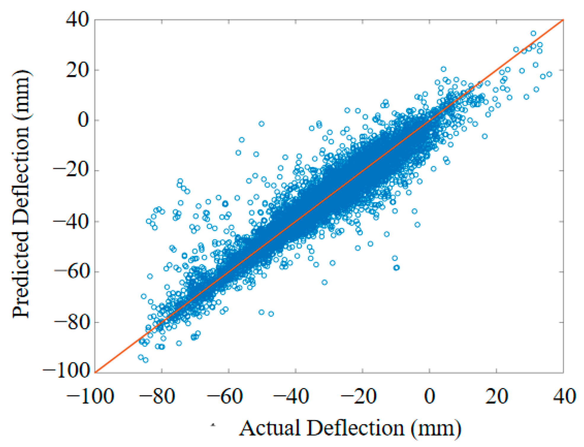
Figure 9 shows the predictive ability of the multiple linear regression model. Figure 10 is the scattered points plot with actual deflection and predicted deflection. The MSE of the test set is 246.73 mm2. The precision of the model established via multiple linear regression analysis is low, and it cannot satisfy the engineering needs. The neural networks with higher fit ability are further used to establish the regression model.

4. Backpropagation Neural Network (BPNN)

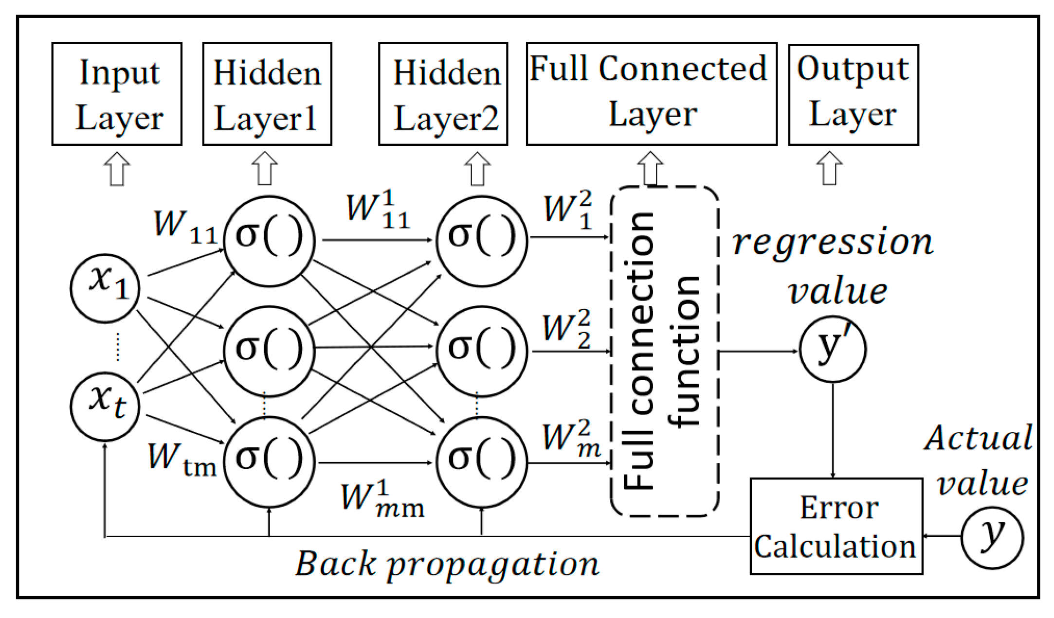
BPNN is a widely used machine learning method with excellent performance in digital regression. A standard BPNN usually consists of an input layer, a hidden layer, and an output layer [23]. As shown in Figure 11, the BPNN has two hidden layers and each layer has m units as an example. In the forward propagation of the BPNN, the data features from 1 to t are firstly input into the input layer. After the calculation using several weight coefficients  W t m , the calculated information is transferred to the hidden layer. After the operation via the activation function σ, the information is processed via the weighting coefficients  W i k 1  in the first hidden layer. Then, the information is further input into the next hidden layer and calculated via the activation function and the weighting coefficients  W k 2  in the second hidden layer. Finally, the fully connected layer integrates the values from the second hidden layer and thereby outputs the predicted regression value y’. In the training process, the parameters of the BPNN are adjusted and optimized through the backpropagation algorithm to improve the precision of the digital regression model.
BPNN is the most classic neural network, and it is used for preliminary exploratory modeling and serves as a benchmark for evaluating other subsequent methods. In this paper, the regression models between the temperature features and the temperature-induced deflection were established via BPNN using the s-type transfer function (logsig function) as the activation function.
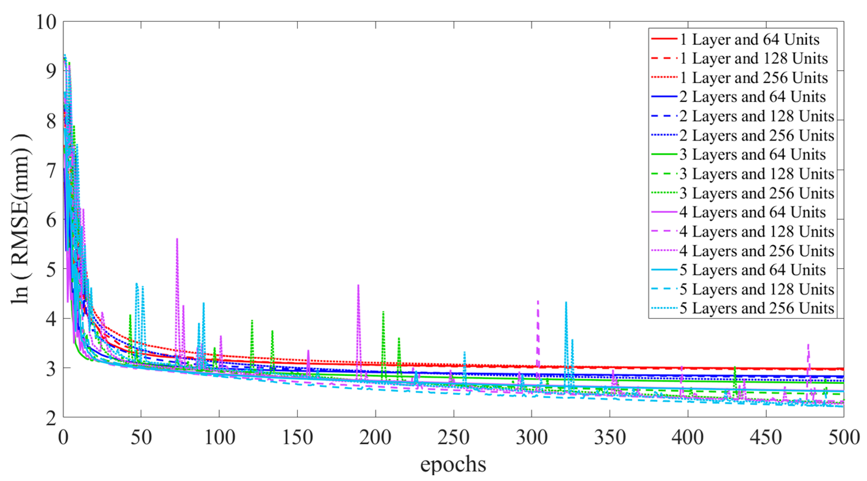
To find the optimal BPNN model parameters, the different BPNN models are trained and tested. The BPNN models have 1 to 5 hidden layers, with each layer having 64, 128, or 256 hidden units. In the training phase, 0.1 is set as the initial learning rate. Figure 12 shows that the root mean square error (RMSE) of the training set changes during the 500 epochs and iterates training of the BPNN model with different architectures. The RMSE is described by Equation (12):
R M S E = n = 1 N ( D n D ¯ ) 2 N
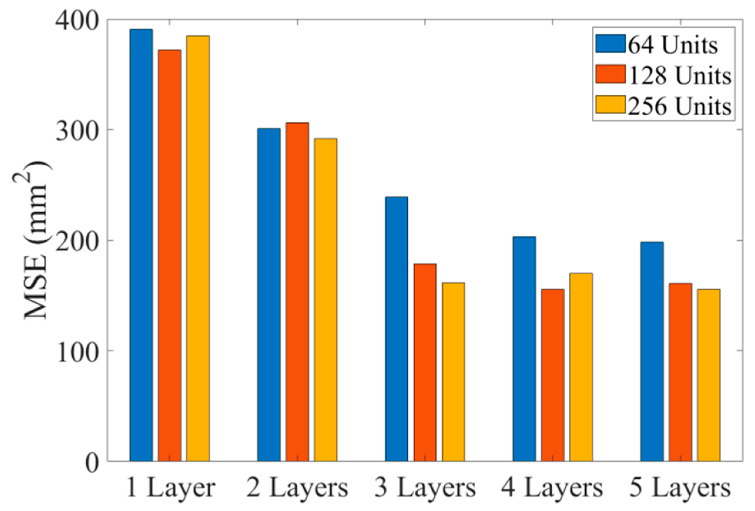
The precision of the trained models was tested. After the 500 epochs iterate training, the mean square errors (MSE) of the test are used evaluate the precision of the different models, as shown in Figure 13. When the number of the hidden layers is one, two, or three, the precision constantly increases. When the hidden layers are increased to four or five layers, the precision almost no longer improves. When the hidden layer is four or five layers, the performances of BPNN with 128 hidden units and 256 hidden units in each hidden layer are not much different. Therefore, under 500 epochs of iteration, the network architecture with five hidden layers and 256 hidden units in each layer is selected to build the regression model. The MSE of the training set and test set obtained via BPNN with different architectures are shown in Table 1.
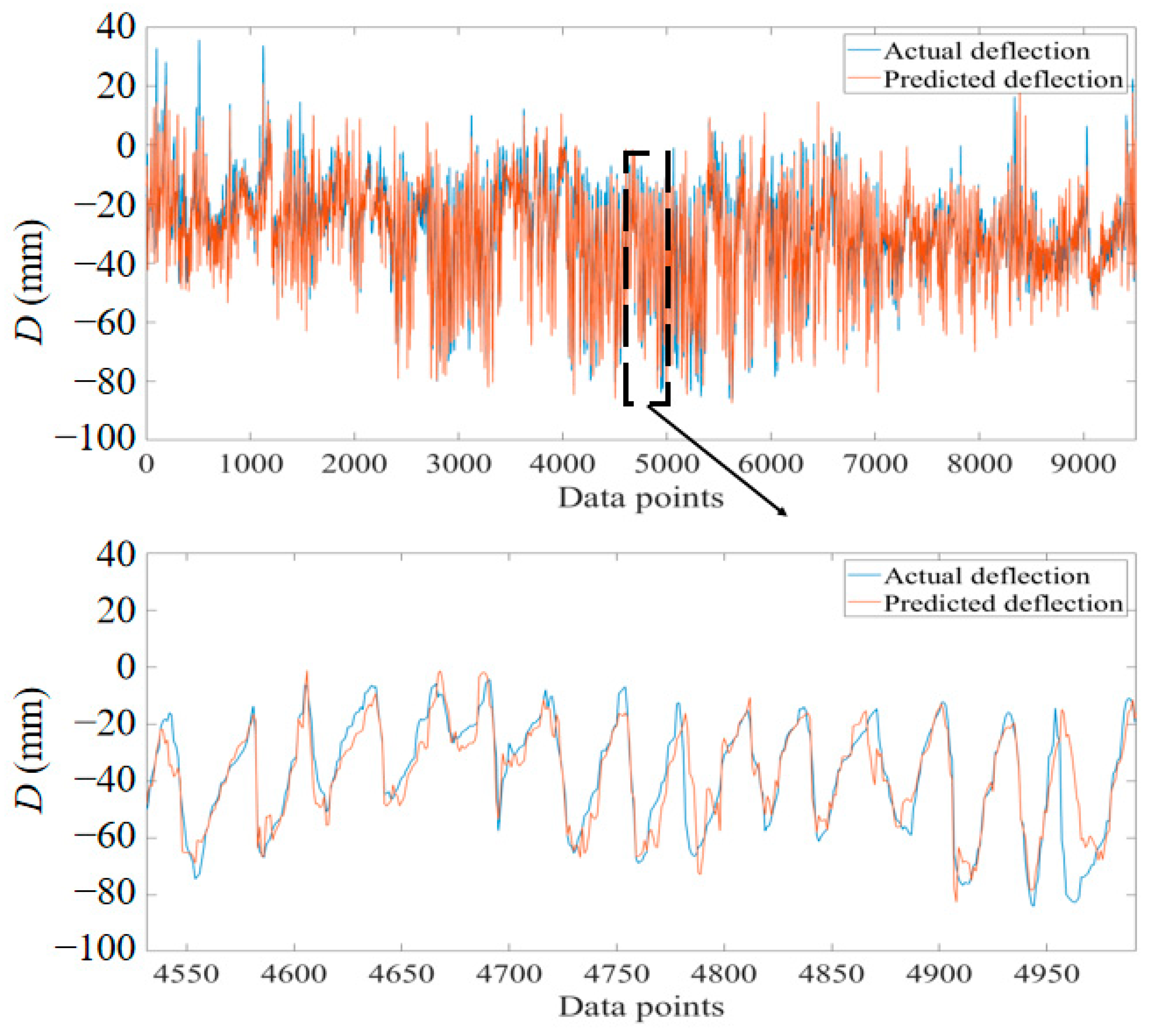
Figure 14 shows the output results of the regression model established via the BPNN with 5 hidden layers and 256 hidden units in each hidden layer. Figure 15 shows the scattered points plot of the actual deflection and predicted deflection. The BPNN regression model is more precise than the MLR model. The MSE of the BPNN model was reduced to 154.09 mm2, but this level of precision is obviously still insufficient.

5. Regression Model Based on Deep Learning

The deep learning network has deeper hidden layers and a more complex computing unit in the hidden layer. It usually has a stronger nonlinear fitting performance than traditional networks, resulting in higher precision in regression modeling [24,25]. Therefore, the deep learning networks are used to further improve the regression performance in this paper.

5.1. Long-Short Term Memory Network (LSTM)

The recurrent neural network (RNN) usually performs well in modeling the time-varying correlation. [26]. Compared with BPNN, RNN considers the information at the current moment and the previous information. Therefore, in this study a time series is used as the input data in the RNN regression model, and then the fitted data at the current moment are output.
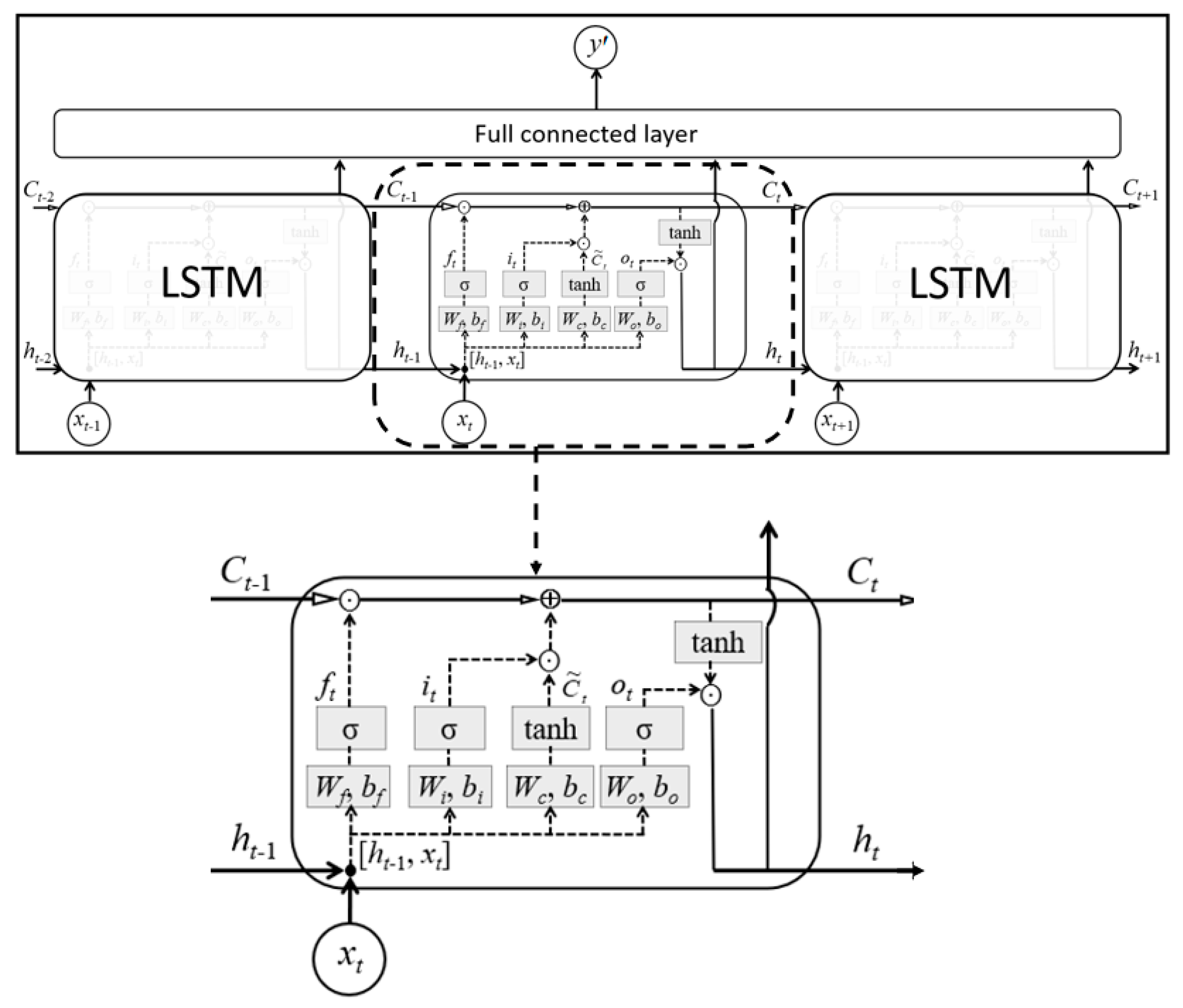
The LSTM network is one type of the improved RNNs. LSTM can more accurately describe temporal nonlinear factors. It can fully mine the longer time series data by its specific gate functions in the unit of the hidden layer [27]. Therefore, the LSTM network satisfies the requirements of explaining the nonlinear time dependence between the different variables. Figure 16 shows the network architecture of LSTM with one LSTM hidden layer.
The data flow in the hidden units and the hidden layers of the LSTM network is more complex than that of the RNN network. For a unit of the LSTM hidden layer, except putting the time series data  { x 1 , x 2 , , x t }  into the model, the input data also include the information  h t 1  transmitted from the LSTM unit at the previous moment, and includes the long-term memory  C t 1  flowing in the cell. Several weights, biases, and activation functions constitute the forget gate, input gate, and output gate. Among the parameters in the LSTM network,  f t  is generated from the forget gate,  i t  and  C ˜ t  are generated from the input gate, and  O t  is generated from the output gate. The gate parameters are calculated by Equations (13) to (16):
f t = σ ( W f [ h t 1 , x t ] + b f )
i t = σ ( W i [ h t 1 , x t ] + b i )
C ˜ t = tanh ( W C [ h t 1 , x t ] + b C )
O t = σ ( W O [ h t 1 , x t ] + b O )
where  W C W f W i W O  are weight coefficients;  b C b f b i b O  are biases.
Due to the existence of the forget gate, the long-term information transmitted by the previous cell is only partially retained. The product of the parameters  f t  and  C t 1 , and the product of the parameters  i t  and  C ˜ t , determine the update of information. Therefore, the current  C t  can be updated to achieve better computational results. The parameter  C t  is described by Equation (17):
C t = f t C t - 1 + i t C ˜ t
h t  is not only the output value of the network at the current moment, but also the information passed to the next cell.  h t  is described by Equation (18):
h t = O t tanh ( C t )

5.2. Nested Long Short-Term Memory Network (NLSTM)

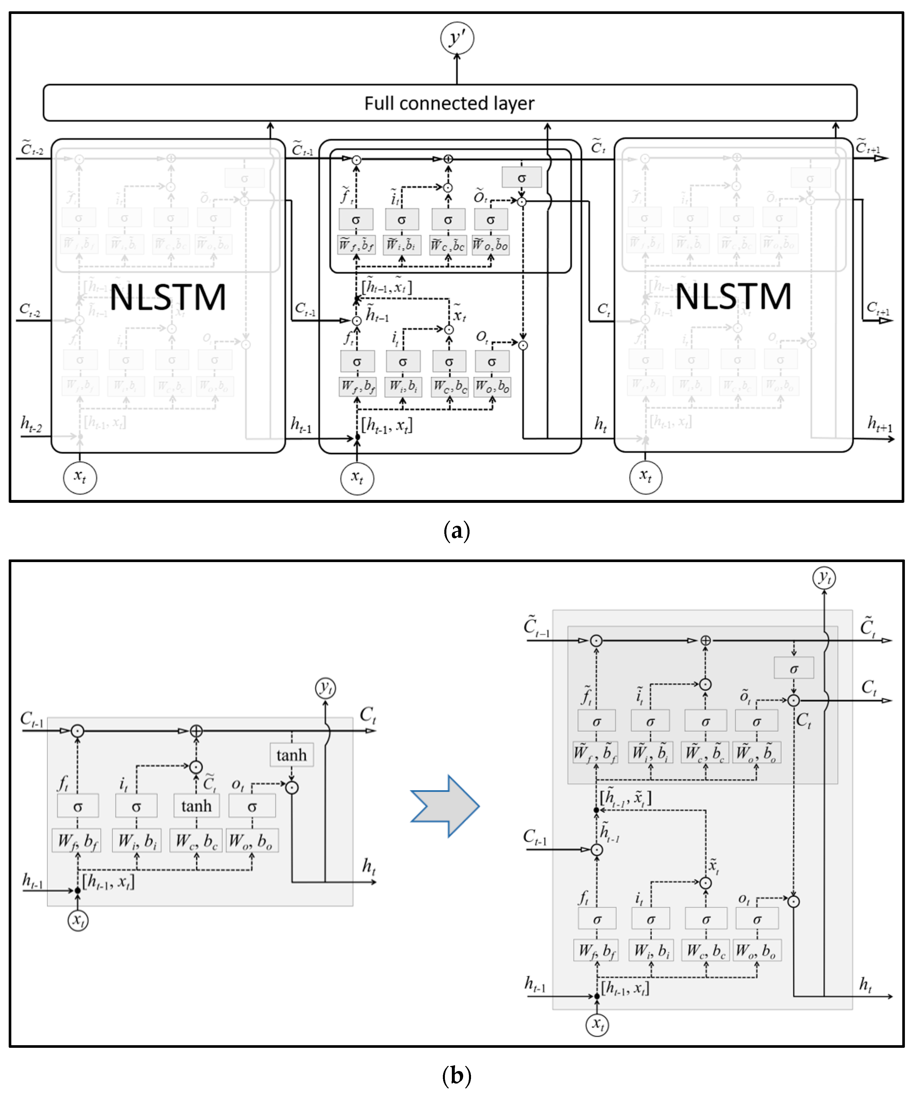
NLSTM is an optimized LSTM architecture jointly proposed by Carnegie Mellon University and the University of Montreal. NLSTM can express a higher nonlinear relationship than traditional LSTM by the more refined calculation in the hidden units.
As shown in Figure 17, the NLSTM unit has a deeper architecture than the LSTM unit. The parameters in NLSTM can be described by Equations (19) to (29):
f t = σ ( W f [ h t 1 , x t ] + b f )
i t = σ ( W i [ h t 1 , x t ] + b i )
O t = σ ( W O [ h t 1 , x t ] + b O )
x ˜ t = i t × σ ( W c [ h t 1 , x t ] + b c )
h ˜ t 1 = f t C t 1
f ˜ t = σ ( W ˜ f [ h ˜ t 1 , x ˜ t ] + b ˜ f )
i ˜ t = σ ( W ˜ i [ h ˜ t 1 , x t ˜ ] + b ˜ i )
O ˜ t = σ ( W ˜ O [ h ˜ t 1 , x ˜ ] + b ˜ O )
C ˜ t = f ˜ t C ˜ t 1 + i ˜ t σ ( W ˜ C [ h ˜ t 1 , x ˜ t ] + b ˜ C )
C t = O ˜ t σ ( C ˜ t )
h t = O t C t
where  W C W f W i W O  are weight coefficients;  b C b f b i b O  are biases.

5.3. Optimized Architecture for NLSTM Network

The NLSTM network is established based on MATLAB. It also establishes the regression relationship between the temperature features changing over time and Dt.
Because the dataset was processed via the PCA-LGBM algorithm, the data do not need to be normalized. In the NLSTM network, the training datasets are still X1 and D1. The NLSTM network and its parameters were dissected as shown in Figure 17. During the training phase, the parameters are continuously adjusted via backpropagation.
After the NLSTM network undergoes the preset iterative epochs of optimization training, a regression model is obtained. To test the performance of this regression model, the test set X2 is used as the input data, and the predicted values calculated by the model are compared with the actual D2.
Due to the limited capacity of the NLSTM with only one hidden layer for handling engineering problems, the neural networks must be organized into an optimized architecture [28,29]. It is necessary to find the best network architecture for NLSTM to ensure accuracy.
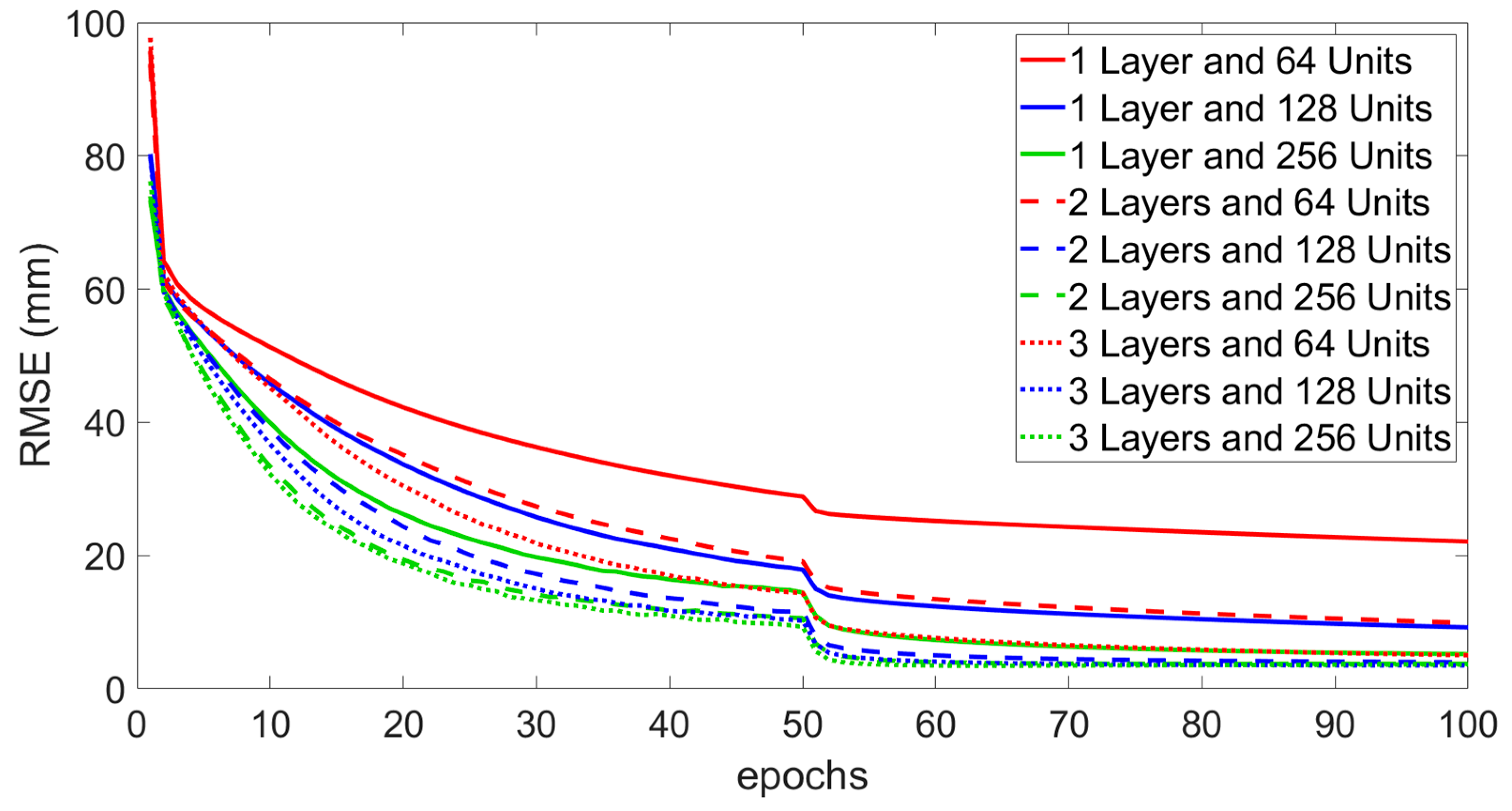
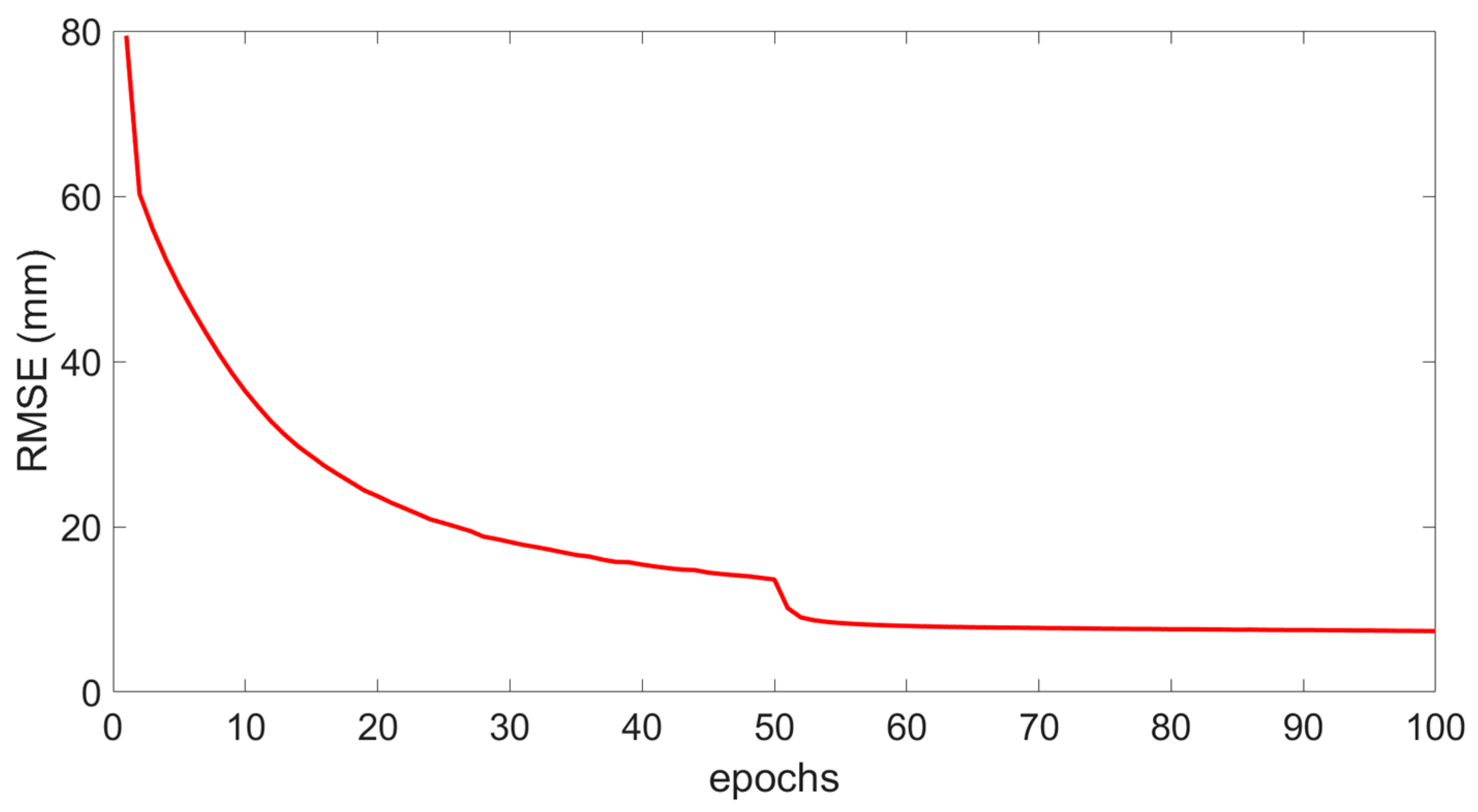
Considering the data scale and the computing power of our device, this paper sets the batch size as 32, and uses the Adam optimizer in backward propagation. The training process has 100 iterative epochs. To speed up the convergence speed, the initial learning rate is set to 0.001, and it will reduce to 0.0002 after 50 epochs to ensure the convergence of the NLSTM network.
The datasets X1 and D1 are utilized to, respectively, train NLSTM networks with single, double, and triple hidden layers. The units in each hidden layer change from 64 hidden units to 128 hidden units to 256 hidden units. Figure 18 shows the root mean square error (RMSE) of the training set changes during 100 epochs of nine NLSTM networks with different architectures.
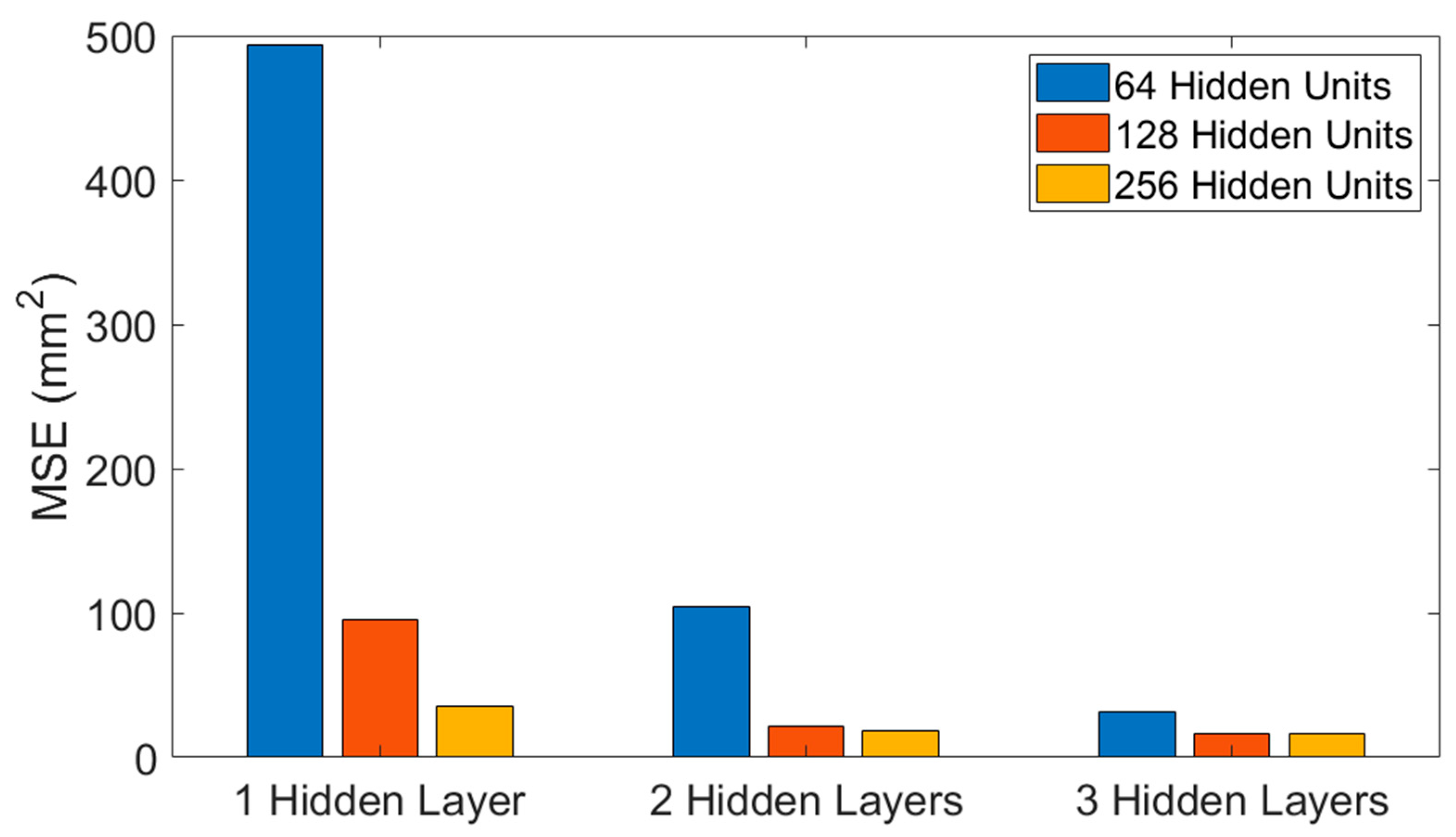
The test sets X2 and D2 were applied to test the precision of the nine models after the training. Figure 19 shows the mean square error of the predicted results of the nine NLSTM networks with different architectures. This picture is used to roughly observe the situation and more detailed results are provided in Table 2.
The MSE of the training set and test set for the NLSTM networks with different architectures are shown in Table 2. Benefiting from the excellent temperature feature extracted via the PCA-LGBM algorithm and reasonable hyperparameter selection, even the NLSTM network with 1 hidden layer and 64 hidden units does not show a significant difference between the training results and testing results. This proves that there is no overfitting or other singular phenomenon when the trained model is used for the practical test.
The root mean square error of the NLSTM network with n hidden layers and m hidden units after 100 epochs of training is represented as  R n m . The root mean square errors of different NLSTM networks are sorted from largest to smallest as shown below:
R 1 64 > R 2 64 > R 1 128 > R 1 256 > R 3 64 > R 2 128 > R 2 256 > R 3 128 > R 3 256
In considering the training effect alone, it can be seen that all nine networks are converged. The root mean square error of the NLSTM network with a single hidden layer and 64 hidden units is larger than other networks. Of course, an evaluation of the ability of a neural network must also consider the test effect.
For the test results, a similar conclusion can also be proved from the mean square errors of the nine NLSTM networks in Figure 19 and Table 2. The root mean square error reduces the increases in the number of hidden layers and hidden units in the NLSTM network. The mean square error of some NLSTM networks are very similar. This illustrates that there is no significant difference in fitting ability between the NLSTM networks, and the networks should be further selected by considering the computational efficiency.
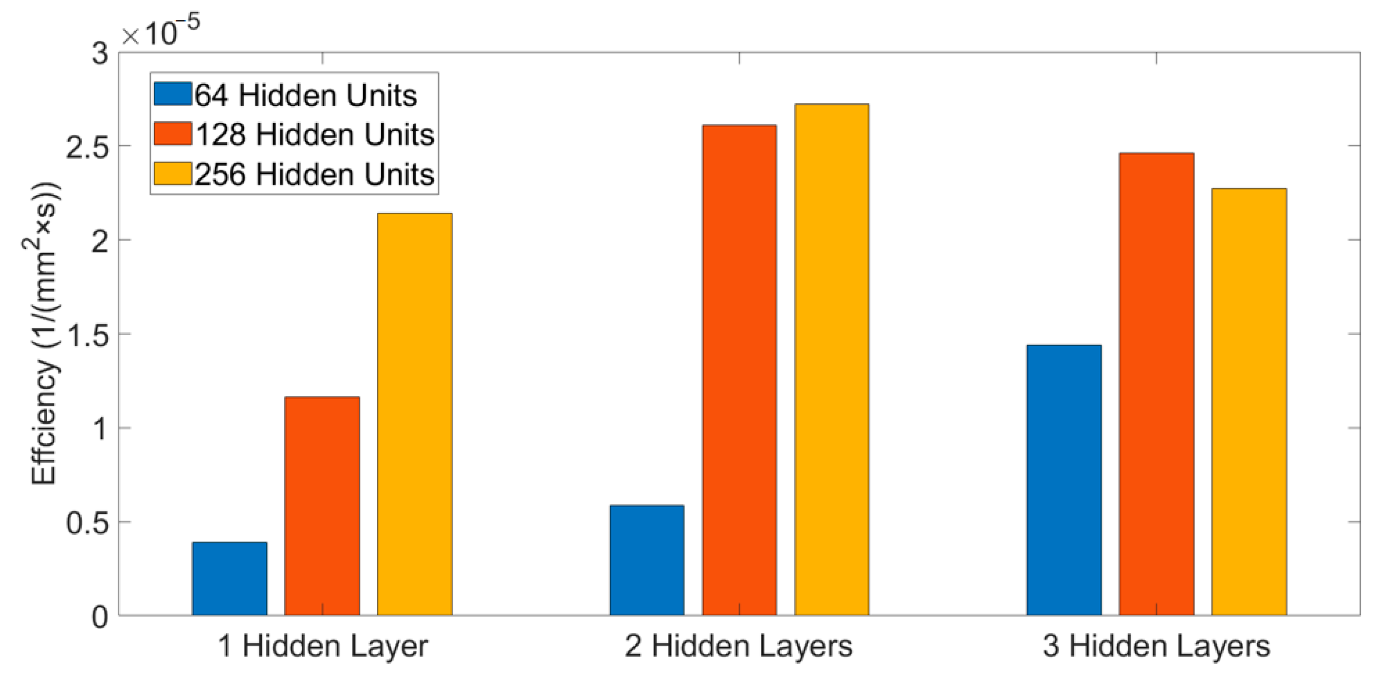
We can further evaluate the performances and efficiencies of the NLSTM networks with different architectures through the test precision and training time. After 100 epochs of iterative training, for the nine different NLSTM networks, the training time and the mean square error of the test set make up the two arrays as follows:
{ t 1 64 ,   t 1 128 ,   t 1 256 ,   t 2 64 ,   t 2 128 ,   t 2 256 ,   t 3 64 ,   t 3 128 ,   t 3 256 }
{ M 1 64 ,   M 1 128 ,   M 1 256 ,   M 2 64 ,   M 2 128 ,   M 2 256 ,   M 3 64 ,   M 3 128 ,   M 3 256 }
where  t n m  represents the time cost in 100 epochs of training for the NLSTM network with n hidden layers and each hidden layer with m hidden units.  M n m  represents the mean square error of the test set of the NLSTM network with n hidden layers and each layer with m hidden units.  η n m  is the product of the corresponding values in the two arrays and is used as the indicator to evaluate the efficiency of NLSTM networks. The parameter  η n m  is described by Equation (30):
η n m = 1 t n m × 1 M n m
Figure 20 shows the comparison of the  η n m  of the different NLSTM networks. The NLSTM networks with 64 hidden units per hidden layer are the most inefficient. The NLSTM network with 2 hidden layers and each layer with 256 hidden units is the optimal choice.
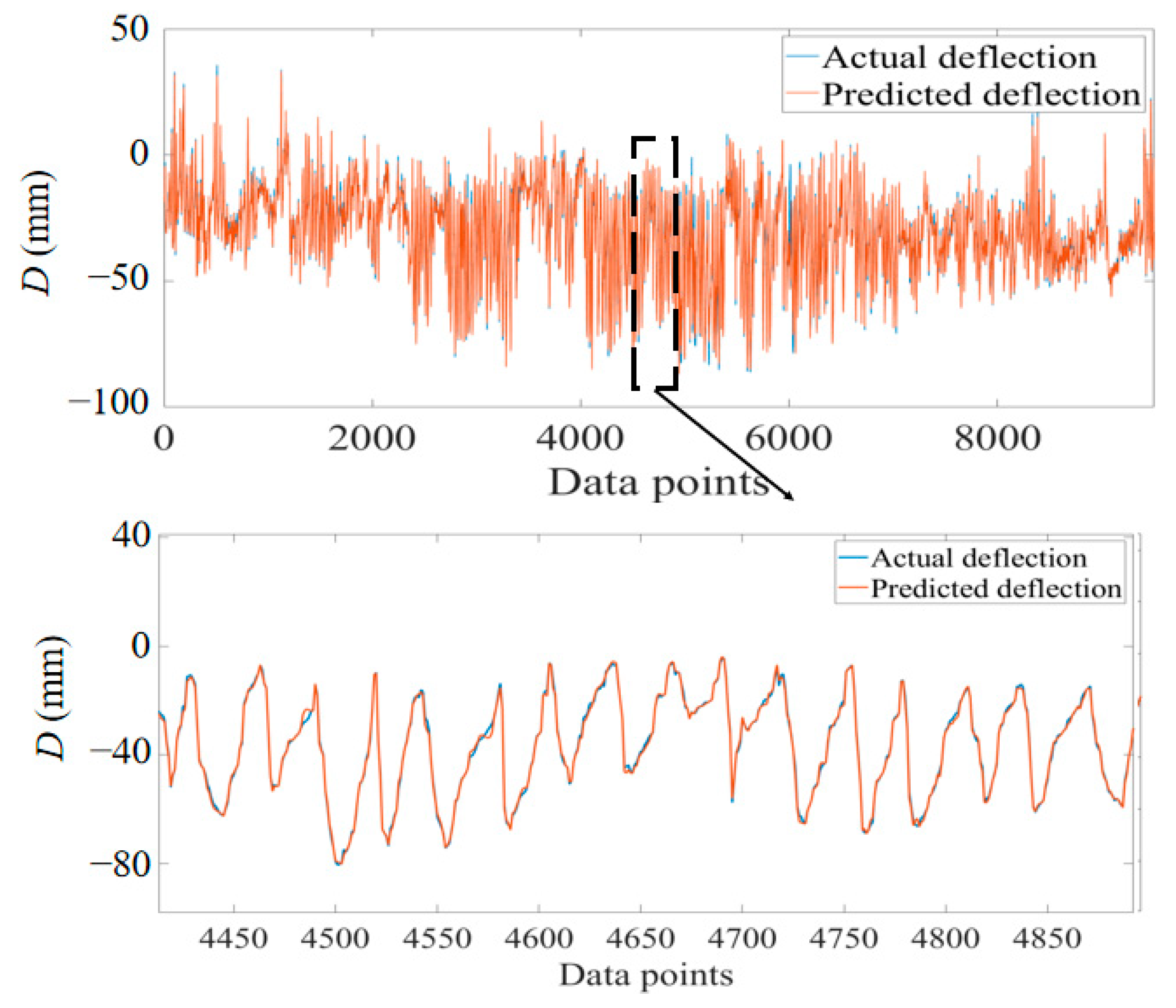
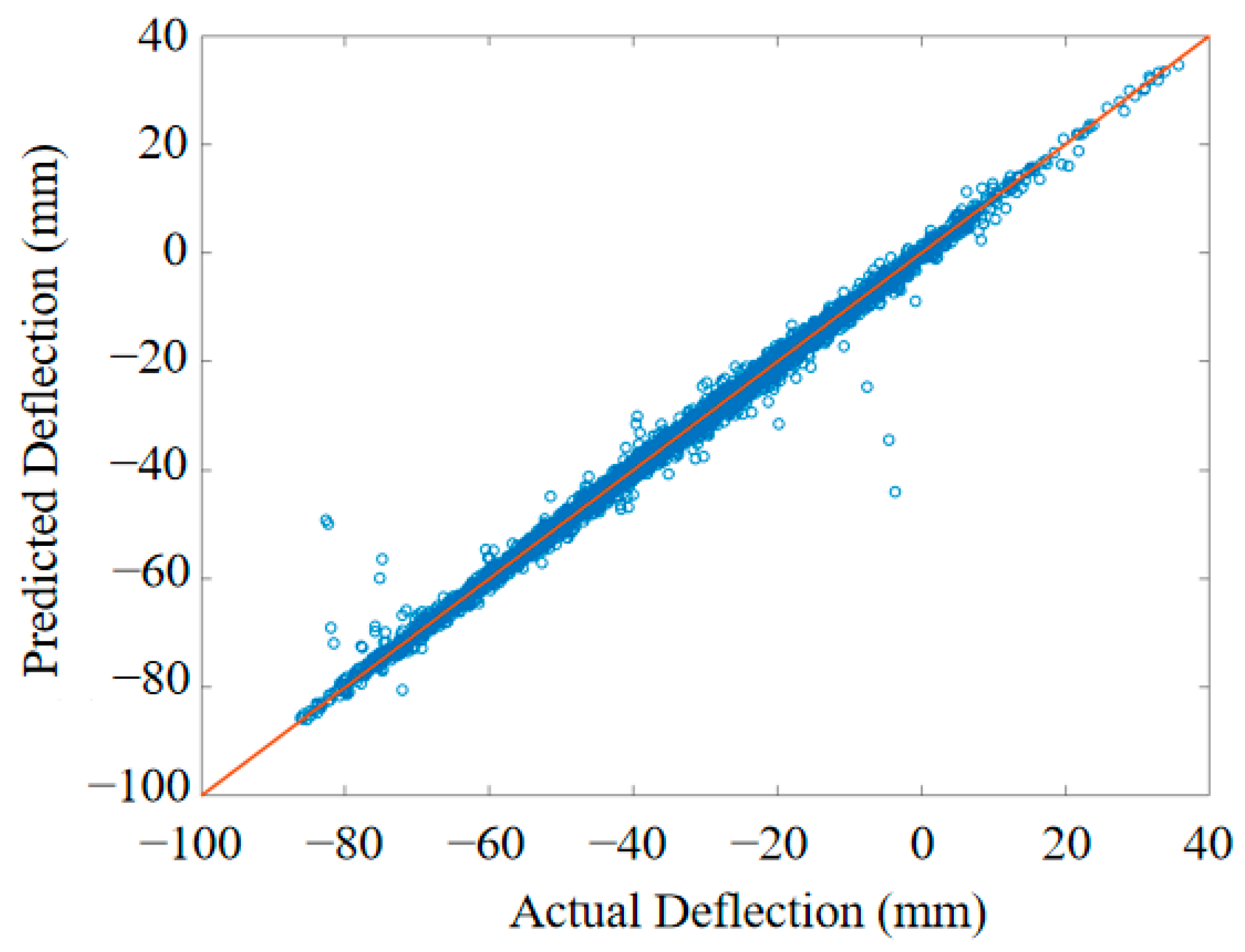
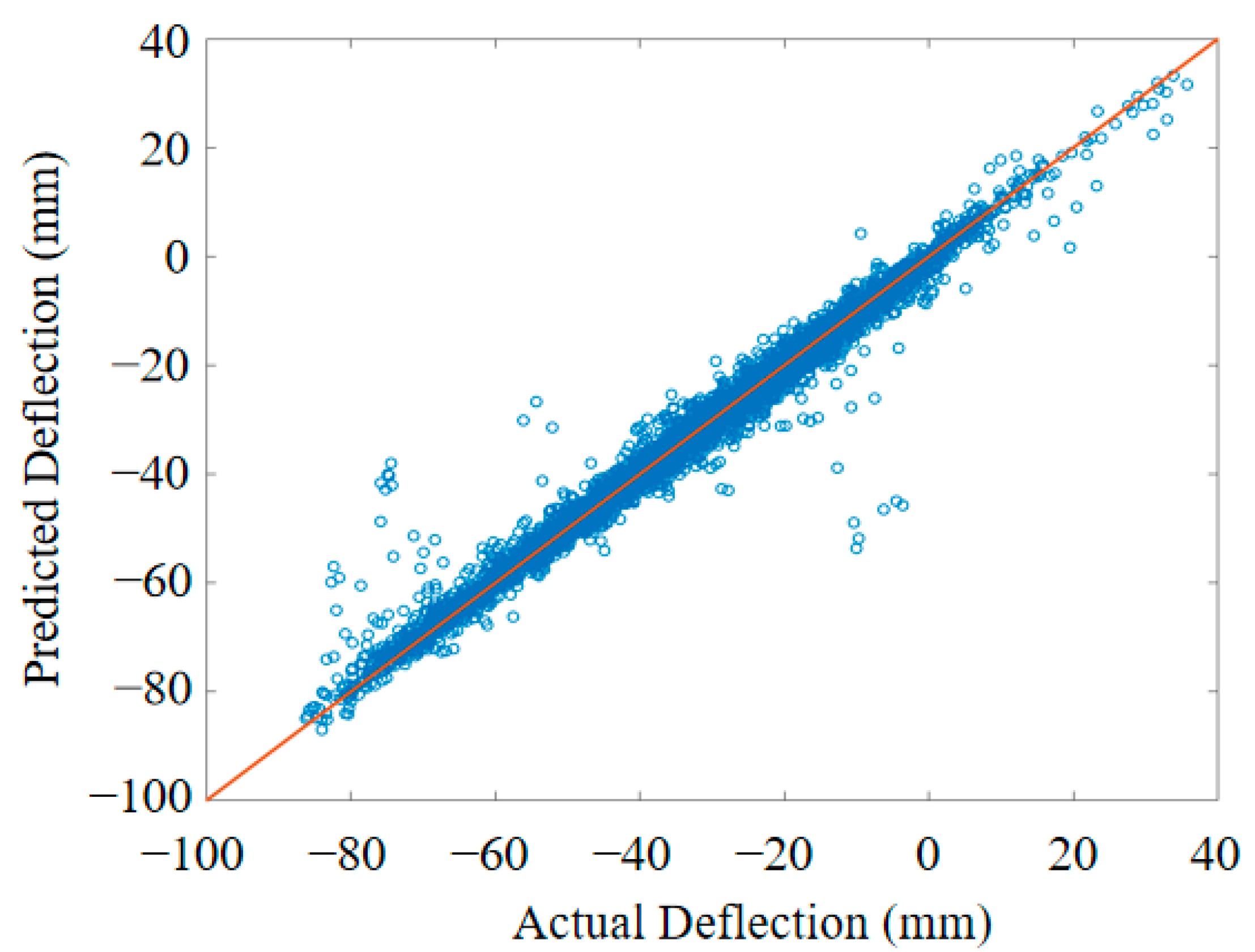
Figure 21 shows the output results of the regression model established by the NLSTM network which has 2 hidden layers and 256 hidden units in each hidden layer. Figure 22 shows the scattered plot of the actual deflection and the predicted deflection. The mean square error of the test set is 18.57 mm2 and it is more accurate than the BPNN regression model.
To demonstrate that the NLSTM unit has better performance than the classical LSTM unit, the LSTM regression model is also established with 2 hidden layers and 256 hidden units for the test set. Figure 23 shows the RMSE changes during 100 epochs of the training set for the LSTM network. The network, which is established by the classic LSTM, still converges during the training phase.
For this LSTM model, the mean square error of the test set is 66.95 mm2. Figure 24 shows the output result of the LSTM regression model. Figure 25 shows the scattered plot with actual deflection and predicted deflection. Obviously, the precision of NLSTM is superior to that of LSTM. The results of different models are further compared and discussed in the next section.

6. Evaluation of Several Models

Three indicators were selected to assess the accuracy of different models more comprehensively. These three indicators are, respectively, the MSE, which is described by Equation (11), the Maximum Absolute Error (MAXAE), described by Equation (31), and the Mean Absolute Error (MAE), described by Equation (32). The MAE evaluates the overall error; the MSE evaluates the output stability; and the MAXAE evaluates the extreme value of error.
M A X A E = max | D n D n |
M A E = 1 n | D n D n |
The above error indicators were, respectively, tested using the regression values from the MLR, BPNN, LSTM, and NLSTM regression models which were trained using the datasets from the combined PCA-LGBM. To demonstrate the applicability and effectiveness of the four extracted temperature features of the combined PCA-LGBM algorithm, the same training and testing procedures were performed by randomly selecting four temperature features, and the above error indicators of the selected methods of the randomly selected four temperature features are calculated again. The relevant calculation results are shown in Table 3.
The discussion of the several calculation results is as follows:
When the MLR model is used for fitting with features via PCA-LGBM, the MAE of the model is 18.26 mm. The MSE is 246.73 mm2, which is approximately 16.5 times the MAE, showing poor accuracy and stability. The MAXAE of the model is 61.80 mm.
When using BPNN with 5 hidden layers and 256 hidden units per layer to establish a regression model for fitting with features via PCA-LGBM, the model MAE is 12.63 mm. The MSE is 154.09 mm2, which is approximately 8.5 times the MAE. The accuracy and stability of the model have improved to a certain extent. The MAXAE of the model is reduced to 50.44 mm.
When the regression model is established using the LSTM network with 2 hidden layers and 256 hidden units in each hidden layer, for the fitting with features via PCA-LGBM, the MAE is reduced to 8.06 mm. The MSE is only 66.95 mm2, approximately twice the MAE. The model accuracy and stability were significantly improved. The MAXAE was reduced to 33.16 mm.
When the regression model is established using the NLSTM network with 2 hidden layers and 256 hidden units in each hidden layer, for the fitting with features via PCA-LGBM, MAE is reduced to 4.76 mm. The MSE is only 18.57 mm2, approximately twice the MAE. The model accuracy and stability were significantly improved. The MAXAE was reduced to 27.37 mm.
When using the randomly selected features, the errors of the calculation results obtained using the selected methods are all too large for engineering application. Obviously, if the extracted datasets obtained using the PCA-LGBM intelligent algorithm presented in this paper are not used, the reliable model cannot be established even by using the advanced fitting tools.
Therefore, the regression model established using the NLSTM network has superior stability and accuracy with appropriate hyperparameters and reasonable datasets extracted via PCA-LGBM. The model demonstrates a very high precision and can, therefore, provide a very valuable control group for bridge maintenance. Abnormal bridge states can be detected as early as possible; therefore, the model will play a huge role in the assessment of bridge states.
This article is based on the data of a cable-stayed bridge in service; however, the modeling approach and data extraction algorithm can generally be applied to other cable-stayed bridges. Therefore, the relevant methods and schemes in this article have relevant significance for the maintenance of other cable-stayed bridges in service. At the same time, we are committed to continuously developing more advanced methods in the future.

7. Conclusions and Prospect

The relevant conclusions of this article are as follows:
(1)
After verification, for the structural health monitoring data, the main temperature features extracted from the complex temperature field via the PCA-LGBM algorithm have a reliable generalization. It is impossible to build a precise model using the randomly selected features. Thus, the algorithm plays an important role in intelligent regression analysis.
(2)
The architecture of the NLSTM network should be optimized. On the one hand, if there are too few hidden layers and units, the requirements of prediction accuracy and generalization performance will be difficult to satisfy. On the other hand, if the layers and units are too numerous, a substantial computational cost will be incurred with little improvement in model accuracy. In this regard, the NLSTM network with 2 hidden layers, each with 256 hidden units, is the best choice.
(3)
The deep learning-based NLSTM network has higher stability and accuracy in regression analysis compared with traditional MLR analysis and machine learning-based BPNN. Its MAE is only one-twelfth of that of the MLR model, and only one-fifth of that of the BPNN regression model. The ratio of MSE to MAE (MSE/MAE) is only one-seventh of that of the MLR model, and only one-fourth of that of the BPNN regression model, illustrating the strong stability of the proposed NLSTM model. Similarly, the calculation results of NLSTM are better than those of classical LSTM, indicating that using NLSTM to build the regression model of the temperature-induced deflection for cable-stayed bridges is preferred.
The significance and research prospects of this article are as follows:
By using NLSTM and the features extracted via PCA-LGBM, the model can reach a very high precision, thus providing a very valuable control group for bridge maintenance. Therefore, the abnormal state of the bridge can be detected as early as possible. Of course, this paper only provides one fitting tool, and using the regression value of this tool to detect abnormal states still requires the further work consisting of numerical simulations, experiments, and various mathematical tools. This research will continue in the future.

Author Contributions

Conceptualization, Z.W. and Y.D.; funding acquisition, Z.W. and S.S.; investigation, Z.W.; methodology, J.G. and Y.D.; resources, Y.D. and Z.X.; software, J.G.; validation, Z.Y.; writing—original draft, J.G.; writing—review and editing, Y.D. All authors have read and agreed to the published version of the manuscript.

Funding

This research was partially supported by the National Key Research and Development Program (2019YFB1600702), the Shenzhen Technology Research Project (CJGJZD20210408092601005), and the Program of National Natural Science Foundation of China (51978154).

Institutional Review Board Statement

Not applicable.

Informed Consent Statement

Not applicable.

Data Availability Statement

Not applicable.

Acknowledgments

The authors would like to thank the editors and the anonymous reviewers for their valuable comments on the content and the presentation of this article.

Conflicts of Interest

The authors declare no conflict of interest.

References

  1. Sun, L.; Shang, Z.; Xia, Y.; Bhowmick, S.; Nagarajaiah, S. Review of Bridge Structural Health Monitoring Aided by Big Data and Artificial Intelligence: From Condition Assessment to Damage Detection. J. Struct. Eng. 2020, 146, 04020073. [Google Scholar] [CrossRef]
  2. Miyamoto, A.; Motoshita, M. A Study on the intelligent bridge with an advanced monitoring system and smart control techniques. Smart Struct. Syst. 2017, 19, 587–599. [Google Scholar]
  3. Xia, G.P. Parametric Study of Cable Deflection and Gravity Stiffness of Cable-Stayed Suspension Bridge. Appl. Mech. Mater. 2014, 488–489, 445–448. [Google Scholar] [CrossRef]
  4. Zhao, H.W.; Ding, Y.L.; Nagarajaiah, S.; Li, A.Q. Behavior Analysis and Early Warning of Girder Deflections of a Steel-Truss Arch Railway Bridge under the Effects of Temperature and Trains: Case Study. J. Bridge Eng. 2019, 24, 05018013. [Google Scholar] [CrossRef]
  5. Ding, Y.; Wang, G.; Zhou, G.; Li, A. Life-cycle simulation method of temperature field of steel box girder for Runyang cable-stayed bridge based on field monitoring data. China Civ. Eng. J. 2013, 46, 129–136. [Google Scholar]
  6. Xu, X.; Xu, C.B.; Zhang, Y.; Wang, H.L. Preliminary Study on the Loss Laws of Bearing Capacity of Tunnel Structure. Symmetry 2021, 13, 1951. [Google Scholar] [CrossRef]
  7. Zhou, Y.; Sun, L.M.; Fu, Z.H.; Jiang, Z.; Ren, P.J. General formulas for estimating temperature-induced mid-span vertical displacement of cable-stayed bridges. Eng. Struct. 2020, 221, 111012. [Google Scholar] [CrossRef]
  8. Zhou, Y.; Sun, L.M.; Fu, Z.H.; Jiang, Z. Study on temperature sensitivity coefficients of mid-span vertical displacement of cable-stayed bridges. Eng. Mech. 2020, 37, 148–154. (In Chinese) [Google Scholar]
  9. Zhou, Y.; Sun, L.M. Insights into temperature effects on structural deformation of a cable-stayed bridge based on structural health monitoring. Struct. Health Monit. 2019, 18, 778–791. [Google Scholar] [CrossRef]
  10. Wang, M.; Ding, Y.; Wan, C.; Zhao, H. Big data platform for health monitoring systems of multiple bridges. Struct. Monit. Maint. 2020, 7, 345. [Google Scholar]
  11. Chengfeng, T.; Zejia, L.; Ge, Z. Processing technique and application of big data oriented to long-term bridge health monitoring. J. Exp. Mech. 2017, 32, 652–663. [Google Scholar]
  12. Cai, G.W.; Mahadevan, S. Big Data Analytics in Uncertainty Quantification: Application to Structural Diagnosis and Prognosis. ASCE-ASME J. Risk Uncertain. Eng. Syst. Part A Civ. Eng. 2018, 4, 04018003. [Google Scholar] [CrossRef]
  13. Huang, H.B.; Yi, T.H.; Li, H.N. Canonical correlation analysis based fault diagnosis method for structural monitoring sensor networks. Smart Struct. Syst. 2016, 17, 1031–1053. [Google Scholar] [CrossRef]
  14. Punmiya, R.; Choe, S. Energy theft detection using gradient boosting theft detector with feature engineering-based preprocessing. IEEE Trans. Smart Grid 2019, 10, 2326–2329. [Google Scholar] [CrossRef]
  15. Wang, L.; Zeng, Y.; Chen, T. Back propagation neural network with adaptive differential evolution algorithm for time series forecasting. Expert Syst. Appl. 2015, 42, 855–863. [Google Scholar] [CrossRef]
  16. Singh, A.; Kushwaha, S.; Alarfaj, M.; Singh, M. Comprehensive overview of backpropagation algorithm for digital image denoising. Electronics 2022, 11, 1590. [Google Scholar] [CrossRef]
  17. Ma, X.; Zhong, H.; Li, Y.; Ma, J.; Cui, Z.; Wang, Y. Forecasting transportation network speed using deep capsule networks with nested LSTM models. IEEE Trans. Intell. Transp. Syst. 2020, 22, 4813–4824. [Google Scholar] [CrossRef] [Green Version]
  18. Smagulova, K.; James, A.P. A survey on LSTM memristive neural network architectures and applications. Eur. Phys. J. Spec. Top. 2019, 228, 2313–2324. [Google Scholar] [CrossRef]
  19. Liu, H.; Ding, Y.L.; Zhao, H.W.; Wang, M.Y.; Geng, F.F. Deep learning-based recovery method for missing structural temperature data using LSTM network. Struct. Monit. Maint. 2020, 7, 109–124. [Google Scholar]
  20. Erichson, N.B.; Zheng, P.; Manohar, K.; Brunton, S.L.; Kutz, J.N.; Aravkin, A.Y. Sparse Principal Component Analysis via Variable Projection. SIAM J. Appl. Math. 2018, 80, 977–1002. [Google Scholar] [CrossRef]
  21. Ju, Y.; Sun, G.; Chen, Q.; Zhang, M.; Zhu, H.; Rehman, M.U. A Model Combining Convolutional Neural Network and LightGBM Algorithm for Ultra-short-term Wind Power Forecasting. IEEE Access 2019, 7, 28309–28318. [Google Scholar] [CrossRef]
  22. Yue, Z.X.; Ding, Y.L.; Zhao, H.W.; Wang, Z.W. Mechanics-Guided optimization of an LSTM network for Real-Time mod-eling of Temperature-Induced deflection of a Cable-Stayed bridge. Eng. Struct. 2022, 252, 113619. [Google Scholar] [CrossRef]
  23. Liu, Y.; Jing, W.; Xu, L. Cascading model based back propagation neural network in enabling precise classification. In Proceedings of the 2016 12th Interna-tional Conference on Natural Computation, Fuzzy Systems and Knowledge Discovery (ICNC-FSKD), Changsha, China, 13–15 August 2016; pp. 7–11. [Google Scholar]
  24. Williams, R.J.; Zipser, D. A Learning Algorithm for Continually Running Fully Recurrent Neural Networks. Neural Comput. 1989, 1, 270–280. [Google Scholar] [CrossRef]
  25. Yue, Z.X.; Ding, Y.L.; Zhao, H.W.; Wang, Z.W. Case Study of Deep Learning Model of Temperature-Induced Deflection of a Cable-Stayed Bridge Driven by Data Knowledge. Symmetry 2021, 13, 2293. [Google Scholar] [CrossRef]
  26. Hang, R.L.; Liu, Q.S.; Hong, D.F.; Ghamisi, P. Cascaded Recurrent Neural Networks for Hyperspectral Image Classification. IEEE Trans. Geosci. Remote Sens. 2019, 57, 5384–5394. [Google Scholar] [CrossRef] [Green Version]
  27. Zhang, Y.Z.; Xiong, R.; He, H.W.; Pecht, M.G. Long-short-Term Memory Recurrent Neural Network for Remaining Useful Life Prediction of Lithium-Ion Batteries. IEEE Trans. Veh. Technol. 2018, 67, 5695–5705. [Google Scholar] [CrossRef]
  28. Yu, Y.; Si, X.S.; Hu, C.H.; Zhang, J.X. A Review of Recurrent Neural Networks: LSTM Cells and Network Architectures. Neural Comput. 2019, 31, 1235–1270. [Google Scholar] [CrossRef]
  29. Nakisa, B.; Rastgoo, M.N.; Rakotonirainy, A.; Maire, F.; Chandran, V. Long-short Term Memory Hyperparameter Optimization for a Neural Network Based Emotion Recognition Framework. IEEE Access 2018, 6, 49325–49338. [Google Scholar] [CrossRef]
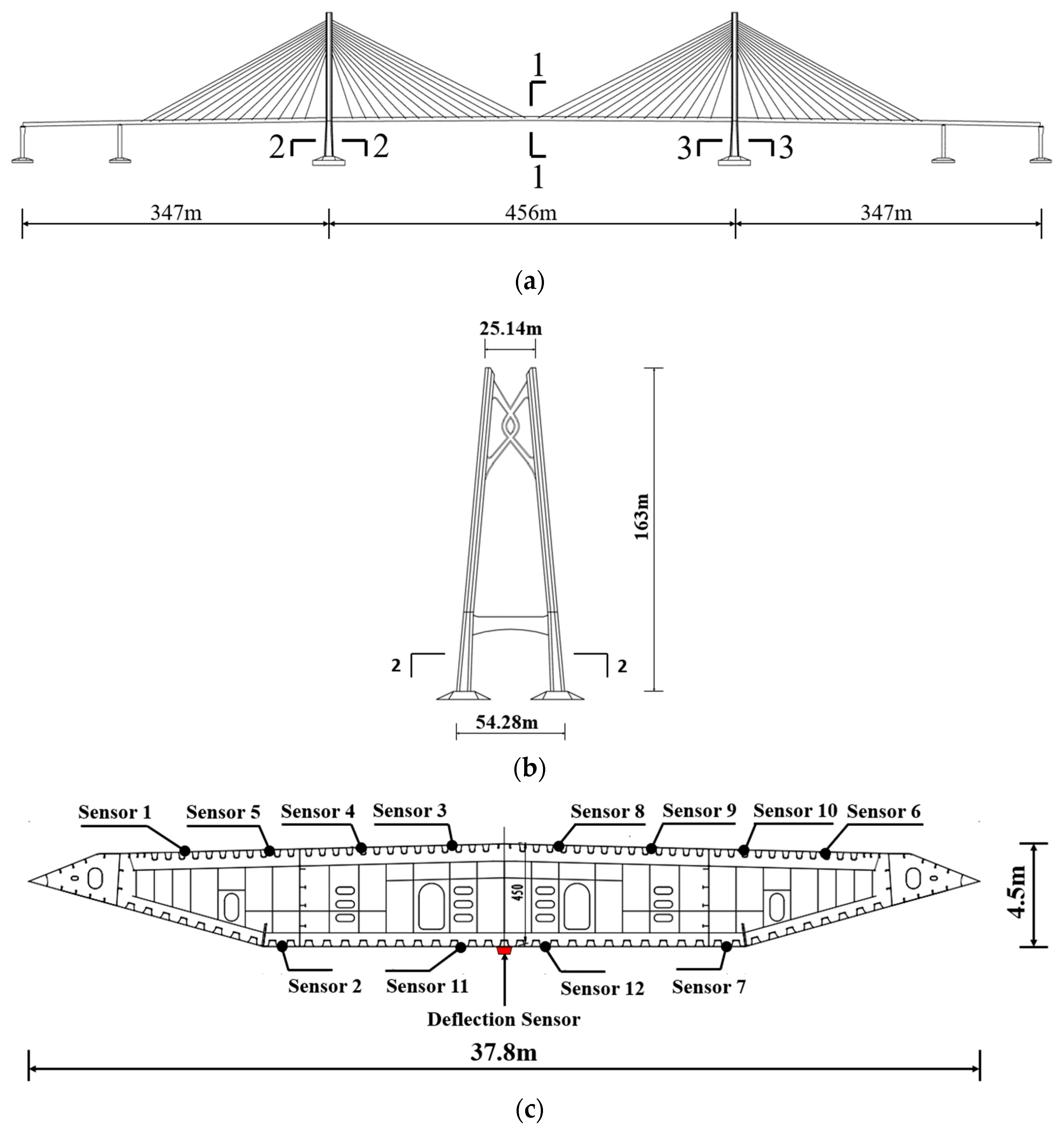
Figure 1. Positions of the temperature sensors installed on the bridge. (a) Elevation of the cable-stayed bridge, (b) Bridge tower, (c) Section 1-1, (d) Section 2-2, (e) Section 3-3.
Sustainability 15 09623 g001aSustainability 15 09623 g001b
Figure 2. Time–history curves of the original deflection and the temperature-induced deflection on 4 January 2020.
Sustainability 15 09623 g002
Figure 3. Time–history curve of the temperature-induced deflection.
Sustainability 15 09623 g003
Figure 4. Time–history curves of the temperature measured via different sensors. (a) Data of temperature sensor 4. (b) Data of temperature sensor 11. (c) Data of temperature sensor 12. (d) Data of temperature sensor 18.
Sustainability 15 09623 g004aSustainability 15 09623 g004b
Figure 5. The difference between level-wise decision trees and leaf-wise decision trees. (a) Level-wise tree growth, (b) Leaf-wise tree growth.
Sustainability 15 09623 g005
Figure 6. The ratio of the information gain and the total information gain of each variable via LGBM.
Sustainability 15 09623 g006
Figure 7. Time–history curves of the four main temperature features. (a) Temperature feature Ta. (b) Temperature feature Tb. (c) Temperature feature Tc. (d) Temperature feature Td.
Sustainability 15 09623 g007aSustainability 15 09623 g007b
Figure 8. Mapping mode between the temperature features and the temperature response.
Sustainability 15 09623 g008
Figure 9. Curves of the actual deflection and the predicted deflection via the multiple linear regression model.
Sustainability 15 09623 g009
Figure 10. Scatter plot of the actual deflection and the predicted deflection via the multiple linear regression model.
Sustainability 15 09623 g010
Figure 11. The BPNN architecture with double hidden layers.
Sustainability 15 09623 g011
Figure 12. RMSE changes during the training process of BPNN with different architectures.
Sustainability 15 09623 g012
Figure 13. MSE of test set obtained via BPNN with different architectures.
Sustainability 15 09623 g013
Figure 14. Curves of the actual deflection and the predicted deflection via the BPNN model.
Sustainability 15 09623 g014
Figure 15. Scatter plot of the actual deflection and the predicted deflection via the BPNN model.
Sustainability 15 09623 g015
Figure 16. LSTM network architecture with one LSTM hidden layer.
Sustainability 15 09623 g016
Figure 17. Architecture of NLSTM network with one hidden layer. (a) The architecture of NLSTM. (b) The comparison of one LSTM unit and one NLSTM unit.
Sustainability 15 09623 g017
Figure 18. RMSE changes during the training process of the NLSTM networks with different architectures.
Sustainability 15 09623 g018
Figure 19. MSE of the predicted results of the test set via different NLSTM networks.
Sustainability 15 09623 g019
Figure 20. Efficiencies of the different NLSTM networks.
Sustainability 15 09623 g020
Figure 21. Curves of the actual deflection and the predicted deflection obtained via the NLSTM model.
Sustainability 15 09623 g021
Figure 22. Scatter plot of the actual deflection and the predicted deflection obtained via the NLSTM model.
Sustainability 15 09623 g022
Figure 23. RMSE changes during the training process of the LSTM network.
Sustainability 15 09623 g023
Figure 24. Curves of the actual deflection and the predicted deflection obtained via the LSTM model.
Sustainability 15 09623 g024
Figure 25. Scatter plot of the actual deflection and the predicted deflection obtained via the LSTM model.
Sustainability 15 09623 g025
Table 1. MSE of train set and test set obtained via BPNN with different architectures.
MethodsMSE of Training Set (mm2)MSE of Test Set (mm2)
1 layer and 64 units389.13390.53
1 layer and 128 units373.66371.98
1 layer and 256 units381.15384.70
2 layers and 64 units287.38300.98
2 layers and 128 units272.91306.22
2 layers and 256 units239.56292.11
3 layers and 64 units218.81239.02
3 layers and 128 units139.25178.77
3 layers and 256 units114.69161.60
4 layers and 64 units159.21203.32
4 layers and 128 units104.34155.83
4 layers and 256 units93.96170.20
5 layers and 64 units156.07198.31
5 layers and 128 units85.01161.10
5 layers and 256 units84.18154.09
Table 2. MSE of the train set and the test set via the NLSTM networks with different architectures.
MethodsMSE of Training Set (mm2)MSE of Test Set (mm2)
1 layer and 64 units488.78493.74
1 layer and 128 units85.2895.16
1 layer and 256 units27.3235.55
2 layers and 64 units97.97104.39
2 layers and 128 units15.9721.07
2 layer and 256 units14.2218.57
3 layers and 64 units25.4731.86
3 layers and 128 units13.3716.13
3 layers and 256 units12.5916.01
Table 3. MAE, MSE, and MAXAE of different methods.
MethodsMAE (mm)MSE (mm2)MAXAE (mm)
MLR
(features of PCA-LGBM)
18.26246.7361.80
BPNN
(features of PCA-LGBM)
12.63154.0950.44
LSTM
(features of PCA-LGBM)
8.0666.9533.16
NLSTM
(features of PCA-LGBM)
4.7618.5727.37
MLR
(randomly selected features)
22.56387.8970.76
BPNN (PCA-LGBM)
(randomly selected features)
19.55326.7862.89
LSTM (PCA-LGBM)
(randomly selected features)
18.86267.8656.87
NLSTM (PCA-LGBM)
(randomly selected features)
17.34250.1647.98
Disclaimer/Publisher’s Note: The statements, opinions and data contained in all publications are solely those of the individual author(s) and contributor(s) and not of MDPI and/or the editor(s). MDPI and/or the editor(s) disclaim responsibility for any injury to people or property resulting from any ideas, methods, instructions or products referred to in the content.