Digital Integration of Temperature Field of Cable-Stayed Bridge Based on Finite Element Model Updating and Health Monitoring

Abstract

A health monitoring system typically collects and processes data to observe the health status of a bridge. The cost limitations imply that only the measurement point data of a few key points can be obtained; however, the entire bridge monitoring information cannot be established, which significantly interferes with the data integrity of the structural monitoring system. In this study, a solution is proposed for reconstructing the monitoring data of the entire bridge. By updating the finite element (FE) model based on structural thermal analysis, numerical simulation technology, and other methods, the temperature field integration model of a cable-stayed bridge is realized. The temperature spatial expansion method of deep learning is established by using the complete simulated temperature field of the entire bridge based on limited measured temperature data; this data is verified and applied to the main beam and bridge tower, thereby establishing the complete measured temperature field of the whole bridge. This is of great significance in supplementing health monitoring information, allowing for the accurate monitoring and evaluation of the structural safety and service performance of long bridges.

1. Introduction

Structural health monitoring (SHM) technology provides a new solution for the effective evaluation of the capacity of bridges during service and to reasonably assess the status of bridges within the span of a few decades [1,2,3]. To meet the needs of bridge operation and maintenance management and ensure safe operation, structural health systems are installed on long bridge structures, whereby the structural responses of the bridges during service are monitored in real time through various types of temperature sensors. The health status of the bridge structures is evaluated by employing relevant data analysis methods and structural safety evaluation standards [4]. The difference in the material properties of the bridge structure under varying temperatures and the heat conduction between the bridge structure and the environment generate a complex three-dimensional temperature field. Based on the actual monitoring data collected by the SHM system, the spatial distribution characteristics of the temperature field are captured, whereby the temperature gradient and temperature effect in the horizontal and vertical directions are analyzed [5].

However, the monitoring data collected by the sensors arranged on the actual bridge display many types of anomalies in different environments [6], significantly concealing the real information and reducing the utilization rate of long-term monitoring data. At the same time, the monitoring section and sensor measuring points of the health monitoring system are limited. By applying mathematical statistics and spectrum analysis to the field of data cleaning [7,8,9,10,11,12], abnormal data can be restored to their "true" effect as much as possible.

However, it remains impossible to obtain the monitoring data of the measuring points without sensors in space, which affect the accuracy of the regression model between the environmental variables and bridge structural response [13,14,15]. To establish a complete temperature field of the measured data of the bridge, it is necessary to build a new solution with the help of finite element (FE) simulation technology, FE model updating, deep learning methods, and expertise in other fields [16,17,18,19].

FE analysis is an extremely valuable tool for analyzing heat transfer in complex systems. The main advantage of FE analysis in heat transfer is its ability to handle complicated geometries and boundary conditions [20]. In addition, the results obtained through FE analysis can be used to optimize designs, simulate scenarios, and solve problems in a cost-effective and practical manner [21]. Overall, FE analysis is a vital tool for successful and efficient heat transfer analysis in many engineering fields. In this study, FE analysis is used as a digital experimental tool to provide the comprehensive temperature field of a bridge.

The significance of finite element model updating is in improving the accuracy and reliability of numerical simulations in engineering projects [22]. Overall, model updating enables engineers to make more informed and effective decisions regarding the design, maintenance, and safety of structures and mechanical systems [23]. This study develops an algorithm for FE model updating.

Deep learning, with its ability to fit complex and highly nonlinear data, has become increasingly popular in recent years. While traditional machine learning algorithms often fail to capture intricate relationships between predictors and outcomes, deep learning models, such as neural networks, can effectively learn these complex patterns through multiple layers of hierarchical representations. Consequently, they have proven to be highly effective in a range of applications, from autonomous driving [24] to medical imaging [25] and finance [26]. Overall, the ability of deep learning models to accurately fit complex data makes them a powerful tool in data analysis and decision-making.

Bridges will undergo various effects under the influence of temperature, and the bridge will generate dynamic or static changes [27,28,29]. Studying the changes of bridges under temperatures or the temperature field itself is an important issue in bridge health monitoring. Thus, building or restructuring the temperature field is necessary for SHM. This study uses the FE model updating technology to establish an FE model that conforms to the working state of the bridge, thereby obtaining a complete temperature correlation based on the FE model. Using the highly nonlinear mapping performance of deep learning, this correlation is extended to the actual bridge monitoring system to map the complete temperature information of the whole bridge. Obtaining sufficient information regarding the bridge temperature field is the prerequisite for bridge maintenance based on monitoring data, which is obviously of great significance to the bridge health monitoring system.

2. Methodology

2.1. Finite Element Model Update of Numerical Temperature Field

In large infrastructures, health monitoring and damage prediction of the structure are very important. The large size of structural systems renders the accurate prediction of structural performance a major challenge. With the continuous development of finite element simulations, it has become possible to address this problem. Temperature is one of the significant factors affecting the mechanical properties of a structure, and an accurate finite element simulation of the temperature field of the structure has become crucial. In recent years, temperature-based finite element simulation has become one of the research hotspots in the field of structural health monitoring [30].

Bridges are exposed to solar radiation, which produces constant changes in their structural properties and affects the health of the structure. Bridge materials are mainly made of concrete and steel, the heat transfer properties of which depend on temperature and their material properties, including their heat transfer coefficient and specific heat capacity. As shown in Figure 1, the heat transfer coefficient of concrete has an unusually significant dependence on temperature, while its specific heat capacity also significantly varies with temperature. Unlike concrete, in steel, a certain functional relationship exists between the heat transfer coefficient, specific heat, and temperature, as shown in Figure 2.

In this study, the interval model updating method is utilized to handle interval variables. This model requires the construction of an accurate interval response surface model (IRSM) while also considering (1) the selection of parameters and responses; (2) the interval optimization objective function; and (3) the optimization algorithm.

2.1.1. Stochastic Response Surface Model Updating Method

A method is proposed to update the temperature field based on the stochastic response surface model (SRSM) of the finite element model; SRSM is first used to express the relationship between the structural uncertainty parameters (material parameters) and the temperature field. Subsequently, the statistical eigenvalues of the parameters are estimated by constructing the corresponding model updating process [31].

The SRSM can be regarded as an extension of the traditional deterministic response surface model (RSM), the main difference between the two being that in the former, model parameters are random variables, whereas in the latter, the parameters are deterministic variables. SRSM is used to improve the model updating efficiency.

It is assumed that the structural random parameters $x$ can be represented by the standard random variables $\xi ={\left\{{\xi }_i\right\}}_{i=1}^n$, and that the structural parameters $x$ and responses $y$ have the following relationship:

$$y=F\left(x\right), x=h\left(\xi \right)$$

(1)

2.1.2. Selection of Parameters and Response

In this study, we examine the finite element updating of the temperature field and select the thermal conductivity and specific heat capacity of the material as the updating parameters. Different material parameters exhibit different relationships with temperature. An interval updating method based on the SRSM is proposed in this study with no special restrictions on the updating parameters; the temperature vector can be selected as the target response. Relevant validation cases are presented in Section 3.

2.1.3. Objective Function

In the process of finite element updating, determining the objective function is crucial. In this study, two objective functions are chosen to improve the accuracy of the updating process: the mean and standard deviation of the temperature-related parameters, which are expressed as follows.

Objective function 1: Parameter mean updating: Keeping the initial value of the standard deviation constant, the mean is updated to minimize the relative error between the estimated value of the mean temperature and measured value. The following objective function is adopted for $F_1$:

$$F_1\left({\mu }^x\right)={{\displaystyle \sum _1^m\left(\frac{{\mu }_i^{srsm}-{\mu }_i^{\exp }}{{\mu }_i^{\exp }}\right)}}^2$$

(2)

where ${\mu }^x$ denotes the mean value of parameter $x$; ${\mu }^{srsm}$ is the mean value of the temperature estimated by SRSM; and ${\mu }^{\exp }$ is the mean value of the measured temperature.

Objective function 2: Parameter standard deviation updating: Keeping the mean value of the parameter updated constant, the parameter standard deviation is updated to minimize the relative error between the estimated and measured values of the temperature standard deviation. The following objective function is adopted for $F_2$:

$$F_2\left({\sigma }^x\right)={{\displaystyle \sum _1^m\left(\frac{{\sigma }_i^{srsm}-{\sigma }_i^{\exp }}{{\sigma }_i^{\exp }}\right)}}^2$$

(3)

where ${\sigma }^x$ is the standard deviation of the parameter $x$; ${\sigma }^{srsm}$ is the standard deviation of the temperature estimated by SRSM; and ${\sigma }^{\exp }$ is the standard deviation of the measured temperature.

2.1.4. Optimization Algorithm

The stochastic response surface model updating method applied in this study condenses the updating problem as follows: after finding a set of optimal parameters $x^I=\left[x^{\prime },x^{″}\right]$ in the feasible domain, the objective function $F$ is minimized through

$$\underset{x^{\prime },x^{″}}{\min }F,x_{\min }\le x^{\prime }\le x^{″}\le x_{\max }$$

(4)

where $x_{\max }$ and $x_{\min }$ are the upper and lower bounds of the parameter design space, respectively; $F$ is the residual.

To concurrently improve the computational efficiency and ensure the accuracy of updating, constraint $x^{\prime }$ is defined as smaller than $x^{″}$. This is also done to avoid the unreasonable situation of optimized parameters.

The steps of the proposed method for updating the temperature field are shown in Figure 3.

2.2. Deep Learning-Based Temperature Field Modeling

To construct a complete temperature field of a large infrastructure (bridge), this study builds and trains a mapping model on multiple temperature measurement points. The mapping model is based on a numerical model of the temperature field, whereby the temperature data of non-monitored measurement points are readily obtained based on actual temperature measurement data. Long short-term memory (LSTM) is used to construct a model for the multi-source simulation response to explore the mapping relationship between the simulation data. Based on LSTM and simulation data for each measurement point, a nonlinear mapping model of multi-source simulation temperature is established, whereby future data points are predicted based on this mapping model [32]. This model is used to demonstrate that an optimal multi-source simulation prediction model can be established based on multi-dimensional data for the current engineering cases. Taking the main girders and towers of the bridge as an example, the calculation process is shown in the Figure 4 below:

In addition, a bidirectional long short-term memory network (BiLSTM) is introduced to learn the time-series features. BiLSTM is a combination of forward LSTM and backward LSTM, where both the future and past hidden layer information can be identified to better uncover the correlation between time series historical data, as shown in Figure 5. $L_i$ represents the forward LSTM; $L_i^{\prime }$ represents the backward LSTM; $s$ and $s^{\prime }$ denote the time series information passed to the LSTM unit.

The basic structure of the LSTM neural network used in this study is shown in Figure 6. Suitable network parameters are combined with the device performance to determine the network structure. The first fully connected layer has an input dimension of 50 and an output dimension of 1. The dropout probability is set to 0.5, such that half of the input information is randomly removed when passing through this layer to avoid training overfitting. The input and output dimensions of the second fully connected layer are both 1. The model training optimizer is the ADAM optimizer, which is an extension of the stochastic gradient descent method; the number of units of the LSTM hidden layer is set to 128; the maximum training round is set to 120; the minimum batch size (miniBatch) is set to 64; and the initial learning rate is set to 0.01. The experimental environment consists of a computer running Windows 10 with an Intel Core i7 CPU, an NVIDIA GeForce RTX 2060 GPU with video memory of 6 GB, a memory of 16 GB, and with configurations CUDA11.0 and CUDNN7.6.5. The algorithm platform is MATLAB.

The model contains various network structure parameters, the size of which affect the model’s training process. After the model training, the performance of the model is checked on a test dataset to determine whether the parameters require adjustment. The predicted values of the model are finally obtained using the test set after continuous adjustment of the network structure parameters. The root mean square error (RMSE), regression error Ta, and goodness-of-fit R2 are used as evaluation metrics. Each indicator is calculated as follows:

$$RMSE=\sqrt{\frac{1}{N}{\displaystyle \sum _{k=1}^2{(y_k-r_k)}^2}}$$

(5)

$$T_a=\frac{RMSE}{|S_{\max }-S_{\min }|}$$

(6)

$$SST={\displaystyle \sum _{i=1}^n{(y_k-y_{\mathrm{mean}})}^2}$$

(7)

where $N$ denotes the length of the test series; y_k denotes the k th measured response; r_k denotes the model regression value on the k th measured response; S_max is the maximum value of the target series; S_min is the minimum value of the target series; y_mean is the mean value of all scattered y coordinates; SST is the sum of squared deviations; and SSE is the sum of squared residuals. The model performance evaluation index Ta must satisfy the condition of being less than the expected value of 0.2; the slope of regression equation k is close to 1; the value of b is close to 0; and the fit of the time-course curve between real and predicted data is checked to finally judge whether the network truly reflects the correlation of input and output data at the moment.

Model training is generally conducted by adjusting the number of LSTM units, network training rounds, learning rate, and other network hyperparameters to establish the optimal mapping model. The modeling and optimization process of the simulated temperature-mapping model is based on the LSTM neural network, as shown in Figure 7.

An accurate multi-source simulated temperature nonlinear mapping model is established for the main beam and bridge tower, and the expansion method relies mainly on the LSTM long-short time neural network. The network is improved to capture the correlation between the data; the measured temperatures of the main beam and bridge tower are used as the input, and the predicted data corresponding to the measured input are obtained using the simulated mapping model. The predicted data are compared with the measured data for error analysis, and the results show that the long-term simulated data correlation model contains the same correlation information as that between the measured data, proving the effectiveness of the main beam temperature spatial expansion method based on digital fusion.

3. Case Study

3.1. Bridge Description

To demonstrate the practicality and superiority of the proposed method, the Tongling Public-Railway Yangtze River Bridge was selected for the application scenario. This bridge is a continuous steel truss girder cable-stayed bridge with two towers, five spans, and three cable faces. The total length of the bridge is 6.032 km; a view of the bridge is shown in Figure 8. The bridge is arranged in two layers: an upper layer paved with a two-way six-lane highway and a lower layer that houses two-way four-lane railroad passes.

A truss is a structural element that consists of a series of interconnected triangles, where the main beam (also called a primary beam or a girder) is a large horizontal structural member that supports the weight of the structure above it. Trusses are commonly used in the construction of bridges, rooves, towers, and other structures that require support over long spans. They are efficient in supporting loads and distributing forces because the triangular shape of the truss distributes the weight evenly across the structure, reducing stress on individual members. Main beams, on the other hand, are often used in buildings to support floor joists or other secondary beams. They can be made of steel, concrete, or wood, and are typically designed to carry heavy loads and resist bending and deflection.

In this study, the main girders and bridge towers are the two main research objects, in particular, the structural temperature of the main girder. Data were collected for analysis from 10 sensors in the span 06 section of the main span of the bridge. The measurement points were arranged as shown in Figure 9. The temperature change curve is displayed in Figure 10. The data set time is from 11 October 2019 to 24 October 2019 over a total of 12 days and at a sampling frequency of 1 Hz.

The dataset was established by setting measurement points 01–03 and 06–08 on the main beam as model inputs, and measurement points 04–05 and 09–10 on the main beam as model outputs. Because the maximum and minimum values of the 10 temperature series do not vary significantly on the time axis, the Z-Score method, which is applicable to data distributions, was adopted for normalization. The normalized dataset and the corresponding normalized sequence were derived, whereby the normalized sequence was partitioned by the modulus of 5 to generate several data sequences of length 5.

Another important object of study was the bridge tower. In this study, the objective was to calculate the temperatures of the four facing surfaces of section 04 (upstream side) of the 3# concrete bridge tower. The structural temperatures of the east-, south- and west-facing surfaces of the bridge tower were the model input, and the concrete structural temperature of the north side of the bridge tower constituted the model output, whereby a multi-point to single-point data correlation model was established. The arrangement of measurement points is shown in Figure 11. The Z-score normalization method and modulus of 5 were used to normalize and segment the data, respectively. Finally, the corresponding normalized sequence was used to construct the training and test sets of the model in the ratio of 3:1.

The bridge tower data-sampling timeframe was from 5 December 2018 to 30 June 2019, a total of 207 days. Following the average of 10 min of the original data and resampling, 29,808 data nodes remained. The processed data are shown in Figure 12.

3.2. Numerical Temperature Field Using FE Model

As the bridge is mainly made up of concrete and steel, the heat conduction coefficient and specific heat capacity of the concrete and steel are affected by the temperature. To ensure the accuracy of the finite element simulations, the parameters of the heat conduction coefficient and specific heat capacity of concrete and steel are modified.

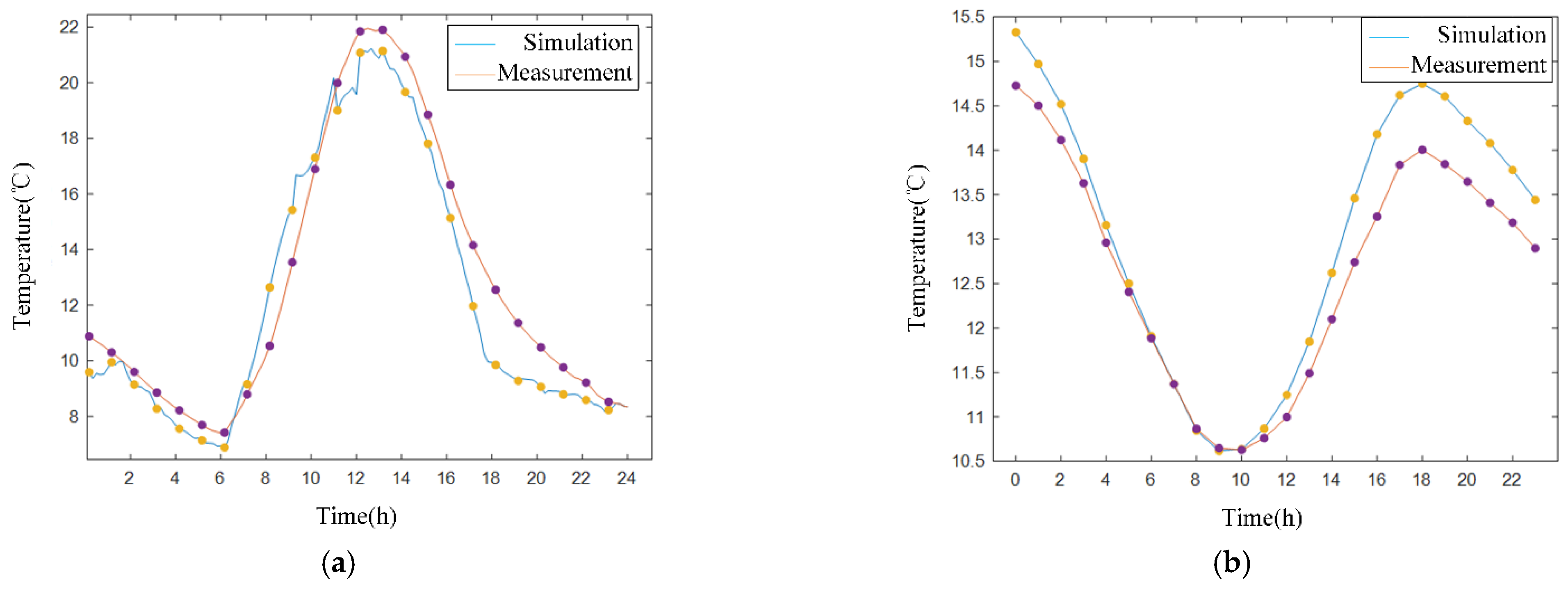
3.2.1. Comparison Results of Main Beam

In this section, the box girder (highway deck system) on the main girder of the cable-stayed bridge is selected as the object of study, the solid model of which is shown in Figure 13. The top deck directly bears the vehicle load and is an important part of the main truss box girder. The main structural material of the deck plate is steel. The material properties of the asphalt concrete layer of the deck differ greatly from those of the steel plate; the heat absorption coefficient of solar radiation is also different for the two materials. Both the steel plate and asphalt concrete are directly exposed to direct sunlight, and the temperature curves of the two fluctuate with different amplitudes during the day, with a maximum temperature difference of 20 °C between day and night. Therefore, they cannot be reduced to the same material in temperature field analysis. The mesh cell type of the asphalt concrete layer and the bridge deck is set in ANSYS using Solid90 cells with a known mesh size of 0.02 m. The FE model is illustrated in Figure 13 for 308,530 nodes and 117,955 cells.

This study applies a finite element analysis of ANSYS large-scale general-purpose calculation software (Ansys 2020 R2) to the structural health monitoring data of the Tongling Yangtze River Public-Rail Bridge based on the health-monitoring temperature and wind speed data as of 7 March 2019. Considering the effect of solar radiation, a temperature field simulation analysis is performed for the main span mid-section using thermal analysis type III boundary conditions, thereby establishing 144 load steps. Integrated temperature and heat transfer coefficients are applied to the boundary nodes of the steel box girders. The ANSYS post-processing POST1 function is used at the temperature clouds of the top plate of the upper box girder deck at each moment of the day to view the temperature clouds of each load step, as shown in Figure 14, with the time display ranging from 1:00 to 24:00 in two-hour intervals. The red area on the surface of the structure indicates the area with the highest temperature, whereas the blue area indicates the area with the lowest temperature. As observed in the figure, the highest temperature of the main beam appears at 14:00 every day, and the highest temperature appears on the surface of the main beam. In addition, the temperature inside the main beam does not change significantly.

The measurement points selected for the top surface are at the intersection of the asphalt pavement and steel plate, and the measurement points selected for the bottom plate are inside the bottom plate. As shown in Figure 15, the overall change curves of the calculated and actual monitoring values of the two measurement points are the same, and the monitoring values are very close to the simulated values; the error mainly stems from the inability to accurately obtain the wind speed on the surface of the structure. The difference between the two time series is small, which proves that the finite element simulation results are more accurate.

3.2.2. Comparison Results for Tower

This section studies the temperature field of the bridge tower structure using data collected on 7 March 2019. The temperature field analysis parameters are determined in the same way as in Section 3.2.1. The Tongling Bridge has two concrete bridge towers cast in C50 concrete in the north-south direction with a tower height of 220 m. Part of the bridge tower finite element model was established, with mesh refinement and applied load; the mesh size was set to 0.1 m, and the calculated sections and finite element model are shown in Figure 16. Solid90 was used in ANSYS to specify the necessary thermal analysis information not included in the data, such as the cell type and material thermophysical parameters. The setup of the measurement points is shown in Figure 11.

In the simulated temperature cloud of the bridge tower in Figure 17, it is proved that the effect of the dimensional change of the tower column along the vertical direction on the temperature is not considered in the case of no shading. The red area on the structural surface indicates the area with the highest temperature, whereas the blue area indicates the area with the lowest temperature. As shown in Figure 17, the highest temperature of the pylon is recorded at 14:00 every day. For solar radiation, the highest temperature appears on the surface of the tower, whereas the temperatures inside the tower hardly change. The simulated temperature data of the four facing central nodes (A1–A4) were extracted using the finite element model to represent the average temperature of the face. The simulated measurement point locations and temperature time curves are shown in Figure 18. In Figure 18 and Figure 19, it can be seen that the overall temperature change curves of the calculated and actual monitoring values of the two measurement points are the same. The monitoring values are close to the simulated values, and the errors satisfy the calculation accuracy requirements, which proves that the finite element simulation results are more accurate. Therefore, in the monitoring system, the boundary conditions are calculated, and the finite element simulation is performed using the fusion modeling method. The calculated results truly and effectively reflect the temperature field distribution of the bridge structure under the action of environmental conditions.

The temperature sensor was installed in the bridge tower, and the sensor was connected to the data collector. Subsequently, the data were transferred to the computer or monitoring system. This method allows the monitoring of temperature changes in real-time and for the historical data to be recorded for analysis and evaluation. In Figure 18 and Figure 19, it can be seen that the temperature curves of each surface are “sinusoidal”, with all surfaces exposed to direct solar radiation after sunrise. The peak of the temperature curves of A1 and A4 appear after 17:00, and the peak of the temperature curves of A2 and A3 appear around 14:00, which means that the two surfaces are exposed to direct solar radiation at different times; A1 and A4 mainly receive direct solar radiation in the afternoon, whereas A2 and A3 mainly receive direct solar radiation in the morning. The internal curve reflects the gentle temperature change inside the tower, which is attributed to the fact that the main material of the tower is concrete, which has poor thermal conductivity, and the tower is a closed-cavity structure not connected to the outside atmosphere. The average thickness of the tower is 3 m, making it difficult to transfer heat to the inner surface of the tower. A4 represents the northern side of the tower, which is subject to short direct solar radiation of low intensity, resulting in insignificant average temperature changes in this direction. Hence, the temperature difference between this face and the interior is minimal. Based on Figure 19b, the error between the finite element and measured results is consistently less than 1 °C, demonstrating the effectiveness and authenticity of the finite element simulation. During the initial stages of the simulation, iterative operations are necessary to stabilize the model over time. Consequently, the maximum error occurs at time 0, after which it remains consistently stable, maintaining an error below 1 °C.

3.3. Test

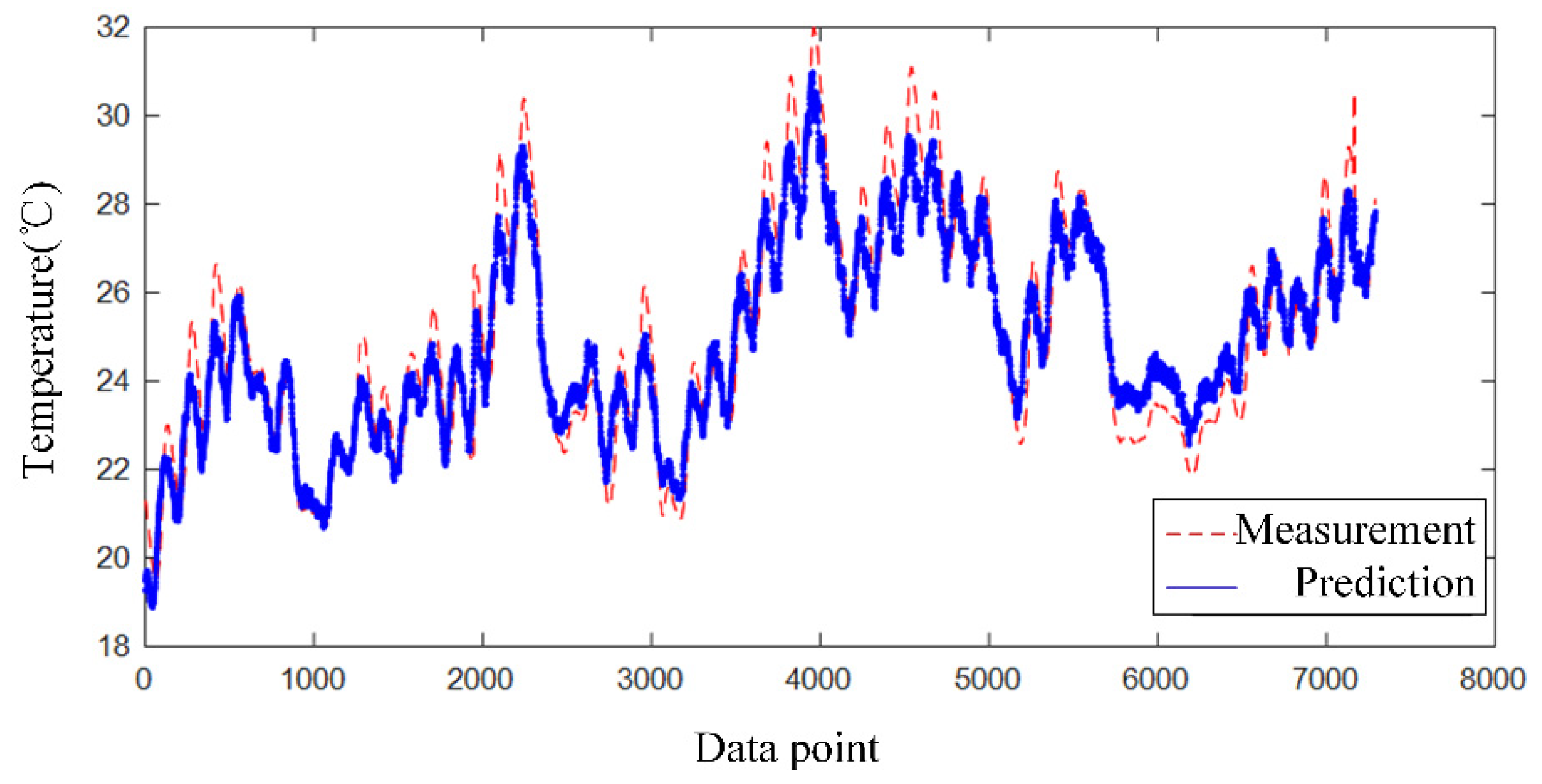
3.3.1. Temperature Mapping Model of Main Beam

In this section, the LSTM multi-source simulated temperature mapping model is used to effectively uncover the mapping relationships among the measurement points. First, the mapping model is established using the simulated data. Subsequently, the data are measured for the same points (01–03, 06–08) in the main span mid-section as input, and the measured data of 04–05 and 09–10 are also predicted using the simulated model, whereby the measured and simulated data are compared for 04–05 and 09–10. An error analysis is conducted to investigate whether the correlation information obtained by the simulated data correlation model is the same as that of the measured data.

To verify the stability of the simulated mapping model, the dataset in the main span of the SHM system of the Tongling Yangtze River bridge is calculated; the expanded dataset includes data from 5 December 2018 to 30 June 2019, covering a total of 207 days and 7 months, with a sampling frequency of 1 Hz. In addition, initially, 10-min averaged data are processed such that the number of data nodes after resampling is 29,808. The simulated and measured data after processing are shown in Figure 20.

The final prediction results of the multi-source mapping model for the long-term simulated data are shown in Figure 21, Figure 22, Figure 23 and Figure 24, taking measurement point 09 as an example.

Table 1. Performance results for long-term multi-source mapping model of the main beam.

Metric	Training Set	Test Set	Time
RMSE	0.4711	0.5791	39 s/25 s
Ta	0.0163	0.0243
R2	0.9935	0.9626

summarizes the computational results of the multi-source mapping model on the training and test sets.

The analysis in Table 1 shows that the two-layer LSTM neural network built based on long-term simulation data effectively explores the nonlinear relationship between different temperature measurement points and successfully predicts the change trend of data segments to extrapolate the fit of future data. As evaluation criteria, the RMSE metric is calculated, yielding approximately 1 for the slope k of the regression equation. The goodness of fit for both training and test sets are above 0.96; the RMSE and Ta are both small, indicating that the prediction effect of the simulation model satisfies the accuracy requirements, thus demonstrating the temporal stability and accuracy of the simulation mapping model.

The stability and accuracy of the simulation mapping model means that the established long-term simulation data mapping model is used here. The measured data at the same position of the main span mid-section (01–03 and 06–08) are input into the model for training, and the measured data at 04–05 and 09–10 are used as the evaluation criteria for the output data. The data predicted by the simulation model at the 04–05 and 09–10 measurement points are compared with the measured data at the 04–05 and 09–10 measurement points for error analysis. Taking measurement point 09 as an example, the final prediction effect of the multi-source mapping model for long-term simulation data is shown in the following

Table 2. Prediction effect of multi-source mapping model based on measured data in the main beam.

Metric	Measured Data	Time
RMSE	0.4879	18 s
Ta	0.0158
R2	0.9770

, Figure 25 and Figure 26:

From the graphical analysis in Figure 25 and Figure 26, it is observed that the slope of the regression equation is approximately 1. As evaluated by Table 2, the RMSE and Ta between the measured data and the data predicted by the simulation model are small, and Ta is less than 0.2, indicating that the model prediction results fulfill the actual engineering accuracy requirements. This proves that the predicted data generated by the multi-source simulation mapping model is similar to the actual sensor data, and the mapping relationship established by the correlation model is used to obtain long-term simulation data that match the actual data, effectively demonstrating the sameness of the spatial characteristic information between the simulated temperature and the actual temperature. Thus, the accuracy of the spatial expansion method based on digital fusion is demonstrated for the main beam temperature.

3.3.2. Temperature Mapping Model of Tower

The mapping model of the main girders was analyzed in the previous section, and this section uses the technique based on the LSTM network for the long-term simulation of the data to establish a mapping model for the bridge towers with LSTM network settings being the same as those of the multi-source mapping model of the main girders. The measured data of the same measurement points (three faces: south, east, and west) of the 3# bridge tower are accepted as input to predict the temperature data of the north face of the bridge tower using the simulation model. Comparisons and an error analysis are conducted for the north face temperature data predicted by the simulation model. The final prediction effect of the multi-source mapping model of the long-term simulation data is shown in

Table 3. Prediction effect of multi-source mapping model based on measured tower data.

Metric	Measured Data	Time
RMSE	1.1036	37 s
Ta	0.0491
R2	0.9824

. Figure 27 and Figure 28 show the correlation between the predicted data generated by the multi-source simulation mapping model and the measured data. The error between the measured and simulated data is low, demonstrating the robust and accurate performance of the proposed model.

In the graphical analysis presented in Figure 27 and Figure 28, the slope of the regression equation is approximately 1 according to RMSE and other evaluation criteria; the difference between measured and predicted data is small; and the Ta of the difference series is less than 0.2. This indicates that the bridge tower data predicted by the simulation model fulfill the accuracy requirements. The correlation model based on the long-term simulation data in each directional plane of the bridge tower also covers the correlation information between the measured data of the bridge tower. This demonstrates the significant correlation between the two types of data and the effectiveness of the spatial expansion method based on a numerical fusion of the bridge tower temperature data.

4. Conclusions

With a long-span cable-stayed bridge as the engineering background, in this study, the temperature collected by the health monitoring system is compared with complete simulated temperature field data obtained using a method based on integrated FE modeling. Based on the simulated and limited measurement data, a deep learning-based temperature spatial-expansion method is constructed, and the validity of the method is verified against the measured data of the main beam and bridge tower, thereby obtaining the optimal constructed value of the temperature of the stay cable and temperature field distribution of the entire bridge for a long period.

Combining the LSTM network structure and model optimization, the bridge temperature field information is effectively reconstructed, and missing information is filled. For the reconstruction of the temperature field of the main beam, the RMSE between the real and predicted values is 0.48, whereas the R2 between real and filled values is 0.97. For the reconstruction of the temperature field of the tower, the RMSE between the real and predicted values is 1.10, whereas the R2 between the real and filled values is 0.98. This provides a new and accurate solution for bridge safety state evaluation with full knowledge and control of the temperature load of the bridge. The method in this study has significance in terms of intelligent bridge monitoring.

References

1. Alvandi, A.; Cremona, C. Assessment of vibration-based damage identification techniques. J. Sound Vib. 2006, 292, 179–202. [Google Scholar] [CrossRef]
2. Bao, Y.; Chen, Z.; Wei, S.; Xu, Y.; Tang, Z.; Li, H. The State of the Art of Data Science and Engineering in Structural Health Monitoring. Engineering 2019, 5, 234–242. [Google Scholar] [CrossRef]
3. Xudong, J.; Huaqiang, Z.; Ye, X.; Limin, S. Faulty data detection and classification for bridge structural health monitoring via statistical and deep-learning approach. Struct. Control Health Monit. 2021, 28, e2824. [Google Scholar] [CrossRef]
4. Tang, F.; Ma, T.; Guan, Y.; Zhang, Z. Parametric modeling and structure verification of asphalt pavement based on BIM-ABAQUS. Autom. Constr. 2020, 111, 103066. [Google Scholar] [CrossRef]
5. Zhou, L.; Xia, Y.; Brownjohn, J.M.; Koo, K.Y. Temperature analysis of a long-span suspension bridge based on field monitoring and numerical simulation. J. Bridge Eng. 2016, 21, 04015027. [Google Scholar] [CrossRef]
6. Costin, A.; Hu, H.; Medlock, R. Building Information Modeling for Bridges and Structures: Outcomes and Lessons Learned from the Steel Bridge Industry. Transp. Res. Rec. 2021, 2675, 576–586. [Google Scholar] [CrossRef]
7. Tuceryan, M.; Chorzempa, T. Relative sensitivity of a family of closest-point graphs in computer vision applications. Pattern Recognition 1991, 24, 361–373. [Google Scholar] [CrossRef]
8. Omidshafiei, S.; Lopez, B.T.; How, J.P.; Vian, J. Hierarchical bayesian noise inference for robust real-time probabilistic object classification. arXiv 2016, arXiv:1605.01042. [Google Scholar]
9. Arazo, E.; Ortego, D.; Albert, P.; O’Connor, N.; McGuinness, K. Unsupervised label noise modeling and loss updating. In Proceedings of the International Conference on Machine Learning, Long Beach, CA, USA, 9–15 June 2019; ACM: New York, NY, USA, 2019; pp. 312–321. [Google Scholar]
10. Johnson, J.M.; Khoshgoftaar, T.M. A survey on classifying big data with label noise. ACM J. Data Inf. Qual. 2022, 14, 1–43. [Google Scholar] [CrossRef]
11. Lee, K.H.; He, X.; Zhang, L.; Yang, L. Cleannet: Transfer learning for scalable image classifier training with label noise. In Proceedings of the IEEE Conference on Computer Vision and Pattern Recognition, Lake City, UT, USA, 18–23 June 2018; pp. 5447–5456. [Google Scholar] [CrossRef] [Green Version]
12. Yeh, J.-R.; Shieh, J.-S.; Huang, N.E. Complementary Ensemble Empirical Mode Decomposition: A Novel Noise Enhanced Data Analysis Method. Adv. Adapt. Data Anal. 2011, 2, 135–156. [Google Scholar] [CrossRef]
13. Cao, J.; Liu, Y.; Li, C. Damage cross detection between bridges monitored within one cluster using the difference ratio of projected strain monitoring data. Struct. Health Monit. 2022, 21, 571–595. [Google Scholar] [CrossRef]
14. Zhang, S.; Liu, Y. Damage detection of bridges monitored within one cluster based on the residual between the cumulative distribution functions of strain monitoring data. Struct. Health Monit. 2020, 19, 1764–1789. [Google Scholar] [CrossRef]
15. Li, S.; Li, H.; Liu, Y.; Lan, C.; Zhou, W.; Ou, J. SMC structural health monitoring benchmark problem using monitored data from an actual cable-stayed bridge. Struct. Control Health Monit. 2014, 21, 156–172. [Google Scholar] [CrossRef]
16. He, Z.; Li, W.; Salehi, H.; Zhang, H.; Zhou, H.; Jiao, P. Integrated structural health monitoring in bridge engineering. Autom. Constr. 2022, 136, 104168. [Google Scholar] [CrossRef]
17. Bud, M.A.; Moldovan, I.; Radu, L.; Nedelcu, M.; Figueiredo, E. Reliability of probabilistic numerical data for training machine learning algorithms to detect damage in bridges. Struct. Control Health Monit. 2022, 29, e2950. [Google Scholar] [CrossRef]
18. Figueiredo, E.; Moldovan, I.; Santos, A.; Campos, P.; Costa, J.C.W.A. Finite element–based machine-learning approach to detect damage in bridges under operational and environmental variations. J. Bridge Eng. 2019, 24, 04019061. [Google Scholar] [CrossRef]
19. Sun, L.; Shang, Z.; Xia, Y.; Bhowmick, S.; Nagarajaiah, S. Review of bridge structural health monitoring aided by big data and artificial intelligence: From condition assessment to damage detection. J. Struct. Eng. 2020, 146, 04020073. [Google Scholar] [CrossRef]
20. Zhou, L.; Liang, C.; Chen, L.; Xia, Y. Numerical simulation method of thermal analysis for bridges without using field measurements. Procedia Eng. 2017, 210, 240–245. [Google Scholar] [CrossRef]
21. Huang, Y.; Liu, G.; Huang, S.; Rao, R.; Hu, C. Experimental and finite element investigations on the temperature field of a massive bridge pier caused by the hydration heat of concrete. Constr. Build. Mater. 2018, 192, 240–252. [Google Scholar] [CrossRef]
22. Mottershead, J.E.; Link, M.; Friswell, M.I. The sensitivity method in finite element model updating: A tutorial. Mech. Syst. Signal Process. 2011, 25, 2275–2296. [Google Scholar] [CrossRef]
23. Giagopoulos, D.; Arailopoulos, A.; Dertimanis, V.; Papadimitriou, C.; Chatzi, E.; Grompanopoulos, K. Structural health monitoring and fatigue damage estimation using vibration measurements and finite element model updating. Struct. Health Monit. 2019, 18, 1189–1206. [Google Scholar] [CrossRef]
24. Tang, X.; Wu, D.; Wang, S.; Pan, X. Research on Real-Time Prediction of Hydrogen Sulfide Leakage Diffusion Concentration of New Energy Based on Machine Learning. Sustainability 2023, 15, 7237. [Google Scholar] [CrossRef]
25. Nguyen-Da, T.; Li, Y.-M.; Peng, C.-L.; Cho, M.-Y.; Nguyen-Thanh, P. Tourism Demand Prediction after COVID-19 with Deep Learning Hybrid CNN–LSTM—Case Study of Vietnam and Provinces. Sustainability 2023, 15, 7179. [Google Scholar] [CrossRef]
26. Nabipour, M.; Nayyeri, P.; Jabani, H.; Mosavi, A.; Salwana, E.S.S. Deep Learning for Stock Market Prediction. Entropy 2020, 22, 840. [Google Scholar] [CrossRef]
27. Qu, C.X.; Yi, T.H.; Li, H.N.; Chen, B. Closely spaced modes identification through modified frequency domain decomposition. Measurement 2018, 128, 388–392. [Google Scholar] [CrossRef]
28. Qu, C.X.; Yi, T.H.; Li, H.N. Mode identification by eigensystem realization algorithm through virtual frequency response function. Struct. Control Health Monit. 2019, 26, e2429. [Google Scholar] [CrossRef]
29. Qu, C.X.; Liu, Y.F.; Yi, T.H.; Li, H.N. Structural Damping Ratio Identification through Iterative Frequency Domain Decomposition. J. Struct. Eng. 2023, 149, 04023042. [Google Scholar] [CrossRef]
30. Zhang, L. Analysis of energy saving effect of green building exterior wall structure based on ANSYS simulation analysis. Environ. Technol. Innov. 2021, 23, 101673. [Google Scholar] [CrossRef]
31. Zhu, Q.; Han, Q.; Liu, J.; Yu, C. High-Accuracy Finite Element Model Updating a Framed Structure Based on Response Surface Method and Partition Modification. Aerospace 2023, 10, 79. [Google Scholar] [CrossRef]
32. Yu, Y.; Si, X.; Hu, C.; Zhang, J. A review of recurrent neural networks: LSTM cells and network architectures. Neural Comput. 2019, 31, 1235–1270. [Google Scholar] [CrossRef] [PubMed]
Figure 1. Concrete material parameters: (a) heat transfer coefficient; (b) specific heat capacity.
Sustainability 15 09028 g001
Figure 2. Steel material parameters: (a) heat transfer coefficient; (b) specific heat capacity.
Sustainability 15 09028 g002
Figure 3. Flowchart of model updating.
Sustainability 15 09028 g003
Figure 4. Mapping generation flowchart.
Sustainability 15 09028 g004
Figure 5. BiLSTM neural network structure.
Sustainability 15 09028 g005
Figure 6. Schematic diagram of LSTM neural network.
Sustainability 15 09028 g006
Figure 7. Model establishment and optimization process.
Sustainability 15 09028 g007
Figure 8. Tongling Rail-cum-Road Changjiang River Bridge.
Sustainability 15 09028 g008
Figure 9. Layout of main beam sensors: (a) three-dimensional diagram; (b) pan view.
Sustainability 15 09028 g009
Figure 10. Temperature curve of the main beam.
Sustainability 15 09028 g010
Figure 11. Tower sensor distribution: (a) Association mode; (b) Sensor position.
Sustainability 15 09028 g011aSustainability 15 09028 g011b
Figure 12. Measured data from tower.
Sustainability 15 09028 g012
Figure 13. ANSYS model of Tongling Bridge box girder.
Sustainability 15 09028 g013
Figure 14. Temperature field of box girder at different times: (a) 1:00; (b) 6:00; (c) 10:00; (d) 14:00; (e) 18:00; (f) 22:00.
Sustainability 15 09028 g014aSustainability 15 09028 g014b
Figure 15. Comparison of simulated and measured temperatures: (a) box girder roof; (b) box girder bottom plate.
Sustainability 15 09028 g015
Figure 16. Element and finite element model of bridge tower (a) three-dimensional diagram; (b) element diagram.
Sustainability 15 09028 g016
Figure 17. Simulated temperature field of the tower at different times: (a) 1:00; (b) 6:00; (c) 10:00; (d) 14:00; (e) 18:00; (f) 22:00.
Sustainability 15 09028 g017aSustainability 15 09028 g017b
Figure 18. Finite element calculation results: (a) Simulated temperature of the bridge tower; (b) Sensor location.
Sustainability 15 09028 g018
Figure 19. Difference between measured data and simulations: (a) Measured temperature of the bridge tower; (b) Difference between measurements and finite element calculation results.
Sustainability 15 09028 g019
Figure 20. Main beam data after resampling: (a) Simulated data curves; (b) Measured data curves.
Sustainability 15 09028 g020
Figure 21. Performance of multi-source mapping model for measurement point 09 in measured data.
Sustainability 15 09028 g021
Figure 22. Correlational performance of multi-source mapping model for measurement point 09 in measured data.
Sustainability 15 09028 g022
Figure 23. Performance of multi-source mapping model for measurement point 09 in simulated data.
Sustainability 15 09028 g023
Figure 24. Correlational performance of multi-source mapping model for measurement point 09 in simulated data.
Sustainability 15 09028 g024
Figure 25. Performance of multi-source mapping model for curve fitting of deck data.
Sustainability 15 09028 g025
Figure 26. Performance of multi-source mapping model for deck data as scatter plot.
Sustainability 15 09028 g026
Figure 27. Performance of multi-source mapping model for tower data through a comparison of curves.
Sustainability 15 09028 g027
Figure 28. Scatter plot of the performance of multi-source mapping model for tower data.
Sustainability 15 09028 g028