Article

Vector Quantized Variational Autoencoder-Based Compressive Sampling Method for Time Series in Structural Health Monitoring

1
Elite Engineers School, Harbin Institute of Technology, 92 Xidazhi Street, Harbin 150001, China
2
Key Laboratory of Smart Prevention and Mitigation of Civil Engineering Disasters of the Ministry of Industry and Information Technology, School of Civil Engineering, Harbin Institute of Technology, 73 Huanghe Road, Harbin 150090, China
*
Author to whom correspondence should be addressed.
Sustainability 2023, 15(20), 14868; https://doi.org/10.3390/su152014868
Submission received: 22 August 2023 / Revised: 12 October 2023 / Accepted: 12 October 2023 / Published: 13 October 2023
(This article belongs to the Special Issue Artificial Intelligence (AI) in Structural Health Monitoring)

Abstract

:
The theory of compressive sampling (CS) has revolutionized data compression technology by capitalizing on the inherent sparsity of a signal to enable signal recovery from significantly far fewer samples than what is required by the Nyquist–Shannon sampling theorem. Recent advancement in deep generative models, which can represent high-dimension data in a low-dimension latent space efficiently when trained with big data, has been used to further reduce the sample size for image data compressive sampling. However, compressive sampling for 1D time series data has not significantly benefited from this technological progress. In this study, we investigate the application of different architectures of deep neural networks suitable for time series data compression and propose an efficient method to solve the compressive sampling problem on one-dimensional (1D) structural health monitoring (SHM) data, based on block CS and the vector quantized–variational autoencoder model with a naïve multitask paradigm (VQ-VAE-M). The proposed method utilizes VQ-VAE-M to learn the data characteristics of the signal, replaces the “hard constraint” of sparsity to realize the compressive sampling signal reconstruction and thereby does not need to select the appropriate sparse basis for the signal. A comparative analysis against various CS methods and other deep neural network models was performed in both synthetic data and real-world data from two real bridges in China. The results have demonstrated the superiority of the proposed method, with achieving the smallest reconstruction error of 0.038, 0.034 and 0.021, and the highest reconstruction accuracy of 0.882, 0.892 and 0.936 for compression ratios of 4.0, 2.66, and 2.0, respectively.

1. Introduction

With the increasing number of large-scale public infrastructure, structural health monitoring (SHM) technology has been more and more widely used in civil infrastructure in recent years, such as outlier diagnosis [1,2], damage identification [3,4], response prediction [5,6], and condition assessment [7,8], in order to reduce the risk of irreversible structural damage by continuous tracking of structural condition. However, a typical SHM system requires a large number of sensors to collect enough data for accurate inference of structural conditions. The need of collecting a massive amount of data leads to a tradeoff between the limited storage and data transmission capacity of the SHM system and the monitoring accuracy. Efficient data compression technology is the key to solve this difficult problem. In 2006, the compressive sampling (CS) method was proposed by Candes et al. [9] and Donoho [10], which has revolutionized the field of signal processing because of its ability to efficiently sense and compress signal simultaneously in bandwidth-constrained scenarios like SHM. If a signal can be represented by a sparse vector with a set of known basis functions, the CS method mathematically guarantees a high probability of reconstructing a signal compressed at a rate far less than the Nyquist sampling frequency. Its basic principle is to utilize the sparsity of a signal to constrain the ill-posed linear inverse problem. In addition, research about the robustness to uncertainty has always been a research priority in SHM due to environmental noise and insufficient data problems. For example, Zhao et al. [11] proposed a new paradigm of the recursive modeling strategy of Bayesian multiple linear regression for bridge deflection to deal with the interference from the data time lag and abnormal signal. Zhang et al. [12] presented a new modal parameter identification process based on the Gaussian mixture model of the data envelope and bandpass filtering. Motived by this, Bayesian probabilistic methods, which have been widely used in SHM data modeling [5,6,13] have also been extensively investigated in CS signal reconstruction, in which the confidence of the reconstructed signal can be quantified and the signal reconstruction robustness can be effectively enhanced [14,15].
In real-word applications, it is often difficult to find a sparse representation of many SHM signals. For example, while many time series signals are sparse after wavelet transform, this result does not apply to acceleration signals measured from some real structures [15], limiting the application of the CS method in many SHM applications. In recent years, many researchers have attempted to take advantage of the strong feature-learning ability of deep neural networks (DNNs) [16,17,18,19] to relieve the signal sparsity constraint in conventional CS, e.g., Bora et al. [20] proposed to use well-trained deep generative networks that capture the high-dimension image signals in a low-dimension space as an implicit regularizer for the ill-posed CS problem; Huang et al. [21] and Zhang et al. [22] successfully applied this idea to achieve high segmentation accuracy on building crack images with a high compression ratio; Dave et al. [23] proposed to use the architecture of an untrained deep convolutional generative adversarial networks as a prior to solve any differentiable linear inverse problem for image data, assuming such an architecture has already provided enough constraints to capture the underlying distribution of natural images [24].
Deep-learning-based CS methods have been successfully applied to many practical problems related to image or video signals [25,26,27,28], but 1D time series signals have not benefited from these advancements in CS. Ni et al. [29] directly used neural networks for compression and reconstruction of signals, which differs from the linear signal projection setup in the CS problem. There are studies on data loss recovery in SHM [30,31] using specially designed network structures that are not suitable for the general CS situation. To the best of our knowledge, however, there are seldom reports on significant improvement of CS for time series data based on deep learning. We speculate that the reason is the lack of efficient feature capturing neural network structures for time series. For example, the popular recurrent neural network (RNN) does not necessarily reduce the time series input to a very low-dimensional space. In fact, there is exponentially less volume for compression in 1D space than in higher dimensional spaces. Most of the successful time series models focus on modeling correlation structure at different length scales, such as the traditional autoregressive models.
In this paper, instead of following the standard approach to compress a signal in a single batch, we propose a new modeling approach based on block CS and VQ-VAE model with a multitask learning paradigm (VQ-VAE-M) for the 1D CS problem, which leverages the hierarchical structure of short-term and long-term correlations in time series. This method uses the VQ-VAE-M to learn the data characteristics of the signal, and replaces the “hard constraint” of sparsity to realize the compressive sampling signal reconstruction. Block CS has been studied by many researchers to speed up the reconstruction process [32,33,34,35]. Here, we investigate the potential of improving the reconstruction accuracy of the CS signal under high compression ratios by combining the idea of block CS and projection of short time series on a discrete space. The combination preserves the spatial position features between the elements in the signal effectively in the compression and reconstruction stages.
The remainder of this paper is organized as follows: Section 2 provides a concise explanation of conventional CS and block CS. The technical details of the proposed method are elaborated in Section 3. Then, we demonstrate the effectiveness of different DNNs applied to the 1D CS problem on both synthetic and real SHM data, including the basic multilayer perceptron (MLP) network, waveform transposed convolution neural network (WTCNN) (see Appendix A), waveform generative adversarial network (WaveGAN) (see Appendix B) [36], vector quantized–variational autoencoder (VQ-VAE) (see Appendix C) [37,38], and the proposed method in Section 4. Finally, we remark some concluding results and potential issues of our method in Section 5.

2. Compressive Sampling and Block Compressive Sampling

The conventional CS problem is basically solving the ill-posed inverse linear problem with l 1 regularization. Let us consider a linear transformation of N-dimensional discrete signal Χ = x 1 , x 2 , , x N T to W , which has only K (<<N) non-zero coefficients w i , based on a set of standard orthogonal basis vectors Ψ = ψ 1 , ψ 2 , , ψ N :
Χ = i = 1 N ψ i w i = Ψ W
Next, we compress the signal Χ to y by a random projection matrix: Φ t R M × N M N :
y = Φ t Χ = Φ t Ψ W = Θ W
where Θ = Φ t Ψ R M × N and y = y 1 , y 2 , , y N T R M × N . If Φ t satisfies the Restricted Isometry Property (RIP) condition, Candes et al. showed that we can reconstruct Χ from y with a high probability of success [9] by solving a non-linear optimization for X ^ :
X ^ = Ψ W ^   s . t .   W ^ = m i n W l 1
Φ t is typically taken as a Gaussian matrix with independent and identically distributed elements [9], but N can be very large for image signals, causing potential issues on the storage of the matrix and computation time of CS.
Gan et al. [39] studied a block CS method where the main idea is to divide X into Ρ short sequences x i of length b , and compress them into a sequence of short measurements y i of length a by the same projection matrix Φ b of size a × b . The reconstruction of X is achieved by concatenating the separately reconstructed X ^ i :
X ^ = Ψ b W ^   s . t .   W ^ = m i n W 1
Mathematically, it is equivalent to solving the original CS problem by designing Φ t as
Φ t = Φ b 0 0 Φ b L L 0 0 0 0 M M O M M 0 0 0 0 L L Φ b 0 0 Φ b
Recently, deep learning techniques have been applied on the block CS problem to improve computational accuracy and efficiency [40].
The hardware of the projection matrix in Equation (5) can be easily constructed by implementing a random 2D filter bank [39]. In the basic formulation of the block CS method, we assume that the small measurements are independent of each other. As a result, block artifacts usually appear at the boundaries of separations caused by non-smooth signal values as they are reconstructed separately. In our proposed method, we adopt the compression process of block CS to obtain smaller segments of time series signals. However, the reconstruction is not separated for each segment to avoid the block artifacts. Our main goal of using the block CS compression step is not to reduce storage size. As explained in the next section, the small signal segments match well with the neural network structure we picked to reconstruct the signals under a multitask framework.

3. Modified Block CS with VQ-VAE

The fundamental challenge of the CS problem is how to efficiently constrain the solution space of the ill-posed linear inverse problem based on the distribution of data. DNN can be seen as a tool to learn a representation of the underlying data distribution that can constrain the solution space through a set of data samples. This idea is typically implemented in two ways: (1) training a discriminative neural network that takes y as input and x as output; (2) training a generative neural network that transforms a low-dimensional distribution into the high-dimensional data distribution. In the former case, the trained DNN can be directly used as the signal decompressor, assuming that the learned patterns of decompressing signals from the data distribution are embedded in the trained network parameters. In the latter case, the low-dimensional space of the generative network input is optimized to decompress the signals, and the generative network is treated as an implicit constraint, replacing the sparsity constraint in the conventional CS [17].
In the next section, we demonstrate the unsatisfactory performance of these approaches on synthetic and real SHM data. We hypothesize that the state-of-the-art DNN architectures are not suitable for the 1D CS problem because it is difficult to find the compact representation of time series data in a low-dimension space. Therefore, instead of searching for a compact representation of the high dimension time series data directly, we try to take advantage of the hierarchical structure of short-term and long-term correlations in time series. Our proposed method is motivated by two main ideas: (1) using the block CS compression step to compress signal information within a short length scale, and (2) training a neural network that can assemble learned hidden features in the compressed signal segments to reconstruct the complete signal taking into account of the correlations across the short length scale segments. In particular, we implement the latter idea using a VQ-VAE model, which is originally designed as a generative model that projects a high dimension distribution into a discrete space. Different from the convention, our VQ-VAE model encodes the compressed data y into a discrete space and decodes them back into the original signal segment x directly.

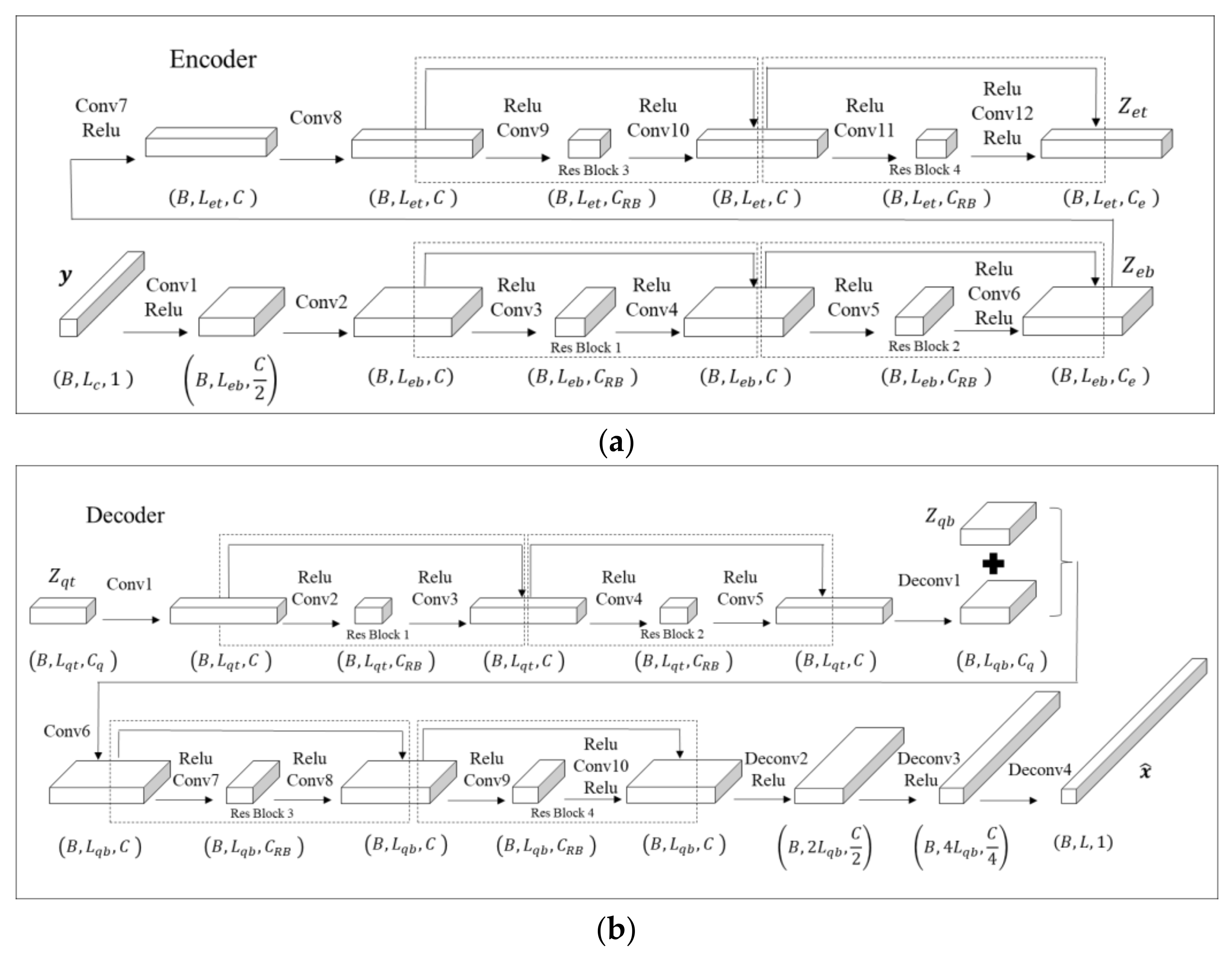
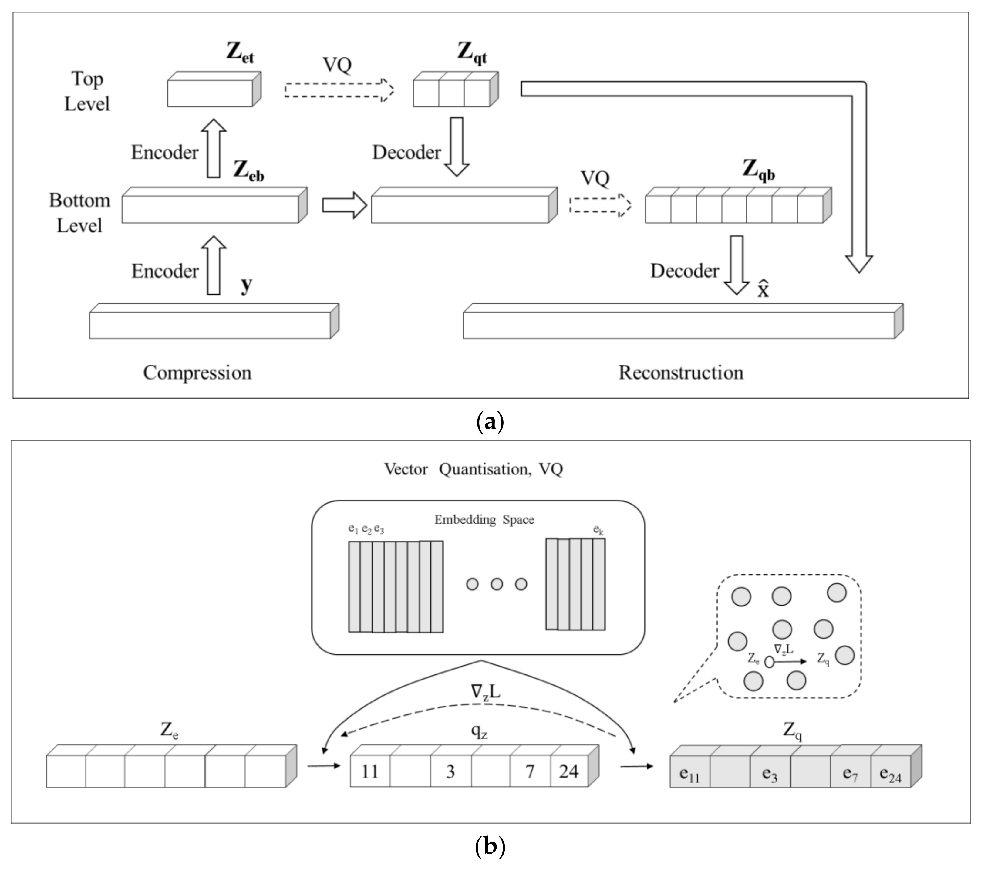
3.1. VQ-VAE Model with a Naïve Multitask Implementation

A vector quantized–variational autoencoder (VQ-VAE) [37,38] is basically a variational autoencoder (VAE) model with a discrete hidden space. The embedding space in a VQ-VAE model can be seen as a dictionary or codebook for the signals to be encoded. Once the model is trained, signals can be collected by drawing samples from the hidden space and passing them through the decoder part of the model. Here, we apply this model to decompress y back to x directly, i.e., a compressed signal y is fed into the encoder and decoder sequentially and the output is expected to be the decompressed signal x. This method is similar to the idea of designing over-complete dictionaries to solve the conventional CS problem [41,42,43,44], except that the codebooks in VQ-VAE are learned by training a DNN. However, applying VQ-VAE directly to CS does not lead to satisfactory results, as shown in the next section. Instead, we use block CS to compress a time series and input the concatenated vector y = y 1 , , y i , , y a of the compressed short data segments to VQ-VAE. This design is based on our speculation that it is easier to learn the decompression pattern if the short- and long-length scale correlations are separated. If we consider the decompression of each short segment y i as a single CS task, the concatenation of y i can be seen as using a naïve multitask learning approach to solve the block CS problem, allowing us to avoid the block artifact issue. At the same time, long-term correlation in the time series is less likely to be destructed during the compression step of block CS, i.e., implicitly separating the short-term and long-term correlation. We call our model VQ-VAE-M in this paper.
We adopt a 2-level VQ-VAE structure in this study according to the suggestions of Razavi et al. [38] (see Figure 1). First, the concatenated vector y is encoded into the top and bottom latent representations Z e t and Z e b by two encoders. Then, vector quantization is carried out according to the top codebook E t and bottom codebook E b , respectively, to obtain the top latent discrete representations Z q t and the bottom latent discrete representations Z q b (the quantization process of Z e b is guided by Z q t as well). Finally, Z q t and Z q b are passed to the decoder to reconstruct the original signal x. The vector quantization step simply replaces each value in Z e t and Z e b by the nearest neighbor value in the corresponding codebook E t and E b to form Z q t and Z q b . We employ convolutional layers in the encoder and decoder. Figure 2 shows the detailed structure and tensor sizes of the network, where B is the batch size of input, L c is the length of a single compressed signal in the input batch, L e b is the coding length of the bottom latent space, L e t is the coding length of the top latent space, C e is the number of latent coding channels, C R B is the number of residual block channels, L q t is the top latent discrete coding length, L q b is the bottom latent discrete coding length, C q is the number of latent discrete coding channels, and L is the original signal length. We note that our encoder and decoder are not symmetrical because the input and output are not in the same size. In order to extract deeper signal features and accelerate convergence, residual blocks and skip connections are used in both the encoder and the decoder.

3.2. DNN-Based CS Algorithm

In the proposed algorithm, we use the block CS compression step to linearly project a 1D signal x to y based on the matrix in Equation (5), and use VQ-VAE-M to reconstruct the original signal by feeding y into the input of VQ-VAE-M and taking the output as the reconstructed signal x directly. To train the VQ-VAE-M model, pairs of the original signal x and compressed signal y are collected to form a set of training data. In the case of SHM, time series data x from the sensors on a structure are collected and compressed into y. Following the typical neural network training scheme, the training dataset is separated into multiple batches, each of size B. During the backpropagation training phase, all batches of data are sequentially applied to a VQ-VAE-M model with randomly initialized parameters in a random order. The procedure of training with all batches is repeated N e p times (denoted as N e p epochs), until the parameter values converge. We adopt the same loss function as the original VQ-VAE model [38] in the backpropagation step:
L o s s x , D e = x D e 2 2 + s g E ( x ) e 2 2 + β s g e E x 2 2
where e denotes the quantized code of y, E denotes the encoder function, D denotes the decoder function, and s g refers to a stop-gradient operation.
In addition to the usual DNN hyperparameters, such as learning rate, batch size, and number of epochs, number of blocks in block CS (or the length of each data segment) is also an important hyperparameter in our algorithm, which controls the maximum length scale of information being compressed into y. The shorter the length of each data segment, the less expected amount of pattern we can observe from the data. As a result, it is easier for VQ-VAE-M to find a good representation in the discrete hidden space for the signal reconstruction task. However, the data compression space is also less, i.e., the minimum compression ratio is higher. As shown in the next section, our model favors shorter data segments for better reconstruction accuracy. Therefore, we choose the shortest possible segment length based on the desired compression ratio C R = N / M in most of our tests.

4. Results

In order to verify the reconstruction performance of the VQ-VAE-M method on CS signals, we test it on a set of synthetic times series constructed by superimposing sinusoidal signals and real acceleration time series obtained from SHM sensors on two real bridges in China (Tianjin Yonghe Bridge and Hangzhou Bay Bridge). Using the real bridge data, we compare our method with five conventional CS algorithms and four deep-learning-based CS algorithms to demonstrate the important contributions of block CS and DNN in the 1D CS problem. The five conventional CS algorithms based on sparse constraints are Basis Pursuit (BP) [9], Compressive sampling matching pursuit (CoSaMP) [45], Gradient Projection for Sparse Reconstruction (GPSR) [46], Bayesian compressive sensing (BCS) [47] and Bayesian compressive sensing integration over the prediction–error precision parameter (BCS-IPE) [14]. Among them, CoSaMP is a Greedy iterative algorithm, and BP and GPSR are two Convex optimization algorithms, all of which are well known and classic deterministic CS methods. BCS and BCS-IPE are two Bayesian probabilistic methods, which utilize sparse Bayesian learning to quantify the posterior uncertainty of the signal model and so can improve the signal reconstruction robustness. The four deep-learning-based CS algorithms are MLP, WTCNN, WaveGAN [36] and VQ-VAE [37,38]. The first two are discriminative-model-based methods, in which the MLP method is known to be simple and fast in calculation, and the WTCNN model has the advantages of fast training speed. WaveGAN and VQ-VAE are two most popular generative-model-based methods, as explained in the previous section. All four models are from our original design because of the lack of publicly available pretrained models for time series data using a deep-learning-based CS algorithm. The details of the structures and training procedures and advantages of these DNNs are shown in Appendix A, Appendix B and Appendix C. During the training procedure, early stopping [48] is employed to avoid overfitting and to select the network hyperparameters. In addition, data normalization and the two-tier network structure, which can improve the depth of the network structure and help to capture more characteristic information, are also employed to avoid underfitting.

4.1. Performance Metric

To evaluate the performance of signal reconstruction evaluation, the reconstruction error of a given signal is defined as follows:
E r = X ^ X 2 2 X 2 2
where X is the original signal and X ^ is the corresponding reconstructed signal. If the reconstruction error E r is less than or equal to a certain threshold δ , the reconstruction of the single signal is considered successful; otherwise, the reconstruction is considered failed. The ratio of the number of successfully reconstructed signals L s ( δ ) to the total number of signals L is used to quantify the reconstruction quality, which is called the reconstruction success rate:
S r = L s ( δ ) L
Various indicators are employed in the following tests and their results will be tabulated in Table 1, Table 2, Table 3, Table 4, Table 5, Table 6, Table 7, Table 8 and Table 9. Emean is the average reconstruction error of all test signals; E1 and E2 refer to the reconstruction success rate Sr for δ = 0.1 and δ = 0.2 , respectively; in addition, the average reconstruction time t of each signal and the training time ttrain for deep-learning-based methods are introduced; for cutting time series in the compression stage, the two cases of cutting sequence data into different blocks and no cutting are denoted as Multi-Blocks and Block, respectively. Among these indicators, we employ Emean to quantify the overall signal reconstruction accuracy at a certain compression ratio; E1 and E2 are used to measure how many signals can be reconstructed successfully. We also quantify the efficiency of the method by the indicators of average reconstruction time t and training time ttrain.
For conventional CS methods, the selection of sparse basis is often a necessary step. In this study, we try both cosine and wavelet bases for each method, and select the better result for comparison in order to demonstrate an advantage of the conventional methods.

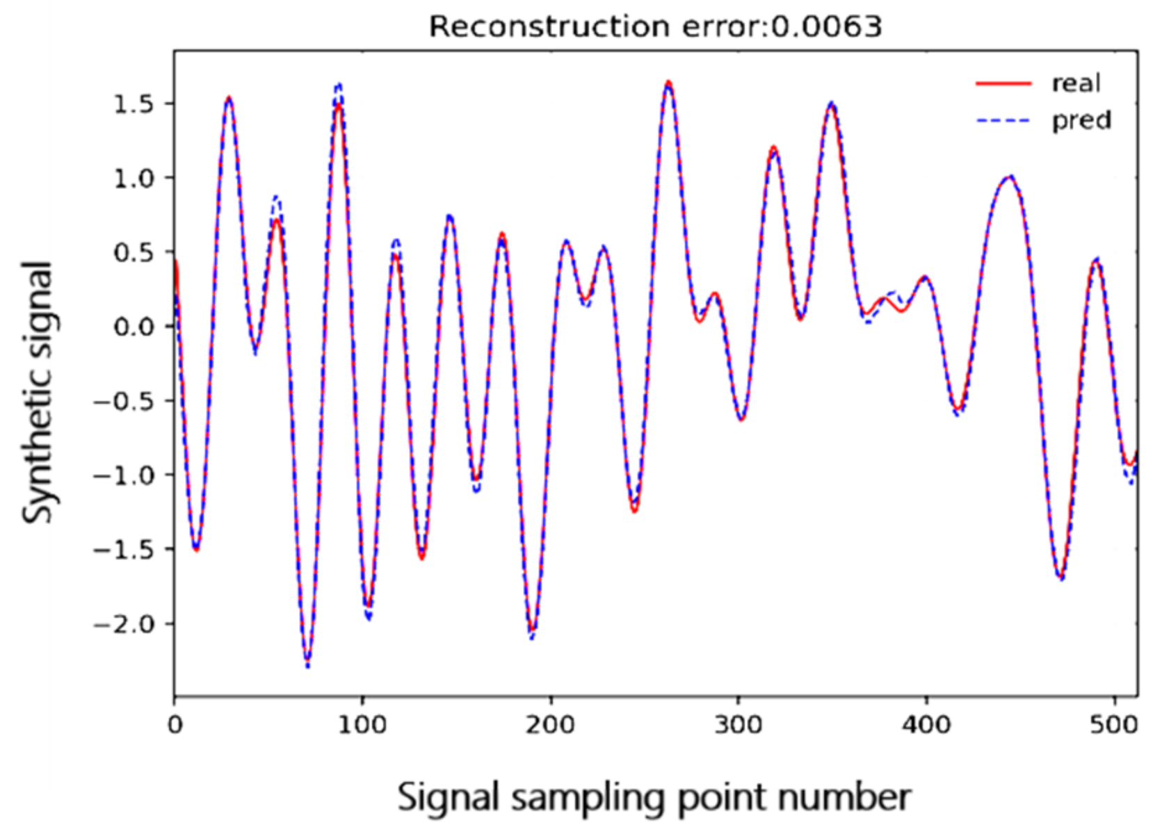
4.2. Test on Synthetic Data

We synthesized a total of 27,300 superimposed sinusoidal signals x of length 512 by
x = i = 1 10 A i sin ( w i t + φ i )
where A i , w i and φ i were sampled from U ( 0.1 ,   0.5 ) , U ( 1 ,   20 ) , U π ,   π ,   r e s p e c t i v e l y and U ( a , b ) denotes a uniform distribution between the interval of a and b. These signals were compressed to y by block CS with a compression ratio CR of N / M = 8 .0. We randomly selected 23,400 pairs of the x and y data to train the DNN models and tested them on the remaining signals along with various CS algorithms. Figure 3 shows a comparison of a synthetic signal and its reconstruction based on our proposed method. It can be seen that the two signals are consistent with each other very well, demonstrating the effectiveness of the method.
To investigate the robustness of the method, we repeated the experiment on each test signal 100 times and recorded the mean values of the performance metrics for three deep generative model-based methods VQ-VAE-M, WaveGAN and VQ-VAE. Table 1 lists the performance results of different CS methods. In terms of reconstruction quality, as expected, the reconstruction results of VQ-VAE-model-based algorithms are good because of their ability to learn from the data. The average reconstruction errors (Emean) of the two algorithms are significantly smaller compared with WaveGAN, where the error of VQ-VAE-M is only 0.003; in addition, the reconstruction success rates of both VQ-VAE-M and VQ-VAE methods are close to 1.
In terms of reconstruction speed, the VQ-VAE-M and VQ-VAE algorithms are fast on average. For the best performing model, VQ-VAE-M, it takes 0.038 s on average to reconstruct each signal and less than 3 min to train the model.

4.3. Test on Real SHM Data

In practical SHM applications, sensor signals often exhibit complex data characteristics, such as non-periodicity or contain various interference components due to environmental excitation, human disturbance, etc. Using two sets of real acceleration signals from Tianjin Yonghe Bridge and Hangzhou Bay Bridge, we inspected the performance of the proposed method and its sensitivity to the hyperparameters in block CS, noise contamination, and residual blocks and skip connections. Figure 4 shows the acceleration signals from the two bridges. We divided each time series into subsequences of length 512, yielding a total of 23,400 pieces of signals, and chose 23,010 pieces of signals as the training data set. Here, we judge whether the training data is sufficient based on the convergence of the loss function. In order to ensure that the model performs stably and reliably, the remaining signals were used as the validation data set. The validation data set should be selected randomly but cannot contain data from the training dataset [49]. Figure 5 shows a sample of signal from Tianjin Yonghe Bridge in different bases. We note that the signal is not very sparse in either cosine or wavelet basis, illustrating the difficulty of selecting a suitable basis for a conventional CS algorithm.

4.3.1. Sensitivity to Hyperparameters in Block CS

To understand the impact of the number of blocks N B and the length of each signal segment D B in block CS on the reconstruction performance, we compared the performance of VQ-VAE-M models with different D B and N B . The results in Table 2 and Table 3 show that a lower D B or higher N B is always preferred. This may indicate that finding a good representation of a long time series for solving the CS problem is difficult. Convolutional layers in DNNs (including VQ-VAE) are probably more effective for vectors with spatial correlation. Block CS with a high N B or low D B implies that most of the correlations in the time series are likely to be conserved. However, D B is the highest possible compression ratio in this case. Therefore, we suggest choosing the lowest possible D B corresponding to the desired compression ratio of a CS application in the applications.

4.3.2. Sensitivity to Noise Contamination

Noise contamination is a common issue in SHM signals. Sensitivity to noise is also related to the robustness of VQ-VAE-M and the possible overfitting problem. Here, we tested our method on the acceleration signal of Hangzhou Bay Bridge with a small signal-to-noise ratio. With a compression ratio of N / M = 4.0 , Figure 6 demonstrates the distribution of reconstruction errors as a function of δ . In general, the performance is not very satisfactory. Although the model cannot reconstruct complex signals completely, the low frequency components of complex signals can be reconstructed accurately. As shown in Figure 7, the reconstruction quality of signals in the time domain is poor and some peak values are not well reconstructed; however, in the frequency domain, the reconstruction quality of the low-frequency part is relatively good, while the reconstruction quality of the high-frequency part is relatively poor. This is because the neural network will pay more attention to the low-frequency components during the training phase, as has been previous suggested that the network fits low frequency before high frequency [50]. In fact, the natural frequency of bridge structure is generally low, as the high-frequency components are usually environmental noise. Therefore, even the proposed method cannot completely reconstruct the signal under particularly complex environmental excitation, it also has certain application potential in the field of SHM.

4.3.3. Sensitivity to Residual Blocks and Skip Connections

In order to extract signal features and accelerate convergence effectively, residual blocks and skip connections are used in both the encoder and decoder, as stated previously. We designed and performed ablation experiments on the acceleration signals from Tianjin Yonghe Bridge to demonstrate the effectiveness of these two modules. The compressive sampling signals were reconstructed at the compression ratios of 4.0, 2.66, 2.0, and the experiments were repeated 390 times for each compression ratio. The performance metric results of three methods were recorded in Table 4, Table 5 and Table 6, in which (VQ-VAE-M)E and (VQ-VAE-M)D show that residual blocks and skip connections are only used in the encoder or decoder, respectively.
From the results, it is concluded that the residual blocks and skip connections in both the encoder and decoder are conducive to reducing the reconstruction error and improving the reconstruction accuracy. Meanwhile, the residual blocks and skip connections in both the encoder and decoder can accelerate the model training convergence.

4.3.4. Comparison of Different CS Algorithms

As stated previously, we compared our proposed method with five conventional CS algorithms and four deep-learning-based CS algorithms on the acceleration signals of Tianjin Yonghe Bridge, which have a higher signal-to-noise ratio than those of Hangzhou Bay Bridge. At the compression ratios of 4.0, 2.66, 2.0, the compressive sampling signals were reconstructed by running the algorithms, and the experiments were repeated 390 times for each compression ratio. Table 7, Table 8 and Table 9 recorded the performance metrics of all 10 algorithms.
In terms of reconstruction quality, the deep-learning-based algorithms generally have better reconstruction results at the three compression ratios, showing that the compression patterns of the test data are successfully learnable from the training data. The Emean of MLP, WTCNN and VQ-VAE-M are all very small, where VQ-VAE-M has the smallest errors of 0.038, 0.034 and 0.021 at all three compression ratios, while the Emean of the traditional compressive sampling algorithms are larger than 0.2, which are relatively high. In terms of E1 and E2, the indices values of deep-learning-based algorithms are also much higher than traditional methods. Among them, VQ-VAE-M algorithm has the highest E1 accuracy of more than 0.88 when the compression ratio N / M is 4.0, while the highest E1 accuracy of traditional algorithm is 0.10. The situation is similar in E2, where the VQ-VAE-M algorithm obtains the highest E2 accuracy of more than 0.98. Similar conclusion can be observed in Table 7, Table 8 and Table 9 when the compression ratios N / M are 2.66 and 2.0, respectively.
In terms of signal reconstruction speed, the three deep-learning-based algorithms MLP, WTCNN and VQ-VAE-M are much faster on average. For the best performing model, VQ-VAE-M, it takes only 0.013 s on average to reconstruct each signal, which is much faster than WaveGAN and VQ-VAE, and most traditional methods.
In the application, if E1 or E2 equals to 1.0, we consider the signal reconstruction is successful. The results in Table 7, Table 8 and Table 9 show that the maximum compression ratio of our method is around 2.0 for the acceleration signals from Tianjin Yonghe Bridge. It is also observed that the traditional compressive sampling methods and other deep-learning-based compressive sampling methods fail to reconstruct all signals successfully at this compression ratio. Therefore, our method achieves the highest compression ratio compared to other methods.
It is concluded that compared with the traditional compressive sampling methods based on sparse constraint, the compressive sampling signal reconstruction method based on VQ-VAE-M significantly improves the reconstruction quality and the reconstruction speed, while being able to achieve a high-quality reconstruction of one-dimensional SHM compressive sampling signal at a high compression ratio (Figure 8).

5. Conclusions

The traditional compressive sampling methods require the signal to satisfy the “hard constraint” of sparsity in a certain transform domain. However, the civil structural response is not only related to the sparsity of modes, but also affected by the structural excitation. The sparsity is sometimes difficult to be satisfied in the case of complex environmental interference. In this paper, based on block CS and the vector quantized–variational autoencoder model with a naïve multitask paradigm (VQ-VAE-M), a data driven-based compressive sampling signal reconstruction method for one-dimensional time series signals in SHM is studied. The main contents can be summarized as follows:
(1)
Based on the vector quantized–variational autoencoder model with a naïve multitask paradigm (VQ-VAE-M), a one-dimensional compressive sampling signal reconstruction method is established. This method uses VQ-VAE-M to learn the data characteristics of the signal, replaces the “hard constraint” of sparsity to realize the compressive sampling signal reconstruction and so eliminate the need to select the appropriate sparse basis for the signal. VQ-VAE-M embeds and maintains one or more codebooks in the latent space to reconstruct signal. The unique bottleneck structure improves the depth of the network, and the two-tier network structure enriches the details of the reconstructed signal. In addition, the model combined with the block random Gaussian projection matrix can preserve the spatial position features between the elements in the signal as much as possible in both the compression and reconstruction stages, which greatly reduces the difficulty of decoupling in decompression and reconstruction, and ensures the quality and speed of signal reconstruction.
(2)
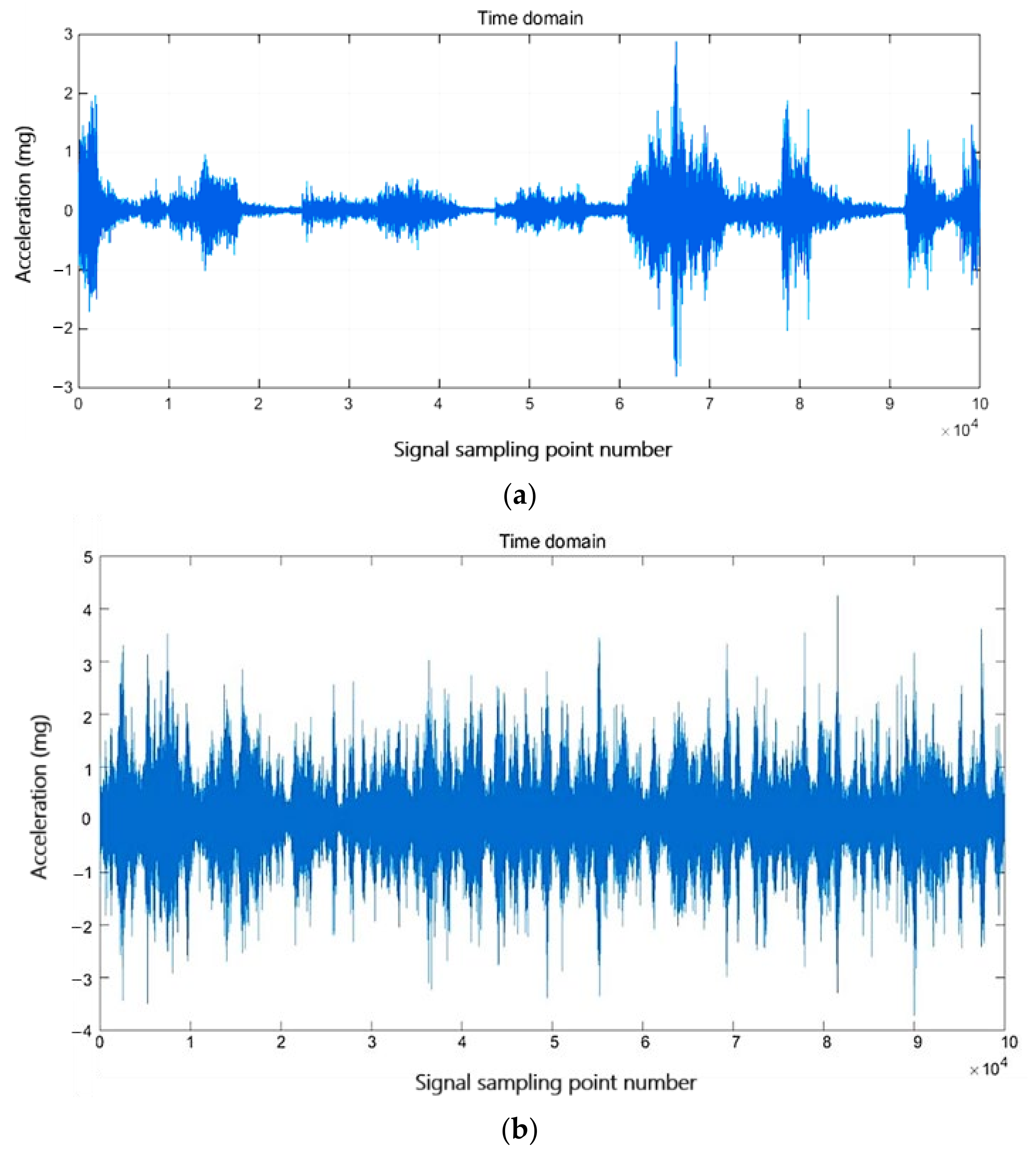
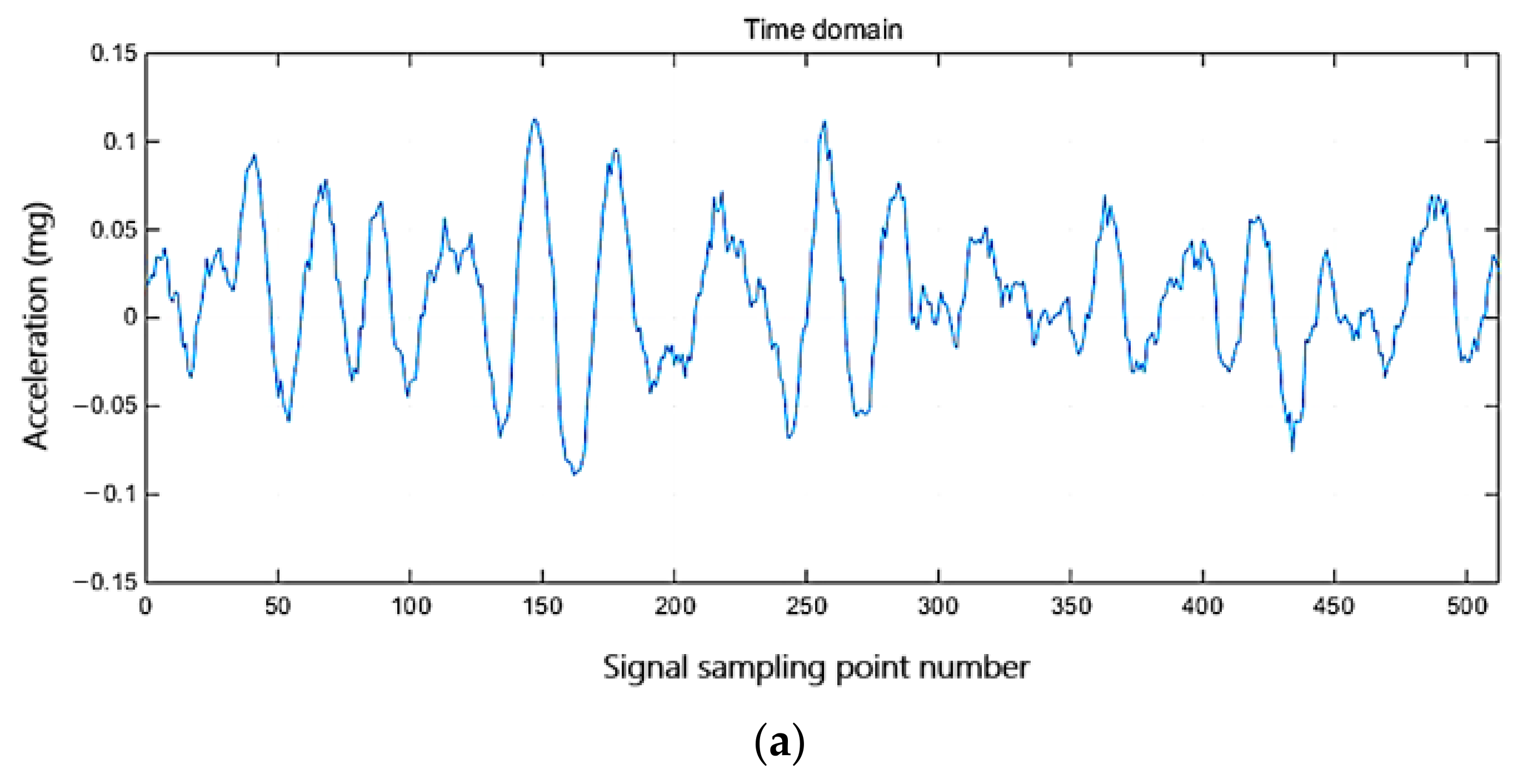
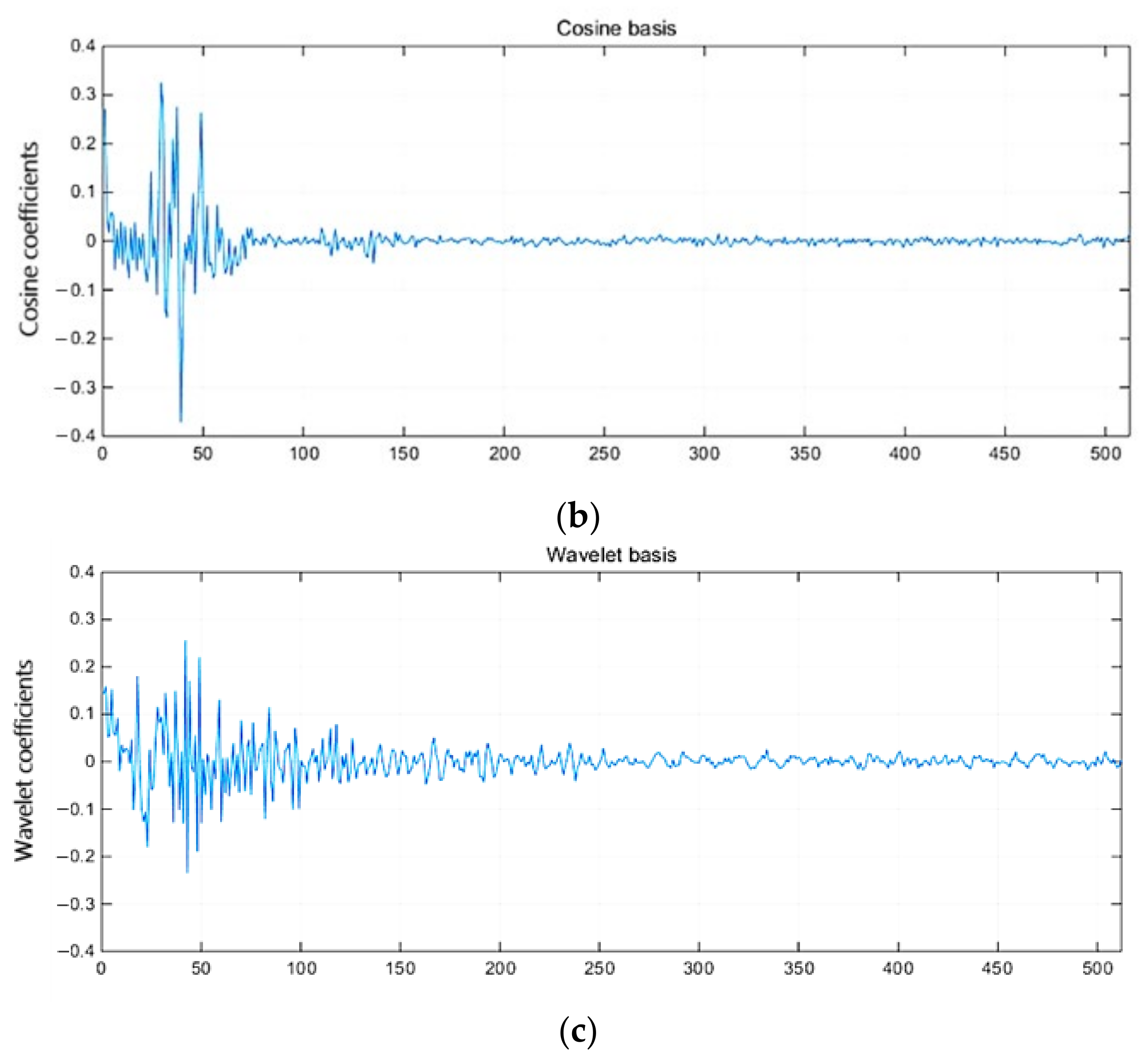
The superimposed sinusoidal synthetic signal (sparse enough in the frequency domain) and Yonghe Bridge acceleration signal (not sparse enough on both the cosine basis and wavelet basis) are used to verify the performance of the proposed method, which is compared with the other compressive sampling methods. The results show that the proposed method obviously has better performance, that is, higher reconstruction quality, faster reconstruction speed, enabling to reconstruct signal at a higher compression ratio, and no need to select the appropriate sparse basis for the signal.
(3)
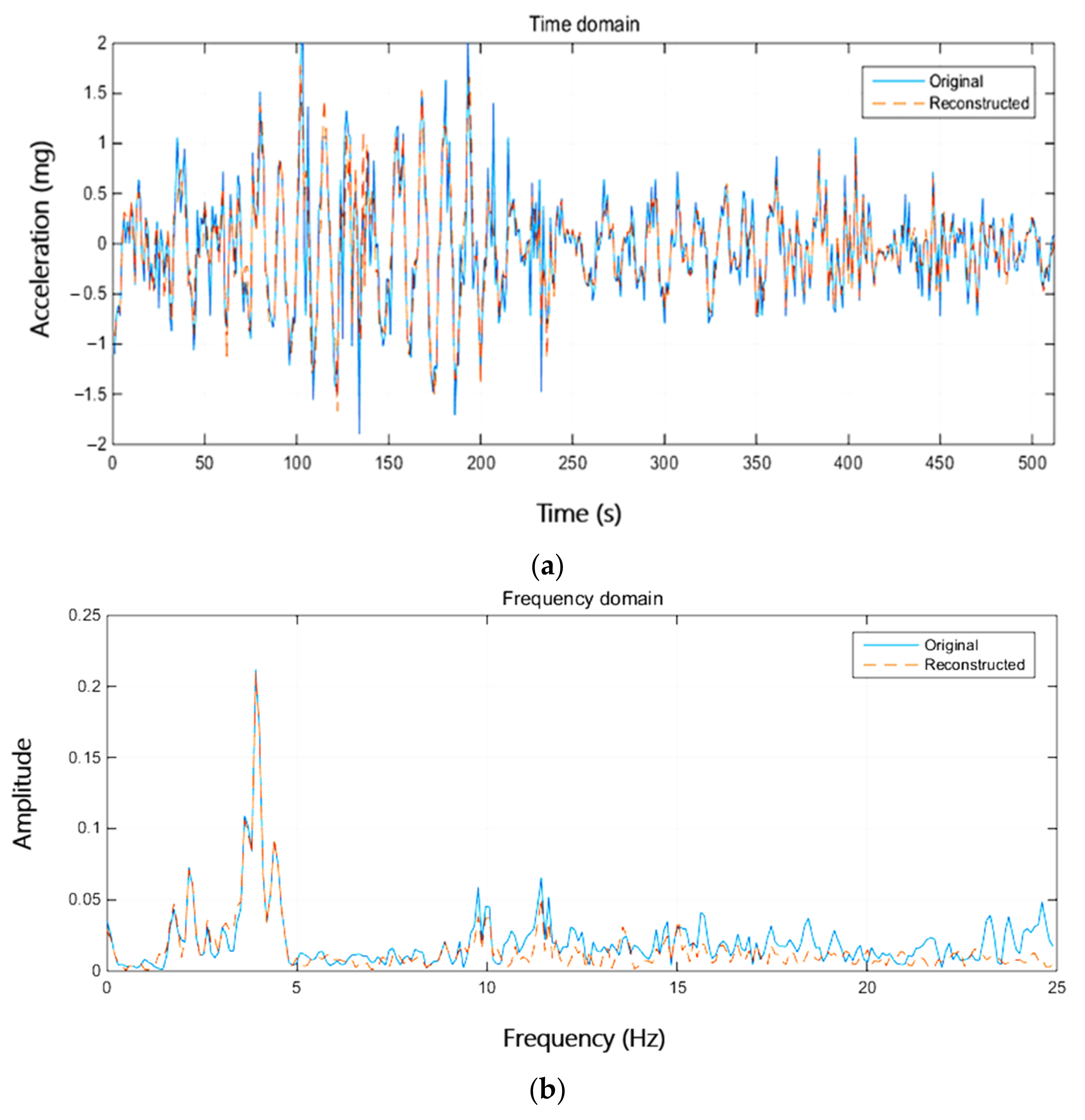
The characteristics and advantages of the block random Gaussian projection matrix are analyzed. The matrix can preserve the spatial features between the elements in the signal, which is not only conducive to decoupling, but also to extracting the overall characteristics of adjacent signals. In addition, the reconstruction performance of this method in complex environment is also investigated. Even if the environment excitation is more complex, the method can still reconstruct the information of the low-frequency components of the signal effectively.
This method also has some limitations: a large number of data are required to train the neural network model aiming at different compressive sampling signal types, and the reconstruction performance of complex and high-dimensional signals can be further improved. In future study, it will be useful to combine the proposed method with a Transfomer model and Bayesian probabilistic method to address these issues.

Author Contributions

Conceptualization, G.L., Z.J. and Y.H.; methodology, G.L., Z.J. and K.H.; software, G.L., Q.Z. and K.H.; validation, G.L. and Y.H.; formal analysis, G.L., Q.Z. and Y.H.; investigation, Z.J. and K.H.; data curation, K.H. and Q.Z.; writing—original draft preparation, G.L., Z.J. and K.H.; writing—review and editing, Z.J. and Y.H. All authors have read and agreed to the published version of the manuscript.

Funding

The study was supported by National Natural Science Foundation of China under Grant Nos. U2139209 and 52078174.

Data Availability Statement

Not applicable.

Conflicts of Interest

The authors declare no conflict of interest.

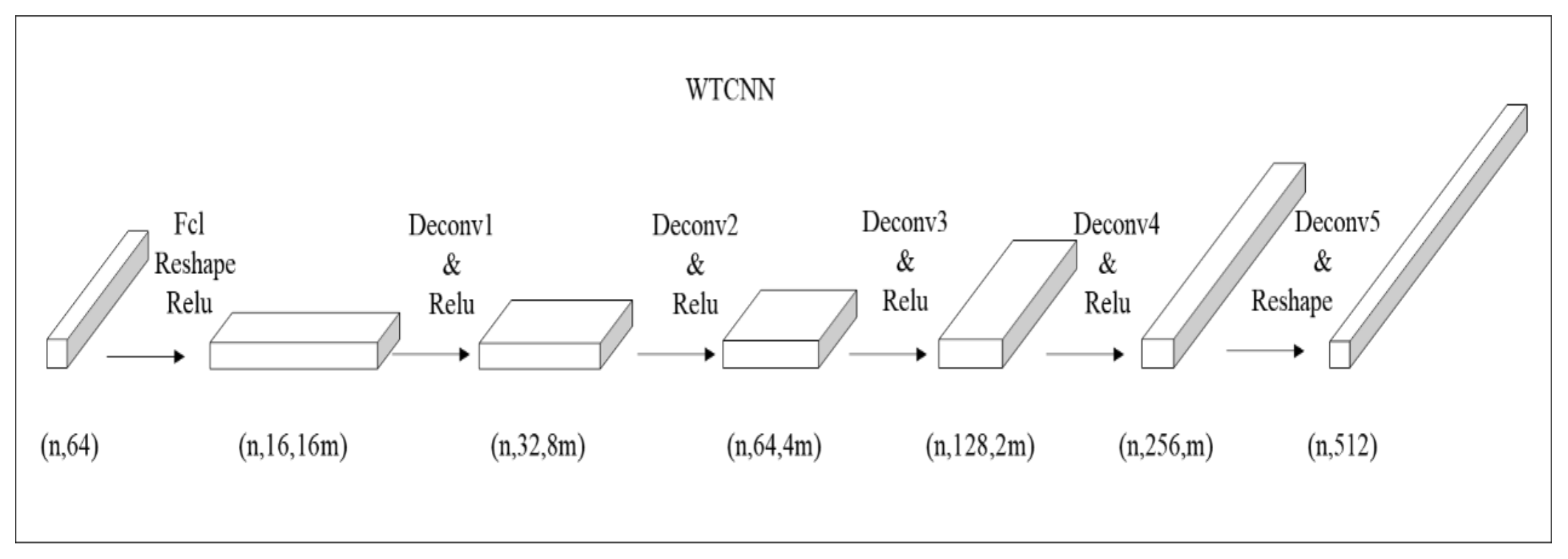
Appendix A. Waveform Transposed Convolution Neural Networks
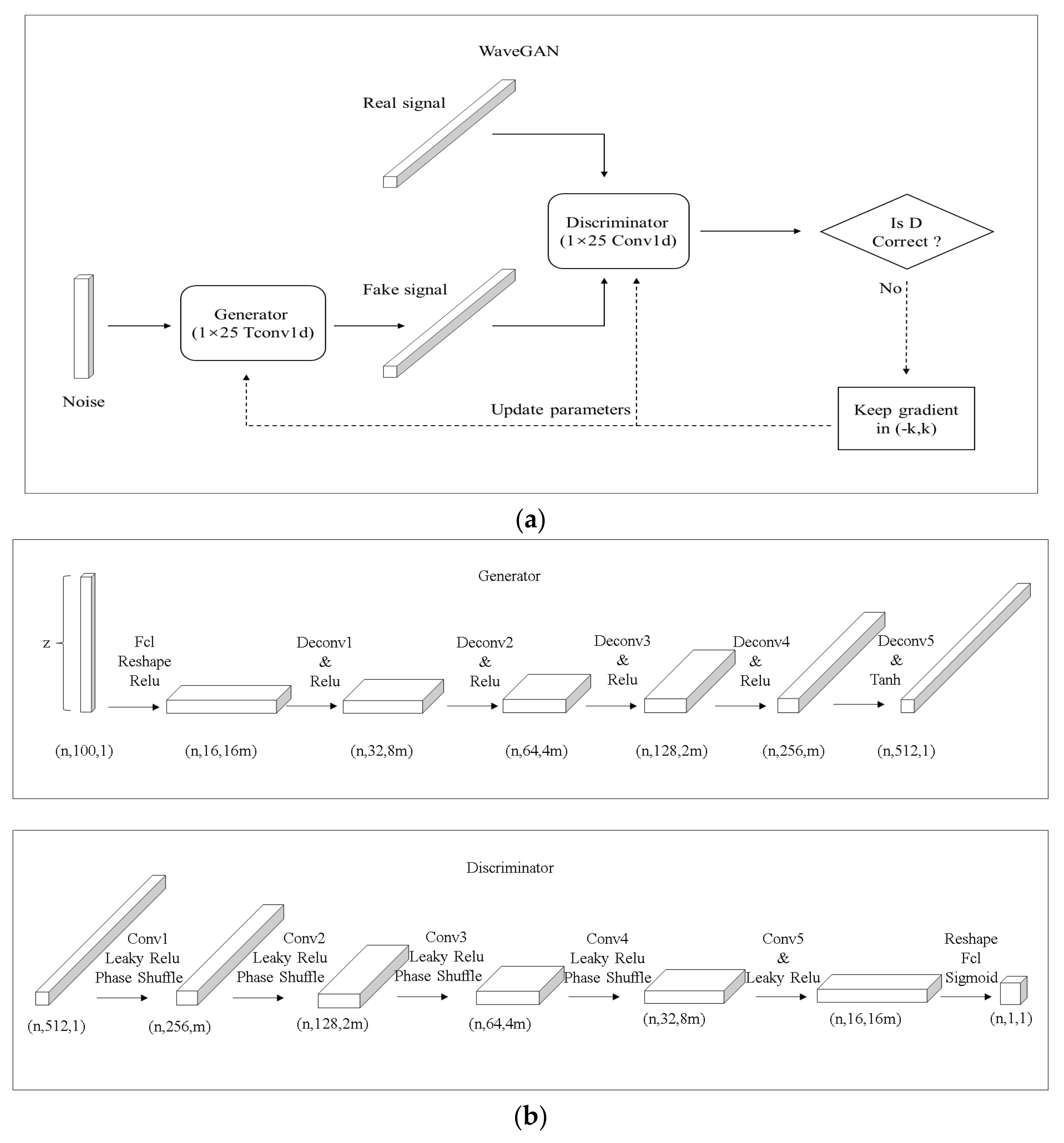
The idea of Waveform Transposed Convolution Neural Networks (WTCNN) is derived from WaveGAN, which mainly consists of one-dimensional transposed convolution layers with larger receptive field, and has the advantages of less parameters and fast training.
When reconstructing the signal based on the WTCNN, the constructed network is shown in Figure A1. In order to increase the receptive field, the size of the transposed convolution kernel is taken as 25 and the step size is taken as 2. The selected loss function is shown in Equation (A1):
E = 1 2 L X ^ X 2 2
Figure A1. Structure diagram of WTCNN.
Sustainability 15 14868 g0a1

Appendix B. WaveGAN

WaveGAN is a generative adversarial model specially designed for a one-dimensional signal, which mainly includes the following features: using one-dimensional convolution instead of two-dimensional convolution to process one-dimensional signal; using larger convolution kernel and step size to increase receptive field; and using a WGAN-GP training mechanism to improve training stability and reduce the disadvantage of generative adversarial model that it is difficult to converge. WaveGAN can also be used to reconstruct compressive sampling signal, which consists of two steps: (1) constructing generative network with the ability of generating quasi-realistic signals; and (2) selecting the most possible reconstructed signal by optimizing the compressed projection.
Here, signal reconstruction is carried out based on WaveGAN, and the constructed network is shown in Figure A2. The network consists of generator G and discriminator D arranged symmetrically. The selected loss function is shown in Equation (A2):
E z = E x ~ ~ P g D x ~ E x ~ P r D x + λ E x ^ ~ P x ^ x ^ D ( x ^ ) 2 1 2
The selected optimization function is shown in Equation (A3):
E ( z ) = Φ G ( z ) y 2 2
where Φ is the projection matrix, y is the compressed projection and z is the hidden variable. By minimizing the objective function, we can find the optimal hidden variable z ^ corresponding to x , and then input it into G to reconstruct the signal x ^ = G ( z ^ ) .
Figure A2. (a) Structure diagram of WaveGAN. (b) Generator and discriminator of WaveGAN.
Sustainability 15 14868 g0a2

Appendix C. Vector Quantized–Variational AutoEncoder

VQ-VAE has been introduced in the previous paper, and the network structure and loss function are basically the same. The VQ-VAE model has the advantage of generating results comparable to the current state-of-the-art generative models without encountering the posteriori collapse problem. The reconstruction of compressive sampling signal can also be realized by using VQ-VAE, and the selected optimization function is shown in Equation (A4):
E x ^ t = Φ D e E n ( x ^ t ) y t 2 2 + β Z e x ^ t s g e 2 2
where x ^ t is the reconstructed signal, y t is the compressed projection and β is the weight hyperparameter. By minimizing the objective function, the optimal reconstructed signal x ^ t can be found.

References

  1. Li, Q.; Gao, J.; Beck, J.L.; Lin, C.; Li, H. Probabilistic outlier detection for robust regression modeling of structural response for high-speed railway track monitoring. Struct. Health Monit. 2023, 14759217231184584. [Google Scholar] [CrossRef]
  2. Song, J.; Zhang, S.; Tong, F.; Tong, F.; Yang, J.; Zeng, Z.; Yuan, S. Outlier Detection Based on Multivariable Panel Data and K-Means Clustering for Dam Deformation Monitoring Data. Adv. Civ. Eng. 2021, 2021, 3739551. [Google Scholar] [CrossRef]
  3. Liu, T.; Xu, H.; Ragulskis, M.; Cao, M.; Ostachowicz, W. A data-driven damage identification framework based on transmissibility function datasets and one-dimensional convolutional neural networks: Verification on a structural health monitoring benchmark structure. Sensors 2020, 20, 1059. [Google Scholar] [CrossRef] [PubMed]
  4. Wang, Q.A.; Dai, Y.; Ma, Z.G.; Ni, Y.Q.; Tang, J.Q.; Xu, X.Q.; Wu, Z.Y. Towards probabilistic data-driven damage detection in SHM using sparse Bayesian learning scheme. Struct. Control Health Monit. 2022, 29, e3070. [Google Scholar] [CrossRef]
  5. Wang, Q.A.; Wang, C.B.; Ma, Z.G.; Chen, W.; Ni, Y.Q.; Wang, C.F.; Yan, B.G.; Guan, P.X. Bayesian dynamic linear model framework for structural health monitoring data forecasting and missing data imputation during typhoon events. Struct. Health Monit. 2022, 21, 2933–2950. [Google Scholar] [CrossRef]
  6. Wang, Q.A.; Dai, Y.; Ma, Z.G.; Wang, J.F.; Lin, J.F.; Ni, Y.Q.; Ren, W.X.; Jiang, J.; Yang, X.; Yan, J.R. Towards high-precision data modeling of SHM measurements using an improved sparse Bayesian learning scheme with strong generalization ability. Struct. Health Monit. 2023, 14759217231170316. [Google Scholar] [CrossRef]
  7. Wei, S.; Zhang, Z.; Li, S.; Li, H. Strain features and condition assessment of orthotropic steel deck cable-supported bridges subjected to vehicle loads by using dense FBG strain sensors. Smart Mater. Struct. 2017, 26, 104007. [Google Scholar] [CrossRef]
  8. Sony, S.; Dunphy, K.; Sadhu, A.; Capretz, M. A systematic review of convolutional neural network-based structural condition assessment techniques. Eng. Struct. 2021, 226, 111347. [Google Scholar] [CrossRef]
  9. Candes, E.J.; Romberg, J.; Tao, T. Robust uncertainty principles: Exact signal reconstruction from highly incomplete frequency information. IEEE Trans. Inf. Theory 2006, 52, 489–509. [Google Scholar] [CrossRef]
  10. Donoho, D.L. Compressed sensing. IEEE Trans. Inf. Theory 2006, 52, 1289–1306. [Google Scholar] [CrossRef]
  11. Zhang, H.; Ding, Y.; Meng, L.; Qin, Z.; Yang, F.; Li, A. Bayesian Multiple Linear Regression and New Modeling Paradigm for Structural Deflection Robust to Data Time Lag and Abnormal Signal. IEEE Sens. J. 2023, 23, 19635–19647. [Google Scholar]
  12. Zhang, H.; Ding, Y.; Li, A.; Qin, Z.; Chen, B.; Zhang, X. State-monitoring for abnormal vibration of bridge cables focusing on non-stationary responses: From knowledge in phenomena to digital indicators. Measurement 2022, 205, 112418. [Google Scholar]
  13. Wang, Q.A.; Zhang, C.; Ma, Z.G.; Ni, Y.Q. Modelling and forecasting of SHM strain measurement for a large-scale suspension bridge during typhoon events using variational heteroscedasic Gaussian process. Eng. Struct. 2021, 251, 113554. [Google Scholar] [CrossRef]
  14. Huang, Y.; Beck, J.L.; Wu, S.; Li, H. Bayesian compressive sensing for approximately sparse signals and application to structural health monitoring signals for data loss recovery. Probabilistic Eng. Mech. 2016, 46, 62–79. [Google Scholar] [CrossRef]
  15. Huang, Y.; Beck, J.L.; Wu, S.; Li, H. Robust Bayesian compressive sensing for signals in structural health monitoring. Comput. -Aided Civ. Infrastruct. Eng. 2014, 29, 160–179. [Google Scholar] [CrossRef]
  16. Jogin, M.; Madhulika, M.S.; Divya, G.D.; Meghana, R.K.; Apoorva, S. Feature Extraction using Convolution Neural Networks (CNN) and Deep Learning. In Proceedings of the 3rd IEEE International Conference on Recent Trends in Electronics, Information & Communication Technology (RTEICT), Bangalore, India, 18–19 May 2018. [Google Scholar]
  17. Shaheen, F.; Verma, B.; Asafuddoula, M. Impact of Automatic Feature Extraction in Deep Learning Architecture. In Proceedings of the 2016 International Conference on Digital Image Computing: Techniques and Applications (DICTA), Gold Coast, QLD, Australia, 1–3 December 2017. [Google Scholar]
  18. Hatir, M.E.; Ince, I. Lithology mapping of stone heritage via state-of-the-art computer vision. J. Build. Eng. 2021, 34, 101921. [Google Scholar] [CrossRef]
  19. Hatır, E.; Korkanç, M.; Schachner, A.; Ince, I. The deep learning method applied to the detection and mapping of stone deterioration in open-air sanctuaries of the Hittite period in Anatolia. J. Cult. Herit. 2021, 51, 37–49. [Google Scholar] [CrossRef]
  20. Bora, A.; Jalal, A.; Price, E.; Dimakis, A.G. Compressed sensing using generative models. In Proceedings of the International Conference on Machine Learning (PMLR), Amsterdam, The Netherlands, 7–10 July 2017. [Google Scholar]
  21. Huang, Y.; Zhang, H.Y.; Li, H.; Wu, S. Recovering compressed images for automatic crack segmentation using generative models. Mech. Syst. Signal Process. 2021, 146, 107061. [Google Scholar] [CrossRef]
  22. Zhang, H.Y.; Wu, S.; Huang, Y.; Li, H. Robust multitmask compressive sampling via deep generative models for crack detection in structural health monitoring. Struct. Health Monit. 2023, 14759217231183663. [Google Scholar] [CrossRef]
  23. Dave, V.V.; Jalal, A.; Soltanolkotabi, M.; Price, E.; Vishwanath, S.; Dimakis, A.G. Compressed Sensing with Deep Image Prior and Learned Regularization. arXiv 2018, arXiv:1806.06438. [Google Scholar]
  24. Ulyanov, D.; Vedaldi, A.; Lempitsky, V. Deep Image Prior. In Proceedings of the IEEE Conference on Computer Vision and Pattern Recognition (CVPR), Salt Lake City, UT, USA, 18–23 June 2018. [Google Scholar]
  25. Iliadis, M.; Spinoulas, L.; Katsaggelos, A.K. Deep fully-connected networks for video compressive sensing. Digit. Signal Process. 2018, 72, 9–18. [Google Scholar] [CrossRef]
  26. Chen, B.; Zhang, J. Content-Aware Scalable Deep Compressed Sensing. IEEE Trans. Image Process. 2022, 31, 5412–5426. [Google Scholar] [CrossRef]
  27. Wang, Z.F.; Wang, Z.H.; Zeng, C.Z.; Yu, Y.; Wan, X.K. High-Quality Image Compressed Sensing and Reconstruction with Multi-scale Dilated Convolutional Neural Network. Circuits Syst. Signal Process. 2023, 42, 1593–1616. [Google Scholar] [CrossRef]
  28. Yang, G.; Yu, S.; Dong, H.; Slabaugh, G.; Dragotti, P.L.; Ye, X.J.; Liu, F.D.; Arridge, S.; Keegan, J.; Guo, Y.K.; et al. DAGAN: Deep De-Aliasing Generative Adversarial Networks for Fast Compressed Sensing MRI Reconstruction. IEEE Trans. Med. Imaging 2018, 37, 1310–1321. [Google Scholar] [CrossRef]
  29. Ni, F.T.; Zhang, J.; Noori, M.N. Deep learning for data anomaly detection and data compression of a long-span suspension bridge. Comput.-Aided Civ. Infrastruct. Eng. 2019, 35, 685–700. [Google Scholar] [CrossRef]
  30. Fan, G.; Li, J.; Hao, H. Lost data recovery for structural health monitoring based on convolutional neural networks. Struct. Control Health Monit. 2019, 26, e2433. [Google Scholar] [CrossRef]
  31. Lei, X.; Sun, L.; Xia, Y. Lost data reconstruction for structural health monitoring using deep convolutional generative adversarial networks. Struct. Health Monit. 2020, 20, 2069–2087. [Google Scholar] [CrossRef]
  32. Chai, X.L.; Fu, J.Y.; Gan, Z.; Lu, Y.; Zhang, Y.S. An image encryption scheme based on multi-objective optimization and block compressed sensing. Nonlinear Dyn. 2022, 108, 2671–2704. [Google Scholar] [CrossRef]
  33. Mousavi, A.; Baraniuk, R.G. Learning to invert: Signal recovery via deep convolutional networks. In Proceedings of the 2017 IEEE International Conference on Acoustics, Speech and Signal Processing (ICASSP), New Orleans, LA, USA, 5–9 March 2017. [Google Scholar]
  34. Yao, H.T.; Dai, F.; Zhang, D.M.; Zhang, Y.D.; Tian, Q.; Xu, C.S. DR2-Net: Deep Residual Reconstruction Network for Image Compressive Sensing. Neurocomputing 2019, 359, 483–493. [Google Scholar] [CrossRef]
  35. Kulkarni, K.; Lohit, S.; Turaga, P.; Kerviche, R.; Ashok, A. ReconNet non-iterative reconstruction of images from compressively sensed measurements. In Proceedings of the IEEE Conference on Computer Vision and Pattern Recognition (CVPR), Las Vegas, NV, USA, 27–30 June 2016. [Google Scholar]
  36. Donahue, C.; McAuley, J.; Puckette, M. Adversarial Audio Synthesis. arXiv 2018, arXiv:1802.04208. [Google Scholar]
  37. Oord, A.v.d.; Vinyals, O.; Kavukcuoglu, K. Neural Discrete Representation Learning. In Proceedings of the Conference and Workshop on Neural Information Processing Systems (NeurIPS), Long Beach Convention Center, Long Beach, CA, USA, 4–9 December 2018. [Google Scholar]
  38. Razavi, A.; Oord, A.v.d.; Vinyals, O. Generating Diverse High-Fidelity Images with VQ-VAE-2. In Proceedings of the Conference and Workshop on Neural Information Processing Systems (NeurIPS), Vancouver, BC, Canada, 8–14 December 2019. [Google Scholar]
  39. Gan, L. Block Compressed Sensing of Natural Images. In Proceedings of the 2007 15th International Conference on Digital Signal Processing, Cardiff, UK, 1–4 July 2007. [Google Scholar]
  40. Palangi, H.; Ward, R.; Deng, L. Distributed Compressive Sensing: A Deep Learning Approach. IEEE Trans. Signal Process. 2016, 64, 4504–4518. [Google Scholar] [CrossRef]
  41. Su, K.; Fu, H.; Do, B.; Cheng, H.; Wang, H.F.; Zhang, D.Y. Image denoising based on learning over-complete dictionary. In Proceedings of the 2012 9th International Conference on Fuzzy Systems and Knowledge Discovery (ICNC-FSKD), Chongqing, China, 29–31 May 2012. [Google Scholar]
  42. Zhou, F.; Tan, J.; Fan, X.Y.; Zhang, L. A novel method for sparse channel estimation using super-resolution dictionary. EURASIP J. Adv. Signal Process. 2014, 2014, 29. [Google Scholar] [CrossRef]
  43. Madbhavi, R.; Srinivasan, B. Enhancing Performance of Compressive Sensing-based State Estimators using Dictionary Learning. In Proceedings of the International Conference on Power Systems Technology (POWERCON), Kuala Lumpur, Malaysia, 12–14 September 2022. [Google Scholar]
  44. Liu, S.; Zhang, G.; Soon, Y.T. An Over-Complete Dictionary Design Based on GSR for SAR Image Despeckling. IEEE Geosci. Remote. Sens. Lett. 2017, 14, 2230–2234. [Google Scholar] [CrossRef]
  45. Neddell, D.; Tropp, J.A. CoSaMP: Iterative signal recovery from incomplete and inaccurate samples. Appl. Comput. Harmon. Anal. 2009, 26, 301–321. [Google Scholar] [CrossRef]
  46. Figueiredo, M.A.T.; Nowak, R.D.; Wright, S.J. Gradient projection for sparse reconstruction: Application to compressed sensing and other inverse problems. IEEE J. Sel. Top. Signal Process. 2007, 1, 586–597. [Google Scholar] [CrossRef]
  47. Ji, S.H.; Xue, Y.; Carin, L. Bayesian compressive sensing. IEEE Trans. Signal Process. 2008, 56, 2346–2356. [Google Scholar] [CrossRef]
  48. Prechelt, L. Early Stopping—But When? In Neural Networks: Tricks of the Trade; Orr, G., Müller, K.R., Eds.; Springer: Berlin/Heidelberg, Germany, 2002; Volume 1524, pp. 55–69. [Google Scholar]
  49. Vabalas, A.; Gowen, E.; Poliakoff, E.; Casson, A.J. Machine learning algorithm validation with a limited sample size. PLoS ONE 2019, 14, e0224365. [Google Scholar] [CrossRef]
  50. Xu, Z.; Zhang, Y.; Luo, T.; Xiao, Y.; Ma, Z. Frequency Principle: Fourier Analysis Sheds Light on Deep Neural Networks. arXiv 2019, arXiv:1901.06523. [Google Scholar] [CrossRef]
Figure 1. (a) Structure diagram of VQ-VAE (discriminant). (b) Schematic diagram of vector quantization process (VQ) in VQ-VAE.
Sustainability 15 14868 g001
Figure 2. (a) Schematic diagram of the encoder in our VQ-VAE model. (b) Schematic diagram of the decoder in our VQ-VAE model.
Sustainability 15 14868 g002
Figure 3. Reconstruction performance of VQ-VAE-M on superimposed sinusoidal signal.
Sustainability 15 14868 g003
Figure 4. (a) Acceleration signal of Tianjin Yong he Bridge. (b) Acceleration signal of Hangzhou Bay Bridge.
Sustainability 15 14868 g004
Figure 5. One piece of acceleration signal of Tianjin Yonghe Bridge after division: (a) time domain; (b) cosine basis; (c) wavelet basis.
Sustainability 15 14868 g005aSustainability 15 14868 g005b
Figure 6. Distribution of signal reconstruction error of Hangzhou Bay Bridge with compression ratio of N / M = 4.0 .
Sustainability 15 14868 g006
Figure 7. Reconstruction effect of acceleration signal of Hangzhou Bay Bridge: (a) time domain; (b) frequency domain.
Sustainability 15 14868 g007
Figure 8. Reconstruction effect of acceleration signal of Tianjin Yonghe Bridge based on VQ-VAE-M model.
Sustainability 15 14868 g008
Table 1. Performance of different CS methods under compression ratio of N / M = 8.0 .
MethodsEmeanE1E2t (s)ttrain (min)
VQ-VAE-M0.0031.0 1.00.0382.967
WaveGAN0.1550.09380.85164.74356.15
VQ-VAE0.021.01.00.3292.333
Table 2. Influence of the length of each signal segment D B on reconstruction performance of VQ-VAE-M under compression ratio of N / M = 4.0 .
DBEmeanE1E2t (s)
80.0390.8820.9850.014
160.1000.6410.8490.014
320.1100.6620.8180.013
640.1160.6130.8030.014
1280.3060.1560.3440.013
2560.5800.0720.1620.013
5120.7680.0560.1330.013
Table 3. Influence of the number of blocks N B on the reconstruction performance of VQ-VAE-M under compression ratio of N / M = 4.0 .
N B EmeanE1
Multi-BlocksBlockMulti-BlocksBlock
10.1360.1360.6990.699
20.1290.0960.6530.737
40.0660.0760.7910.766
80.0660.0680.7900.786
160.0580.0640.8210.800
320.0530.0620.8310.800
640.0400.0600.8820.815
Table 4. Ablation experiments of three models under compression ratio of N / M = 4.0 .
MethodsEmeanE1E2t (s)ttrain (min)
VQ-VAE-M0.0380.8820.9870.01318.501
(VQ-VAE-M)E0.0430.8670.9640.01120.362
(VQ-VAE-M)D0.0490.838 0.956 0.01121.034
Table 5. Ablation experiments of three models under compression ratio of N / M = 2.66 .
MethodsEmeanE1E2t (s)ttrain (min)
VQ-VAE-M0.0340.8920.9770.01314.312
(VQ-VAE-M)E0.0380.8770.9460.01116.031
(VQ-VAE-M)D0.0430.862 0.941 0.01116.647
Table 6. Ablation experiments of three models under compression ratio of N / M = 2.0 .
MethodsEmeanE1E2t (s)ttrain (min)
VQ-VAE-M0.0210.9361.0000.01312.148
(VQ-VAE-M)E0.0250.9110.9720.01114.025
(VQ-VAE-M)D0.0290.895 0.964 0.01114.507
Table 7. Performance indexes of each model under compression ratio of N / M = 4.0 .
MethodsEmeanE1E2t (s)
BP0.475 000.172
CoSaMP3.501 000.191
GPSR0.437 00.0200.042
BCS0.499 00.0500.067
BCS-IPE0.466 0.0100.0601.251
MLP0.0510.8540.9440.016
WTCNN0.0500.8620.9640.012
VQ-VAE-M0.0380.8820.9870.013
WaveGAN0.5530.1100.1904.732
VQ-VAE0.4530.5690.6852.574
Table 8. Performance indexes of each model under compression ratio of N / M = 2.66 .
MethodsEmeanE1E2t (s)
BP0.364000.178
CoSaMP0.4170.0200.1700.250
GPSR0.31000.2500.022
BCS0.3380.0400.2900.095
BCS-IPE0.3250.0600.3301.504
MLP0.0480.8590.9130.017
WTCNN0.0430.8740.9560.011
VQ-VAE-M0.0340.8920.9770.013
WaveGAN0.4340.1700.2106.722
VQ-VAE0.4600.1490.5262.586
Table 9. Performance indexes of each model under compression ratio of N / M = 2.0 .
MethodsEmeanE1E2t (s)
BP0.30400.0600.190
CoSaMP0.2930.0700.3600.301
GPSR0.2500.0200.3900.013
BCS0.2680.1500.3900.097
BCS-IPE0.2660.1500.4102.000
MLP0.0320.8950.9790.016
WTCNN0.0230.9180.9970.011
VQ-VAE-M0.0210.9361.0000.013
WaveGAN0.3650.1800.2107.005
VQ-VAE0.1940.5950.7332.623
Disclaimer/Publisher’s Note: The statements, opinions and data contained in all publications are solely those of the individual author(s) and contributor(s) and not of MDPI and/or the editor(s). MDPI and/or the editor(s) disclaim responsibility for any injury to people or property resulting from any ideas, methods, instructions or products referred to in the content.

