A New Method of Predicting the Energy Consumption of Additive Manufacturing considering the Component Working State

Abstract

With the increase in environmental awareness, coupled with an emphasis on environmental policy, achieving sustainable manufacturing is increasingly important. Additive manufacturing (AM) is an attractive technology for achieving sustainable manufacturing. However, with the diversity of AM types and various working states of machines’ components, a general method to forecast the energy consumption of AM is lacking. This paper proposes a new model considering the power of each component, the time of each process and the working state of each component to predict the energy consumption. Fused deposition modeling, which is a typical AM process, was selected to demonstrate the effectiveness of the proposed model. It was found that the proposed model had a higher prediction accuracy compared to the specific energy model and the process-based energy consumption model. The proposed model could be easily integrated into the software to visualize the printing time and energy consumption of each process in each component, and, further, provide a reference for coordinating the optimization of parts’ quality and energy consumption.

1. Introduction

With the increase in environmental awareness, coupled with an emphasis on environmental policy, the concept of sustainable manufacturing, or green manufacturing, has aroused increasing attention from manufacturers [1]. Achieving sustainable manufacturing requires thoughtful planning of the full product life cycle, especially in the product design phase [2]. Energy consumption is one of the most significant factors affecting the overall environmental performance of production. Therefore, achieving energy prediction in the design phase is important for both subtractive manufacturing (SM) [3,4] and additive manufacturing (AM). Moreover, accurate and feasible energy consumption prediction can help to coordinate the optimization of parts’ quality and energy consumption [5], increasing profits from production and reducing its environmental impact [6].

AM, also named three-dimensional (3D) printing, refers to a novel manufacturing technique wherein the product is directly built from the 3D geometry designed in computer-aided design software to the final product by adding materials layer by layer. Currently, there are various types of AM technologies fabricating parts using different types of materials. Selective laser sintering (SLS), electron beam melting (EBM), selective laser melting (SLM), binder jetting (BJ) and many other techniques fabricate parts from powder materials. Stereo-lithography apparatus (SLA) builds parts by curing liquid resin and fused deposition modeling (FDM) fabricates parts from the solid materials. The diversity of AM has promoted continuous innovation and evolution, and may bring about more industrial applications. Based on this innovative capability, products with complex geometries can be fabricated through AM processes easily, which reduces production time, decreases material waste and improves customization and design freedom. However, recent studies have demonstrated that the sustainable value of AM does not always exist and should be assessed more critically. Kellens et al. pointed out that the specific energy consumptions (SEC) of different AM unit processes can be one or two orders of magnitude higher than traditional subtractive manufacturing unit processes [7]. Gutowski et al. demonstrated that only up to approximately 23% of the laser energy could be applied to the melting of metal powders in selective laser melting (SLM) technology [8]. In conclusion, it is significant and necessary to quantify and further reduce the energy consumption of AM in the product design phase. In addition, various AM types and the different working states of each machine component cause more difficulties in forecasting the energy consumption for designers in the design phase.

To address the above problem, establishing a new model for predicting the total energy consumption of AM processes is urgent. In the method we propose here, first, a power model of presorted machine components is established by considering their working states and input processing parameters. Then, the time consumption of each process is calculated based on the product’s geometrical characteristics and process parameters. Next, each energy consumption subsystem is determined via experimental measurement. Finally, the total energy consumption is calculated based on the previously developed power, time and working state models. The proposed general energy consumption prediction method could be easily integrated with product or process design software and provide a favorable reference for real manufacturing.

The rest of this paper is organized as follows. Firstly, the Section 2 reviews the current study of the energy consumption calculation and modeling of AM. In the Section 3, the energy consumption modeling for general AM technology is presented, followed by an application for fused deposition modeling (FDM). After that, the Section 4 presents three experimental cases for predicting the energy consumption of the FDM process. Then, in the Section 5, we present an analysis of experimental results and a discussion that validate the proposed model, as well as a comparison with current research. Finally, conclusions are drawn and future work is discussed in the Section 6.

2. Literature Review

In this section, the state of the art of the method to predict AM energy consumption is summarized, followed by the corresponding research gaps in the literature.

2.1. Energy Consumption Modeling Based on Mechanical Methods

AM energy consumption models based on mechanical methods mainly include SEC or energy consumption rate (ECR) models and processing process energy consumption (PPEC) models [9]. SEC models indicate that the energy consumption can be calculated by multiplying the weight or volume of a part and the SEC value, where the SEC value refers to the energy consumed for manufacturing a unit, quality or volume of the product. Additionally, PPEC models refer to estimating the total energy consumption by calculating and stacking the energy consumed in each stage or subsystem. SEC models are often utilized to roughly estimate the energy consumption of various AM processes. Lunetto et al. used an SEC model to calculate energy consumption and further analyze the correlations between process parameters and SEC [10]. Baumers et al. compared the SEC of SLM and electron beam melting (EBM) and analyzed the energy consumption, which provided a method comparing the process’s efficiency [11]. Dunaway et al. also studied the relationship between FDM energy consumption and part geometry characters based on experimental methods, and demonstrated that an increase in the surface area of the part increased energy consumption [12]. However, the SEC value can be easily affected by the part’s geometry, processing strategy and machine usage profile. Therefore, SEC models cannot achieve an accurate and simple prediction of AM energy consumption. For the application of PPEC models, AM processes are usually divided into different stages (or different components) firstly, and then the energy consumption of each stage (or each component) is modeled and calculated. Paris et al. classified the EBM process as machine start-up and vacuum creation, platform preheating, parts building and machine cooling down stage [13]. Jia et al. proposed sub-power models-based energy modeling and multi-angle energy visualization analysis methods to calculate the energy consumption [14]. Gutierrez et al. analyzed the sources of energy consumption in AM, such as the control system, feeding, material processing and removal, and further established energy consumption mathematical models of material extrusion, material jetting and vat photo-polymerization in AM, respectively [15]. Yang et al. studied the energy consumption model stereo lithography apparatus (SLA) technology and classified the SLA process as the UV curing process, platform movement and cooling system [16]. In addition to AM, SM also has similar applications; Jia et al. developed a novel model to forecast the energy consumption of machining processes based on classifying machine-operator systems [17]. In these studies, the experimentally measured power and time values in each stage varied dramatically due to different part geometry characteristics and associated process parameters. The results can only be applied to specific products and lack generality.

2.2. Energy Consumption Modeling Based on Machine Learning

Data-driven or statistical methods have also been utilized to calculate the energy consumption of the AM processes with the rapid development of machine learning in AM. Hu et al. proposed a data fusion approach to predict energy consumption based on convolutional neural network (CNN) and a long short-term memory (LSTM) model [18]. A case study was conducted to validate the proposed method, which found that the RSME could reach 8.143 Wh/g. It also demonstrated that the CNN model could effectively learn the hidden patterns from the layer-wise images of the sliced models and make relatively accurate predictions through the LSTM neural networks. Li et al. proposed a hybrid machine learning (ML) approach that integrates extreme gradient-boosting (XG-Boost) decision-tree and density-based spatial clustering of applications with a noise (DBSCAN) technique to handle such multi-source data with different granularities and structures to predict energy consumption [19]. A case study in a SLS system was carried out to validate the effectiveness of the proposed method. Yang et al. used a machine learning based approach to study multiple geometry characteristics at each printing layer, and linked it with the power consumption of mask image projection SLA [20]. In this work, the Pearson correlation coefficient (PCC), Laplacian score, principal component analysis (PCA) and stacked autoencoders (SAE) were applied to demonstrate extraction, and regression, neural network and a deep-learning-based model were selected as the applied ML technologies. The shallow neural network had the lowest averaged root-mean-square error (RMSE), 0.75%, considering both training and testing, and the SAE structure had the best testing performance, with an RMSE of 0.85%. Moreover, Qin et al. developed a multi-source data analytics method to predict AM energy consumption based on artificial neural networks (ANN). In this method, four types of process data were collected, including design, process operation, working environment, and material condition data. This multi-source data was heterogeneous and hard to integrate in a direct way for modeling. A clustering method was established on the layer-level data and then integrated with build-level data in the ANN model. The results indicated that the ANN model had an accuracy of 80.3% in energy consumption prediction [21]. To conduct an extension, Qin et al. established a design-relevant feature-based energy consumption prediction model and adopted a particle swarm optimization (PSO) method to optimize the design-relevant features for decreasing the energy consumption of the AM system [22]. Although these approaches avoid the difficulty of exploring the mechanism of energy consumption, it is restricted to the same product design and causes a lack of the physical insights.

Although the above research may address part of energy consumption prediction, it cannot meet the current need to develop a simple, accurate and general energy consumption model to guide all AM technologies. In this paper, a new energy consumption model is presented, including the working process, working system and working state of the subsystems in each working process. With this approach, energy consumption with different machine settings and process parameters for most kinds of AM technologies can be calculated quickly and accurately.

3. Methodology

3.1. The Establishment of the New AM Energy Consumption Model

A new method to calculate the energy consumption of the AM process was developed, which we present in this section. Firstly, the power of each machine subsystem was identified and modeled. Secondly, the total time consumption of each printing stage was calculated based on the machine parameters, part geometry and process parameters such as layer thickness. Thirdly, the working state of each machine subsystem in each stage was determined based on each AM technology, where the working state coefficient (WSC) is defined as the ratio of the energy consumed by a system in the intermittent working state compared to the energy consumed in the continuous working state, or the ratio of the opening time of a system in a stage to the total time. Finally, the total energy consumption of the total AM process was calculated according to the developed machine power model, temporal model and working state model. Although each AM technology has its own special printing features, such as flooding the inert gas in the SLM, the universal printing process in each AM system is similar. The universal process of the AM is represented in Figure 1, and classified as follows: printing environment preparation, material pretreatment, printing single layer, changing layer, cooling down and post-processing. Therefore, assuming that an AM machine consists of n machine subsystems, the total energy consumption can be calculated in the mth printing stage as follows:

$$E={\displaystyle \sum }_{i=1}^n{\displaystyle \sum }_{j=1}^m{p}_i{\alpha }_{ij}{t}_j={\left[\begin{array}{c}{p}_1\\ p_2\\ ⋮\\ p_{n-1}\\ p_n\end{array}\right]}^T\left[\begin{array}{ccc}{\alpha }_{11}& \cdots & {\alpha }_{1j}\\ ⋮& \ddots & ⋮\\ {\alpha }_{n1}& \cdots & {\alpha }_{nm}\end{array}\right]\left[\begin{array}{c}{t}_1\\ t_2\\ ⋮\\ t_{m-1}\\ t_m\end{array}\right]$$

(1)

where E is the total energy consumption; n is the number of subsystems; m is the number of sub-process; $p_i$ is the power of the ith subsystem;$t_j$ is the running time of the jth sub-process; ${\alpha }_{ij}$ is the working status of the ith subsystem in the jth sub-process;${\alpha }_{ij}$ = 0 or 1 when the ith subsystem is turned off or running at its full power in the jth sub-process; $0<{\alpha }_{ij}<1$ when the subsystem runs intermittently.

The power model of each subsystem can be obtained by statistical analysis of experimental data. The printing time of each stage is affected by the AM types, machine parameters, process parameters and parts’ geometries. Therefore, it is necessary to calculate the working time based on the AM mechanism, and finally obtain the time model in different stages. The working state model can be obtained by analyzing the machine characters of the subsystem in each stage. This method offers two contributions: (1) various AM technologies can apply this method to calculate the energy consumption easily; (2) the consideration of the working state of each component can promote the accuracy of energy consumption prediction. To take an elaborate description, the FDM technology is taken as the example to represent this new method in this paper. Most AM technologies can simulate the following process to calculate the energy consumption. This article will not repeat the details regarding other AM types.

3.2. The Establishment of the Power Model for Each Machine Component

Each machine component’s power must be obtained via some experiments. Therefore, this subsection characterizes an FDM machine based on the universal process, and the detailed power values can be found in Section 4. A schematic diagram of an FDM machine is shown in Figure 2, and the classification and function of each FDM component is represented in

Table 1. Classification and functions of an FDM system.

Subsystem	Functions
Control module	Controlling the running state of the whole machine
Displays and LED	Displaying the working state information and lighting
Extruder moving motor	Moving the print head in the X and Y axis
Platform moving motor	Moving the platform in the Z axis
Feed motor	Controlling the material extrusion
Material heating element	Heating material
Cooling fan	Cooling down the machine
Building platform heater	Preheating the building platform

.

3.3. The Sub-Stage Classification and Temporal Modeling of FDM

According to the AM universal process classification in Figure 1, and combined with the special features of the FDM machine, the whole FDM process includes the printing preparation stage, parts printing stage and post-processing stage. The printing preparation stage can be further divided into the platform preheating stage, the nozzle preheating stage and the nozzle position calibration stage according to the preparation sequence. The platform preheating stage and the nozzle position calibration stage are the printing environment preparation stage, and the nozzle preheating stage is the material preparation stage. The printing process includes the printing single layer and layer changed process. Post-processing of FDM is usually manually conducted, so there is little value in detailed research into this stage, and it is not considered in this paper.

In the platform preheating stage, the temperature of the platform is raised from ambient temperature to the target temperature. The time consumption in this stage is related to the power of the platform heater, the initial temperature and the target temperature. In the nozzle preheating stage, the temperature of the nozzle gets increased from ambient temperature to the target temperature. The time consumption in this stage is also determined by the power of the nozzle heater, the initial temperature and the target temperature. In the nozzle position calibration stage, the position of the nozzle is calibrated to ensure the nozzle is located at the origin coordinates before extruding the material. The time consumption of this stage is a fixed value.

After the printing preparation stage, the machine begins to print the product. The time consumption in this process consists of the material deposition time and the layer replacement time, where the material deposition time includes printing the outer wall, printing the upper and lower surface, printing the filling and printing the support.

The time consumption ($t_{mdb}$) of printing the outer wall is as follows:

$$t_{mdb}=\frac{S_b}{L\times v_{b0}}\times {\eta }_{b0}+\frac{S_b}{L\times v_{bi}}\times {\eta }_{bi}$$

(2)

where $S_b$ is the area of the outer wall; $L$ is the layer thickness; $v_{b0}$ and $v_{bi}$ are the velocities of printing the outer and inner walls, respectively; and ${\eta }_{b0}$ and ${\eta }_{bi}$ are the numbers of outer and inner walls, respectively.

The time consumption ($t_{mdp}$) of printing the upper and lower surfaces is as follows:

$$t_{mdp}=\frac{S_u+S_l}{h\times v_p}\times {\eta }_p$$

(3)

where $S_u$ and $S_l$ are the area of the upper and lower surface, $h$ is the printing width; $v_p$ is the velocity of printing the upper or lower surface, and ${\eta }_p$ is the total number of upper and lower surfaces.

The time consumption ($t_{mdf}$) of printing the filling is closely related to the scanning strategy. When a straight-line filling scheme is adopted (as shown in Figure 3a), only the end of the internal filling line segment is connected with the part’s wall. The time consumption can be calculated as follows:

$$t_{mdf}=K_f\times \frac{V_p-S_b\times h\times n_b-\left(S_l+S_u\right)\times L\times n_p}{h\times v_f\times L}$$

(4)

When a zig-zag shape is used as the filling strategy (as shown in Figure 3b), Equation (4) needs to be modified because some filling line segments are connected to the wall of the part. At this time, the time consumption can be calculated as follows:

$$t_{mdf}=K_f\times \frac{V_p-S_b\times h\times n_b-\left(S_l+S_u\right)\times L\times n_p}{h\times v_f\times L}+\frac{S_b}{2\times v_f\times L}$$

(5)

where $K_f$ is the filling rate of the part, $V_p$ is the volume of the part and $v_f$ is the velocity of printing the part filling.

The time consumption ($t_{mds}$) of printing the support is also related to the scanning strategy. When a straight-line filling strategy is adopted, the time consumption can be calculated as follows:

$$t_{mds}=K_s\times \frac{V_s}{h\times v_f\times L}$$

(6)

where $K_s$ is the filling rate of the support and $V_s$ is the value of the support.

Therefore, the total time consumption ($t_{total}$) in the part printing stage can be calculated as follows:

$$t_{total}=t_{mdb}+t_{mdp}+t_{mdf}+t_{mds}$$

(7)

The time consumption ($t_c$) of layer changing can be obtained as follows:

$$t_c=\frac{H}{v_c}$$

(8)

where $H$ is the height of the part and $v_c$ is the velocity of the nozzle moving along the Z axis.

3.4. The Establishment of a Working State Model

The working state of different subsystems during the FDM process is shown in Figure 4. Because the control subsystem and display and lighting subsystem are the basic subsystems for maintaining the operation of the equipment, they stay in working state during the whole printing process. In the platform preheating stage, the heating components continue to work, making the platform temperature rise from ambient temperature to the target temperature. In the nozzle preheating stage, the heating component continues to work, and the nozzle temperature rises to the target value before entering the intermittent heating state. During the nozzle preheating stage and parts printing stage, the platform heater works intermittently to ensure that the platform temperature floats within the range allowed by the target temperature. Here, the material heating element and the platform heater work intermittently according above analysis. Therefore, according to the definition of a working state coefficient proposed in the Section 3.1, it can be calculated as follows:

$${\alpha }_{ij}=\frac{E_{ij}}{E_{i0}}=\frac{t_{ij}}{t_{0j}}=\frac{p_{ij}}{p_{i0}}$$

(9)

where $E_{ij}$ represents the actual energy consumption of the $i\mathrm{th}$ system working intermittently in the $j\mathrm{th}$ stage, $E_{i0}$ represents the theoretical energy consumption of the $i\mathrm{th}$ system working continuously in the same stage, $t_{ij}$ represents the actual time of the $i\mathrm{th}$ system working intermittently in the $j\mathrm{th}$ stage, $t_{0j}$ represents the last time of the $j\mathrm{th}$ stage, $p_{ij}$ represents the equivalent power of the $i\mathrm{th}$ system working intermittently in the $j\mathrm{th}$ stage, and $p_{i0}$ represents of the $i\mathrm{th}$ system working continuously in the same stage.

Finally, the total energy consumption of the FDM can be calculated based on Equation (1) with the obtained power model, temporal model and working state model.

4. Case Study

4.1. Experimental Design

For this part of our study, three different parts were selected to demonstrate the feasibility and veracity of the FDM energy consumption model as shown in Figure 5. Case 1 is a ladder part with 45° and 75° slopes; Case 2 is a Z-shaped part with a suspended section; Case 3 is a part with a multi-angle bevel. Three-dimensional drawing software Pro/E was used to draw the product and export it into an STL file. Ultimaker Cura software was used to slice the exported STL model file and generate the G-code file that could be recognized by the FDM printer. Different colors in the slice view of the case represent different filling types during printing, among which the light blue part represents the support, the red and green parts represent the outer and inner walls of the part, the yellow part represents the upper and lower surfaces of the part, and the orange part represents the inner filling part of the part. The dimensional parameters of parts and printing process parameters are summarized in

Table 2. Parts’ geometry parameters and process parameters.

Parameters	Model
	1	2	3
$\mathrm{Surface} \mathrm{area} \left[{\mathrm{mm}}^2\right]$	2932.28	1275.00	26,542.9
$\mathrm{Part} \mathrm{volume} \left[{\mathrm{mm}}^3\right]$	17,075.30	4750.00	212,500
$\mathrm{Support} \mathrm{volume} \left[{\mathrm{mm}}^3\right]$	0	3750.00	213,732
$\mathrm{Layer} \mathrm{thickness} \left[\mathrm{mm}\right]$	0.25	0.2	0.3
Number of slices	100	100	245
$\mathrm{Platform} \mathrm{temperature}/℃$	55	60	55
$\mathrm{Nozzle} \mathrm{temperature}/℃$	215	220	215
$\mathrm{Hatch} \mathrm{distance} \left[\mathrm{mm}\right]$	0.5	0.4	0.6
Wall layers (outer/inner)	1, 2	1, 2	1, 2
Number of upper surface layers	3	3	3
$\mathrm{Upper} \mathrm{surface} \mathrm{area} \left[{\mathrm{mm}}^2\right]$	366.03	650.00	9707.11
Number of lower surface layers	3	3	3
$\mathrm{Lower} \mathrm{surface} \mathrm{area} \left[{\mathrm{mm}}^2\right]$	1000.00	650.00	10,000
$\mathrm{Filling} \mathrm{speed} \mathrm{of} \mathrm{wall} (\mathrm{outer}/\mathrm{inner}) \left[\mathrm{mm}/\mathrm{s}\right]$	34, 67	27, 54	34, 67
$\mathrm{Filling} \mathrm{speed} \mathrm{of} \mathrm{surface} \left[\mathrm{mm}/\mathrm{s}\right]$	25	20	25
$\mathrm{Filling} \mathrm{speed} \mathrm{of} \mathrm{parts} \left[\mathrm{mm}/\mathrm{s}\right]$	84	67	84
$\mathrm{Filling} \mathrm{speed} \mathrm{of} \mathrm{support} \mathrm{structure} \left[\mathrm{mm}/\mathrm{s}\right]$	50	40	50
$K_f$	20%	25%	20%
$K_s$	15%	15%	15%

.

A JGMAKER-A8l FDM printer was used to build the parts, and PLA was used as the printing material. A YOKOGAWA CW500 power quality analyzer was used to record the voltage, current and power during the printing process (as shown in the Figure 6). The filling strategy and the relevant initial temperature setting can be seen in

Table 3. Initial temperature and filling strategy.

Model	$\mathbf{Nozzle} \mathbf{Temperature}/℃$	$\mathbf{Platform} \mathbf{Temperature}/℃$	Filling Strategy
1	31	35	Zig-zag for filling; straight-line for support
2	29	29
3	35	34

.

4.2. Acquisition of Power Data for Each Subsystem of FDM Equipment

4.2.1. Control Module Subsystem and LED Subsystem

The power of the control module subsystem can be obtained by measuring the power demand of the FDM machine in standby state. The LED lighting subsystem can be obtained by only turning on the LED subsystem in standby state and comparing the power difference. The power data for the LED subsystem turned on or off for one minute were measured and repeated for three times, and the power-time curve was obtained as shown in Figure 7. Therefore, the average power values for the control subsystem and the LED lighting system were 13.17 W and 9.03 W, respectively.

4.2.2. Printing Platform Heater Subsystem

The power curves of the printing platform heating system are represented in Figure 8, where the platform preheating stage is shown in Figure 8a. In this platform preheating process, the initial temperature and the target temperature were set at 32.4 $℃$ and 80 $℃$. It can be seen that the power of the platform heater system in the platform preheating stage gradually decreased with an increased heating time. In addition, there was a small increase in the power of the platform heater in the platform preheating stage for a certain period of time, and this increase in the power remained in the subsequent printing stage. This was because the heating of the platform required a continuous high-current input, at which the cooling fan attached to the nozzle automatically ran. Through the test, it was found that the power demand would increase by about 2.10 W with the starting of the fan. Therefore, it could be determined that the power of this nozzle fan is 2.1 W. Moreover, it could also be found that the power of the platform heater heats the platform at its minimum value when the heater works intermittently.

In our study, the time required for heating the platform from 25.9 $℃$ to the target temperature (90 $℃$) and the time required for cooling the platform from the target temperature to 40 $℃$ were obtained through experiments. The experimental data were sorted out and the quadratic term was used to fit the data, as shown in Figure 9.

In the preheating platform stage, the relationship between the temperature difference and the required heating time ($t_{ph}$) could be fitted as follows:

$$t_{ph}=0.04574{T_{ph}}^2+0.1784T_{ph}-32.82 \left(R^2=0.9998\right)$$

(10)

where $T_{ph}$ represents the difference between the heating setting temperature of the platform and the initial heating temperature.

In the cooling stage, the relationship between the temperature difference and the cooling time ($t_{pc}$) could be fitted as follows:

$$t_{pc}=\frac{-676.2T_{pc}+60860}{T_{pc}-14.97} \left(R^2=0.9998\right)$$

(11)

where $T_{pc}$ represents the difference between the heating setting temperature of the platform and the initial heating temperature.

Therefore, the required heating or cooling time consumption $\Delta t_{ph\left(pc\right)}$ could be calculated as follows:

$$\Delta t_{ph\left(pc\right)}=t_{ph\left(pc\right)}\left(T_{ph\left(pc\right)1}\right)-t_{ph\left(pc\right)}\left(T_{ph\left(pc\right)0}\right)$$

(12)

where $T_{ph\left(pc\right)1}$ and $T_{ph\left(pc\right)0}$ represent the target temperature and initial temperature of the heating or cooling process, respectively

The quadratic fitting method was used to obtain the relationship between the heater power and heating time in the platform preheating stage (as shown in the Figure 10). Through second-order regression analysis of the test data, the time–power relationship of the constructed platform heater in the platform preheating stage could be obtained:

$$P_p=0.0003618\mathsf{\Delta }{t_{ph}}^2-0.3199\mathsf{\Delta }{t}_{ph}+383.8 \left(R^2=0.9987\right)$$

(13)

where $P_p$ is the average power of heating the platform in the preheating platform stage.

Therefore, the time consumed in these three models in the platform preheating stage and cooling stage can be calculated based on Equations (10)–(12), respectively. The results can be seen in the

Table 4. Time consumed in the preheating stage or cooling down stage.

Sub-Processes	Time (s)
	1	2	3
Preheating platform	85.9	134.51	89.23
Cool down	759.58	900.31	759.58

.

After the preheating of the platform, the power in the intermittent running state could be calculated by Equation (13). The results of cases 1–3 were 358.99 W, 347.32 W and 358.13 W, respectively. In addition, the working state coefficient could be calculated based on Equation (8), and was equal to 0.2161.

4.2.3. Material Heating Element Subsystem

For the determination of the preheating and heat preservation power of the FDM nozzle, the following experiment process was designed: the temperature of the nozzle was heated from 34.3 °C to 220 °C, and the temperature was kept at this value for 2 min; then the nozzle heater was closed, and allowed to cool naturally to 40 $℃$. The power curves of the nozzle in the state of preheating (a) and heat preservation (b) were obtained through the test data, as shown in the Figure 11.

According to the test data, the power of the nozzle heater was 34.04 W in the nozzle preheating stage. It can be seen from Figure 11 that the power of the nozzle in the heat preservation working state was lower than that in the preheating state, and the power varied within a certain range. Therefore, in order to facilitate calculation, the product of the working state coefficient and the power in the preheating stage was used as the equivalent power in the heat preservation stage. According to Equation (8), the working state coefficient of the nozzle heater in the heat preservation state was 0.3393.

Based on the time–temperature data in the preheating and cooling stages, the variation curve of the nozzle is shown in the Figure 12. The data were fitted to obtain the relationship between the temperature and required heating (cooling) time of the nozzle.

In the nozzle preheating stage, the relation between the target temperature ($T_{nh}$) and the required time ($t_{nh}$) could be fitted as follows:

$$t_{nh}=0.0004409{T_{nh}}^2+0.4034T_{nh}-9.399 \left(R^{2}0.9979\right)$$

(14)

Therefore, the preheating time of the nozzle $\Delta t_{nh}$ could be calculated using the values of the initial temperature and target temperature:

$$\Delta t_{nh}=t_{nh}\left(T_{nh1}\right)-t_{nh}\left(T_{nh0}\right)$$

(15)

where $T_{nh0}$ and $T_{nh1}$ represent the initial temperature and target temperature of the nozzle, and $\Delta t_{nh}$ is the required time to heat the nozzle from the initial temperature to the target temperature.

Hence, the required heating time for printing cases (1)–(3) could be calculated. The values were 94.18 s, 96.30 s and 92.45 s, respectively.

4.2.4. Fan Cooling Subsystem

The power of a cooling fan is closely related to the rotational speed of the fan. The rotational speed of the cooling fan of the FDM device used in the test could be set from 0 to 255%. The power consumption at each speed was recorded and shown in Figure 13a, in which the cooling fan worked for 10 s at the rotational speeds of 10%, 20%, 30%, …, 250% and 255% respectively. It can be seen that the power of the cooling fan increased with the increase of the rotational speed when it ranged from 0% to 150%. However, when the rotational speed was set within the range of 150% to 255%, the average power did not change with variation in the speed. A quadratic fitting method was adopted to obtain the relation curve between the cooling fan power and the rotational speed when the speed ranged from 0% to 150%, as shown in Figure 13b. The fitting curve equation is as follows:

$$P_{cf}=-0.001757{v_{cf}}^2+0.05812v_{cf}-0.147 \left(R^2=0.9936\right)$$

(16)

where $P_{cf}$ is the power of the cooling fan and $v_{cf}$ is the rotational speed of the cooling fan. In the slicing process, the rotational speed of the cooling fan is set to the maximum by default. Therefore, the power of the cooling fan was 4.62 W in the printing process in these three cases.

4.2.5. Moving Motor Subsystem

The motor of the FDM equipment used in the test was a stepper motor. According to the characteristics of the stepper motor, when the motor was energized, even if the rotor did not rotate, the motor would still consume energy, which was used to ensure that the rotor was stable in its current position and did not rotate. The motor kept in a continuous running state from the motor driving nozzle in the calibration sub-process and the calibration coordinates of the construction platform until the power supply of the motor was cut off after the printing of parts. To test the power of each motor, such experiments were designed as follows: turning on the X, Y and Z moving motors in turn, moving the nozzle 100 mm on the X and Y axes, and moving the heating platform 100 mm on the Z axis. After measuring the motor power data in the current direction: cutting off the power supply of the motor, then testing the motor power in the next direction. The power curves of X, Y and Z mobile motors were measured, as shown in the Figure 14. The average power values of the moving motor in the X, Y and Z directions could be obtained, and were 4.41 W, 7.74 W and 3.03 W, respectively. In addition, the power of the feed motor system could be obtained via the same experimental method as above, and the measured average power was 3.11 W.

4.2.6. Brief Summary

Above all, the power of each subsystem could be calculated accurately. The power values of all subsystems are summarized in

Table 5. The power of each subsystem.

Systems	Power (W)
Control module (P1)	15.27
Displays and LED (P2)	9.03
Platform moving motor (P3)	3.03
Extruder moving motor (P4)	12.15
Feed motor (P5)	3.11
Material heating element (P6)	34.04
Cooling fan (P7)	4.62
Printing platform heater (P8)	P * (a variable related to the preheating time)

. It should be noted that the power of the platform heater was highly related to the preheating time. Therefore, to conduct a more accurate calculation of the platform heater power, a fixed average power value was not utilized in this study. The calculated power values of the printing platform heater based on Equation (13) were 358.99 W, 347.32 W and 358.13 W for cases (1)–(3), respectively

4.3. Temporal Model and Working State Model

Based on the temporal model presented in Section 3.3 and the model data in Table 2 and Table 3, the time consumption of the depositing materials process is shown in

Table 6. Time consumption in depositing each part.

Time (s)	Model
	1	2	3
Wall	695.10	472.22	5243.33
Upper and lower surfaces	327.85	487.50	3941.42
Internal	291.77	161.38	2470.91
Support	0	175.78	3562.20
Total	1315.72	1298.88	15,217.86

, and the time consumption in each stage is represented in

Table 7. Time consumption in each printing stage.

Time (s)	Model
	1	2	3
$\mathrm{Preheating} \mathrm{of} \mathrm{build} \mathrm{platform} \left(T_1\right)$	85.97	134.51	89.23
$\mathrm{Preheating} \mathrm{of} \mathrm{extruder} \mathrm{nozzle} \left(T_2\right)$	94.18	98.44	92.45
$\mathrm{Coordinate} \mathrm{correction} \left(T_3\right)$	24	24	24
$\mathrm{Material} \mathrm{deposition} \left(T_4\right)$	1315.72	1298.88	15,217.86
$\mathrm{Replacement} \mathrm{of} \mathrm{printing} \mathrm{layer} \left(T_5\right)$	1.84	1.47	5.40
$\mathrm{Cool} \mathrm{down} \left(T_6\right)$	759.58	900.31	759.58
Total	2281.23	2457.61	16,188.52

.

The working state matrix (WSM) of the parts could be obtained from Figure 4 combined with the value of WSC for each subsystem calculated in Section 4.2:

$$\mathrm{WSM}=\left[\begin{array}{cccccc}1& 1& 1& 1& 1& 1\\ 1& 1& 1& 1& 1& 1\\ 0& 0& 1& 1& 1& 0\\ 0& 0& 1& 1& 1& 0\\ 0& 0& 0& 1& 1& 0\\ 0& 1& 0.3393& 0.3393& 0.3393& 0\\ 0& 0& 1& 1& 1& 0\\ 1& 0.2161& 0.2161& 0.2161& 0.2161& 0\end{array}\right]$$

(17)

5. Results and Discussion

5.1. Comparison between the Measured and Predicted Data of the Model

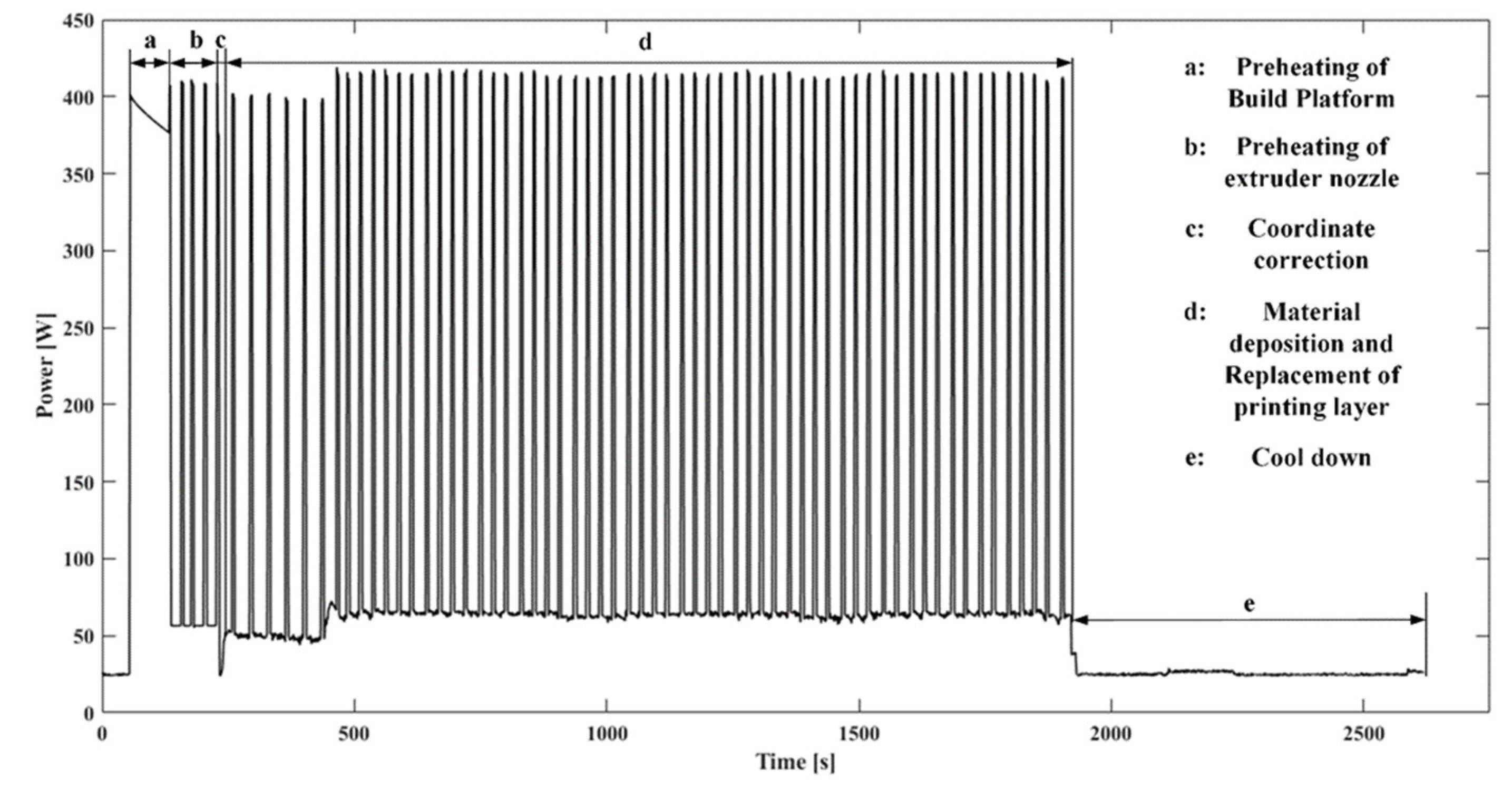
The total power curves of case 1 are shown in Figure 15, wherein stage a represents the heating platform preheating, stage b represents the nozzle preheating, stage c represents the coordinate calibration sub-process, stage d represents the printing stage (including material deposition and layer change), and stage e represents the cooling down sub-process after finishing printing the part.

Table 8. The comparison between measured and predicted values of time and energy consumption.

	Phases	Model
		1			2			3
		Measured	Predicted	Error (%)	Measured	Predicted	Error (%)	Measured	Predicted	Error (%)
Time (s)	a	82	85.9	4.76	132	134.51	1.90	87	89.23	2.56
	b	92	94.18	2.37	98	98.44	0.45	90	92.45	2.72
	c	24	24	0	26	24	7.69	23	24	4.35
	d	1668	1317.57	21.01	1677	1300.35	22.46	17,940	15,223.26	15.14
	e	699	759.58	8.67	1076	900.31	16.33	730	759.58	4.05
	Total	2565	2281.23	11.06	3009	2457.61	18.32	18,925	16,188.52	14.46
Energy (Wh)	a	8.6284	9.15	6.05	14.03	13.89	1.00	9.18	9.48	3.27
	b	3.1077	3.56	14.55	3.94	3.65	7.36	2.89	3.49	20.76
	c	0.6035	0.86	42.50	0.75	0.84	12.00	0.84	0.86	2.38
	d	56.153	49.90	11.14	67.56	48.34	24.90	617.67	575.74	6.79
	e	4.838	5.13	6.04	7.66	6.08	20.63	5.41	5.13	5.18
	Total	73.3306	68.6	6.45	90.75	72.8	19.78	635.87	592.63	6.49

compares measured and predicted values of time and energy consumption data in each stage of case 1. The calculation formula for the prediction error is as follows:

$$\mathrm{Error}=\frac{\left|\mathrm{Measured} \mathrm{value} - \mathrm{Predicted} \mathrm{value}\right|}{\mathrm{Measured} \mathrm{value}}$$

(18)

As can be seen in Table 8, the time error between the predicted value and the measured value calculated by the time model of platform preheating stage (stage a) and nozzle preheating sub-process (stage b) was small for all cases, within 5%. The time error for the coordinate calibration sub-process (stage c) was related to the distance between the nozzle and the origin of coordinates before printing. Before coordinate calibration, if the nozzle was not located at the origin of coordinates, the driving motor would move the nozzle to the vicinity of the origin before calibration. Therefore, the time error in this stage varied largely. In the part printing stage (stage d), the difference between the predicted time and the measured time was more than 15%, and the measured time was greater than the predicted time. This is a fairly normal outcome, because this model only considers the time of the nozzle moving with printing material in addition to the time of the nozzle moving without printing material. The time of the nozzle moving without printing material has a close relation to the scanning strategy. Moreover, in the moving process of the nozzle, the prediction model assumes that the nozzle moves at a uniform speed; but the nozzle accelerated from 0 to the target speed, and then slows down from the target speed to 0 after the current line segment is printed in the actual printing process. In addition, the volume of a single-layer outer wall and an inner wall was assumed to be approximately equal when the prediction model calculated the partial filling of part wall, which made the model produce certain errors in predicting the printing time of thin-walled parts. The error in the cooling sub-process (stage e) between the prediction value and the measured value can be interpreted as follows: the cooling curve of the platform was measured under the condition that there were no parts attached to the platform, and the heat dissipation area of the platform in this state was equal to the surface area of the platform. When printing different models, the area glued to the bottom of the part and the heating platform was affected by the shape and placement of the part, which changed the size of the heat dissipation area of the heating platform. Hence, it affected the heat dissipation rate of the platform substrate and cause time errors. The error between the overall time prediction model and the measured data was 10–20%, which is acceptable.

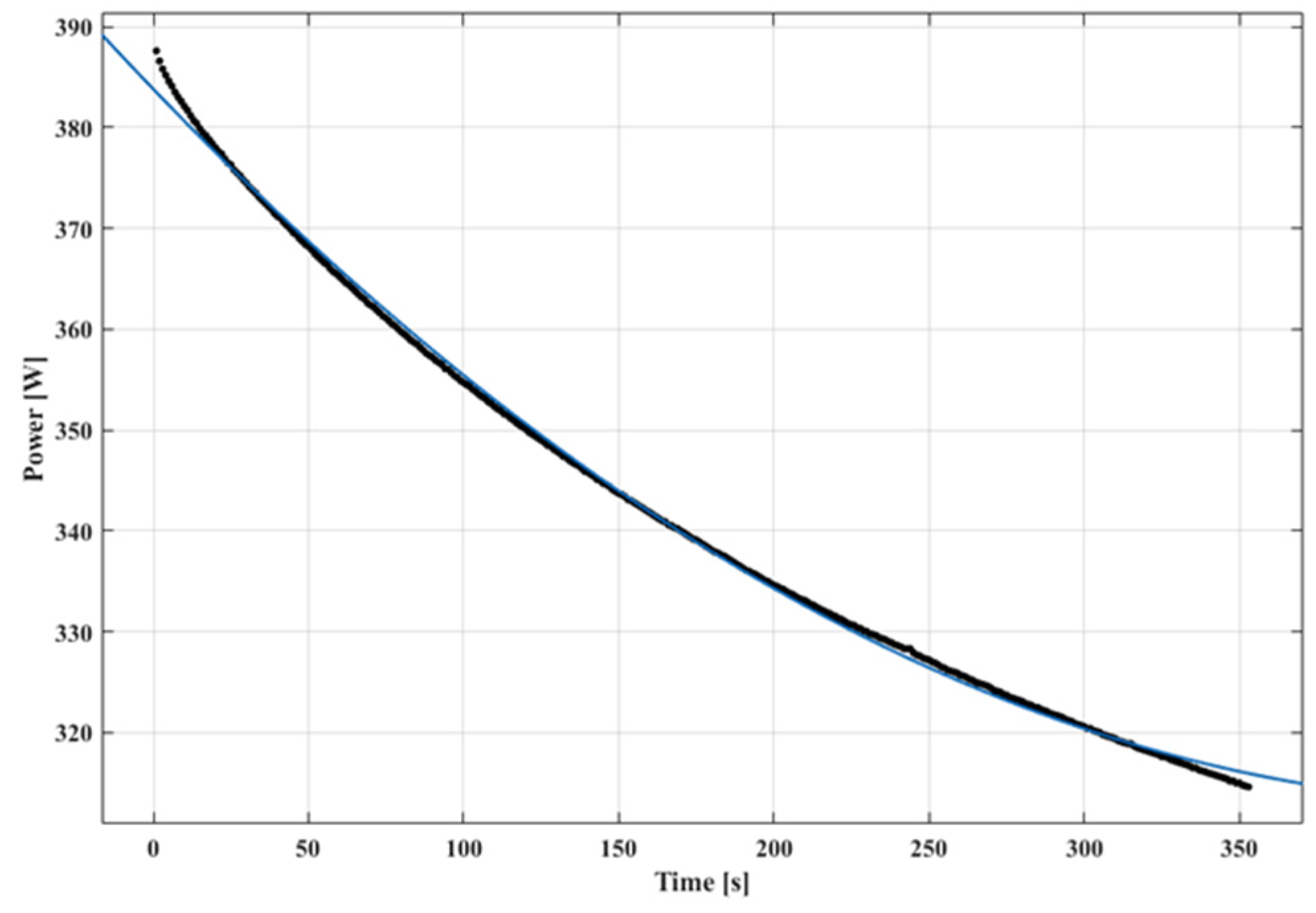
The energy consumption prediction error between the predicted value and the measured value of the platform preheating stage (stage a) was less than 10% for cases (1)–(3). The error came on the one hand from the time prediction error, and, on the other hand, it was due to the approximation of the preheating platform stage heater power curve as a straight line. In addition, taking the heating power of the heating platform as a fixed value was another source of error. The energy consumption error in the nozzle preheating stage (stage b) and coordinate calibration stage (stage c) fluctuated in a wide range. This is because the nozzle preheating stage and coordinate calibration stage lasted a short time, and the heater of the heating platform was the main power-consuming component during this time. The energy consumption errors of the predicted value and measured value in the printing stage (stage d) for cases (1)–(3) were 11.14%, 24.9% and 6.79%, respectively. The energy consumption errors in case (1) and case (3) in stage d were smaller than that in time prediction, while the energy consumption error in case (2) was larger than that in time prediction. The energy consumption errors in the cooling down stage (stage e) were 6.04%, 20.63% and 5.18% respectively. In the cooling down stage, only the control module and LED were in a working state. The energy consumption error in this stage mainly came from the difference between the predicted time and the actual time. In terms of the total energy consumption error, the total energy consumption error in case (1) and case (3) was smaller than the total time error, and the total energy consumption error in case (2) was larger than the total time error, which was similar to the error in the printing stage (stage d). The prediction accuracy of the total energy consumption of each model could reach 93.55%, 80.22% and 93.51%, respectively.

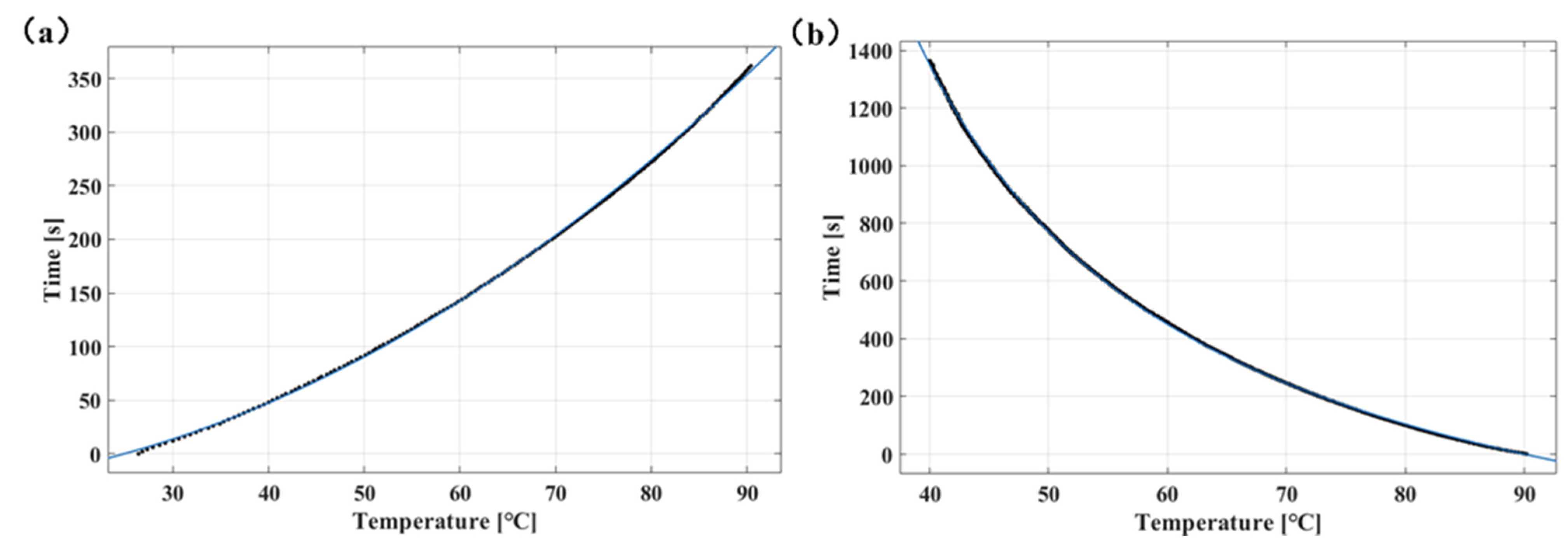
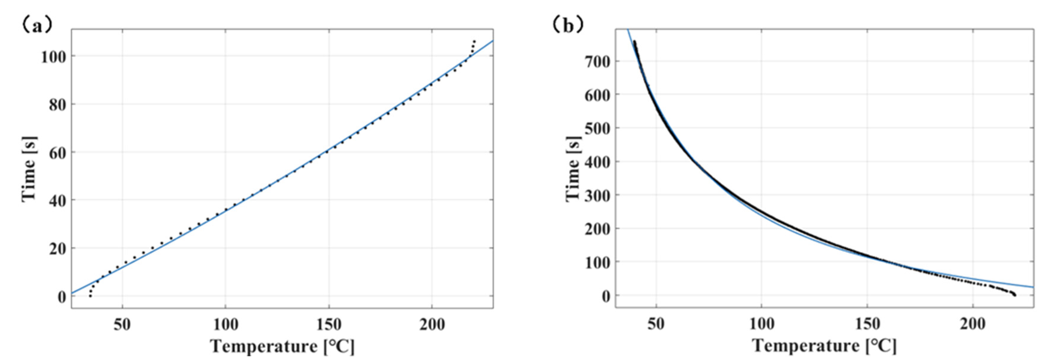
The percentage of each subsystem’s time consumption of the total time is represented in Figure 16, where case (1) and case (2) are small parts with small volumes, while case (3) had medium and large parts. It can be seen that the time required by the printing stage of a part accounted for more than 50% of the total time. Compared with case (2), case (1) had more volume and surface area, but the printing speed and layer thickness of case (2) were both smaller than those of case (1). Therefore, similar manufacturing time was required for case (1) and case (2). Although case (1) and case (3) had the same printing parameters, such as filling speed and filling density, there was a nearly 40% difference in the time required, due to the large volume-difference between case (1) and case (3). Therefore, it can be concluded that the time required for the printing stage changes greatly with changes in the part’s volume, the filling density, printing speed and layering thickness. In addition, the time consumption of the heating platform preheating sub-processes, nozzle preheating process, coordinating the calibration process and the time for layer change were less than 5% of the total time consumption. Although the time consumption of the coordinating calibration processes of the position of the nozzle and platform before the start of printing were closely related to the initial position, the maximum time required by the calibration sub-process was determined by a fixed value, the size of the working space of the machine. The difference between the maximum and minimum required times of the sub-process was about 60 s, and changes in the required time of the calibration sub-process had little influence on the whole printing process. Similarly, variations in the time demand during the platform preheating stage and nozzle preheating stage can be analyzed by looking at Figure 9 and Figure 12. When PLA material is used for printing, the recommended temperature of the platform is 45~60 °C, and the difference in the heating time is about 80 s. The recommended temperature of the nozzle is 190~230 °C, and the difference in the heating time is about 25 s. When ABS material is used for printing, the recommended temperature of the platform is 90~110 °C, and the difference in the heating time is about 180 s. The recommended temperature of the nozzle is 220~260 °C, and the difference of the heating time is about 25 s. The influence of the time variation in the preheating stage on the total printing time decreased with the increase in the total time required. Although the time required in the cooling stage was relatively long, since the time required in the cooling sub-process as only related to the temperature of the platform at the beginning of cooling and the temperature at the end of cooling, the value of the time required in this stage did not vary greatly. The initial and target temperatures of the cooling stage in case (1) and case (3) were consistent, but due to the influence of heat dissipation, there was a 28% difference when printing the two models. From the above analysis, it can be seen that the printing stage had the greatest influence on the total printing time, and the required time of this stage was affected by the geometric parameters of the parts and the setting of printing process parameters.

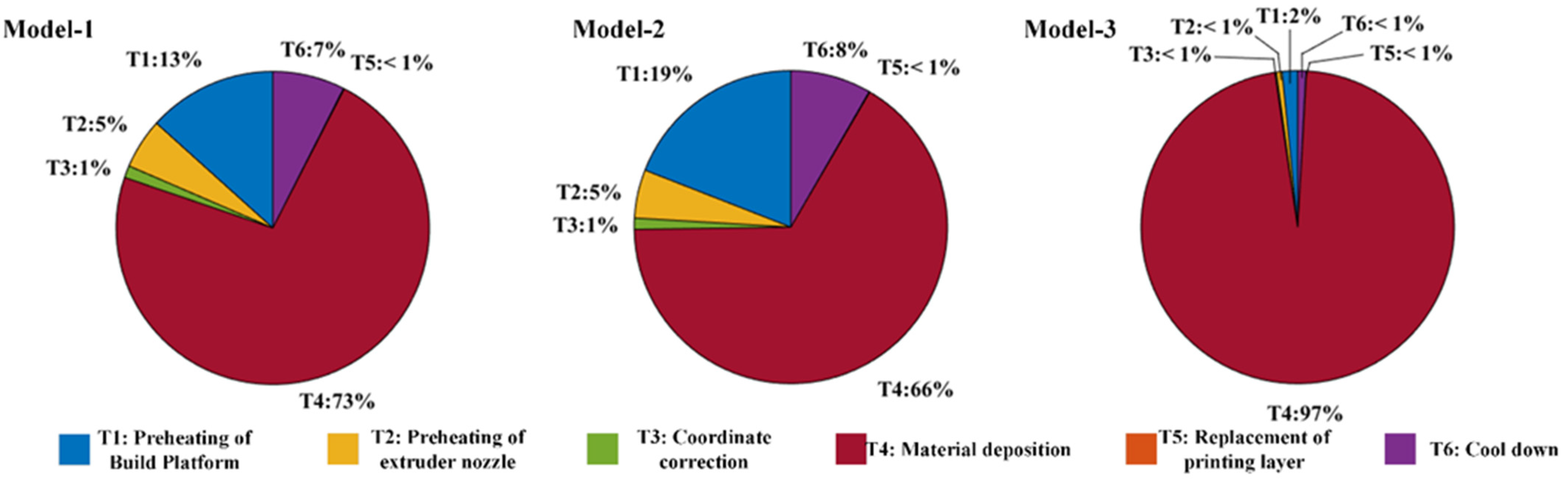
The percentage of energy consumption for each subsystem in the FDM printing process is shown in Figure 17. It can be found that, compared with the smaller time proportion of the platform heating sub-process in the printing process of model (1) and model (2), the energy consumption of this sub-process could reach 13% and 19% of the total energy consumption, respectively. In addition, the energy consumption in the cooling down process was reduced by 26% and 29% compared to the time proportion, respectively. However, the energy consumption proportion increased compared to the time consumption proportion in the printing stage. This is because, in the FDM printing process, electric energy is mainly used to heat the platform and maintain the platform’s temperature. Although the duration of the cooling stage was longer than that of the platform preheating stage, only the control subsystem and LED lighting subsystem were in a working state during the cooling stage, and the power of these two systems was only about 10% of that of the platform heater. Therefore, the energy consumption in the cooling stage accounted for less than 10% of the total energy consumption. 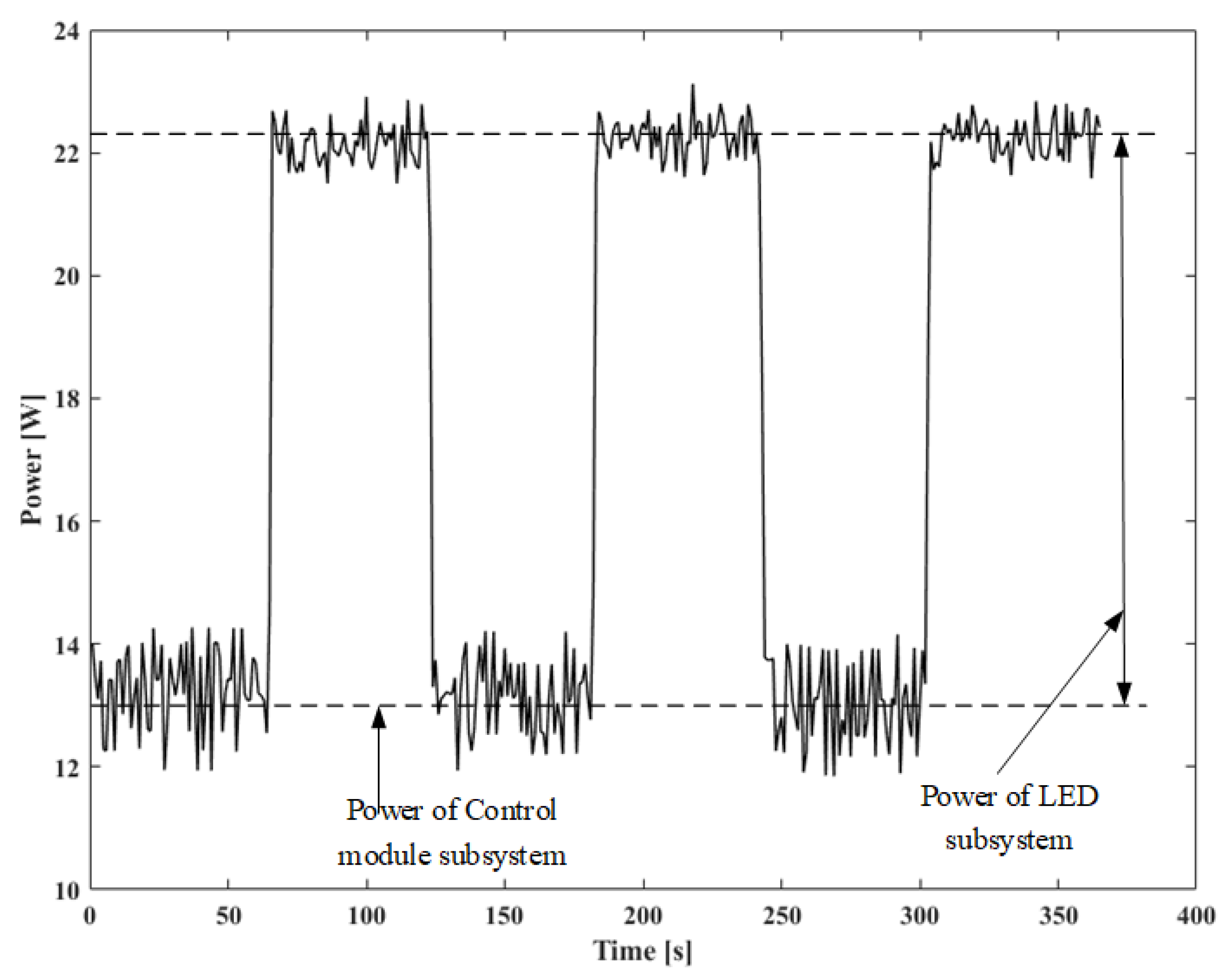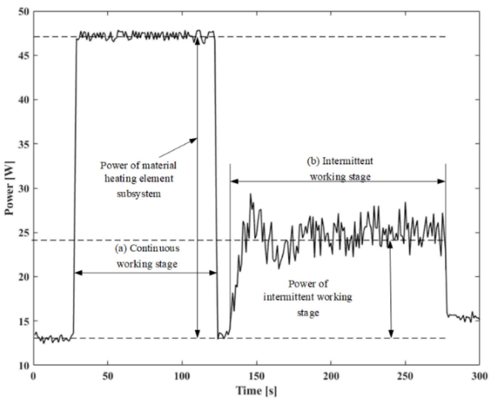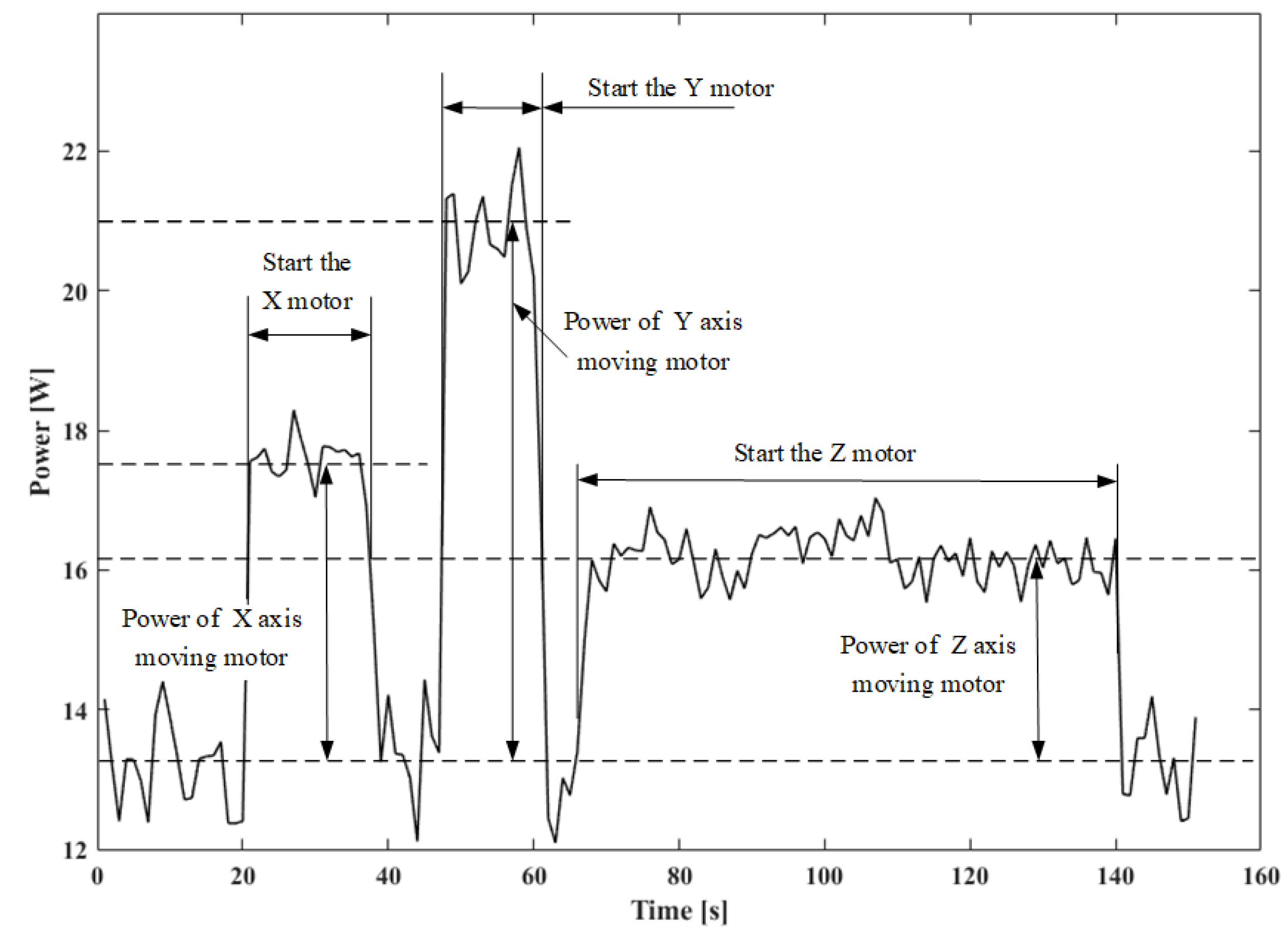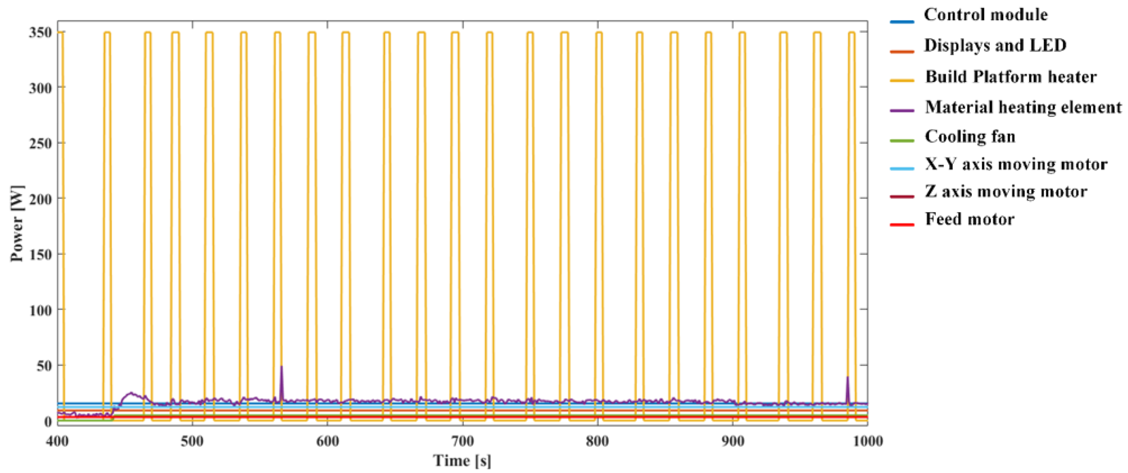Figure 18 represents the power curve of each subsystem in the total process, and it can be found that the transient power value of all subsystems except the platform heater was less than 50 W. The actual running time of the platform heater had the greatest influence on the total printing energy consumption, which was determined by the high power of the platform heater.

5.2. Comparison with Other Methods

There are two methods for the energy prediction of an AM process: SEC models and PPEC models. The SEC model and PPEC model can be expressed as:

$$E=\mathrm{SEC}\times m \mathrm{or} \mathrm{SEC}\times V$$

(19)

$$E={\displaystyle \sum }_i^n{p}_i{t}_i$$

(20)

where E is the total energy consumption, m is the unit mass, V is the unit volume, and $p_i$ and $t_i$ are the power and time consumption of the ith process.

The energy consumption of the FDM process was calculated by the SEC and PPEC models and compared with the measured values. The prediction accuracy (PA) was calculated as follows:

$$\mathrm{PA}=\left(1-\frac{\left|E_{measured}-E_{predicted}\right|}{E_{measured}}\times 100\%\right)$$

(21)

where $E_{predicted}$ and $E_{measured}$ are the predicted and measured energy consumption, respectively. The power values of the FDM components used for the PPEC model comparison are shown in

Table 9. Power of FDM components (from reference [23]).

Units.	Power (W)
Platform warm-up	360
Maintaining the plate temperature	110
Nozzle warm-up	40
Maintaining the nozzle temperature	17
XY-motors	3
Extrusion motor	3
Z-motor	3
Auxiliary system	45

. The comparison results are shown in

Table 10. Comparison of the prediction accuracy of FDM process.

Models	SEC Value (MJ/Kg)	Prediction Accuracy (%) for Model (1)
SEC models	12.5 (Reference [24])	90.04
PPEC models	-	80.86
Model in our study	-	93.55

. The prediction accuracies of the SEC model and PPEC model were 90.4% and 80.86%, respectively, and the model proposed in this paper outperformed the other models. This could be because the SEC model and PPEC model do not consider the state of the component in each stage during the FDM process.

6. Conclusions

In our study, experimental and theoretical investigations into the energy consumption of additive manufacturing activity were carried out to establish a new energy consumption prediction model—which is the prime task for achieving sustainable and green manufacturing, reducing environmental pressures and increasing enterprise revenue. In addition, FDM was selected to verify the effectiveness of the proposed method. The contributions and findings of this paper can be summarized as follows:

• A new energy consumption prediction model was established to forecast the energy consumption of additive manufacturing easily and accurately.
• Three models were studied to verify the effectiveness of this model, and the prediction accuracy was better than the SEC and PPEC models.
• The proposed method considers the working state of each component in the printing process, which promotes its prediction accuracy.
• In virtue of this model, the printing time and energy consumption can be easily predicted. It is convenient for visualization and integration into corresponding software, and provides reference for collaborative optimization of quality and energy consumption.

The prediction model proposed in this paper has some limitations. In the printing stage, the prediction model did not take into account the time required by empty travel and acceleration and deceleration in the nozzle’s movement. The working time of a heater is closely related to the set temperature, the ambient temperature and the adhesion area of the parts, which need be further analyzed. Future work will be conducted to study the relationships between the working characteristics of the heater at the heat preservation stage of the platform and the set temperature and adhesive area. In addition, parsing G-code to analyze power consumption and integrating it into software will be another future work.

References

1. Peng, T.; Kellens, K.; Tang, R.; Chen, C.; Chen, G. Sustainability of additive manufacturing: An overview on its energy demand and environmental impact. Addit. Manuf. 2018, 21, 694–704. [Google Scholar] [CrossRef]
2. Hopkins, N.; Jiang, L.; Brooks, H. Energy consumption of common desktop additive manufacturing technologies. Clean. Eng. Technol. 2021, 2, 100068. [Google Scholar] [CrossRef]
3. Jia, S.; Yuan, Q.; Lv, J.; Liu, Y.; Ren, D.; Zhang, Z. Therblig-embedded value stream mapping method for lean energy machining. Energy 2017, 138, 1081–1098. [Google Scholar] [CrossRef] [Green Version]
4. Jia, S.; Yuan, Q.; Cai, W.; Lv, J.; Hu, L. Establishing prediction models for feeding power and material drilling power to support sustainable machining. Int. J. Adv. Manuf. Technol. 2019, 100, 2243–2253. [Google Scholar] [CrossRef]
5. Zhu, Y.; Peng, T.; Jia, G.; Zhang, H.; Xu, S.; Yang, H. Electrical energy consumption and mechanical properties of selective-laser-melting-produced 316L stainless steel samples using various processing parameters. J. Clean. Prod. 2019, 208, 77–85. [Google Scholar] [CrossRef]
6. Mele, M.; Campana, G.; D’Avino, G. Life cycle impact assessment of desktop stereolithography. J. Clean. Prod. 2020, 244, 118743. [Google Scholar] [CrossRef]
7. Kellens, K.; Mertens, R.; Paraskevas, D.; Dewulf, W.; Duflou, J.R. Environmental Impact of Additive Manufacturing Processes: Does AM Contribute to a More Sustainable Way of Part Manufacturing? Procedia CIRP 2017, 61, 582–587. [Google Scholar] [CrossRef]
8. Gutowski, T.; Jiang, S.; Cooper, D.; Corman, G.; Hausmann, M.; Manson, J.A.; Schudeleit, T.; Wegener, K.; Sabelle, M.; Ramos-Grez, J.; et al. Note on the Rate and Energy Efficiency Limits for Additive Manufacturing. J. Ind. Ecol. 2017, 21, S69–S79. [Google Scholar] [CrossRef]
9. Lv, J.; Peng, T.; Zhang, Y.; Wang, Y. A novel method to forecast energy consumption of selective laser melting processes. Int. J. Prod. Res. 2021, 59, 2375–2391. [Google Scholar] [CrossRef]
10. Lunetto, V.; Priarone, P.C.; Galati, M.; Minetola, P. On the correlation between process parameters and specific energy consumption in fused deposition modelling. J. Manuf. Process. 2020, 56, 1039–1049. [Google Scholar] [CrossRef]
11. Baumers, M.; Tuck, C.; Hague, R.; Ashcroft, I.; Wildman, R. A comparative study of metallic additive manufacturing power consumption. In Proceedings of the 21st Annual International Solid Freeform Fabrication Symposium—An Additive Manufacturing Conference, SFF, Austin, TX, USA, 9–11 August 2010; pp. 278–288. [Google Scholar]
12. Dunaway, D.; Harstvedt, J.D.; Ma, J. A preliminary experimental study of additive manufacturing energy consumption. In Proceedings of the ASME Design Engineering Technical Conference, Cleveland, OH, USA, 6–9 August 2017. [Google Scholar]
13. Paris, H.; Mokhtarian, H.; Coatanéa, E.; Museau, M.; Ituarte, I.F. Comparative environmental impacts of additive and subtractive manufacturing technologies. CIRP Ann. Manuf. Technol. 2016, 65, 29–32. [Google Scholar] [CrossRef]
14. Jia, S.; Cai, W.; Liu, C.; Zhang, Z.; Bai, S.; Wang, Q.; Li, S.; Hu, L. Energy modeling and visualization analysis method of drilling processes in the manufacturing industry. Energy 2021, 228, 120567. [Google Scholar] [CrossRef]
15. Gutierrez-Osorio, A.H.; Ruiz-Huerta, L.; Caballero-Ruiz, A.; Siller, H.R.; Borja, V. Energy consumption analysis for additive manufacturing processes. Int. J. Adv. Manuf. Technol. 2019, 105, 1735–1743. [Google Scholar] [CrossRef]
16. Yang, Y.; Li, L.; Pan, Y.; Sun, Z. Energy Consumption Modeling of Stereolithography-Based Additive Manufacturing Toward Environmental Sustainability. J. Ind. Ecol. 2017, 21, S168–S178. [Google Scholar] [CrossRef] [Green Version]
17. Jia, S.; Yuan, Q.; Cai, W.; Li, M.; Li, Z. Energy modeling method of machine-operator system for sustainable machining. Energy Convers. Manag. 2018, 172, 265–276. [Google Scholar] [CrossRef]
18. Hu, F.; Qin, J.; Li, Y.; Liu, Y.; Sun, X. Deep Fusion for Energy Consumption Prediction in Additive Manufacturing. Procedia CIRP 2021, 104, 1878–1883. [Google Scholar] [CrossRef]
19. Li, Y.; Hu, F.; Qin, J.; Ryan, M.; Wang, R.; Liu, Y. A Hybrid Machine Learning Approach for Energy Consumption Prediction in Additive Manufacturing. In Lecture Notes in Computer Science (Including Subseries Lecture Notes in Artificial Intelligence and Lecture Notes in Bioinformatics); Springer: Cham, Switzerland, 2021; pp. 622–636. [Google Scholar]
20. Yang, Y.; He, M.; Li, L. Power consumption estimation for mask image projection stereolithography additive manufacturing using machine learning based approach. J. Clean. Prod. 2020, 251, 119710. [Google Scholar] [CrossRef]
21. Qin, J.; Liu, Y.; Grosvenor, R. Multi-source data analytics for AM energy consumption prediction. Adv. Eng. Inform. 2018, 38, 840–850. [Google Scholar] [CrossRef]
22. Qin, J.; Liu, Y.; Grosvenor, R.; Lacan, F.; Jiang, Z. Deep learning-driven particle swarm optimisation for additive manufacturing energy optimisation. J. Clean. Prod. 2020, 245, 118702. [Google Scholar] [CrossRef]
23. Ma, Z.; Gao, M.; Wang, Q.; Wang, N.; Li, L.; Liu, C.; Liu, Z. Energy consumption distribution and optimization of additive manufacturing. Int. J. Adv. Manuf. Technol. 2021, 116, 3377–3390. [Google Scholar] [CrossRef]
24. Yi, L.; Chen, T.; Ehmsen, S.; Gläßner, C.; Aurich, J.C. A study on impact factors of the energy consumption of the fused deposition modeling process using two-level full factorial experiments. Procedia CIRP 2020, 93, 79–84. [Google Scholar] [CrossRef]
Figure 1. The universal process of the AM.
Sustainability 14 03757 g001
Figure 2. A schematic diagram of an FDM machine.
Sustainability 14 03757 g002
Figure 3. The (a) straight-line and (b) zig-zag filling strategies.
Sustainability 14 03757 g003
Figure 4. The working state of each system at each stage. (The blue part represents the continuous working state, the green part represents the intermittent working state and the white indicates the part is not working).
Sustainability 14 03757 g004
Figure 5. Printed model for model 1–3, where (a) represents the actual parts and (b) represents the sliced model.
Sustainability 14 03757 g005
Figure 6. Experimental equipment: (a) FDM printing machine and (b) power quality analysis.
Sustainability 14 03757 g006
Figure 7. Power curves for control module subsystem and LED subsystem.
Sustainability 14 03757 g007
Figure 8. Power curves of the printing platform heater subsystem.
Sustainability 14 03757 g008
Figure 9. Temperature–time curves for (a) preheating platform stage and (b) cooling stage.
Sustainability 14 03757 g009
Figure 10. The power–time curves for heating the platform in the preheating platform stage.
Sustainability 14 03757 g010
Figure 11. Power curves of the platform heater subsystem.
Sustainability 14 03757 g011
Figure 12. Time–temperature curves of the nozzle in the (a) preheating stage and (b) cooling down stage.
Sustainability 14 03757 g012
Figure 13. Power–speed relationship curve of the cooling fan for (a) measured curve and (b) fitted curve.
Sustainability 14 03757 g013
Figure 14. Power curves of moving motor in the X, Y and Z axes.
Sustainability 14 03757 g014
Figure 15. Power curves of case 1.
Sustainability 14 03757 g015
Figure 16. The percentage of time consumed by each sub-process in total time.
Sustainability 14 03757 g016
Figure 17. Percentages of sub-process energy consumption of total energy consumption.
Sustainability 14 03757 g017
Figure 18. Power curve of each subsystem in total process.
Sustainability 14 03757 g018