1. Introduction
The current global energy system is experiencing an optimization process and aims to increase its use of clean energy, including solar, wind, nuclear, hydro and other renewables. However, this system consisting of diverse energy sources is apt to trigger swings in the power grid. In this case, hydropower, which is superior in terms of rapid startup and shutdown as well as in its effective regulation of power quality, has long had a crucial role in stabilizing the power system.
The runner of a turbine serves as the core of the hydro-energy conversion. It directly determines the stability of the hydraulic system and further obliquely affects the robustness of the electric system. It is thereby essential to optimize the runner-design process and predict its working performance, particularly at the early stage of a hydropower project. For this purpose, experiments [
1,
2] and CFD simulations [
3,
4,
5] are the two widely used technologies. However, satisfactory results require high-end instruments such as Particle Image Velocimetry [
6,
7], Laser Doppler Velocimetry [
8,
9] or Remote Sensing Survey. Likewise, accurate CFD results impose high demands on supercomputers. Consequently, the mathematical-analysis method seems a preferable alternative for overcoming these shortcomings. However, the relevant analytical methods to date have mainly been used for the runner’s inverse design [
10,
11,
12,
13] and seldom for solving the runner’s internal characteristics [
14].
In this ambit, a few studies focused on the direct design of centrifugal pump and its flow analysis [
15,
16]. By extension, the flow on the stream surface (S1) was converted to a 2D Cartesian coordinate system by conformal transformation. The flow around the cascade was further described by equations of integral form, based on which the relative velocity on the blade surface was derived [
17]. In their work, a discrepancy arose between calculations and measurements, presumably attributable to both ignoring the effects of blade shape on the flow and to the unsatisfied momentum equation in the blade channel [
18]. This method was later improved with a direct and inverse iteration, and distributions of the relative and meridian velocities were obtained by solving continuity and momentum equations with the streamline-curvature method [
19,
20].
As for the analytical method in turbines, most studies have only focused on the flow patterns at the runner’s inlet and outlet, particularly on their velocity triangles [
21,
22]. On the meridional plane, the blade of the pump-turbine was discretized and the distributions of Eulerian energy were deduced by a direct and inverse method [
23]. Therein, a surface coordinate was first established on the S1 stream surface of a pump turbine. This decisive step implies the importance of describing flow patterns in the S1-surface coordinate system. Additionally, some relevant technologies have been reported. For instance, spherical coordinates associated with the conformal-transformation method were adopted to investigate the flow in a tubular turbine. The results revealed the relationship between guide-vane opening and the flow at the vane outlet [
24]. Then, the runner blade was discretized in spherical coordinates and further designed with the help of cylindrical coordinates [
25]. Special attention has also been dedicated to the mathematical models describing swirling flow in the turbomachinery [
26] and downstream of the runner [
27,
28]. Then, the helical flow pattern was described by the partial differential function (PDF) of the stream function. This PDF can be solved by converting it to constrained variational problems or under simplified conditions, and then validated by the finite-element method [
29,
30].
Most of these studies tried to determine the direct and inverse design of reaction runners. Few of them obtained the hydraulic characteristics and internal flow field under ideal cases or by the virtue of measurements. Herein, an analytical approach based on the classic runner-design method is introduced, named the analytical method of characteristics (AMOC). This approach focuses on predicting the internal and external characteristics of a Francis turbine without performing extra tests or finite-element simulations; only the runner configuration and its operational parameters are required. In this study, a calculation procedure is performed at the BEP under incompressible and inviscid-flow conditions. This analytical work aims to accurately and effectively predict the optimal hydraulic efficiency and flow field in an existing runner, to quantitatively analyze the energy conversion on the blade and to reveal the pressure difference across the blade.
The paper is organized as follows:
Section 2 presents the main procedures of the AMOC approach, with detailed steps in
Appendix A.
Section 3 takes the form of a case study of a Francis turbine, describing the corresponding results and its validation by the help of the finite-volume method.
Section 4 contains conclusions and outlooks.
2. AMOC Methodology Implementation
2.1. Basic Assumptions
A mathematical model describing the flow in the blade channel is justifiably crucial to analytically determine the runner characteristics. Indeed, real flow is complicated due to its kinematics, dynamics and thermodynamics or even their interactions. In order to simplify this issue and effectively implement the AMOC, some hypotheses are listed as follows:
The liquid is inviscid, single-phase and incompressible.
The flow field in the runner is only subject to kinematics and described based on monistic theory, namely the velocity at a certain point is determined only by the streamwise distance from the origin of a streamline.
The fluid flows smoothly in the blade channel, i.e., the relative velocity component is aligned with the local tangential direction of the relative spatial streamline.
2.2. Implementation Procedures
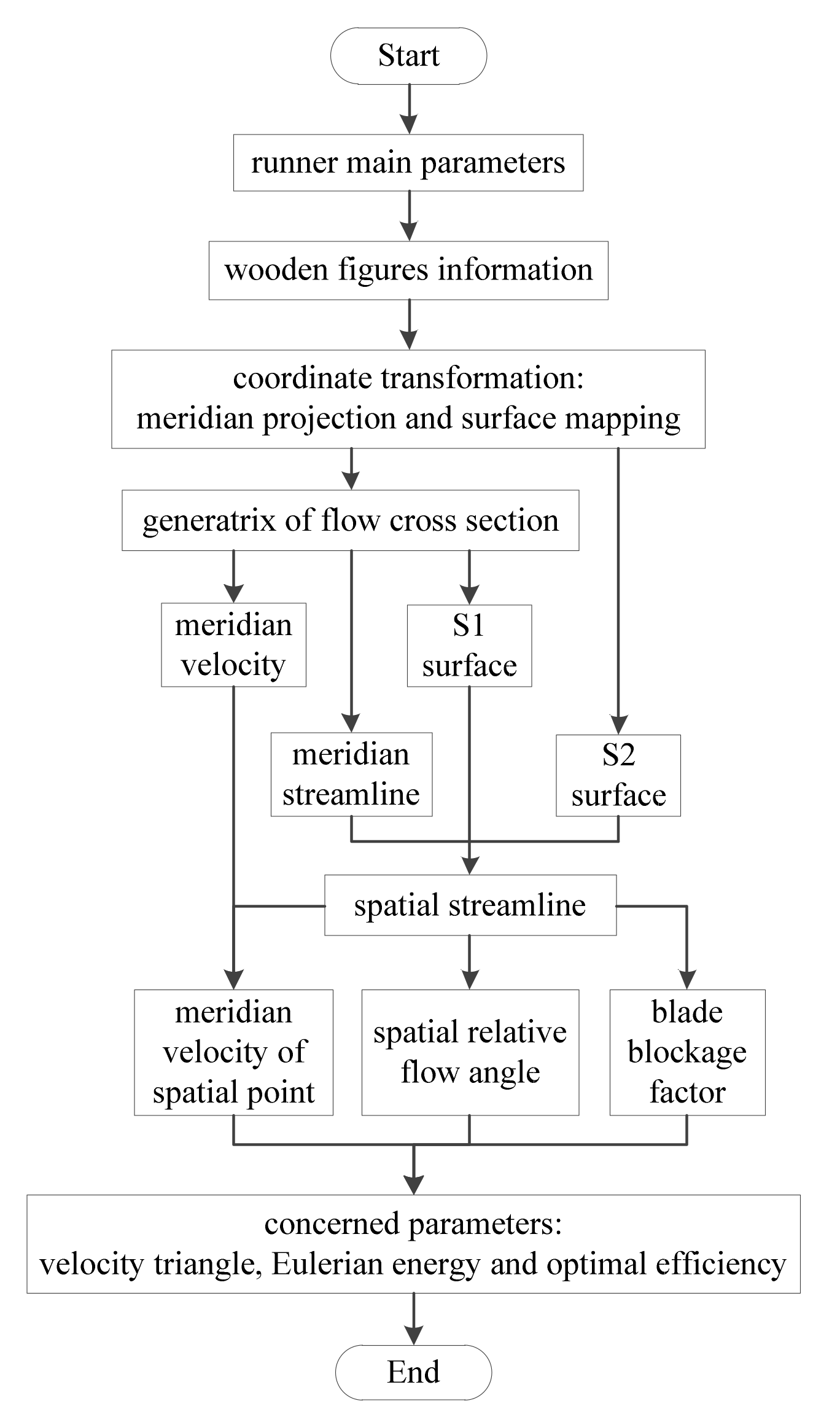
The implementation procedure of the AMOC approach is illustrated in
Figure 1. This approach is based on the well-known classical-design theory of radial-axial turbine runners under incompressible and inviscid-flow conditions. The three-dimensional runner configuration, particularly the spatial blade channel, is discretized and projected onto the meridional plane. Closely following this, spatial streamlines are formed by the interaction of the blade and the stream surface. Then fluid kinematic relationships are constructed for each streamline and later the kinematic parameters are solved.
Furthermore, the flow at the blade-channel inlet is irrotational, with uniform radial and tangential velocity components. However, at the outlet of the channel, a uniform axial-velocity profile is considered. A blade-blockage factor is introduced in order to account for the effects of blade thickness. Some parameters are initially input in order to perform this approach, including:
A model of the runner and the main geometry of the blade, such as wooden figures.
Meridional channel geometry, such as the crown, band, and blade leading-edge and trailing-edge curves.
The operational parameters at the BEP, such as available unit speed, head, and discharge.
Finally, the approach outputs several spatial streamlines and their relevant parameters including the velocity components, Eulerian energy, absolute flow angle, relative flow angle, runner’s hydraulic efficiency and pressure difference over the blade.
The general descriptions of
Figure 1 are presented as follows with additional details on the derivation shown in
Appendix A.
2.2.1. Coordinate Transformation
Meridian projection and surface mapping are performed in this section. Geometries described in a Cartesian system are converted into a curved coordinate system by virtue of the stream surface (S1) and the blade-chamber surface (S2). Detailed deviations can be found in
Appendix A.1. The coordination operations are defined by Equations (A1)–(A4).
2.2.2. Generatrix of Flow Section and Meridional Velocity
The cross section of the flow in the blade channel is perpendicular to the S1 stream surface by the classical design theory of radial-axial turbine runners. Its intersection with the meridian plane generates the so-called generatrix, which can be geometrically acquired by inserting inscribed circles in the blade channel. As shown in
Figure A3, one generatrix, the arc
derived from Equation (A5), rotates round the
Z-axis to form the flow cross section. Then the meridional velocity is computed in
Appendix A.2.
2.2.3. Streamline Cluster Generation
Meridional streamlines discretize the flow channel into several passages, with each passage conveying the same discharge. These meridional streamlines (SL) and ten relative spatial streamlines (SSL) are derived by the steps in
Appendix A.3.
Appendix A.4 elaborates the steps to determine the relative flow angle at each node on the spatial streamlines. Then, with the known meridional velocity of the SL, the corresponding meridional velocity on the SSL is derived in
Appendix A.5. Blockage effects due to the blade thickness are taken into account by Equations (A15) and (A16).
Using the above procedures, all of the parameters with which to further implement the AMOC are obtained, including the revised meridional velocity Vm′, the relative flow angle βi and the blockage factor 1/ki at each node on the SSL.
By recalling the Law of sines and Law of cosines, the velocity components are derived from Equations (A17) to (A21).
Afterwards, the Eulerian energy at each node on the SSL is quantified as:
where
EUi denotes the Eulerian energy at node
i.
Recalling the fundamental equation of a hydraulic turbine defined as the integral form [
28]:
where
S1 and
S2, respectively, denote the cross sections upstream and downstream of the runner.
This equation defines the change in flux of the moment of momentum along both the streamwise and spanwise directions. According to the second assumption in
Section 2.1, this equation is integrated as:
then, the runner hydraulic efficiency can be computed where,
γ is the liquid unit weight and
g is the gravity acceleration.
EUb1 and
EUb2 separately denote Eulerian energies at the blade inlet and outlet.
H0 is the rated head and
ηr0 is the runner’s hydraulic efficiency at the BEP as computed by the AMOC.
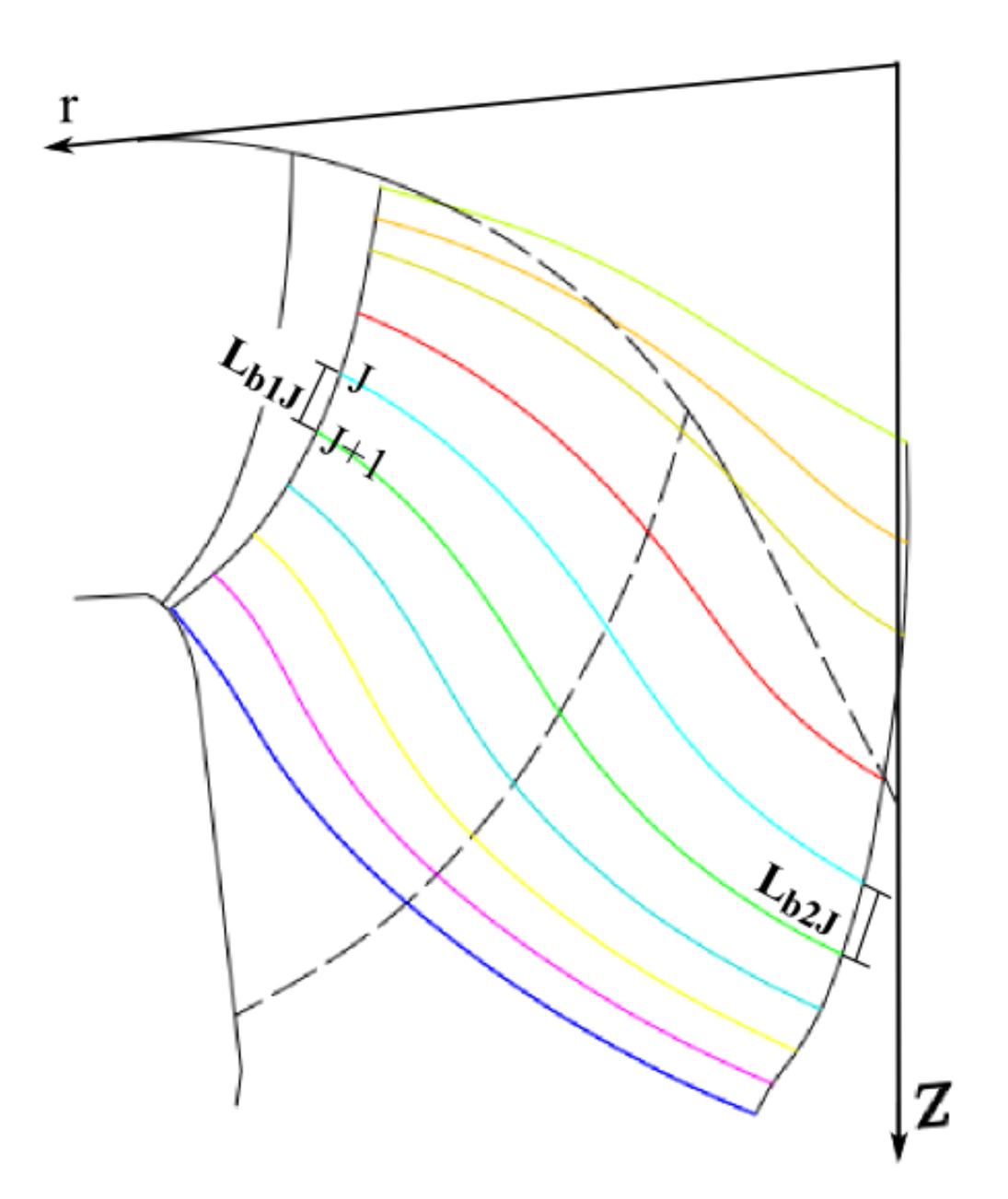
Figure A5 shows the discretization of the blade inlet and outlet, as well as the notation of each subsection. With the length-weighted method, the Eulerian energy in Equation (3) is therefore replaced by the average value, quantified as:
where
where
where
J denotes the ordinal of the SSL.
J = 1, 2, …, 9 due to ten SSLs derived here as shown in
Figure A4. The subscript
b1 and
b2 denote blade inlet and outlet separately.
denotes the length-averaged Eulerian energy.
EUJ denotes the Eulerian energy on the
Jth SSL.
LJ denotes the length of the subsection.
ξJ denotes the weighted factor of each segment.
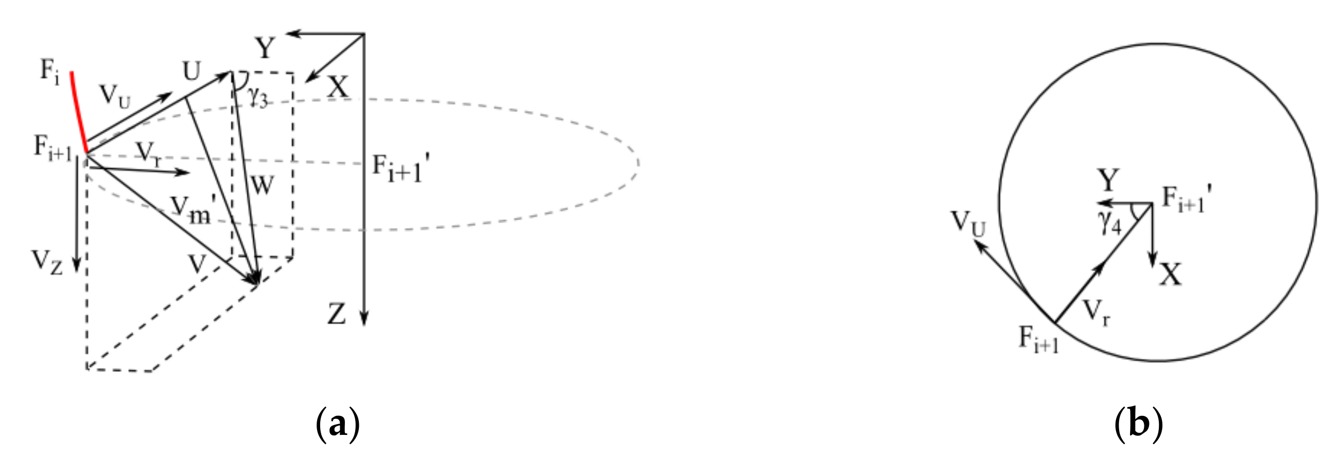
2.3. Transformation of Velocity Component
The velocity components are converted from velocity triangles to the Cartesian system by vector operation and coordinate operation in
Appendix B. Then, the absolute streamlines are derived by interpolation and extrapolation.
3. Case Study and Results Discussion
3.1. Basic Parameters of Runner Model
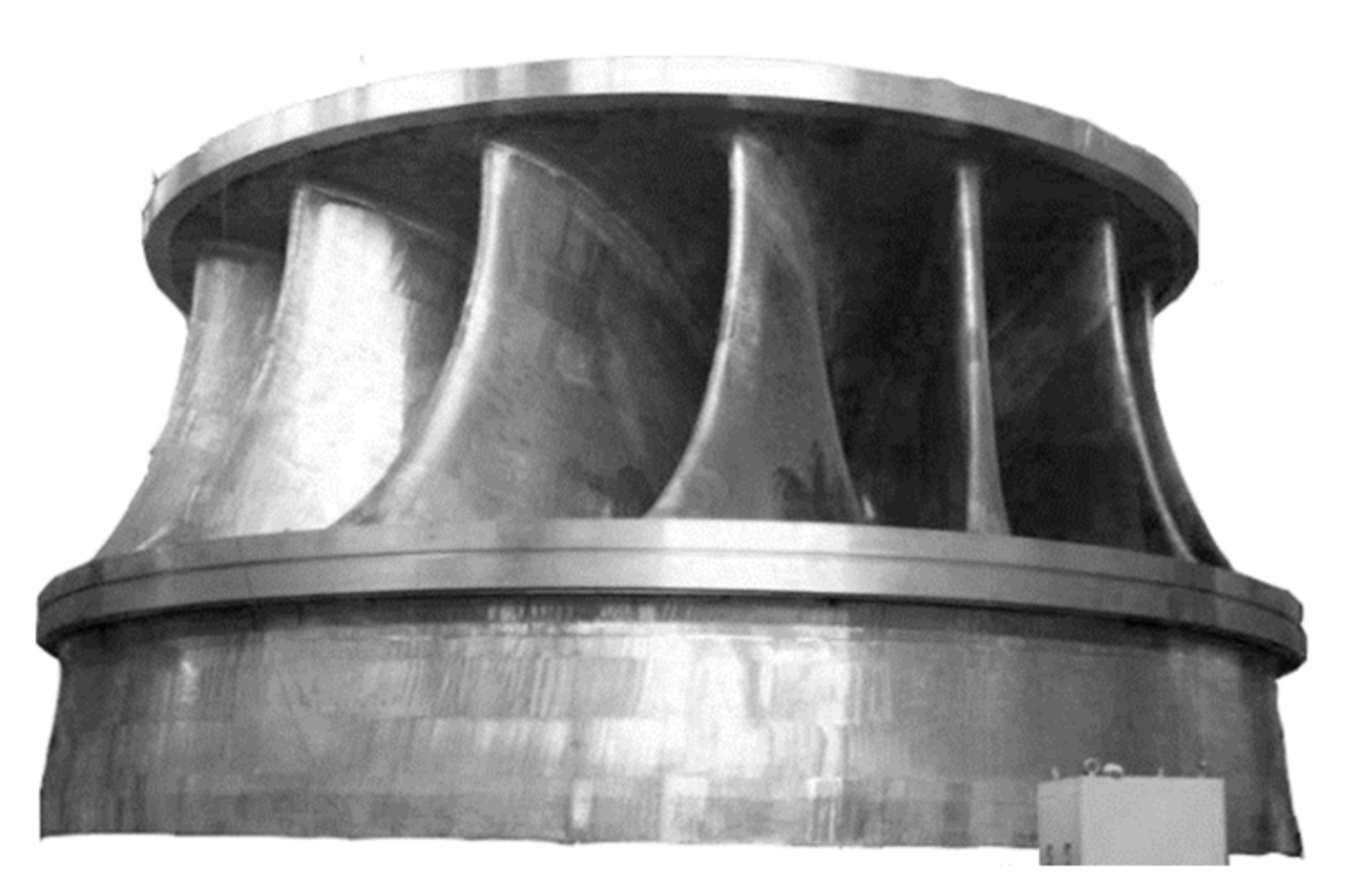
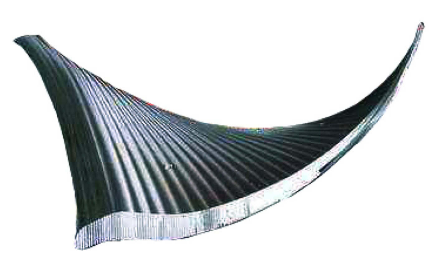
This AMOC procedure was performed on a Francis turbine model (A858a-36.6) with an X-shaped blade that was conceptualized and developed by Prof. Hermod [
31,
32]. A prototype of this model serves at the Three Gorges right bank station. Corresponding runner and blade illustrations are separately presented in
Figure 2 and
Figure 3. The main dimensions of this model and its operational parameters at the BEP are tabulated in
Table 1. The X-blade runner features a twisted blade and a negative angle at the inlet in order to reduce the cross flow in the blade channel [
32]. These features make the second and third assumptions more reasonable.
3.2. Validation and Result Analyses
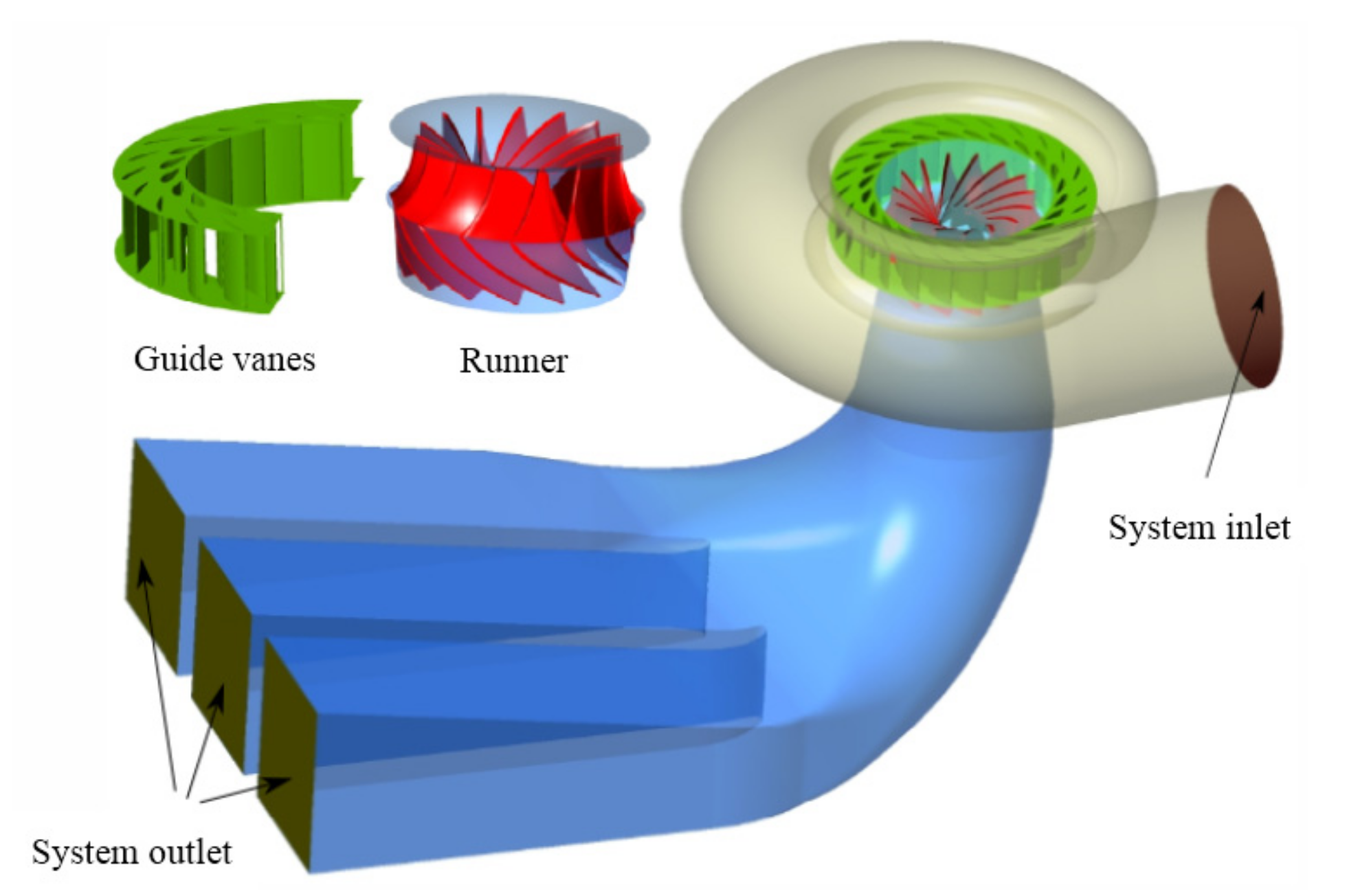
With respect to the same turbine model, the results predicted by the AMOC approach were evaluated by experimental data and using the CFD software ANSYS Fluent 19.2. In the numerical simulation, the three-dimensional model and flow passage are illustrated in
Figure 4. This system consisted of the spiral case, guide vanes, runner and draft tube. A grid with two million elements was employed to the whole domain. Then, the Navier–Stokes equations coupled with the
k-ε turbulence model were solved in the steady state. A total head of 30 m was prescribed at the system inlet, and an average static pressure of 0 Pa was used at the system outlet. This simulation configuration has been widely used in the field of hydraulic turbomachines. Simulation results have shown good agreement with experiments [
10,
33], at least at the BEP. A ThinkPad laptop T460p was used to perform the simulation, and it took almost twelve hours to get satisfactory results for one operation point.
3.2.1. Time Consumption and Turbine Hydraulic Efficiency
By performing the AMOC, the whole implementation process consumed around two hours to obtain all of the desired results using an identical laptop. From this point, the time consumption of AMOC was 1/6 of the CFD calculation. Here, the efforts of 3D modeling were not taken into account, let alone the various cases throughout the whole operation range.
Part of the data report obtained at the blade inlet and outlet after running the AMOC is listed in
Table 2, including various components of the velocity triangles, Eulerian energy, the length of each subsection and the optimal hydraulic efficiency computed from Equation (1) to Equation (5). That is,
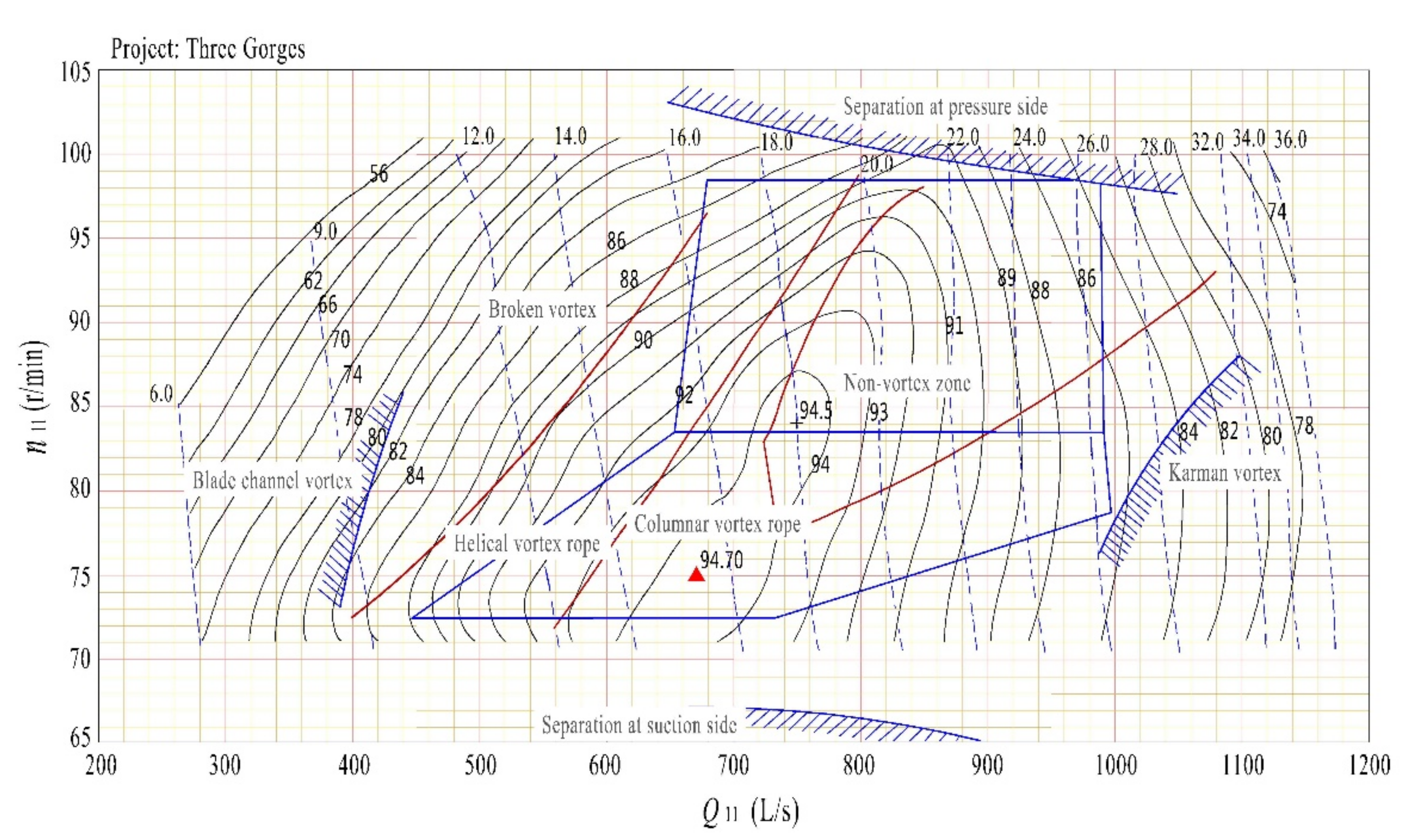
This turbine model was tested by the Harbin electrical-machine factory in China. The main results used to validate the analytical approach are shown in
Table 3 [
34]. The optimal efficiency derived from the test was 94.63%. This value in the runner hill chart is 94.7% as illustrated in
Figure 5 [
35]. Moreover, the optimal hydraulic efficiency of the runner predicted by the Navier–Stokes solver is 94.57%. The efficiency value computed by the different methods are compared in
Table 4. The relative errors are calculated, and these minor discrepancies quantitatively validate that the AMOC enables the accurate prediction of the runner’s optimal hydraulic efficiency. Admittedly, the experimental value of the efficiency was calculated between the cross sections upstream of the runner and downstream of the runner, and this value takes into account the hydraulic efficiency, the mechanical efficiency and the volumetric efficiency, respectively, whereas the analytical approach in this paper predicts only the hydraulic efficiency from the blade inlet towards the outlet. At the BEP, the mechanical and volumetric loss is negligible, which leads to a good agreement between the experimental and the analytical approaches.
3.2.2. Velocity Distribution in Blade Channel
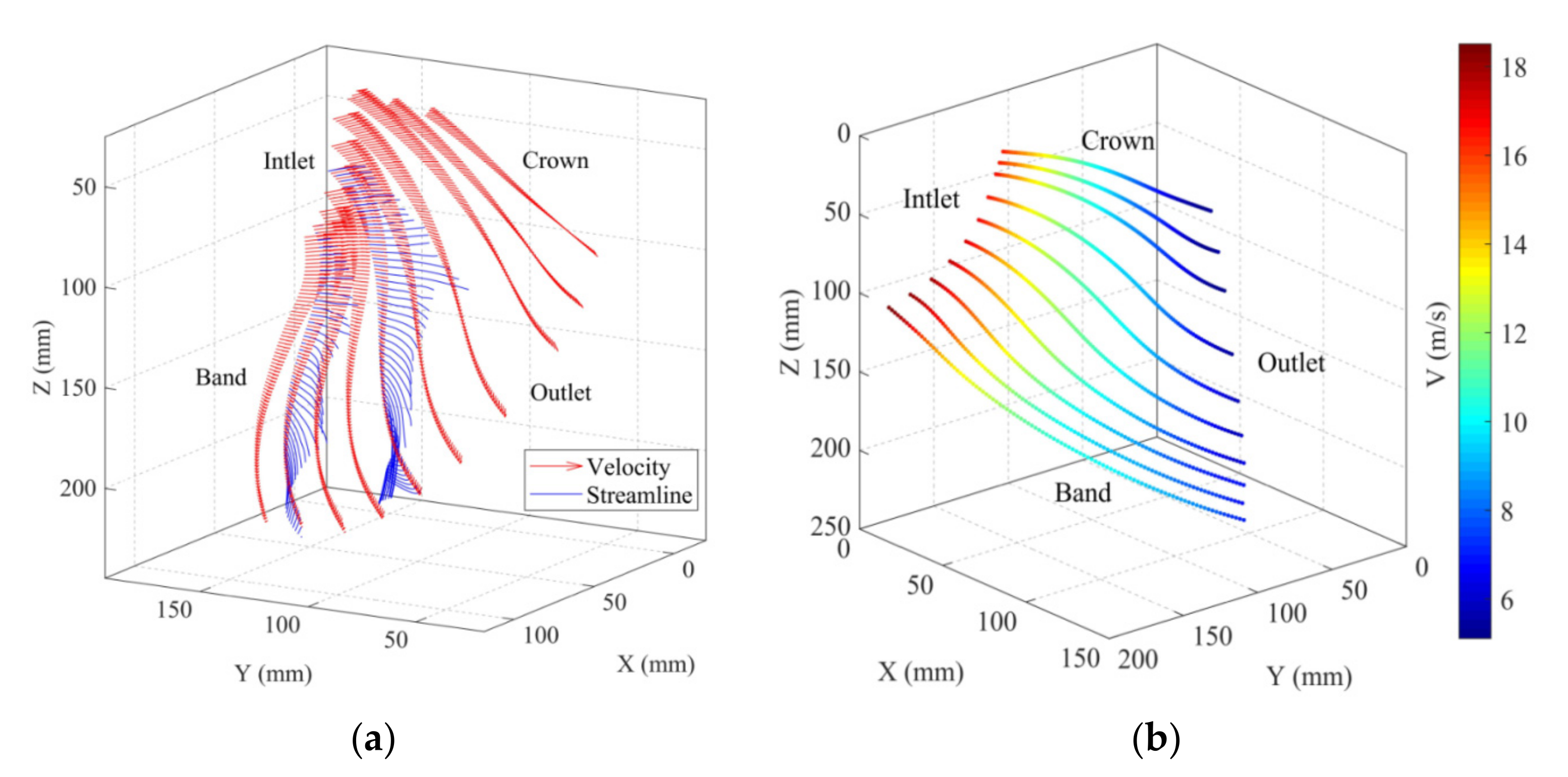
By data processing and velocity conversion, many more visual illustrations are presented.
Figure 6 shows both the vector and scalar of the absolute velocity along the SSLs. Additionally, the absolute streamlines are partially plotted in the left figure by blue lines. It is evident that the radial flow gradually transfers to the axial direction due to the blade configuration. The meridional velocity correspondingly tends to perform in the same manner along the SSL. The runner additionally rotates clockwise. Therefore, the direction of absolute velocity evolves, namely being horizontal to the right at the blade inlet and inclined downwards at the outlet, as demonstrated by the blue lines in
Figure 6a. This pattern greatly depends on the runner configuration and indeed, the flow features here coincide with the turbine at medium specific speed. Meanwhile, the length of the red arrows represents the magnitude of absolute velocity. Its streamwise evolution implies that the velocity smoothly decreases, which agrees well with the distribution of the velocity scalar in
Figure 6b. Due to the effects of circumferential velocity, the maximum and minimum values separately emerge at the inlet near the band and at the outlet adjacent to the crown. These locations would possibly suffer from large stress, thereby inducing flow separation and other elusive hydraulic turbulence. Overall, in this section, the velocity distributions from the AMOC feature smooth transitions, which is justifiably rational at the BEP.
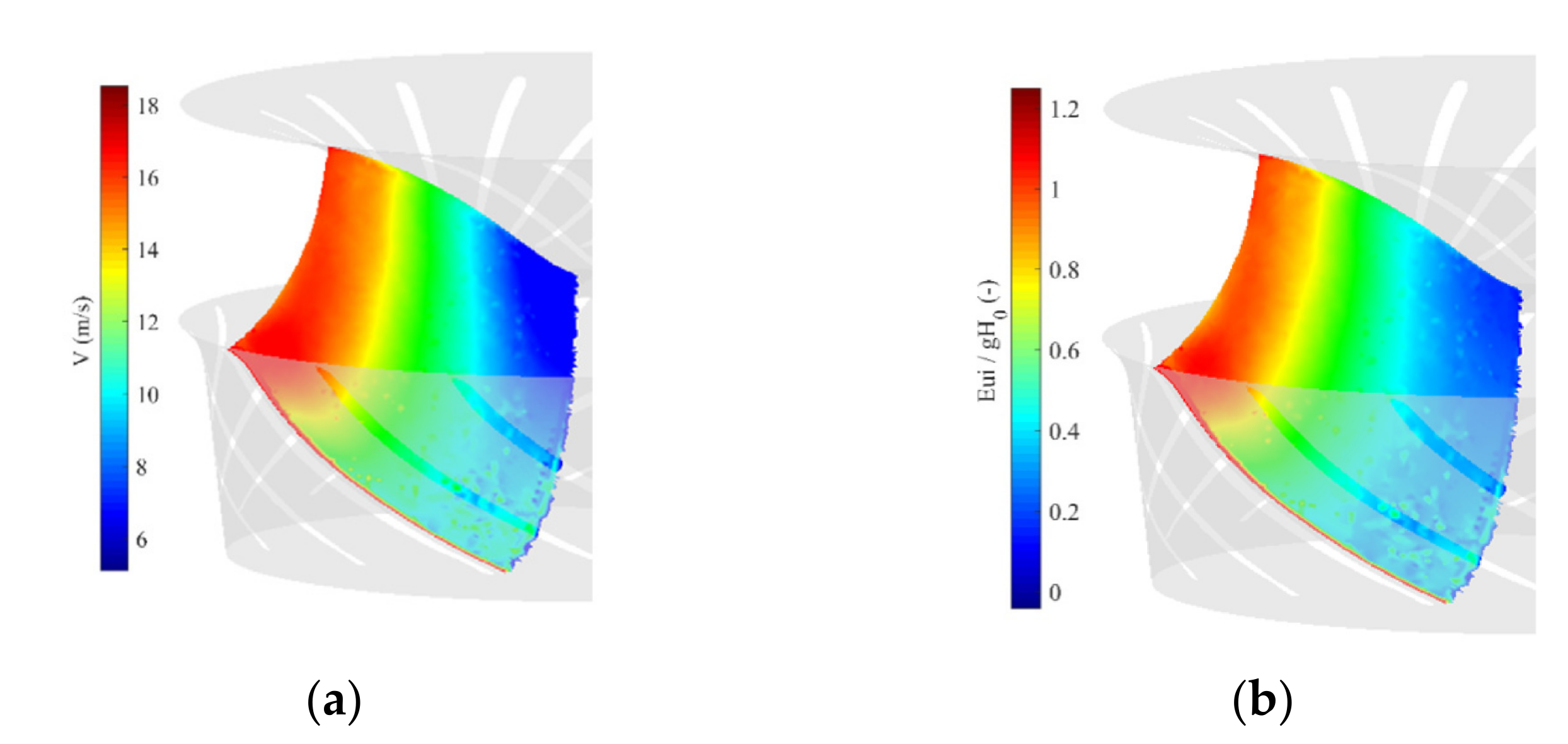
Additionally, the Navier–Stokes solver provides the absolute velocity and Eulerian energy distributing on a certain S2 surface, as shown in
Figure 7. To further aid in the assessment of the results, the runner crown and the band are superimposed onto the flow fields. There is good agreement in the velocity distribution, as evidenced in
Figure 6b and
Figure 7a. The absolute velocity in
Figure 7a smoothly evolves from the blade’s leading edge towards the trailing edge in the same manner as shown in
Figure 6. Therefore, the main flow features and velocity magnitude are well approximated by the AMOC approach, and the S2 surface is basically divided into three parts: red, green and blue. Their boundaries, to some extent, coincide with the blade’s leading and trailing edges. This implies the feature of the X-shaped blade, namely less cross flow from the crown to the band.
3.2.3. Eulerian Energy in Blade Channel
In the (
m,
θ) curved coordinate system, the length of the SSL projection on the m-axis and g
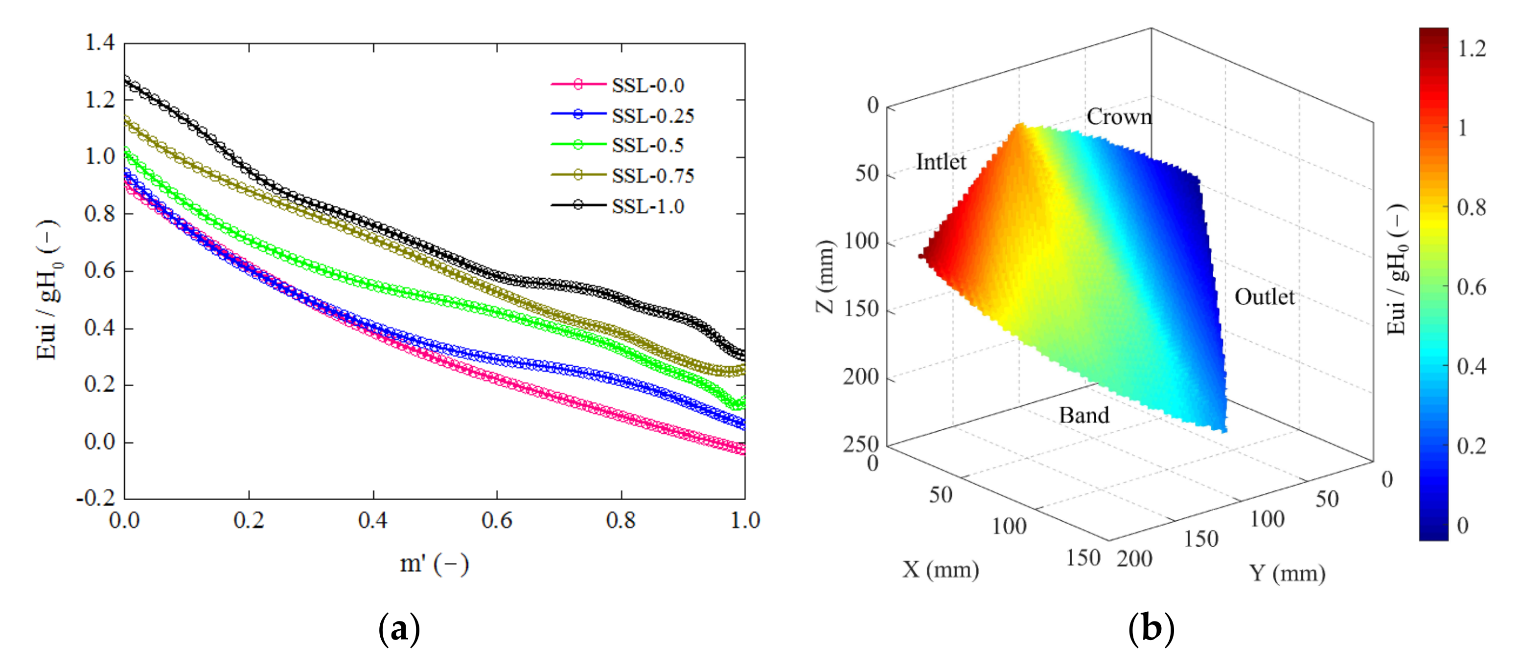
H0 are used to normalize the coordinate and Eulerian energy, respectively, of each point on the corresponding SSL.
Figure 8a displays the resultant distribution of the dimensionless Eulerian energy on five spatial streamlines. The contour of this energy on the S2 surface is illustrated in
Figure 8b. Obviously, Eulerian energy shows both a spanwise ascent and a streamwise descent trend. On the other hand, the fluid potential energy is converted to mechanical energy by pushing the runner. This process is reflected in the figures as the Eulerian energy declines from the blade inlet towards the outlet. Hence, the slope of the curves in
Figure 8a can be regarded as a criterion to define the local ability of energy conversion. This ability is proportional to the absolute value of the specific slope. By extension, a larger absolute value corresponds to the steep decline of the curve, triggering more energy conversion. Therefore, the corresponding location on the blade works more efficiently. As for the five curves in the figure, the gradient varies with the streamwise position. In a similar manner, it can be inferred that the whole blade surface converts energy unevenly, as seen in the color map in
Figure 8b. This non-uniform energy transition affects the runner performance from a micro perspective and, in turn, provides a decisive step in the runner optimization, design and manufacturing process. Additionally, the right figure schematically highlights two special locations of maximal and minimal Eulerian energy, showing the same behavior as the absolute velocity in
Figure 6b, and the energy value is observed to be close to zero on the outlet curve. This happens to coincide with the absence of residual momentum downstream of the runner in the optimal case. Similar distribution patterns can be found between
Figure 7b and
Figure 8b. Due to the high dimensional interpolation required to obtain
Figure 8b, the shape of the S2 surface is slightly changed. The general contour distribution is still in accord with the Fluent results.
3.2.4. Pressure Difference over the Blade
The pressure difference over the blade is related to the meridional velocity and the meridional derivative of the velocity moment, expressed as [
10,
36]:
where
p+ and
p− separately denote the static pressure on the pressure surface and the suction surface of the blade.
The coefficient of pressure difference is defined as:
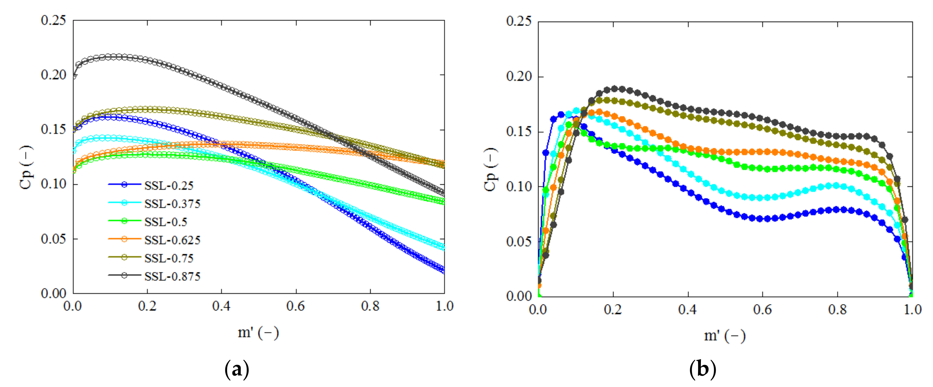
Consequently, the pressure difference at each node can be calculated using the corresponding revised meridional velocity and the circumferential component of absolute velocity, especially when the real blade thickness is taken into account. As a result, the coefficient of pressure difference across the blade is presented in
Figure 9. As expressed by Equation (7), the pressure difference is proportional to the revised meridional velocity and to the derivative of the tangential velocity moment. These two parameters are larger towards the band. Therefore, the pressure difference theoretically increases in the spanwise direction. An overall agreement is observed between the AMOC approach and the Fluent results, though some noticeable discrepancies arise. This may be attributed to the hypotheses, errors during interpolation and the simplifications of this model. In this ambit, the treatment by degenerating the real blade into an S2 surface perhaps had the largest impact, since the AMOC calculates the pressure difference along a spatial streamline, while this value is obtained from the pressure surface and suction surface in the Navier–Stokes solver.
In
Figure 9a, the spanwise
Cp distribution seems to be chaotic due to the shape of the spatially twisted blade, while the streamwise distribution basically declines. During the first half chord, namely 0 < m’ < 0.5, most of the load was applied to the region adjacent to both the crown and the band, whereas the medium region was subjected to less load. On the contrary, the liquid load mainly worked on the downstream region near the band for 0.5 < m’ < 1. This coincides with the higher Eulerian energy near the lower part at the blade outlet, as shown in
Figure 7b and
Figure 8b. It is notable that on the edge of the blade outlet (m′ = 1) the pressure difference is slightly away from zero. This is probably attributed to the enlarged turbulence by the blade-channel vortex and to the outlet residual circulation, which ensured a preferable wake flow and further, a higher runner efficiency. In such a case, the flow pattern leaving the blade fails to meet the Kutta–Joukowski condition. In addition, when
Cp reaches the peak value, the corresponding velocity difference over the blade also becomes the largest. The flow is likely to separate from the blade surface, and this separation can be arithmetically predicted by the definition of stagnation enthalpy in rotational machinery. This scenario will be quantitatively analyzed in the future work combining CFD technology. In summary, the
Cp distribution mainly depends on the blade geometry and flow pattern in the blade channel. By calculating this value, the specific load distribution can be obtained, and the local energy conversion ability on the blade can be clearly evaluated.
4. Conclusions and Outlook
This paper predicted the characteristics of a Francis turbine operated at the BEP by an analytical approach, the AMOC. Implementations of this method were based on differential-geometry theory and the kinematics of ideal fluid, as well as the monistic theory, which was proposed decades ago but is relatively simple and can be efficiently performed. All of these merits make the monistic theory justifiably popular in mathematical models and analytical solutions.
By performing the AMOC procedures, the blade channel was discretized using the spatial relative streamlines, then the relevant hydraulic parameters were calculated, including velocity components, flow angles, Eulerian energy and the pressure difference across the blade. The runner’s optimal hydraulic efficiency was further derived from the Eulerian energy. An arithmetical procedure was proposed to convert the velocity components from the spatial-velocity triangle to the Cartesian coordinate system. The resultant distributions revealed the dynamic evolution of the absolute-velocity vector, magnitude and streamline from the blade inlet to the outlet. Correspondingly, the Eulerian energy was distributed with a similar pattern, and its streamline gradient can represent the energy-conversion ability of the blade. Moreover, the pressure difference derived from flow dynamics elucidates the loading on a blade surface, especially for an X-shaped blade. Herein, most of the loading clusters were near both the crown and the band on the first half of blade, whereas regions near the band dominantly suffered from liquid loading on the downstream half.
The results from the AMOC were compared both to the model test and to the Navier–Stokes solution by the optimal hydraulic efficiency, the absolute velocity, the Eulerian energy and the pressure distribution across the blade. The analytical efficiency value was 94.69%, showing good agreement with the test and numerical simulation. A relevant minor discrepancy and similar flow patterns implied that the proposed AMOC can reliably predict the internal flow field and hydraulic efficiency of a Francis turbine at the BEP. The approach represents a key step towards runner design and selection with short duration and high efficiency.
The basic assumptions of this approach, i.e., inviscid fluid smoothly flowing through the blade channel, hardly deteriorated the precision of predicting the hydraulic efficiency. This satisfactory result is probably attributed to using the length-weighted-average method to calculate the Eulerian energy at the blade inlet and outlet. The uneven energy distribution was therefore cancelled out. Furthermore, the predicted pressure difference at the blade outlet generally coincided with the real conditions despite a slight deviation from the theoretical value. This phenomenon may benefit from a compensation for viscosity and backflow by introducing a blade-blockage factor, or from an induced pressure gradient by the residual circulation at the blade outlet.
One possible improvement to this AMOC approach would be to obtain a better prediction of the pressure difference, especially in the region near the blade inlet. In the AMOC approach, the blade degenerated to a smooth stream surface. However, the blade shape near the leading edge had a large curvature due to better dynamic characteristics. Therefore, it is in fact possible to carefully deal with the region adjacent to the blade’s leading edge.
5. Patents
Yu Chen, Jianxu Zhou, Wenqing Jiang, et al. Calculation methodology and system of the best efficiency for a hydraulic reaction runner: China, ZL201810870576.1[P]. 21 April 2020.
Author Contributions
Conceptualization, methodology, computation, visualization, writing-original draft, Y.C.; methodology, resources, supervision, writing-review and editing, J.Z. (Jianxu Zhou) and B.K.; formal analysis, validation, writing-review, Q.G.; funding acquisition, J.Z. (Jianxu Zhou) and J.Z. (Jian Zhang). All authors have read and agreed to the published version of the manuscript.
Funding
This research was funded by the National Natural Science Foundation of China, grant number 51879087, 51839008, by the High-education Natural Science Foundation of Jiangsu Province, grant number 21KJB570001, and by the Research Foundation for High-level Talents of NJIT, grant number YKJ202131.
Institutional Review Board Statement
Not Applicable.
Informed Consent Statement
Not Applicable.
Data Availability Statement
Not Applicable.
Acknowledgments
The authors would like to thank the support by the China Scholarship Council and the Harbin electrical machine factory in China.
Conflicts of Interest
The authors declare no conflict of interest.
Appendix A
Appendix A.1. Coordinate Transformation
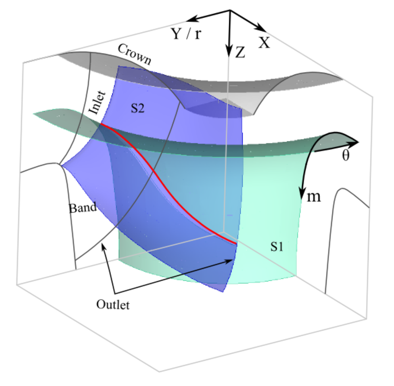
Two definitions are introduced firstly, the stream surface (S1) and the blade chamber surface (S2). S1 is a rotational symmetric surface such as the trumpet-shaped light-green face in
Figure A1. It defines the flow trajectory in the channel without a blade from the radial to the axial direction. S2 is identical to the real blade surface when the runner has an infinite number of infinitely thin blades, such as the purple face in
Figure A1. Meanwhile, S2 can be composed of the chamber lines of the spanwise blade cascade. Therefore, S2 is named the blade-chamber surface. In
Figure A1, a curved coordinate system (
m,
θ) located on the S1 surface is established. The θ–axis denotes the azimuthal direction on the horizontal plane, while the m-axis denotes the generatrix line of the S1 surface on the vertical plane. The spatial relative streamline (SSL), which is the intersection of S1 and S2, is marked as the red curve in
Figure A1. Node coordinates on this streamline are therefore converted from a Cartesian system to the (
m,
θ) system, expressed as:
where
i denotes the
ith node on the SSL. (
xi,
yi,
zi) denotes the coordinates of the
ith node in the Cartesian system. (
mi,
θi) denotes the coordinates of the
ith node in the curved system. (
x0,
y0) are the coordinates of the SSL origin. Δ
zi =
zi −
zi−1 is the axial interval of the adjacent nodes. Δ
ri =
ri −
ri−1 is the radial interval of the adjacent nodes.
Figure A1.
Blade-chamber surface, stream surface and their meridian projection.
Figure A1.
Blade-chamber surface, stream surface and their meridian projection.
Figure A2.
Generatrix of flow cross section in blade channel.
Figure A2.
Generatrix of flow cross section in blade channel.
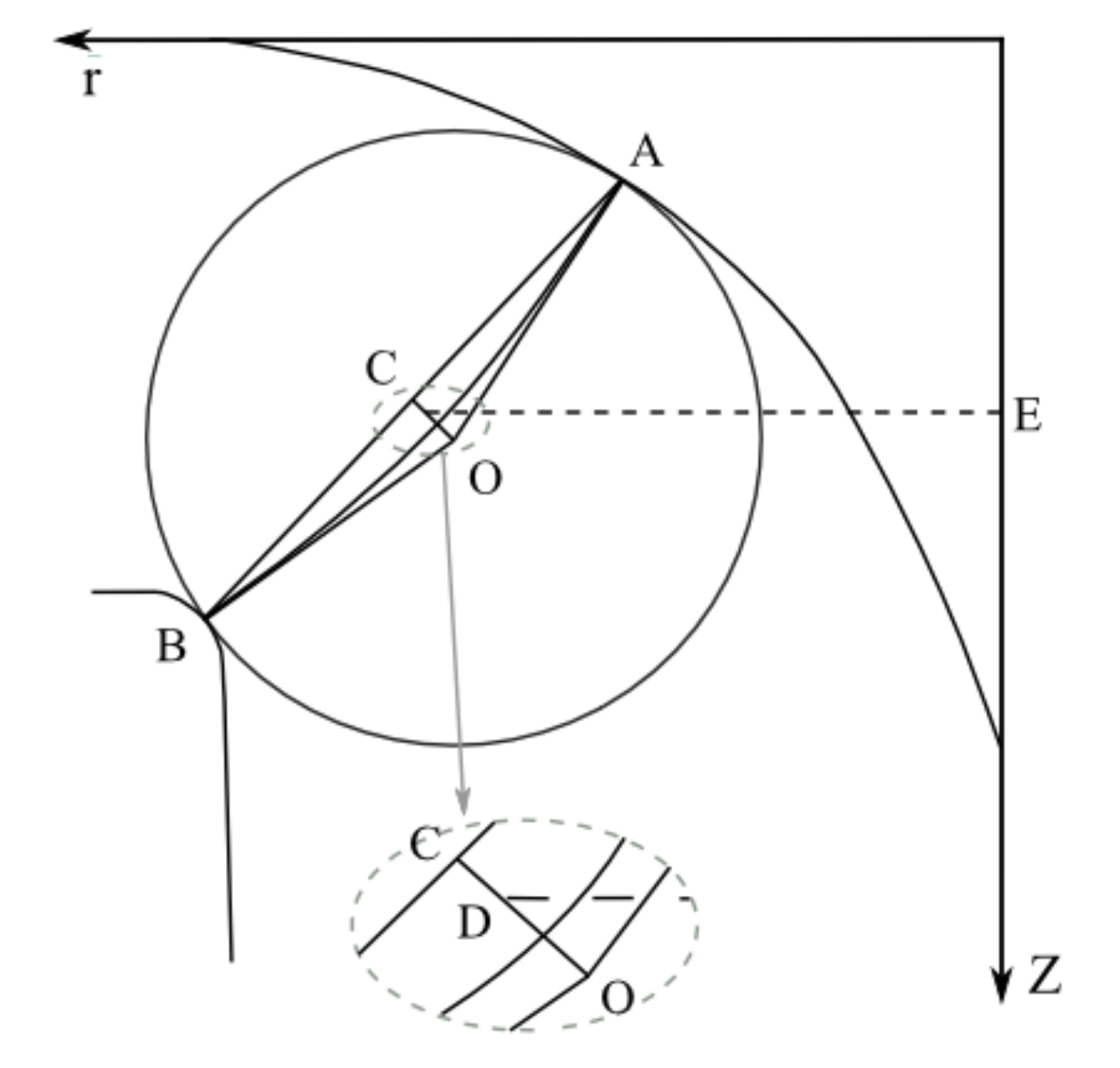
Appendix A.2. Generatrix of Flow Section and Meridional Velocity
In the meridional plane in
Figure A2, an inscribed circle tangents to both the crown and the band with tangency points A and B. OA and OB denote the radius of the circle with the center O. Then, the generatrix can be equivalent to the arc
, which is tangent to the radius OA and OB, respectively, on points A and B. Its length can be calculated by the following empirical formula:
where
is the radius value and
is the chord length.
Then, the arc
rotates around the
Z-axis to obtain the flow cross section. Its area
S and meridian velocity
Vm are subsequently computed:
where line OC is perpendicular to the chord AB. Point D is located on 1/3 of the line OC, and the length
.
Q0 denotes the discharge at the BEP.
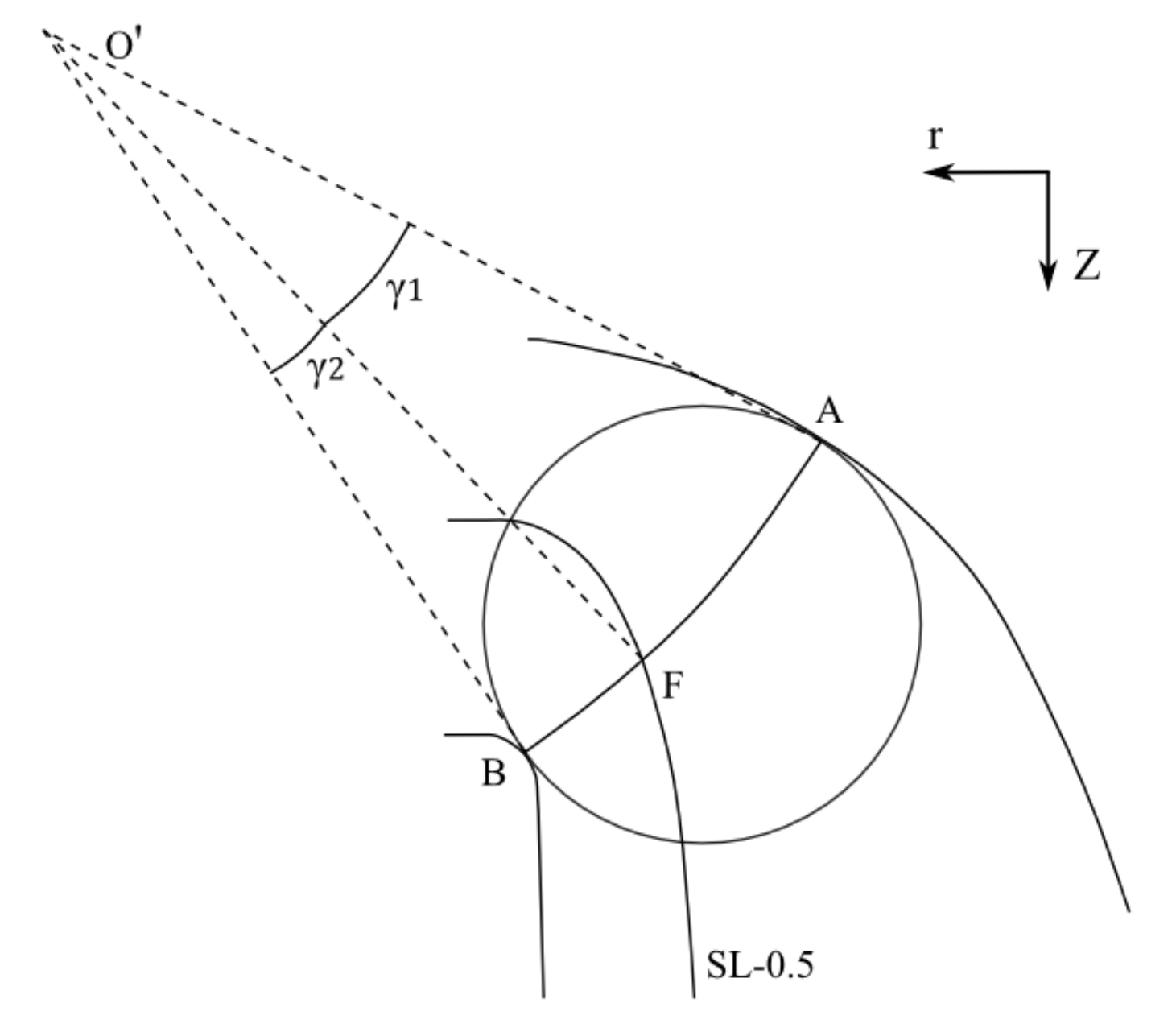
Appendix A.3. Streamline Cluster Generation
The meridional channel is discretized by the meridional streamlines. An example of the medium streamline, named SL-0.5, is presented in
Figure A3. It divides the channel into two parts. The coordinates of point F, which are the intersection of generatrix
and SL-0.5, can be derived by the following equations. Equations (A8)–(A10) are established by geometrical features and Formula (A11) defines the same discharge passing arc
and arc
.
where (
r,
z) with different subscripts denotes the coordinates of corresponding points.
is the center of arc
.
R denotes its radius.
and
denote the radian angle of
and
.
With various inscribed circles in the meridional channel, a series of intersection points are obtained, which then make up the streamline SL-0.5. In the same manner, SL-0.25 is produced, thereby evenly dividing the region between SL-0.5 and the crown. Likewise, SL-0.75 halves the channel between SL-0.5 and the band.
Subsequently, the S1 stream surface is established by rotating the meridional streamline around the
Z-axis. Meanwhile, the S2 surface is defined by the centers of incircles and their tangency points in the wooden blade figures. The resultant relative spatial streamline is then generated by intersecting the S1 and S2 surfaces, named SSL-No., where the No. coincides with the number of the SL. Finally, ten SSLs including the crown and the band are illustrated in
Figure A4. They represent ideal flow trajectories on the blade surface. Additionally, the origins and endpoints of these lines are separately located on the blade’s leading edge and trailing edge.
Figure A3.
Sketch of meridional streamline.
Figure A3.
Sketch of meridional streamline.
Figure A4.
Sketch of spatial relative streamline.
Figure A4.
Sketch of spatial relative streamline.
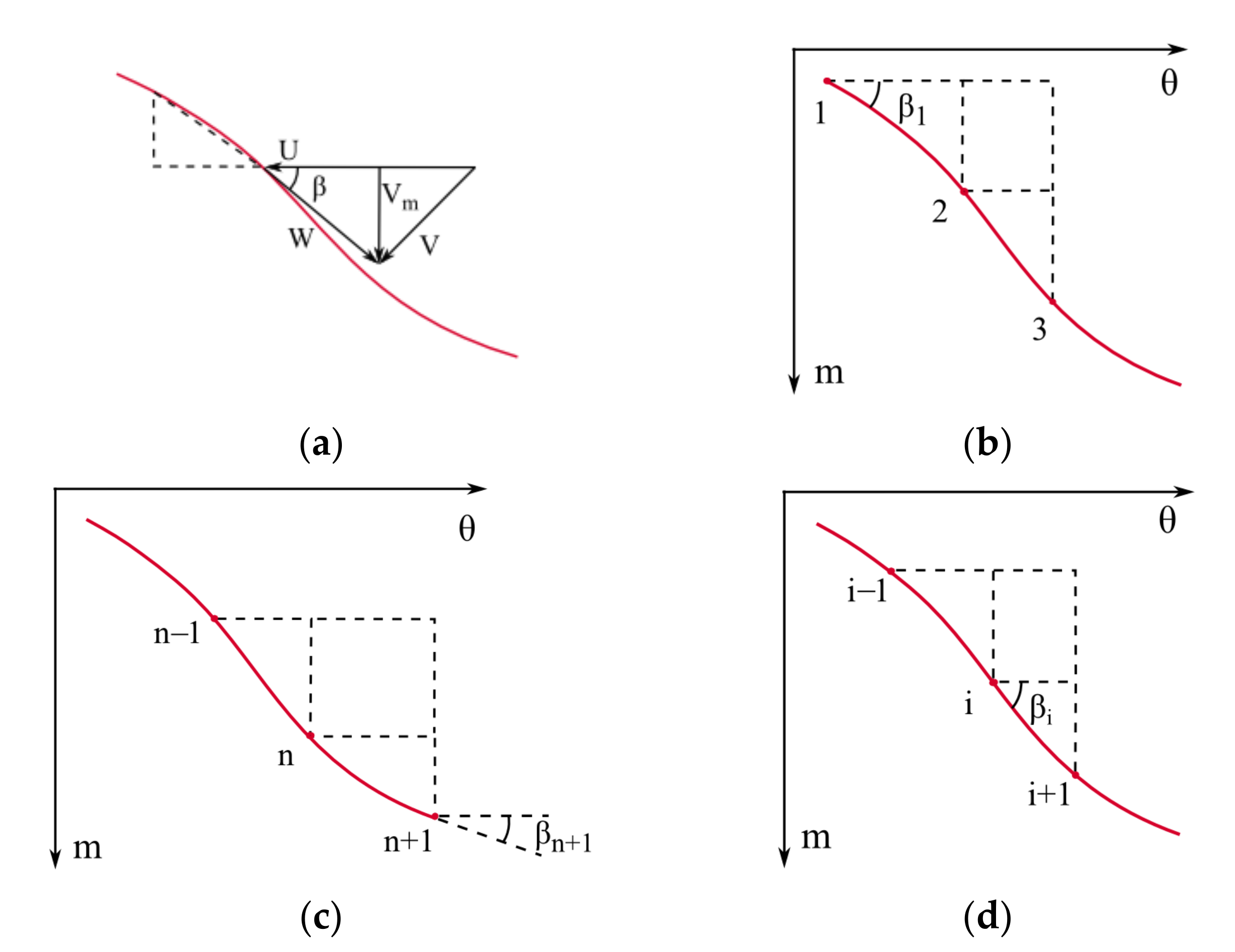
Appendix A.4. Relative Flow Angle
Figure A5 shows the projection of the (
m,
θ) coordinates, velocity triangle and spatial streamline onto a plane. The spatial streamline is evenly divided into
n segments in order to further discretize the spatial flow field. According to the third assumption, the relative flow angle (
β) in
Figure A5a at each node can be derived from interpolating the angles between the local tangent and the horizontal direction. Considering different positions of the node, three scenarios are presented as follows, and the corresponding schematic of the flow angle is shown in
Figure A5b–d, respectively.
where
βi denotes the relative flow angle at the
ith node and
τi denotes the interpolating coefficient.
Figure A5.
Velocity triangle and flow angle at different locations on SSL: (a) velocity triangle; (b) origin of streamline; (c) endpoint of streamline; (d) medium positions.
Figure A5.
Velocity triangle and flow angle at different locations on SSL: (a) velocity triangle; (b) origin of streamline; (c) endpoint of streamline; (d) medium positions.
Appendix A.5. Meridional Velocity at SSL Nodes and Effects of Blade Thickness
It is notable that the SL is the meridional projection of the corresponding SSL, so they have identical m-axial components. Additionally, Equation (A7) defines the distribution of Vm on SL. Therefore, based on the (m, Vm) pairs on the SL, Vm at each node on the SSL is subsequently interpolated.
In addition, blade thickness, to some extent, blocks the flow passage, changing the velocity’s magnitude and direction. Herein, the AMOC is only concerned with its effect on magnitude, while the flow direction is kept aligned with the SSL and the blocked flow passage is subjected to the unchanged discharge, which is expressed by:
where
ri denotes the radius of the
ith node.
N denotes the blade number.
ei denotes the corresponding thickness derived from diameter of the incircles in the wooden blade figure.
Vm′ denotes the revised meridional velocity at node
i. Then the blockage factor, accounting for the thickness effect, is defined as:
Appendix A.6. Velocity Triangle
According to the resolved parameters, each component in the velocity triangle at every node can be computed. By extension, in the triangle sketched in
Figure A5a, the circumferential velocity component is:
where
ω is the angular speed and
n0 is the rated rotation speed.
By recalling the Law of sines, the relative velocity is:
With the Law of cosines in the velocity triangle, the velocity components and flow angles satisfy the following equations:
Thus, the absolute velocity
Vi and the corresponding absolute flow angle
αi can be calculated. Then,
Vi is projected in the circumferential direction as:
where
VUi denotes the tangential component of
Vi at node
i.
References
- Zhang, Y.; Zheng, X.; Li, J.; Du, X. Experimental study on the vibrational performance and its physical origins of a prototype reversible pump turbine in the pumped hydro energy storage power station. Renew. Energy 2019, 130, 667–676. [Google Scholar] [CrossRef]
- Trivedi, C.; Gogstad, P.J.; Dahlhaug, O.G. Investigation of the unsteady pressure pulsations in the prototype Francis turbines—Part 1: Steady state operating conditions. Mech. Syst. Sig. Process. 2018, 108, 188–202. [Google Scholar] [CrossRef] [Green Version]
- Zhang, L.; Wu, Q.; Ma, Z.; Wang, X. Transient vibration analysis of unit-plant structure for hydropower station in sudden load increasing process. Mech. Syst. Sig. Process. 2019, 120, 486–504. [Google Scholar] [CrossRef]
- Li, D.; Sun, Y.; Zuo, Z.; Liu, S.; Wang, H.; Li, Z. Analysis of Pressure Fluctuations in a Prototype Pump-Turbine with Different Numbers of Runner Blades in Turbine Mode. Energies 2018, 11, 1474. [Google Scholar] [CrossRef] [Green Version]
- Gohil, P.P.; Saini, R.P. Numerical Study of Cavitation in Francis Turbine of a Small Hydro Power Plant. J. Appl. Fluid Mech. 2016, 9, 357–365. [Google Scholar] [CrossRef]
- Decaix, J.; Müller, A.; Favrel, A.; Avellan, F.; Münch, C. URANS Models for the Simulation of Full Load Pressure Surge in Francis Turbines Validated by Particle Image Velocimetry. J. Fluids Eng. 2017, 139, 121103. [Google Scholar] [CrossRef]
- Favrel, A.; Müller, A.; Landry, C.; Yamamoto, K.; Avellan, F. Study of the vortex-induced pressure excitation source in a Francis turbine draft tube by particle image velocimetry. Exp. Fluids 2015, 56, 215. [Google Scholar] [CrossRef]
- Skripkin, S.; Tsoy, M.; Kuibin, P.; Shtork, S. Swirling flow in a hydraulic turbine discharge cone at different speeds and discharge conditions. Exp. Therm. Fluid Sci. 2019, 100, 349–359. [Google Scholar] [CrossRef]
- Lai, X.; Liang, Q.; Ye, D.; Chen, X.; Xia, M. Experimental investigation of flows inside draft tube of a high-head pump-turbine. Renew. Energy 2019, 133, 731–742. [Google Scholar] [CrossRef]
- Leguizamón, S.; Avellan, F. Open-Source Implementation and Validation of a 3D Inverse Design Method for Francis Turbine Runners. Energies 2020, 13, 2020. [Google Scholar] [CrossRef] [Green Version]
- Li, W. Inverse design of impeller blade of centrifugal pump with a singularity method. Jordan J. Mech. Ind. Eng. 2011, 5, 119–128. [Google Scholar]
- Zangeneh, M.; Goto, A.; Takemura, T. Suppression of secondary flows in a mixed-flow pump impeller by application of 3D inverse design method. In International Gas Turbine and Aeroengine Congress and Exposition; ASME: Hague, The Netherlands, 1994. [Google Scholar]
- Hawthorne, W.R.; Wang, C.; Tan, C.S.; Mccune, J.E. Theory of Blade Design for Large Deflections: Part I—Two-Dimensional Cascade. J. Eng. Gas Turbines Power 1984, 106, 346–353. [Google Scholar] [CrossRef]
- Yin, J.; Wang, D. Review on applications of 3D inverse design method for pump. Chin. J. Mech. Eng. 2014, 27, 520–527. [Google Scholar] [CrossRef]
- Kan, K.; Chen, H.; Zheng, Y.; Zhou, D.; Binama, M.; Dai, J. Transient characteristics during power-off process in a shaft extension tubular pump by using a suitable numerical model. Renew. Energy 2021, 164, 109–121. [Google Scholar] [CrossRef]
- Kan, K.; Yang, Z.; Lyu, P.; Zheng, Y.; Shen, L. Numerical Study of Turbulent Flow past a Rotating Axial-Flow Pump Based on a Level-set Immersed Boundary Method. Renew. Energy 2021, 168, 960–971. [Google Scholar] [CrossRef]
- Qian, H.; Chen, N.; Lin, R.; Qu, L.; Pu, S. Design of mixed flow pump impeller by using direct-inverse problem iteration. J. Hydraul. Eng. 1997, 1, 25–30. [Google Scholar]
- Bing, H.; Zhang, Q.; Cao, S.; Tan, L.; Zhu, B. Iteration design of direct and inverse problems and flow analysis of mixed-flow pump impellers. J. Tsinghua Univ. 2013, 53, 179–183. [Google Scholar]
- Tan, L.; Cao, S.; Wang, Y.; Zhu, B. Direct and inverse iterative design method for centrifugal pump impellers. J. Power Energy 2012, 226, 764–775. [Google Scholar] [CrossRef]
- Bing, H.; Cao, S.; Tan, L. Iteration method of direct inverse problem of mixed-flow pump impeller design. J. Drain. Irrig. Mach. Eng. 2011, 29, 277–281. [Google Scholar]
- Ciocan, T.; Susan-Resiga, R.F.; Muntean, S. Modelling and optimization of the velocity profiles at the draft tube inlet of a Francis turbine within an operating range. J. Hydraul. Res. 2016, 54, 74–89. [Google Scholar] [CrossRef]
- Chen, Z.; Singh, P.M.; Choi, Y.-D. Francis Turbine Blade Design on the Basis of Port Area and Loss Analysis. Energies 2016, 9, 164. [Google Scholar] [CrossRef] [Green Version]
- Yin, J.; Li, J.; Wang, D.; Wei, X. A simple inverse design method for pump turbine. IOP Conf. Ser. Earth Environ. Sci. 2014, 22, 012030. [Google Scholar] [CrossRef]
- Han, F.; Huang, L.; Yang, L.; Kubota, T. Geometrical analysis of adjustable guide vanes for bulb turbine. J. Eng. Thermophys. 2010, 31, 263–266. [Google Scholar]
- Liu, P. Channel Theory for High-Head Bulb Runner; South China University of Technology: Guangzhou, China, 2010. [Google Scholar]
- Susan-Resiga, R.F.; Milos, T.; Baya, A.; Muntean, S.; Bernad, S. Mathematical and Numerical Models for Axisymmetric Swirling Flows for Turbomachinery Applications. Sci. Bull. Univ. Politeh. Timis. Trans. Mech. 2005, 50, 47–58. [Google Scholar]
- Susan-Resiga, R.; Ighişan, C.; Muntean, S. A Mathematical Model for the Swirling Flow Ingested by the Draft Tube of Francis Turbines. WasserWirtschaft 2015, 13, 23–27. [Google Scholar] [CrossRef]
- Susan-Resiga, R.F.; Muntean, S.; Avellan, F.; Anton, I. Mathematical modelling of swirling flow in hydraulic turbines for the full operating range. Appl. Math. Modell. 2011, 35, 4759–4773. [Google Scholar] [CrossRef]
- Susan-Resiga, R.F.; Avellan, F.; Ciocan, G.D.; Muntean, S.; Anton, I. Mathematical and Numerical Modelling of the Swirling Flow in Francis Turbine Draft Tube Cone. Sci. Bull. Univ. Politeh. Timis. Trans. Mech. 2005, 50, 1–16. [Google Scholar]
- Muntean, S.; Susan-Resiga, R.; Göde, E.; Baya, A.; Terzi, R.; Tîrşi, C. Scenarios for refurbishment of a hydropower plant equipped with Francis turbines. Renew. Energy Environ. Sustain. 2016, 1, 30. [Google Scholar] [CrossRef]
- Brekke, H. Hydraulic Turbines. Design, Erection and Operation; Norwegian University of Science and Technology: Trondheim, Norway, 2001. [Google Scholar]
- Brekke, H. Performance and safety of hydraulic turbines. In 25th IAHR Symposium on Hydraulic Machinery and Systems; IOP Publishing: Bristol, UK, 2010. [Google Scholar]
- Leguizamón, S.; Ségoufin, C.; Phan, H.T.; Avellan, F. On the efficiency alteration mechanisms due to cavitation in Kaplan turbines. J. Fluids Eng. 2017, 139, 061301. [Google Scholar] [CrossRef]
- Li, W.; Gong, R. The Researching of Turbine Main Parameters Selection for Three Gorges Right Bank Power Station. Large Electr. Mach. Hydraul. Turbine 2009, 2, 37–42. [Google Scholar]
- Wang, G. Key Technologies for Huge Full Air-cooled Hydrogenerator Sets of Three Gorges Right Bank Power Station—Hydraulic Turbine Section. Large Electr. Mach. Hydraul. Turbine 2008, 4, 30–36. [Google Scholar]
- Daneshkah, K.; Zangeneh, M. Parametric design of a Francis turbine runner by means of a three-dimensional inverse design method. IOP Conf. Earth Environ. Sci. 2010, 12, 012058. [Google Scholar] [CrossRef]
| Publisher’s Note: MDPI stays neutral with regard to jurisdictional claims in published maps and institutional affiliations. |
© 2022 by the authors. Licensee MDPI, Basel, Switzerland. This article is an open access article distributed under the terms and conditions of the Creative Commons Attribution (CC BY) license (https://creativecommons.org/licenses/by/4.0/).


