Investigation into Influence of Wall Roughness on the Hydraulic Characteristics of an Axial Flow Pump as Turbine

Abstract

Pump as turbine (PAT) is a factual alternative for electricity generation in rural and remote areas where insufficient or inconsistent water flows pose a threat to local energy demand satisfaction. Recent studies on PAT hydrodynamics have shown that its continuous operations lead to a progressive deterioration of inner surface smoothness, serving the source of near-wall turbulence build-up, which itself depends on the level of roughness. The associated boundary layer flow incites significant friction losses that eventually deteriorate the performance. In order to study the influence of wall roughness on PAT hydraulic performance under different working conditions, CFD simulation of the water flow through an axial-flow PAT has been performed with a RNG k-ε turbulence model. Study results have shown that wall roughness gradually decreases PAT’s head, efficiency, and shaft power. Nevertheless, the least wall roughness effect on PAT hydraulic performance was experienced under best efficiency point conditions. Wall roughness increase resulted in the decrease of axial velocity distribution uniformity and the increase of velocity-weighted average swirl angle. This led to a disorderly distribution of streamlines and backflow zones formation at the conduit outlet. Furthermore, the wall roughness impact on energy losses is due to the static pressure drop on the blade pressure surface and the increase of turbulent kinetic energy near the blade. Further studies on the roughness influence over wider range of PAT operating conditions are recommended, as they will lead to quicker equipment refurbishment.

1. Introduction

Under low-head operating conditions, axial flow pumps are more likely to exhibit good hydraulic performance characteristics. Hence, these pumps are suitable for large- and medium-sized pumping stations in plain areas, where they play a vital role in urban water supply and agricultural irrigation [1,2]. According to the installation position of the pump shaft, axial flow pumps can be classified into three types: vertical, horizontal, and slanted pumps. Conversely to the vertical type, slanted axial flow pump’s inlet conduit does not need 90° elbow, which relatively explains its low hydraulic loss. Compared with the horizontal type, the slanted axial flow pump has better performance, since the connected electric motor does not have to be installed underwater [3,4]. Axial flow pump has been widely applied in the eastern route of China’s South-to-North Water Diversion Project. Due to the landform and climate reasons, wet seasons are dominated by a lot of floods and stagnant waters. To achieve considerable economic benefits, pumping stations can make full use of such water energy resources by means of pump as turbine (PAT) technology [5,6]. Thanks to the control valve utilization, the flow direction can be reversed for power generation. The pump technology has grown mature to reach a convenient maintenance routine and a fair affordability [7]. Many recent projects have endeavored to replace conventional small hydropower units with pumps in order to meet the energy demand in remote regions. However, the efficiency of PATs is still relatively low [8]. In addition, due to the influence of manufacturing processes, the inner wall surface cannot be perfectly smooth; i.e., the wall roughness of the machine is not uniform. After a certain operation period, PAT performance ends up deteriorating as sedimentation, oxidation, and corrosion accumulate over time. Such accumulation jointly increases the surface irregularities of the conveying structure and leads to declining hydraulic performance [9]. With the improvement of water supply projects and drainage irrigation, the safety and stable operation of axial flow pumps have been a research priority [10]. Therefore, the study of the influence of wall roughness on hydraulic performance of the axial flow PAT can be very useful for the daily maintenance of pump stations.

Lin et al. [11] used numerical methods to predict PAT performance curves under both the pump and turbine operating modes, and verified them experimentally. Yang et al. [12] used CFD to simulate the influence of splitter blades on PATs. The addition of splitter blades came up with a great performance improvement in operation efficiency. Comparison between experimental and numerical results showed that CFD can be used in the performance prediction and optimization of PAT. A novel impeller design has been proposed to retrofit conventional double suction pump. With the open source CFD code OpenFOAM, the novel impeller has been investigated in turbine mode using 3D URANS simulations and the characteristic curves of the two machines have been calculated and compared [13]. Derakhshan et al. [14] redesigned the shape of impeller blades leading its efficiency improvement as compared to experimental data. It was noted that PAT efficiency can be improved just by impeller modification. On the other hand, PAT volute casing’s cutwater design can also influence its performance characteristics, as noted by Morabito et al. [15].

As shown in the above literature, CFD has been an important tool in studies on PAT flow dynamics. In the same respect, it has crucially contributed to the attainment of an in-depth understanding about wall roughness effect and the underlying flow instability development mechanism. Gu et al. [16] found that the influence of surface roughness on pump hydraulic performance depends on the actual roughness of the structure, velocity distribution, and near-wall turbulence along the flow path. A study by Bai Tao et al. [17] revealed a close relationship between the surface roughness in the boundary layer and the operational Reynolds number, for a wind turbine case. At low Reynolds numbers, surface roughness could weaken separation bubbles, lowering the aerodynamic losses. On the other hand, operations at high Reynolds numbers suffered significant losses due to transient processes triggered by surface roughness. For the case of hydraulic pumps, Bellary et al. [18] found that wall roughness increases with the head and shaft power, while hydraulic efficiency correspondingly decreased. In the same respect, Deshmukh et al. [19] studied the influence of wall roughness on centrifugal pumps hydraulic performance under optimal and off-design conditions. For completely rough surfaces, the hydraulic performance of centrifugal pumps has displayed a progressive deterioration. When the roughness critical value was reached, the hydraulic performance stopped declining, where further decrease yielded slight head increase. Within the same context, Juckelandt et al. [20] comparatively analyzed the influence of surface roughness on the pump performance by means of experiments and simulations. The influence of roughness on flow parameters such as the average velocity and turbulence pulsations was investigated. He et al. [21] conducted a series of numerical calculations of different turbulence models and surface roughness for a multistage centrifugal pump based on CFD. The results came up with the same conclusion that the surface roughness strongly affects the head and efficiency. However, the impact gradually slows down, and the effect of surface roughness on efficiency is greater than that of head. Limbach et al. [22] carried out experimental measurements and numerical simulation on cavitation flow within a low specific speed centrifugal pump under different working conditions and different roughness surface. The results showed that, in the flow without cavitation, the head measured and simulated adamantly stays consistent, and the experimental measurements drew an inference that with the worsening of surface roughness, the net positive suction head (NPSH) increases significantly. Nonetheless, this finding has not been reproduced by simulations of the wall function.

To cut short this overview of the literature relevant to the present study, Lim et al. [23] have carried out the study on the similar investigation on a dual-suction centrifugal pump. They came up with a conclusion that the roughness has the greatest influence on the impeller, while the inlet conduit flow does not reflect that high ascendancy. In addition, the pump performance has been found to largely depend on the surface roughness on the impeller shroud. So far, the existent literature about the influence of wall roughness on hydraulic machinery performance is predominantly focused on centrifugal pumps, where comparatively few studies have been conducted on axial-flow pumps, and the generating mode of PATs is rarely investigated. Moreover, most of studies have investigated the effect of surface roughness on the machine’s external performance characteristics (EPCs), using experimental and numerical simulation methods without digging deeper to the root cause of recorded changes in machine EPCs. Therefore, the influence of surface roughness on PAT’s internal flow dynamics is still inadequately studied.

In this respect, the present article evaluates the hydraulic performance of a slanted axial flow PAT subjected to different wall roughness scenarios. The influence of wall roughness on the internal flow state of an axial flow PAT under different flow conditions for a wide range of roughnesses is analyzed in order to improve the equipment integrity rate and operational life span. This study’s results provide a useful reference for pump station optimization. The article structure comprises four sections organized as follows: Section 2 details the applied methodology concept, where the concerned PAT’s geometric model, as well as the utilized numerical method, are well presented. For an analogic understanding of the subject matter, the theory of equivalent sand-grain roughness is briefly recapitulated, as well. The results of this study, including the external performance characteristics of the slanted axial flow PAT and the influence of wall roughness on the same, are presented and discussed within Section 3. Finally, to draw this work to a close, relevant conclusions and further research recommendations have been pointed out through Section 4.

2. Numerical Model and Methods

2.1. Governing Equations

The continuity and momentum equations that are extensively used in flow diagnostics are stated through Equations (1) and (2) [24,25]:

$$\frac{\partial \rho }{\partial t}+\frac{\partial (\rho u_i)}{\partial x_i}=0$$

(1)

$$\frac{\partial (\rho u_i)}{\partial t}+\frac{\partial (\rho u_i{u}_j)}{\partial x_j}=-\frac{\partial p}{\partial x_i}+\frac{\partial }{\partial x_j}(\mu \frac{\partial u_i}{\partial x_j})+\frac{\partial {\tau }_{ij}}{\partial x_j}$$

(2)

where the following designation applies ρ: the density, t: the physical time, p: the local pressure, μ: the dynamic viscosity, τ_ij: the Reynolds stress; whereas x_i and x_j represent the Cartesian coordinate components in the i and j directions, respectively, u_i and u_j represent the corresponding components of the time-averaged velocity.

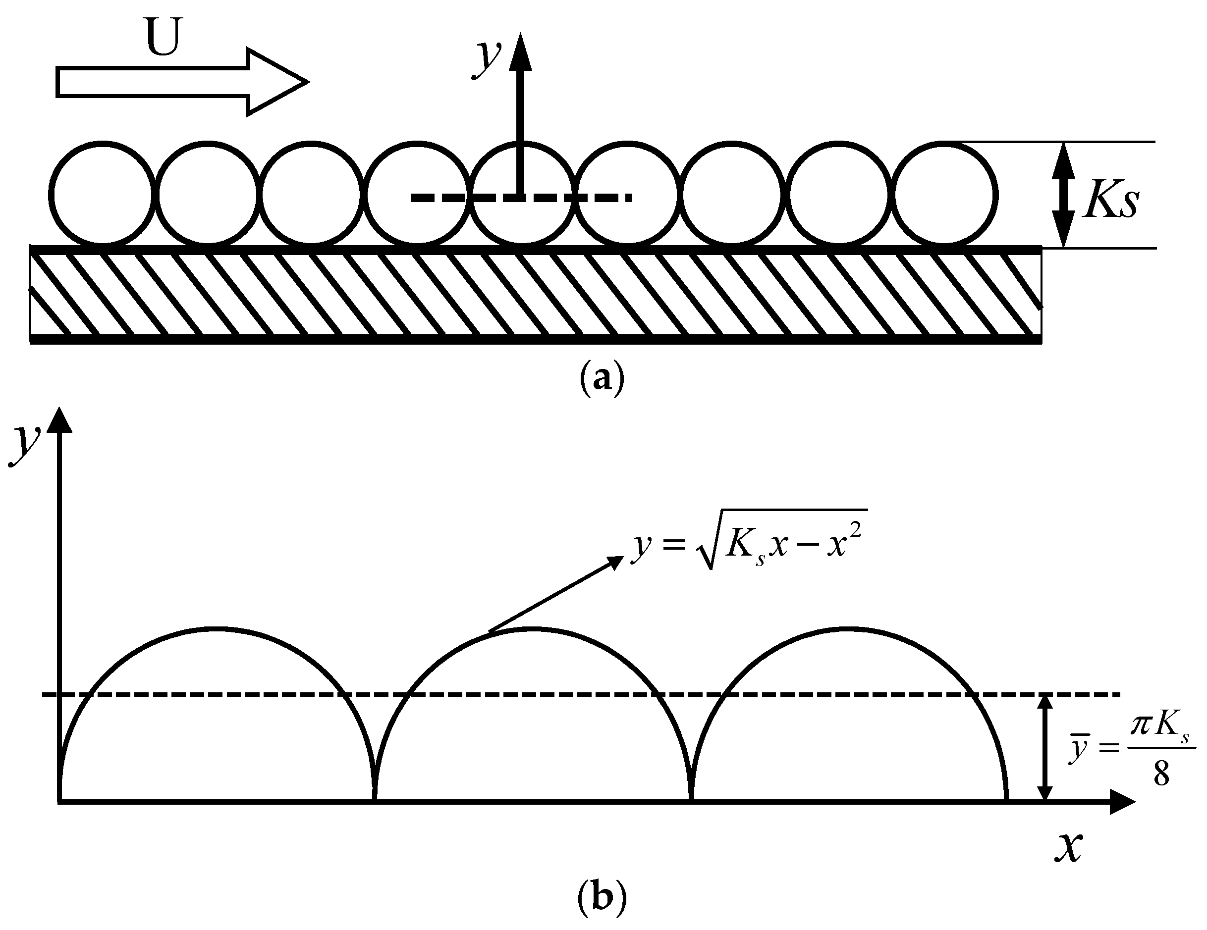
2.2. Equivalent Sand-Grain Roughness

The wall roughness is indicated through the consideration of peaks and valleys under different shapes and sizes. It is convenient to simulate that surface texture with an equivalent analogy of sand-grain roughness. Figure 1a depicts that similarity by using a wall with a layer of closely packed spheres [26]. The average roughness height of the spheres is K_s [μm], also known as equivalent sand height [27]. The friction effect only occurs in the upper part of balls, and the equivalent sand-grain roughness only affects the flow in its vicinity. Therefore, the actual flow surface may be rounded as shown in Figure 1b, where the x-axis represents the physical wall surface.

Roughness is the measure of the micro spacing and peak-valley unevenness on the surface texture. The arithmetic average of absolute value (R_a) that is used to quantify the surface roughness is couched in Equation (3).

$$R_a=\frac{1}{n}{\displaystyle \sum _{i=1}^n\left|y_i\right|}$$

(3)

where y_i is the distance from the average height of a profile (the mean line) for measurement i, and n is the number of measurements [28]. As the number of measurements approaches infinity, Equation (3) tends to look like Equation (4).

$$R_a=\frac{1}{K_s}{\displaystyle {\int }_{x=0}^{K_s}\left|y-\overline{y}\right|}dx$$

(4)

Considering parameters in Equation (4), the equation of wall roughness profile can be formulated as to Equation (5) and the mean line as to Equation (6).

$$y=\sqrt{K_{s}x-x^2}$$

(5)

$$\overline{y}=\frac{\pi K_s}{8}$$

(6)

Substitute Equations (7) and (8) into Equation (6) and integrate:

$$R_a=\frac{K_s}{2}\left(\frac{\pi }{2}-{\cos }^{-1}{\left(1-\frac{{\pi }^2}{16}\right)}^{1/2}-\frac{\pi }{4}{\left(1-\frac{{\pi }^2}{16}\right)}^{1/2}\right)$$

(7)

Simplify the Equation (7), the average roughness height of the spheres (K_s) can be expressed as to Equation (8).

$$K_{\mathrm{s}}=11.0293R_a$$

(8)

2.3. The Geometric Model Description

The wall roughness involves the entire hydraulic circuit of a slanted axial flow pump. Therefore, the computational domain consists of four main parts of inlet conduit, impeller, guide vane and outlet conduit, as shown in Figure 2. Design and operation parameters of the investigated hydraulic machine are specified in

Table 1. Parameters of the slanted axial flow pump.

Parameter	Value
Impeller nominal diameter D [m]	3.25
Design head H [m]	2.6
Design flow rate Q [m3/s]	45.5
Design power P [kW]	1319
Design efficiency η [%]	88
Rotational speed n [r/min]	122

.

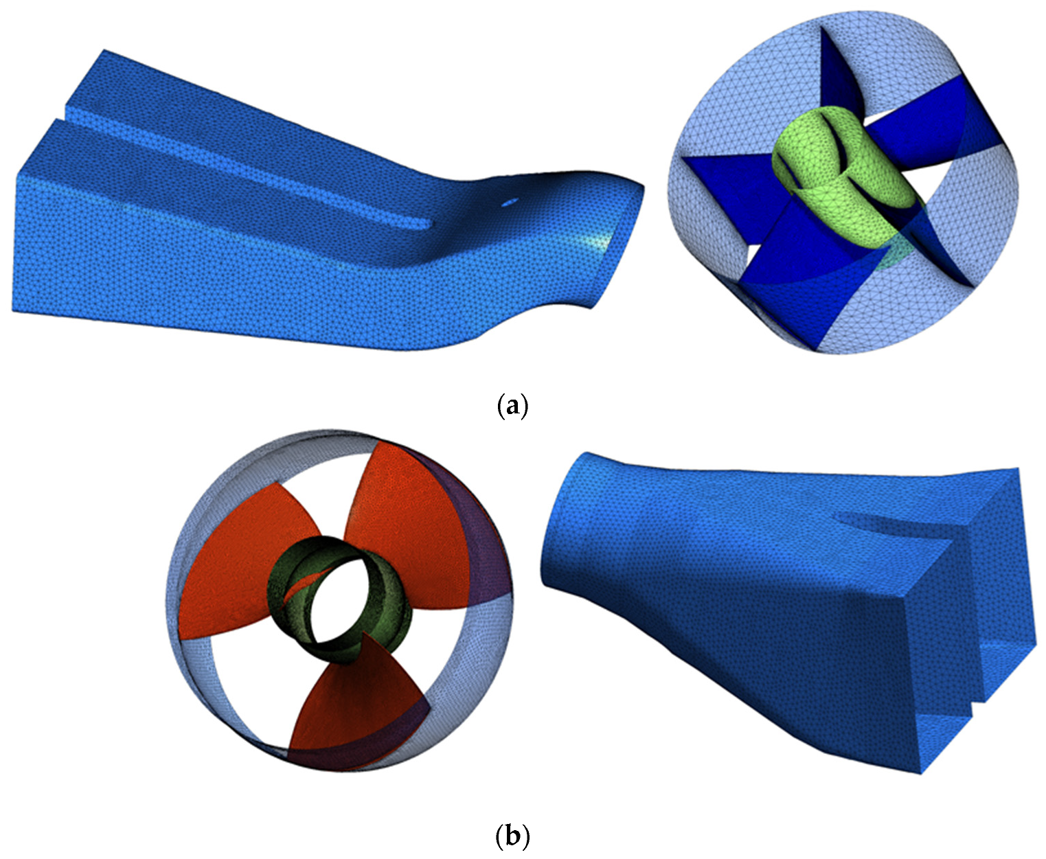
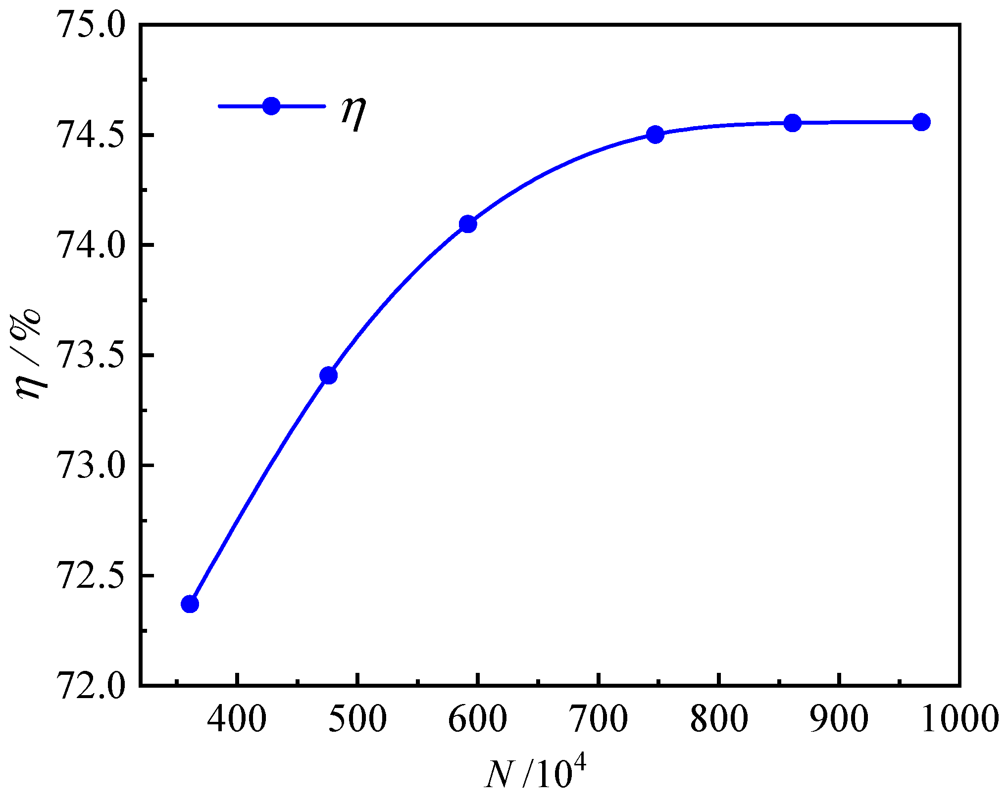
2.4. The Grid Generation Methodology

To generate the mesh of PAT’s computational domain, the unstructured type of computational grid (Figure 3) has been adopted to deeply resolve the hectic flow dynamicity in the rough wall’s vicinal flow zones. To capture the effect of roughness on near-wall flow more precisely, local grid refinement was carried out, and wall function method was adopted within that critical zone of activity. In order to determine the appropriate grid number for further simulations; a grid independence test has been conducted. To do this, six grid size sets have been generated and simulated under similar boundary conditions, leading to six different PAT performances in terms of a single common parameter, namely the PAT hydraulic efficiency (η). The curve in Figure 4 is the delineation of how PAT hydraulic efficiency varies with the change in grid number under pump-mode operation for the similar flow rate.

From Figure 4, it is obvious that when the grid number reaches 7.48 million, the efficiency tends to display a relatively stable pattern. To that end, the grid size of 7.48 million has been selected for further numerical simulations, as it features the desired advantages of calculation accuracy and the computation cost in terms of simulation time [29]. The grid number in each part of the computational model is shown in

Table 2. Grid repartition per each component.

Hydraulic Circuit Components	Grid Size [104]
Inlet conduit	79
Guide vane	241
Impeller	334
Outlet conduit	94
An all-embracing grid size	748

.

2.5. Boundary Conditions

ANSYS Fluent is applied to simulate the steady incompressible flow of the slanted axial-flow PAT. The finite volume method is used for space discretization, and the pressure velocity coupling is realized by SIMPLEC algorithm. The inlet boundary condition of the computational domain has been set to be the mass flow inlet, and the outlet boundary condition was set as pressure outlet. The impeller domain was based on the rotating reference frame, while the other domains were based on the stationary reference frame. All wall boundaries adopted non-slip walls, and the convergence criterion is set to 1 × 10⁻⁵.

3. Results and Discussion

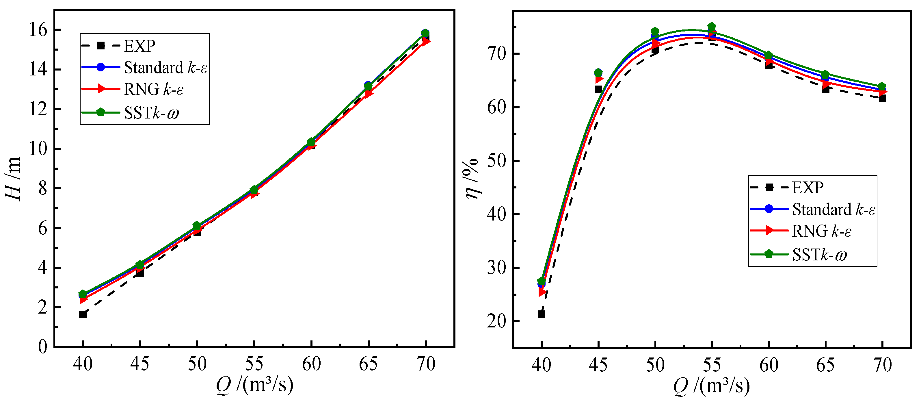
3.1. Experimental Validation of the Numerical Scheme

Existing turbulence models featured with ANSYS Fluent are Standard k-ε, RNG k-ε, SST k-ω, etc. Different turbulence models are suitable for different flow situations and need to be selected according to the actual situation. On that account, the performance of different turbulence models has been numerically assessed and compared with experimental results under flow rates ranging from 0.7 Q–1.2 Q. As illustrated by Figure 5, the numerical results of the RNG k-ε turbulence model mostly fall in good agreement with the experimental results. Therefore, the RNG k-ε turbulence model is the best option for this specific numerical simulation. In the range of 40–70 m³/s; the maximum relative errors of pump head and efficiency between experiment and numerical results are 1.60% and 2.89%, respectively. Hence, both the selected mesh arrangement and numerical methods can be considered reliable enough to guarantee the accuracy and reliability of numerical outcomes.

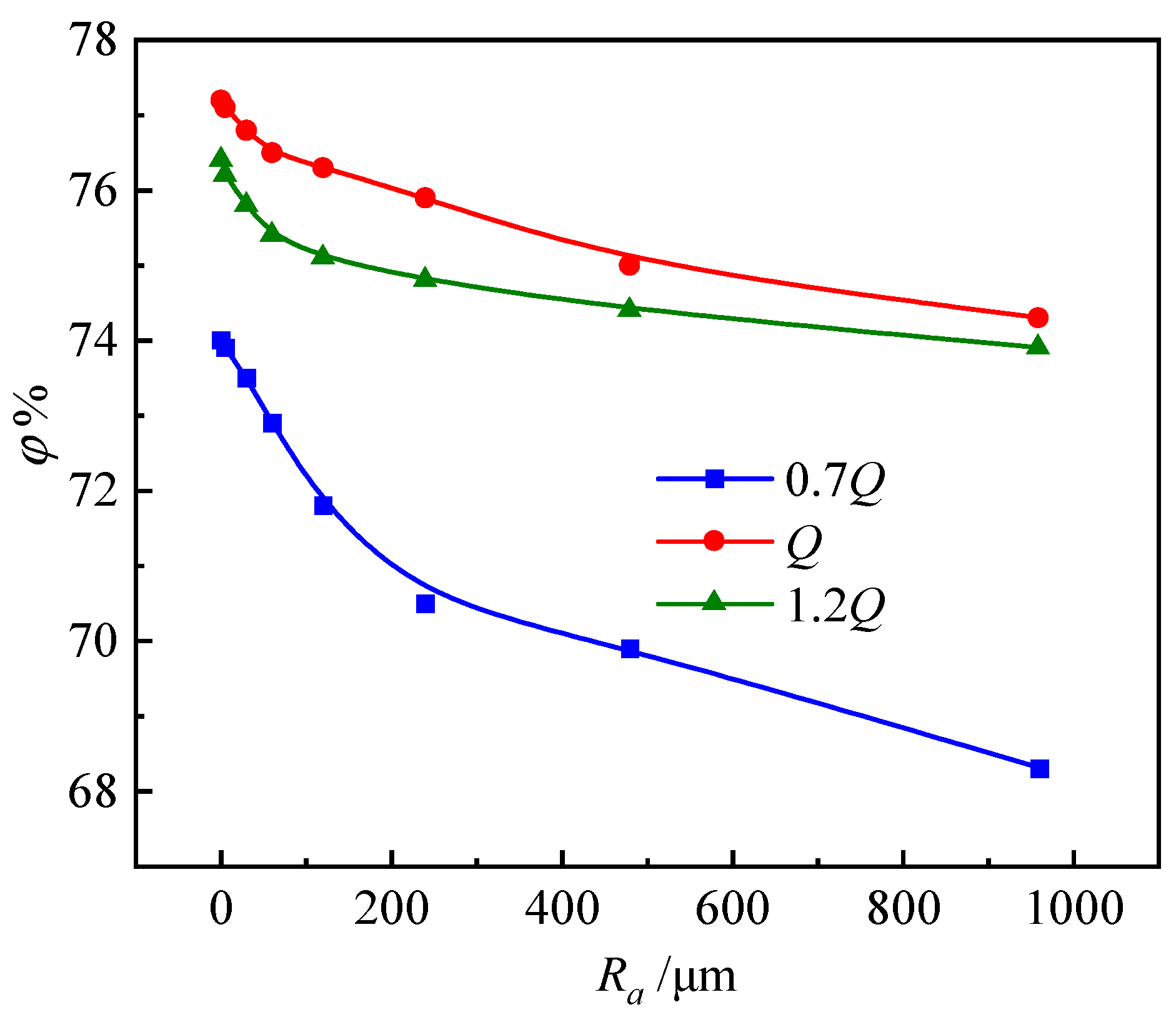
3.2. Effect of Wall Roughness on PAT Performance

For analytical purpose, the actual situation of the slanted axial flow PAT is simplified by modeling the wall roughness as a uniform distribution throughout the hydraulic components. To study the effect of the wall roughness on the slanted axial flow pump performance, different values of the wall roughness (R_a = 0 μm, 6 μm, 60 μm, 120 μm, 240 μm, 480 μm, 960 μm) are selected for the numerical calculation. For each wall roughness, Figure 6a,b show the corresponding performance characteristics (head and efficiency) variation with respect to the activated flow rate. The general remark for both figures is that the order of roughness influence on the head and efficiency for each flow rate is directly connected to the level of roughness; i.e., the deeper the roughness, the higher the performance reduction.

As to normal flow behavior, Figure 6a shows the proportionality between the flow rate and the head. That is, the increase of flow rate is concomitant to the head rise. The optimal condition of the investigated axial flow PAT is Q = 55 m³/s. When the flow rate is in the range of 0.7 Q–1.2 Q, the head at the same working point decreases gradually with the increase in wall roughness. When wall roughness increases from 0–960 μm, the head in each flow rate condition decreases by 21.0%, 14.6%, 9.9%, 7.9%, 9%, 6.9%, and 5% respectively. This demonstrates wall roughness has the maximum effect on pump head at the small flow rate condition, and the effect gradually decreases with increasing flow rate.

For all roughness scenarios in Figure 6b, it is clear that with the increase in flow rate, the efficiency displays an overall trend of increasing and decreasing before and after the optimum condition, respectively. In the range of 0.7 Q–1.2 Q, the efficiency gradually decreases with the increase in wall roughness at the same flow rate. When wall roughness increases from 0–960 μm, the efficiency in each of flow conditions decreases by 12.53%, 5.31%, 4.76%, 2.07%, and 5.72%, respectively. This shows that the wall roughness has the least effect on PAT performance at the optimal operating condition, while it inflicts a greater impact on PAT performance under off-design operating conditions, especially under low flow conditions. Therefore, the influence of wall roughness on the performance of an axial-flow PAT should be considered when the machine has been operating under off-design conditions for a long time.

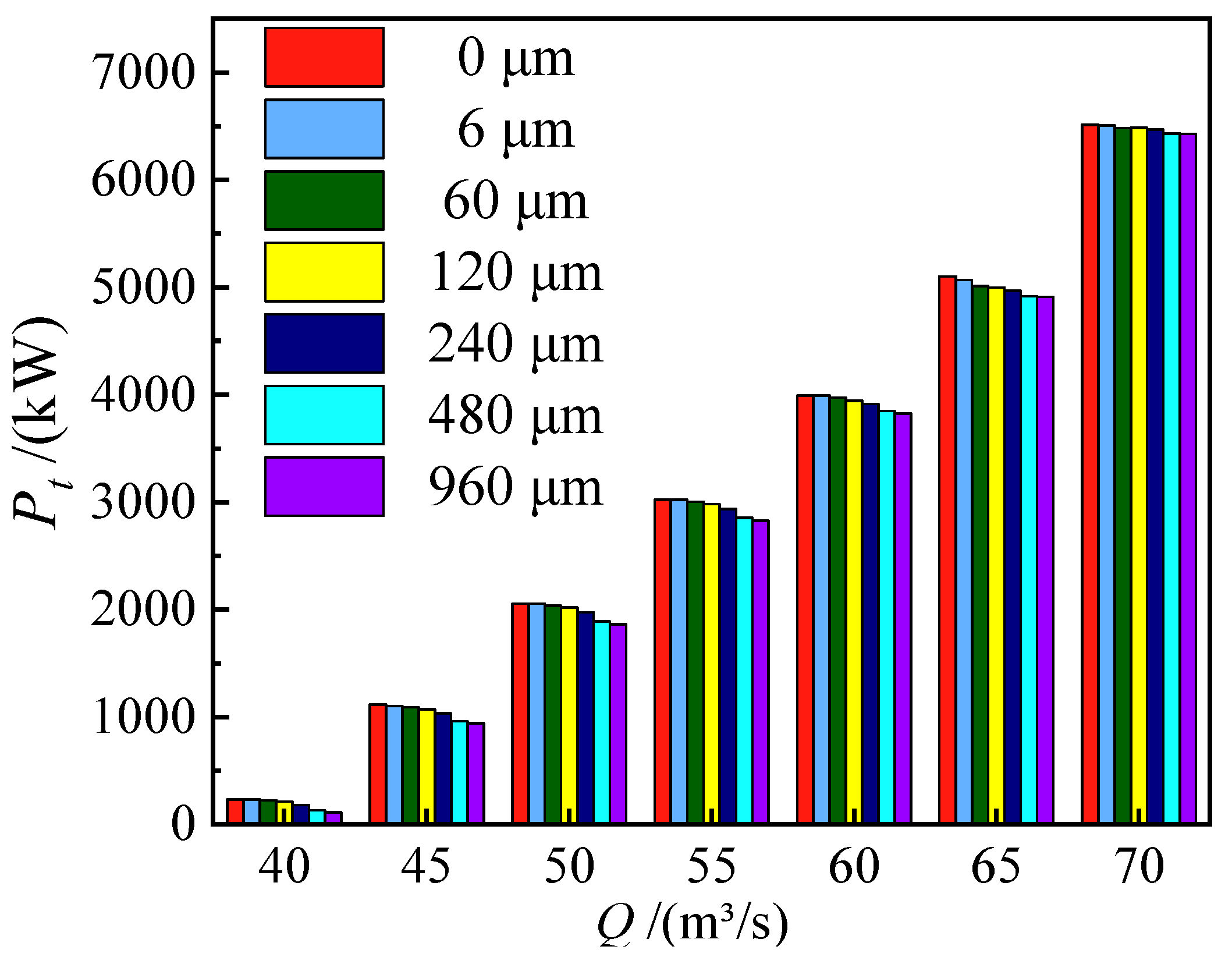
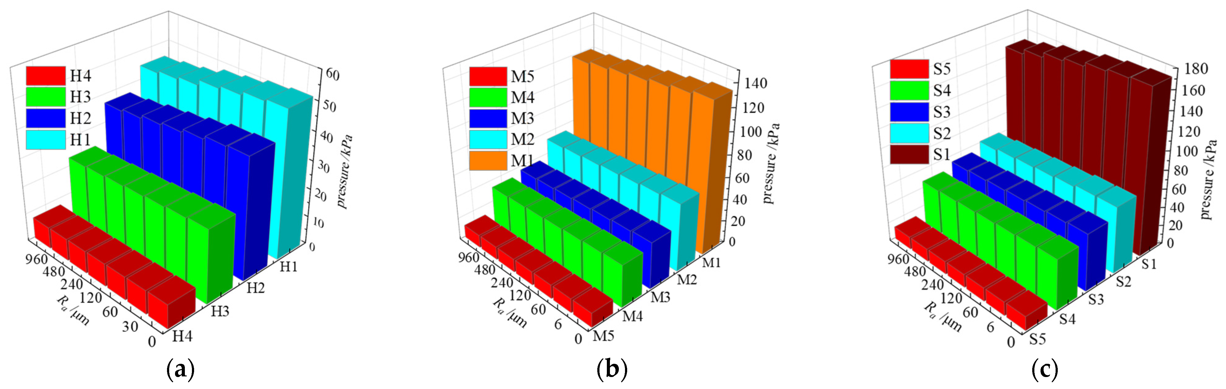
3.3. Effect of Wall Roughness on Shaft Power

Having demonstrated the direct influence of the wall roughness on the head and efficiency, it is reasonable to anticipate its impact on the shaft power, as well. Figure 7 shows the effect of different wall roughness depths on PAT’s shaft power (P_t) under different flow conditions. As noticed previously (Figure 6), the increase in flow rate corresponds to the same increase in the power of the water flow doing work on the impeller, which actuates the shaft power continuously. Once more, the extent of the wall roughness tends to have the same influence on the shaft power. This is evidenced while considering each flow rate alone; the shaft power displays a gradually decreasing pattern with the increasing wall roughness depth.

When the wall roughness increases from 0–960 μm, the shaft power for each of the investigated flow conditions correspondingly decreases by 50.5%, 15.6%, 9.3%, 6.5%, 4.2%, 3.7%, and 1%. It is therefore obvious that the effect of wall roughness on the shaft power is most significant under low flow conditions (Q = 40 m³/s), whereas it gradually weakens with further flow rate increase. Reflecting back to Figure 6, the roughness influence on the head is relatively small at the small flow rate, and wall roughness leads to greater shaft power decline. This corresponds to the main reason for the efficiency reduction at small flow rates.

3.4. Effect of Wall Roughness on Internal Flow

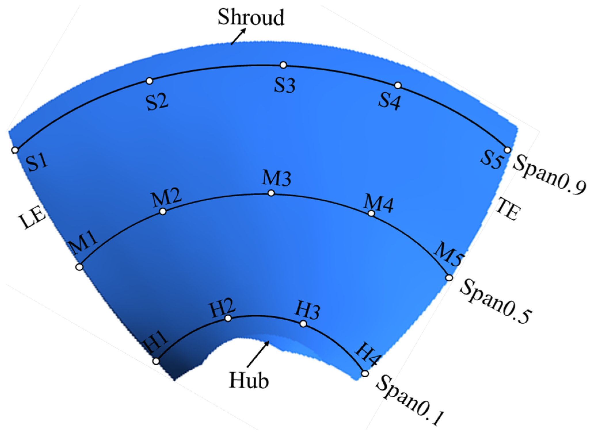
3.4.1. Wall Roughness Effect on Relative Flow Velocity over the Blade Pressure Surface

While investigating the wall roughness effect on the performance of a slanted axial flow PAT, the impact on the internal flow must be regarded as a key focus. For that purpose, monitoring points have been placed over the blade pressure surface along 3 lines at a span of 0.9, 0.5, and 0.1, respectively. As illustrated by Figure 8, equidistant 5 monitoring points (designated by “S”) are evenly arranged along the outermost chord direction of the blade and along the mid-span (designated by “M”), whereas 4 monitoring points (designated by “H”) have been evenly arranged over the innermost span.

As already found, the size of wall roughness has a proportional impact on machine performance. The same observation can be deduced from Figure 9 that shows the relative velocity (V_t) histograms of monitoring points (H3, M4, and S4) aligned radially from hub to shroud on the blade pressure surface. The outstanding observation is that as the relative velocity gets high towards outermost spans, the wall roughness keeps reducing the relative velocity according to its size. As tabulated in

Table 3. Relative velocity and percentages with different roughness.

Ra (μm)	H3		M4		S5
	Vr (m/s)	Relative Deviation (%)	Vr (m/s)	Relative Deviation (%)	Vr (m/s)	Relative Deviation (%)
0	8.13		14.04		22.62
6	8.06	0.87%	13.73	2.23%	22.42	0.89%
60	7.91	2.75%	13.34	4.98%	21.81	3.58%
120	7.55	7.15%	12.90	8.13%	21.16	6.45%
240	7.31	10.14%	12.47	11.21%	20.36	10.01%
480	7.22	11.23%	12.16	13.41%	19.83	12.34%
960	7.13	12.30%	11.89	15.31%	19.42	14.12%

, the relative velocity of roughness R_a = 0 μm at H3 is 8.134 m/s, which is 0.87%, 2.75%, 7.15%, 10.14%, 11.23%, 12.3% higher than that of wall roughness R_a = 0 μm, 60 μm, 120 μm, 240 μm, 480 μm, and 960 μm, respectively. The relative velocity of M4 roughness R_a = 0 μm is 14.04 m/s, which is 2.23%, 4.98%, 8.13%, 11.21%, 13.41%, 15.31% higher than that of R_a = 0 μm, 60 μm, 120 μm, 240 μm, 480 μm, and 960 μm, respectively. The relative velocity of S4 roughness R_a = 0 μm is 22.62 m/s, which is 0.89%, 3.58%, 6.45%, 10.01%, 12.34%, 14.12% higher than that of R_a = 0 μm, 60 μm, 120 μm, 240 μm, 480 μm, 960 μm, respectively. It can be seen that the relative velocity of the impeller blade pressure surface increases continuously along the radial direction. As the wall roughness of the impeller shroud, the friction resistance in the boundary layer increases. This results in energy loss increase and a decrease in the relative velocity of the impeller blade.

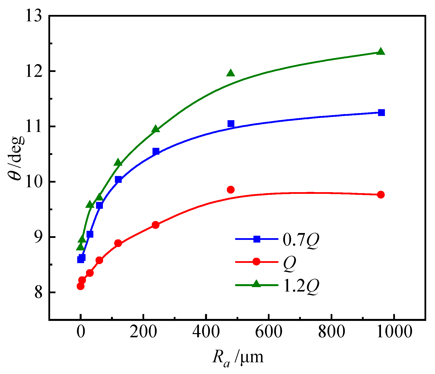
3.4.2. Effect of Wall Roughness on Impeller Outlet Flow

In order to study the effect of wall roughness on the impeller outlet flow field, the distribution uniformity of the axial velocity component ($\phi$) and velocity-weighted average swirl angle (θ) under different working conditions are analyzed. There is hardly any hydraulic loss when flow state at the impeller outlet is better. That is, when the axial velocity uniformity is around 100% and the velocity-weighted average swirl angle is smaller. $\phi$ and θ are calculated according to Equations (9) and (10), respectively.

$$\phi =[1-\frac{1}{V\mathrm{a}}\sqrt{{\displaystyle \sum _{i=1}^n[(Vai-Va)]}}]\times 100\%$$

(9)

$$\theta ={\displaystyle \sum _{i=1}^{n}V\mathrm{ai}}\left\{90°{-\mathrm{tg}}^{-1}\frac{Vti}{Vai}\right\}\backslash {\displaystyle \sum _{i=1}^{n}Vai}$$

(10)

where, $\phi$ is the distribution uniformity of axial velocity at the outlet section (%); V_a is the arithmetic average value of the axial velocity of outlet section (m/s); V_ai is the axial velocity (m/s) of each computing unit (representing each element) at the outlet section; θ is velocity-weighted average swirl angle (deg) of flow at outlet section; V_ti is the transverse velocity (m/s) of each calculation unit in the outlet section; n is the number of computing units on the exit section [30].

Figure 10 shows the curve of uniformity distribution for the axial flow velocity subjected to the variation of roughness under different working conditions. At first glance, the common trend of decreasing axial velocity uniformity with increasing wall roughness can be easily noticed. Under the optimal conditions (Q), the axial velocity distribution uniformity is excellent; i.e., it reaches its highest value, where the roughness-free wall displays a perfect uniformity. However; with the increase of roughness up to 960 μm, the axial velocity uniformity ($\phi$) decreases from 77.2 to 74.3%, which corresponds to an overall downward shift rate of about 2.9%. For small flow rate (0.7 Q), when the roughness increases up to 960 μm, the axial velocity uniformity ($\phi$) decreases from 74 to 68.3%, which is equivalent to the overall downward shift rate of about 5.7%. For large flow rate (1.2 Q), when the wall roughness increases up to 960 μm, the axial velocity distribution uniformity ($\phi$) decreases from 76.4 to 73.9%, which sums up to an overall downward shift rate of about 2.5%.

It can be seen that, under the reverse power generation condition of the slanted axial flow pump device, the increase in wall roughness leads to a decrease in the uniformity of axial velocity distribution. At the small flow rate of Q = 40 m³/s, wall roughness has the most significant effect on uniformity of axial velocity distribution, while the effect of wall roughness on uniformity of axial velocity distribution becomes minimal under the large flow rates. In light of previous findings, the low axial velocity uniformity may be one among several reasons that lead to the low operation efficiency of reverse power generation under the small flow conditions.

Another parameter to evaluate the wall roughness effect on impeller outlet flow is the velocity-weighted average swirl angle. Figure 11 portrays its variation in terms of wall roughness stretch under different working conditions. Under different flow rates, the curve outline of the velocity-weighted average swirl angle closely reproduces the same shape similarity. The common inference is that the velocity-weighted average swirl angle is unambiguously associated to the wall roughness size.

Under the optimal conditions (Q), the velocity-weighted average swirl angle is at its minimum value, no matter the wall roughness. The increase in wall roughness (0–960 μm) at that best efficiency operation results into the slightest increase of the velocity-weighted average swirl angle of 1.66° (8.1° up to 9.76°). Under the small flow rate (0.7 Q), 0–960 μm increase of wall roughness give rise to 8.59–11.25° increase in the velocity weighted average swirl angle (2.66° increment). Under the small flow rate (0.7 Q), the same wall roughness increase brings about 3.46° increases (8.88–12.34°) in the velocity weighted average swirl angle. Hence, the increase in wall roughness leads to the increase in velocity-weighted average swirl angle; and the maximum velocity-weighted average swirl angle is obtained under large flow conditions. With reference to the discussion beforehand, the high velocity-weighted average swirl angle may be one of reasons that lead to the low operational efficiency of reverse power generation under the large flow conditions.

3.4.3. Effect of Wall Roughness on Streamline of Outlet Conduit

Streamline at the exit is another aspect to evidence the wall roughness impact on the machine performance. Figure 12 shows the three-dimensional streamlines of the outlet conduit under different flow conditions when the slanted axial flow pump device is used for reverse power generation. Only, three values of wall roughness (R_a = 0 μm, 240 μm, and 960 μm) have been selected for comparative analysis. It can be found that with the increase in wall roughness, the streamlines of the outlet conduit grow disordered.

Under the small flow rates of 0.7 Q, streamlines in the outlet conduit are smooth and less swirling flow appears. This is obviously remarkable within moderate roughness size of R_a = 0 μm and 240 μm. Conversely, backflow phenomena relatively occur in the outlet conduit at higher flow rate (1.2 Q), and they become clearer at a deeper wall roughness (R_a = 960 μm). Under the optimal condition, the flow state in the outlet conduit has minor variation with increasing wall roughness. Thus, the wall roughness has the least influence on the streamline state of the slanted axial flow PAT within such best efficiency operations. Under large flow rates (R_a = 240 μm and 960 μm), the flow state in the outlet conduit becomes worse than that with the smooth wall. With the increase in wall roughness, the flow state in the outlet conduit becomes obviously worse; obvious vortex and backflow phenomena grow quite apparent. In conclusion, swirl flow of the outlet conduit becomes significant when the velocity-weighted average swirl angle at the large flow rate is high with rough surface.

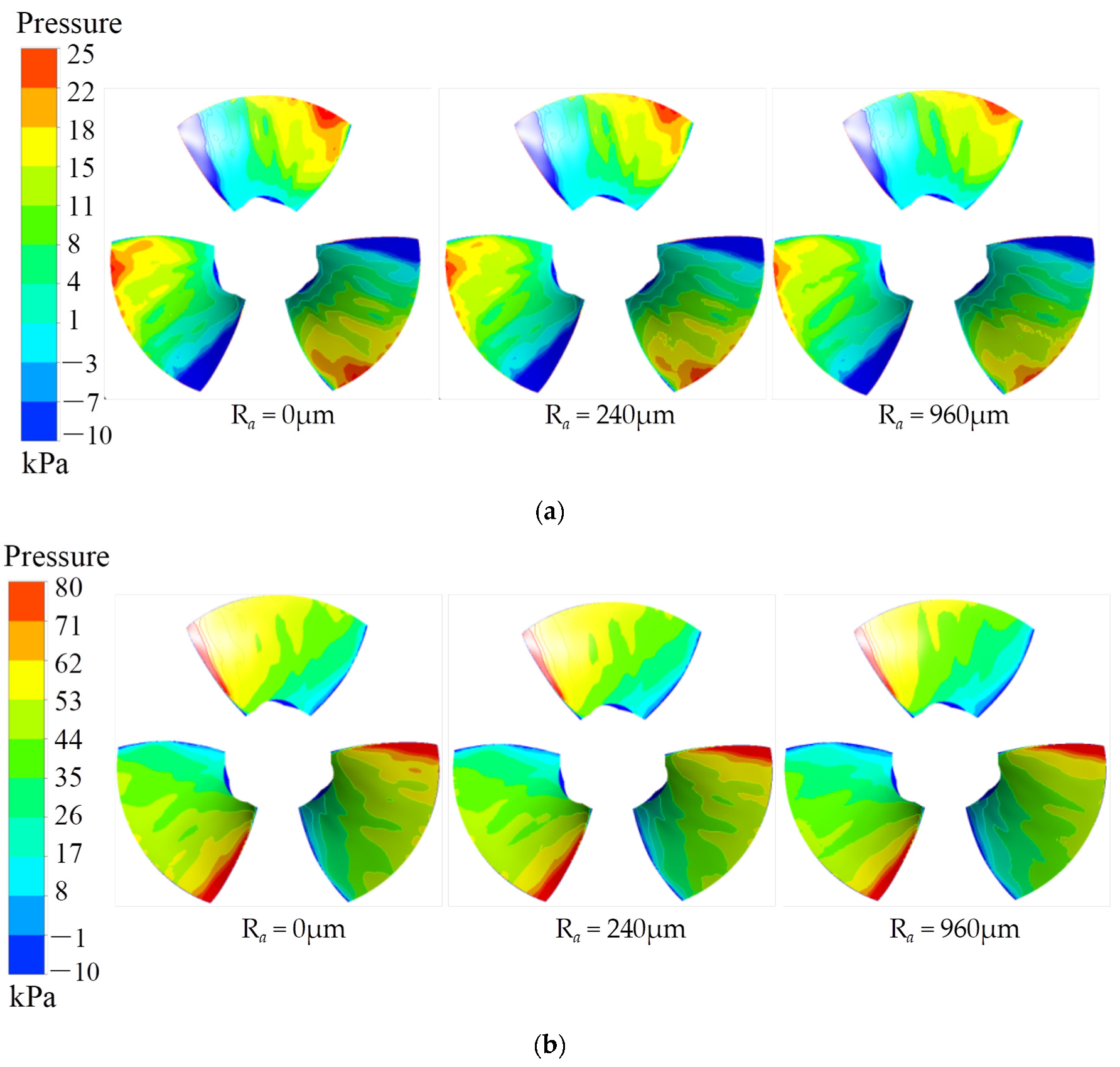
3.4.4. Effect of Wall Roughness on Pressure Distribution over the Blade Pressure Surface

Figure 13 shows the distribution of pressure on blade pressure surface with a changing wall roughness. The pressure on the blade surface obviously varies with a high gradient along the chord direction of the blade, especially at large flow rate. Under the small flow rate, a local low pressure area appears near the leading edge, it increases gradually along the chord direction of the blade, and a local high pressure appears near the impeller shroud of the trailing edge, while there is an opposite variation trend under the larger flow rates.

The negative pressure on the blade is more likely to result in cavitation, which can lead to an increase of wall roughness. At the same flow rate, the negative pressure area becomes larger with the increase of wall roughness. Under the same wall roughness, the negative pressure decreases with the increase of flow rate and the positive pressure increase with the increase in wall roughness. Therefore, the increase of wall roughness easily causes cavitation. In the vicinity of the leading edge, the range of high pressure zone is the largest at the large flow rate, followed by rated flow rate, and the high pressure zone is not obvious at the small flow rate.

Figure 14 shows the variation of pressure at the monitoring point of blade pressure surface with wall roughness under the optimal condition. It can be seen from the figure that with the increase of wall roughness, the pressure decreases gradually, resulting in an increase of energy loss near the boundary layer [31]. In the radial direction (from hub to shroud), the pressure increases gradually.

Table 4. Relative deviation from 0 μm to 960 μm (%).

	Span0.1				Span0.5					Span0.9
Point	H1	H2	H3	H4	M1	M2	M3	M4	M5	S1	S2	S3	S4	S5
Deviation (%)	11	8	14	13	11	5.2	3.6	3.2	1.1	11	14	13	11	15

shows relative deviation of pressure from 0 μm to 960 μm of monitoring points at different spans. Near the hub, at R_a = 960 μm, the pressure of H1, H2, H3, and H4 is 7752 Pa, 23,318 Pa, 37,201 Pa, and 45,172 Pa, respectively. From Table 4, compared with the smooth wall; the pressure decreases by 11%, 8%, 14%, and 13%, respectively. In the middle of the blade, at R_a = 960 μm, the pressures of M1, M2, M3, M4, and M5 are 119,776 Pa, 54,349 Pa, 37,484 Pa, 34,061 Pa, and 11,626 Pa, respectively, compared with smooth wall, the pressures decrease by 11.4%, 5.2%, 3.6%, 3.2%, and 1.1%, respectively. The pressure of the monitoring point M1 under the smooth wall surface is 135,212 Pa. At R_a = 6 μm, 60 μm, 120 μm, 240 μm, 480 μm, and 960 μm, the pressure of M1 decreases by 1.3%, 2.5%, 4.5%, 7.2%, 8.9%, and 11.4% compared with the smooth wall surface. It indicates that when the roughness is greater than 240 μm, the roughness has a great influence on the pressure near the trailing edge. The pressure of M2, M3, and M4 monitoring points has a similar trend with roughness to that of M1. The minimum pressure value at M5 point under the smooth wall is 13,547 Pa. With the increasing wall roughness, the pressure decreases by 0.36%, 0.12%, 3.5%, 7%, 8.5%, 13.5%, and 18.3%, respectively. It can be seen that when the roughness is less than 60 μm, the roughness has little influence on the pressure near the leading edge. From Figure 12c, at R_a = 960 μm, the pressures of S1, S2, S3, S4, and S5 are 151,730 Pa, 59,123 Pa, 51,258 Pa, 45, 943 Pa, and 12,476 Pa, respectively, compared with smooth wall, the pressures decrease by 11%, 14%, 13.2%, 10.8%, and 15%, respectively. It demonstrates that the wall roughness has a great influence on pressure of the blade near the impeller shroud. The results indicate that the boundary layer flow is obviously affected by wall roughness and pressure losses increase significantly due to wall roughness.

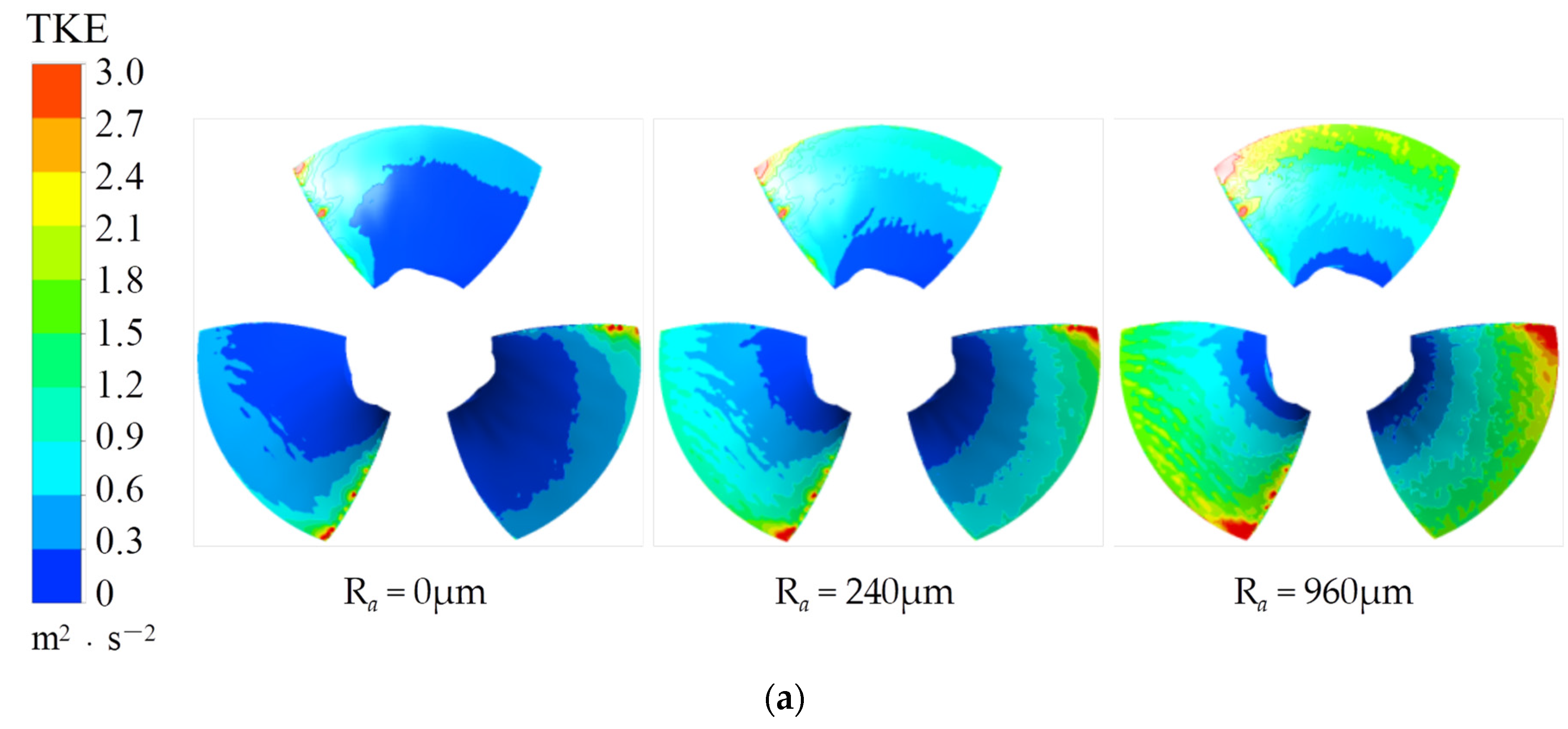
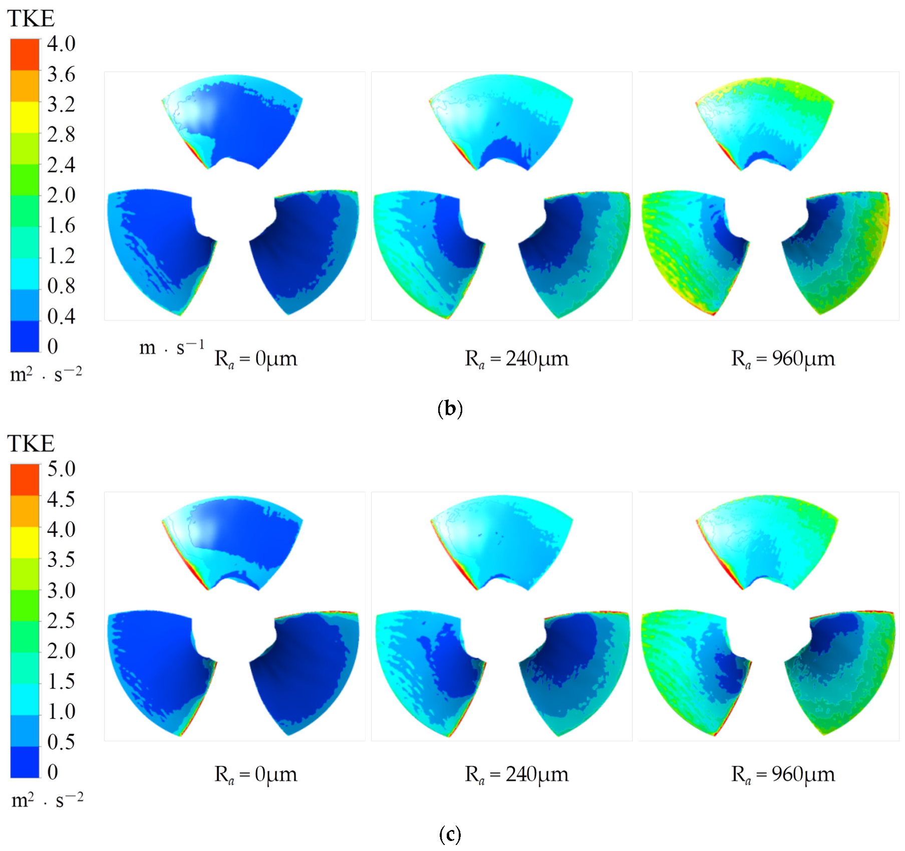
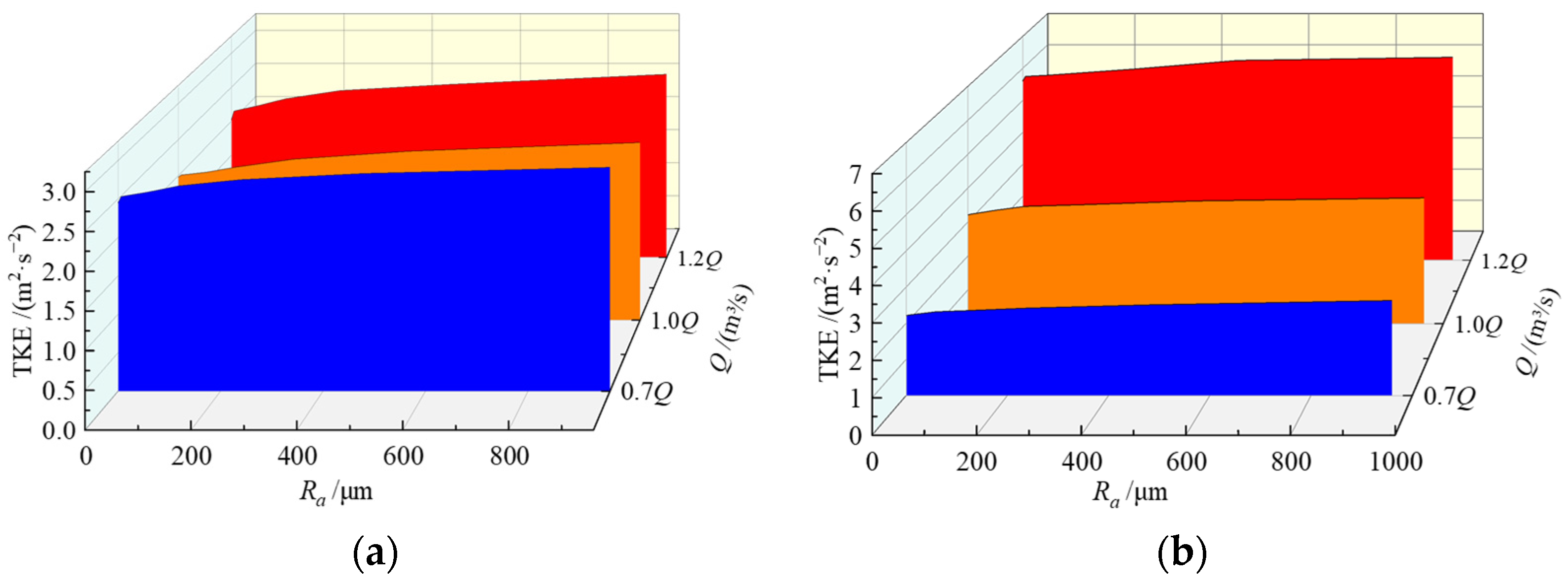
3.4.5. Effect of Wall Roughness on Turbulent Kinetic Energy

Turbulent kinetic energy (TKE) is a measure of the turbulence intensity, associated with momentum transport through turbulence eddies in the boundary layer region [32]. The distribution of turbulent kinetic energy on the blade pressure surface is shown in Figure 15. The values of wall roughness of 0 μm, 240 μm, and 960 μm are taken. It can be seen from the figure that, under the same flow condition, the TKE increases with the increase of roughness, especially near the impeller shroud. Under the small flow rate, the TKE near the impeller shroud is obviously higher. Under the optimal condition, when the wall gradually changes from smooth to rough, the TKE is obviously stronger along the radial direction and the distribution range of the TKE increases. The effect of roughness on TKE is more obvious at the large flow rate.

The distribution of TKE on the blade suction surface is shown in Figure 16. As can it be seen from the figure, the TKE on the suction surface of the blade is larger than that on the pressure surface of the blade under the small flow rate, and the TKE is strengthened near the impeller shroud. Under optimal conditions and large flow conditions, the TKE near the leading edge of the blade increases; this is more obvious under the large flow rate. Under different flow conditions, the distribution range and magnitude of TKE on the blade suction surface increase with the increase in wall roughness.

The TKE of blade surface under different working conditions is shown in Figure 17. It can be seen that the TKE gradually increases with the increase in wall roughness, which leads to the increase of energy loss near the boundary layer and is also one of the important reasons for the decrease in efficiency of the slanted axial flow PAT. In each working condition, the TKE of the blade surface increases gradually with the increase in wall roughness, but the variation amplitude is small. When the wall roughness is the same, the TKE of the pressure surface varies little with the flow rate. While the TKE of the suction surface changes obviously with the flow rate and increases significantly with the increase of the flow rate.

4. Conclusions

The slanted axial flow PAT operated under turbine mode has been, in this study, numerically simulated. Specifically, the investigation target was the influence of different wall roughness depths on both the external performance and internal flow field characteristics under different working conditions. From narrated findings and pertinent discussion, a number of concluding remarks can be drawn as follows:

(1)

Under constant individual flow rates, the gradual deterioration of PAT performance (measured through parameters such as the hydraulic efficiency, head, and shaft power) is conspicuously associated with the increase in wall roughness depth. The later displays a minimum impact on PAT performance only under optimal flow conditions, while for off-design flow conditions, the larger the deviation from the best efficient point, the greater the impact on PAT performance characteristics.

(2)

Under turbine operating mode, the increase of wall roughness simultaneously brings about a messy non-uniform distribution of axial velocity and an increase of the velocity-weighted average swirl angle. Furthermore, streamlines within the discharge conduit reflect a disorderly flow pattern, eventually giving rise to backflow structures.

(3)

Ultimately, the wall roughness accumulation remarkably triggers the increase of energy losses. This is evidenced by the drop of static pressure on the blade pressure surface and the increase of TKE on the blade. The latter is particularly evident near the impeller shroud. Under the same roughness conditions, the TKE on the blade suction surface proves to be greater than that on the blade pressure surface.

Given the level of PAT performance degradation that can be caused by the machine wall roughness, future research endeavors are encouraged in this field, where the effects of wall roughness can be investigated further and a wider range of machine operating conditions and roughness depths can be considered. This would help monitoring PAT’s lengthy operations and assist the timely equipment refurbishment or replacement without highly impairing the machine performance.

References

1. Yang, F.; Li, Z.; Hu, W.; Liu, C.; Jiang, D.; Liu, D.; Nasr, A. Analysis of flow loss characteristics of slanted axial-flow pump device based on entropy production theory. R. Soc. Open Sci. 2022, 9, 211208. [Google Scholar] [CrossRef] [PubMed]
2. Kan, K.; Yang, Z.; Lyu, P.; Zheng, Y.; Shen, L. Numerical study of turbulent flow past a rotating axial-flow pump based on a level-set immersed boundary method. Renew. Energy 2021, 168, 960–971. [Google Scholar] [CrossRef]
3. Shi, L.; Zhang, W.; Jiao, H.; Tang, F.; Wang, L.; Sun, D.; Shi, W. Numerical simulation and experimental study on the comparison of the hydraulic characteristics of an axial-flow pump and a full tubular pump. Renew. Energy 2020, 153, 1455–1464. [Google Scholar] [CrossRef]
4. Shi, L.; Yuan, Y.; Jiao, H.; Tang, F.; Cheng, L.; Yang, F.; Jin, Y.; Zhu, J. Numerical investigation and experiment on pressure pulsation characteristics in a full tubular pump. Renew. Energy 2021, 163, 987–1000. [Google Scholar] [CrossRef]
5. Liu, Y.; Tan, L. Tip clearance on pressure fluctuation intensity and vortex characteristic of a mixed flow pump as turbine at pump mode. Renew. Energy 2018, 129, 606–615. [Google Scholar] [CrossRef]
6. Kan, K.; Zhang, Q.; Xu, Z.; Zheng, Y.; Gao, Q.; Shen, L. Energy loss mechanism due to tip leakage flow of axial flow pump as turbine under various operating conditions. Energy 2022, 255, 124532. [Google Scholar] [CrossRef]
7. Yang, S.S.; Derakhshan, S.; Kong, F.Y. Theoretical, numerical and experimental prediction of pump as turbine performance. Renewable. Energy 2012, 48, 507–513. [Google Scholar] [CrossRef]
8. Jain, S.V.; Patel, R.N. Investigations on pump running in turbine mode: A review of the state-of-the-art. Renew. Sustain. Energy Rev. 2014, 30, 841–868. [Google Scholar] [CrossRef]
9. Aldaş, K.; Yapıcı, R. Investigation of effects of scale and surface roughness on efficiency of water jet pumps using CFD. Eng. Appl. Comput. Fluid Mech. 2014, 8, 14–25. [Google Scholar] [CrossRef] [Green Version]
10. Han, Y.; Tan, L. Influence of rotating speed on tip leakage vortex in a mixed flow pump as turbine at pump mode. Renew. Energy 2020, 162, 144–150. [Google Scholar] [CrossRef]
11. Lin, T.; Zhu, Z.; Li, X.; Li, J.; Lin, Y. Theoretical, experimental, and numerical methods to predict the best efficiency point of centrifugal pump as turbine. Renew. Energy 2021, 168, 31–44. [Google Scholar] [CrossRef]
12. Sun-Sheng, Y.; Fan-Yu, K.; Jian-Hui, F.; Ling, X. Numerical research on effects of splitter blades to the influence of pump as turbine. Int. J. Rotating Mach. 2012, 2012, 123093. [Google Scholar] [CrossRef] [Green Version]
13. Capurso, T.; Bergamini, L.; Camporeale, S.M.; Fortunato, B.; Torresi, M. CFD analysis of the performance of a novel impeller for a double suction centrifugal pump working as a turbine. In Proceedings of the 13th European Conference on Turbomachinery Fluid dynamics & Thermodynamics. European Turbomachinery Society, Lausanne, Switzerland, 24–28 April 2019. [Google Scholar]
14. Derakhshan, S.; Mohammadi, B.; Nourbakhsh, A. Efficiency improvement of centrifugal reverse pumps. J. Fluids Eng. 2009, 131, 021103. [Google Scholar] [CrossRef]
15. Morabito, A.; Vagnoni, E.; Di Matteo, M.; Hendrick, P. Numerical investigation on the volute cutwater for pumps running in turbine mode. Renew. Energy 2021, 175, 807–824. [Google Scholar] [CrossRef]
16. Gülich, J.F. Effect of Reynolds number and surface roughness on the efficiency of centrifugal pumps. J. Fluids Eng. 2003, 125, 670–679. [Google Scholar] [CrossRef]
17. Bai, T.; Liu, J.; Zhang, W.; Zou, Z. Effect of surface roughness on the aerodynamic performance of turbine blade cascade. Propuls. Power Res. 2014, 3, 82–89. [Google Scholar] [CrossRef] [Green Version]
18. Bellary, S.A.I.; Samad, A. Exit blade angle and roughness effect on centrifugal pump performance. In Proceedings of the Gas Turbine India Conference, Bangalore, Karnataka, 5–6 December 2013; American Society of Mechanical Engineers: New York, NY, USA; pp. 1–10. [Google Scholar]
19. Deshmukh, D.; Samad, A. CFD-based analysis for finding critical wall roughness on centrifugal pump at design and off-design conditions. J. Braz. Soc. Mech. Sci. Eng. 2019, 41, 1–18. [Google Scholar] [CrossRef]
20. Juckelandt, K.; Bleeck, S.; Wurm, F.H. Analysis of losses in centrifugal pumps with low specific speed with smooth and rough walls. In Proceedings of the 11th European Conference on Turbomachinery Fluid dynamics & Thermodynamics, European Turbomachinery society, Madrid, Spain, 23–27 March 2015. [Google Scholar]
21. He, X.; Jiao, W.; Wang, C.; Cao, W. Influence of surface roughness on the pump performance based on Computational Fluid Dynamics. IEEE Access 2019, 7, 105331–105341. [Google Scholar] [CrossRef]
22. Limbach, P.; Skoda, R. Numerical and experimental analysis of cavitating flow in a low specific speed centrifugal pump with different surface roughness. J. Fluids Eng. 2017, 139, 101201. [Google Scholar] [CrossRef]
23. Lim, S.E.; Sohn, C.H. CFD analysis of performance change in accordance with inner surface roughness of a double-entry centrifugal pump. J. Mech. Sci. Technol. 2018, 32, 697–702. [Google Scholar] [CrossRef]
24. Kan, K.; Xu, Z.; Chen, H.; Xu, H.; Zheng, Y.; Zhou, D.; Muhirwa, A.; Maxime, B. Energy loss mechanisms of transition from pump mode to turbine mode of an axial-flow pump under bidirectional conditions. Energy 2022, 257, 124630. [Google Scholar] [CrossRef]
25. Kan, K.; Chen, H.; Zheng, Y.; Zhou, D.; Binama, M.; Dai, J. Transient characteristics during power-off process in a shaft extension tubular pump by using a suitable numerical model. Renew. Energy 2021, 164, 109–121. [Google Scholar] [CrossRef]
26. He, X.; Zhang, Y.; Wang, C.; Zhang, C.; Cheng, L.; Chen, K.; Hu, B. Influence of critical wall roughness on the performance of double-channel sewage pump. Energies 2020, 13, 464. [Google Scholar] [CrossRef] [Green Version]
27. Shockling, M.A.; Allen, J.J.; Smits, A.J. Roughness effects in turbulent pipe flow. J. Fluid Mech. 2006, 564, 267–285. [Google Scholar] [CrossRef]
28. Adams, T.; Grant, C.; Watson, H. A simple algorithm to relate measured surface roughness to equivalent sand-grain roughness. Int. J. Mech. Eng. Mechatron. 2012, 1, 66–71. [Google Scholar] [CrossRef] [Green Version]
29. Ji, L.; Li, W.; Shi, W.; Tian, F.; Agarwal, R. Diagnosis of internal energy characteristics of mixed-flow pump within stall region based on entropy production analysis model. Int. Commun. Heat Mass Transf. 2020, 117, 104784. [Google Scholar] [CrossRef]
30. Sha, L.; Yang, S.; Kong, X.; Sun, H.; Pei, L. Influence of inlet flow field uniformity on the performance of the nuclear main pump. IOP Conf. Ser. Mater. Sci. Eng. 2021, 1081, 012024. [Google Scholar] [CrossRef]
31. Skrzypacz, J.; Bieganowski, M. The influence of micro grooves on the parameters of thecentrifugal pμmp impeller. Int. J. Mech. Sci. 2018, 144, 827–835. [Google Scholar] [CrossRef]
32. Li, W.; Ji, L.; Li, E.; Shi, W.; Agarwal, R.; Zhou, L. Numerical investigation of energy loss mechanism of mixed-flow pump under stall condition. Renew. Energy 2021, 167, 740–760. [Google Scholar] [CrossRef]
Figure 1. Equivalent sand-grain roughness (a) and the surface profile diagram (b).
Sustainability 14 08459 g001
Figure 2. Computational domain of the axial flow PAT.
Sustainability 14 08459 g002
Figure 3. Unstructured mesh of the slanted axial flow pump components. (a)inlet conduit, guide vane (b) impeller, outlet conduit.
Sustainability 14 08459 g003
Figure 4. The grid independence assessment against the efficiency.
Sustainability 14 08459 g004
Figure 5. Experimental and numerical results with different turbulent models.
Sustainability 14 08459 g005
Figure 6. The slanted axial flow PAT performance varies with flow rate at different wall roughness. (a) Head variation with the flow rate (b) efficiency variation with the flow rate.
Sustainability 14 08459 g006
Figure 7. Shaft power varies with flow rate at different wall roughness.
Sustainability 14 08459 g007
Figure 8. Schematic diagram of monitoring points on blade pressure surface.
Sustainability 14 08459 g008
Figure 9. Effect of roughness on relative velocity on blade pressure surface.
Sustainability 14 08459 g009
Figure 10. Effect of roughness on axial velocity uniformity.
Sustainability 14 08459 g010
Figure 11. Effect of roughness on velocity-weighted average swirl angle.
Sustainability 14 08459 g011
Figure 12. Streamline of the outlet conduit under different flow rates. (a) 0.7 Q; (b) Q; (c) 1.2 Q.
Sustainability 14 08459 g012
Figure 13. Distribution of pressure on blade pressure surface. (a) 0.7 Q; (b) Q; (c) 1.2 Q.
Sustainability 14 08459 g013aSustainability 14 08459 g013b
Figure 14. Variation of pressure at the monitoring point with wall roughness. (a) span0.1 (b) span0.5 (c) span0.9.
Sustainability 14 08459 g014
Figure 15. The distribution of TKE on blade pressure surface. (a) 0.7 Q; (b) Q; (c) 1.2 Q.
Sustainability 14 08459 g015aSustainability 14 08459 g015b
Figure 16. The distribution of TKE on blade suction surface; (a) 0.7 Q; (b) Q; (c) 1.2 Q.
Sustainability 14 08459 g016
Figure 17. TKE of blade surface under different conditions. (a) TKE on blade pressure surface (b) TKE on blade suction surface.
Sustainability 14 08459 g017