Article

The Role of Education and Income Inequality on Environmental Quality: A Panel Data Analysis of the EKC Hypothesis on OECD Countries

by
Paolo Maranzano
1,*,
João Paulo Cerdeira Bento
2 and
Matteo Manera
1,3
1
Department of Economics, Management and Statistics (DEMS), University of Milano-Bicocca, Piazza dell’Ateneo Nuovo, 1, 20126 Milano, Italy
2
Department of Economics, Management, Industrial Engineering and Tourism (DEGEIT), Campus Universitário de Santiago, University of Aveiro, 3810-193 Aveiro, Portugal
3
Fondazione Eni Enrico Mattei (FEEM), Corso Magenta, 63, 20126 Milano, Italy
*
Author to whom correspondence should be addressed.
Sustainability 2022, 14(3), 1622; https://doi.org/10.3390/su14031622
Submission received: 10 January 2022 / Revised: 25 January 2022 / Accepted: 27 January 2022 / Published: 30 January 2022
(This article belongs to the Special Issue Sustainability and the Environmental Kuznets Curve Conjecture)

Abstract

:
This study examines the impact of education on the pollution–income relationship, controlling for income inequality in 17 European OECD countries over the period 1950–2015. We developed a novel two-stage algorithm, whose first step consists in applying clustering techniques to group countries according to the income inequality temporal pattern. In the second step, we estimate the educational-mitigated EKC hypothesis (Educational EKC) by employing panel regression techniques accounting for endogeneity issues. The clustering findings suggest the existence of high variability in income inequality levels across countries and heterogeneous development patterns. Empirical estimates highlight that, for high income inequality countries, the Educational EKC hypothesis holds, and that the emissions–income elasticity appears to decline when including the schooling level. In the low income inequality cluster, these effects are not clear-cut. For these countries, we propose a different specification of the EKC, which substitutes the income per capita term with the years of schooling. The new specification is statistically validated for both high income inequality and low income inequality countries. In conclusion, we can state that education should be addressed as a crucial cornerstone to shaping the EKC curve.
JEL Classification:
Q56; I24-25; C51-52; O15; O44

1. Introduction

The literature on the debate over growth and environmental issues is vast. Most studies refer to the evidence that there is a relationship between environmental quality and income, of the kind that environmental quality worsens at early periods of economic development and improves at later periods, as the economy develops. The literature on this relationship focuses on testing the Environmental Kuznets Curve, hereafter EKC, hypothesis [1,2].
This paper focuses on the importance of including education in the EKC modeling. We will use the average years of schooling as a proxy of human capital. Included in the panel dataset are all the OECD member states and we use a parabolic specification to model the EKC relationship. This paper discusses the role played by education and schooling in long-term development and its impact on the environment. The rationale is that the literature on the EKC has often debated on control variables to avoid omission bias, and has also modeled external factors that can negatively influence the quality of the environment, but rarely included any issue related to the role of human capital. Nevertheless, there is a study for Australia that has focused on how the educational level may affect the level of emissions within the EKC framework in the period from 1950 to 2015 [3]. Its finding is that education has played an essential role in economic development in the long run and, therefore, cannot be ignored within the pollution–income relationship.
What is expected from the empirical results on the relationship between pollution and schooling is the identification of a concave quadratic curve that grows in the initial phase and then decreases once the turning point has been passed. Analytically, the expectations lead to an inverted-U shape in addition to the main hypothesis underlying the EKC model. We refer to this result as the Educational EKC, which will be opposed to the economically driven specification commonly known as the Standard EKC. The concave shape can be justified interpreting education as a process moving along with the long-run economic development of countries. Historically, at an early stage of development, countries exhibit low levels of education and economic production. In the short run, the productive system invests in intensive industrial production, often supported by eco-unfriendly technologies and resources. Sustainable economic development requires a parallel and balanced strengthening of physical capital, technology, knowledge, and human capital to generate an extra boosting effect on the economy without wasting natural resources. In this phase, the economy needs to override the technological improvements brought about by knowledge. The turning point is reached when the educational system offers people the skills to develop efficient and environmentally compatible technologies and social instruments to adopt sustainable lifestyles. Hence, the human capital will push the economy towards more sustainable behaviors able to increase wealth and collective well-being simultaneously. Virtuous examples of these mechanisms are the countries of Central and Northern Europe, which show simultaneously very high levels of human capital and wealth.
As a further contribution, we consider as a discriminant factor the income inequality affecting the countries in the panel, as suggested by [4]. Using the Gini Index as a proxy of the social inequality, we aim at assessing whether the level of income inequality across countries affects the relationship between income, pollution, and level of schooling. First, we want to check if the estimated coefficients associated with income and education change in magnitude and statistical significance by considering countries all together and divided into groups based on their level of income inequality. Second, we assess whether the education variable has the same effect on environmental degradation in high income and low income inequality countries.
The remainder of the paper is structured as follows. In Section 2, we introduce the empirical specification of the EKC, augmented by the effect of the educational level, pointing out our expectations regarding the parameter values and their interpretation. In Section 3, we describe the available data and their sources. In Section 4, we describe the statistical methodologies implemented to test the research questions. In particular, we focus on the two-stage approach developed to estimate the effect of income inequality and schooling on CO2 emissions. In Section 5, we comment on the empirical results based on the OECD panel. In Section 6, we critically discuss the interpretation of the empirical evidence relative to the existing econometric literature and provide some suggestions for policymakers. Lastly, Section 7 sums up the contents of the paper.

2. Specification of Standard and Educational EKC

The specification of the Standard EKC model sets the per capita emission levels in a quadratic relationship with the per capita income, augmented by a set of control variables that capture indirect and external factors affecting the quality of the environment. Extending the proposal of Balaguer and Cantavella [3], in this paper we propose a panel specification of the Educational EKC which expresses the environmental quality as a quadratic function of both the per capita income and the educational level. According to a log-log panel specification, the model can be expressed as follows:
l o g ( C O 2 , i t / P o p i t ) = β 0 + β 1 l o g ( G D P i t / P o p i t ) + β 2 l o g ( G D P i t / P o p i t ) 2 + β 3 l o g ( S c h i t ) + β 4 l o g ( S c h i t ) 2 + Θ Z i t + ε i t
where C O 2 , i t / P o p i t refers to the per capita C O 2 emission levels, G D P i t / P o p i t is the per capita income, S c h i t is the educational level, measured as the average number of schooling years, Z i t is the set of control variables, and ε i t is the error term.
The Standard EKC hypothesis is supported by the data if β 1 > 0 , β 2 < 0 and the turning point T P i n c = e x p ( β 1 2 β 2 ) belongs to the observed range of per capita income values. The coefficients can be interpreted as elasticities since all the variables are expressed in a logarithmic scale. The empirical relationship between environmental quality and the level of education is modeled through a quadratic specification with coefficients β 3 and β 4 . The expected relationship between these variables is a quadratic inverted-U shape form, whose coefficients must respect the same sign constraints of the EKC hypothesis, i.e., β 3 > 0 and β 4 < 0 . The empirical turning point T P E D U = e x p ( β 3 2 β 4 ) identifies the minimum years of schooling such that pollution begins to decrease. In other words, it can be interpreted as the educational level that must be reached in order to guarantee long-term sustainable development.
The Kuznets Curve has been proposed by Simon Kuznets and is a hypothetical curve that graphs income inequality against income per capita over the course of the society’s urbanization and industrialization [5]. This relation has led to the development of the EKC [1,6]. As income increases, environmental pressure also grows to a certain point, and from that point the relationship becomes negative [7]. Moreover, as social welfare increases, people are more willing to use certified products and services complying with many environmental standards. The improvement in the quality of life leads society to put pressure on national authorities and governments to take appropriate measures for encouraging ecological best practices. Moreover, the availability of more information about products and production processes, the innovations introduced in those same processes, and the increased pressure on companies to favor products that meet the ecological standards further encourage the introduction of “greener” products and practices fostering environmental awareness. These attitudes explain why and how environmental quality is deteriorating in the early stages of economic development, and then in a second stage, it improves over time, generating an inverted-U relationship between emissions and income.
Several studies have tested other forms of this relationship, namely, the N-form [8]. According to these studies, there could be a third stage where the economy begins to experience increases in obsolescence, and at a certain point, a positive relationship re-emerges between per capita environmental degradation and income. In addition, these studies seem to indicate that growth may be compatible with environmental improvement if appropriate anticipating policies that tackle environmental issues are followed [9]. The EKC hypothesis have been criticized due to the sensitivity of the empirical findings presented in the literature [10,11]. The variables used to measure the impact of economic activity on the environmental quality have generated some doubts about the effectiveness of the EKC approach as a way to assess the impact of economic variable on the environment. Along with this, as a reaction, new tests and more robust methodologies have been proposed [12].
In particular, one of the main criticisms of the EKC models is the assumption that environment and growth are not interrelated. This view posits that the EKC hypothesis assumes no feedback between income and the pollution of the environment [13]. It has also been argued that the empirical robustness of the EKC relation depends on the reliability of the data used [14]. Another problem is the little attention that has been paid to the statistical properties of the variables used to investigate the validity of the EKC. Major econometric problems that affect the empirical EKC literature are also related to the use of nonlinear transformations of integrated regressors and, in a panel context, to cross-sectional dependence in the data [15]. These econometric issues could invalidate the EKC results. Therefore, researchers should carefully apply the available statistical methods and interpret their findings with care [16].
Nevertheless, despite there being many issues around the modeling of the EKC, the analysis of the relationship between income and environmental quality has been attracting great attention from researchers, who, from the 1990s, have been devoting themselves to theoretical and empirical studies investigating the effects of growth on the environment, analyzing each phase of the economic development process. Consequently, it is essential to understand the use of a quadratic function as an appropriate mathematical model to represent the EKC. Researchers must have a clear structured methodology for determining the preferred EKC specification and hence the shape of the estimated EKC model. Concavity should be assessed based upon the sign and statistical significance of the estimated coefficients of the leading terms, the location of turning point(s), and the sign and statistical significance of the estimated elasticities [17].

3. Data and Sources

In order to perform the empirical analysis for the selected OECD panel, we gathered annual data from 1950 to 2015 from various data sources. Data on income, population, average years of schooling, and international trade were collected from the Penn World Table (PWT) version 9.0 [18]. Data on pollutant emissions were provided by the Carbon Dioxide Information Analysis Center (CDIAC) of the US Department of Energy, while energy use data were collected from The Shift Project database (TSP). Information regarding income inequality was collected from the Standardized World Income Inequality Database (SWIID) [19]. SWIID gathers data about Gini Index from institutional sources, i.e., World Bank, Eurostat, Federal Reserve, and standardizes data on income inequality. Despite its completeness and extension, SWIID contains missing values and starts from 1960. Table 1 provides summary descriptive statistics of the selected countries between 1950 and 2015.

3.1. Emissions

According to their research interests, EKC studies use alternative model specifications of the dependent variable. Standard EKC literature, such as [13], uses the level of carbon dioxide or sulfur dioxide and the concentration of particulate matters PM2.5 and PM10 as a proxy of environmental quality. Some papers introduce new indicators to proxy environmental quality, such as the yearly amount of CO2 produced by a country and measured in thousand metric tons divided by the total population. Other studies have selected alternative pollutants to compare with CO2 emissions. Rasli et al. [20] used local pollutants, such as nitrous oxide emissions (N2O), carbon monoxide (CO) or total nitrogen oxides (NOx), on a panel of 36 countries, both developed and developing, during the period 1995–2013. The reason we have selected CO2 as an environmental degradation indicator among a series of other possible pollutants is that human emissions of carbon dioxide and other greenhouse gases are a primary driver of climate change and present one of the world’s most pressing challenges linking emissions to global temperatures and greenhouse gas concentrations. Overall, CO2 emissions are a gaseous compound that is capable of absorbing and emitting infrared radiation, thereby allowing less heat to escape back to space and ‘trapping’ it in the earth’s atmosphere. Since more than 80% of the world’s current primary energy consumption is met by fossil fuels, CO2 is considered a major greenhouse gas in Earth’s atmosphere, which contributes to climate change with potentially adverse effects on the world economy as well.
Alternatively, more recent strands of research have attempted to investigate the EKC hypothesis by employing new environmental indices of sustainability as dependent variable instead of using carbon dioxide emissions per capita. See for example the ecological footprint indicator used by [21] as proxy of environmental quality. This indicator measures how fast a population consumes resources and produces waste with respect to how fast the natural environment can absorb resource exploitation and regenerate itself. Conclusions about this approach support the existence of EKC in developed countries, while it is not validated for developing countries. The substantial advantage in using alternative indices of environmental sustainability is their capacity to resume multi-dimensional aspects of sustainable development considering the complexity of the reality.
Here, we consider the CO2 per capita emissions stored by the Carbon Dioxide Information Analysis Center (CDIAC) of the US Department of Energy as proxy of environmental degradation. The variable is measured as yearly per capita metric tons of CO2 produced by each country.

3.2. Income

The EKC hypothesis is usually tested using per capita gross domestic product or income as a proxy for economic development. Usually, the EKC is tested with income data in per capita terms and valued at constant prices [22]. We decided to use the real GDP measured in constant 2011 millions of US dollars divided by the total population to account for possible errors in measuring national income or biases generated by inflation.
The EKC hypothesis has been tested for a large variety of countries and regions, but the conclusions about the validity of the EKC are very different and strongly depend on the considered cross-sectional units or periods. For example, whereas the EKC conjecture is validated for Malaysia if the regression includes disaggregated energy sources, the hypothesis is not validated with aggregated data [23]. Instead, for OECD countries, the conclusions are more robust [24,25,26,27].

3.3. Education

One of the key points of this paper is that we aim to assess the mitigating effect that education generates on the standard income–pollution-based specification of the EKC. The level of education in the EKC has been measured in different ways, such as the ratio of secondary school enrolment [28], the average years of schooling in the population aged over 25 [28,29], or the total number of students at the graduate and postgraduate levels of education [3]. In our case, we exploit the potential contained in the Penn World Tables to quantify the degree of human capital since 1950 through the average years of schooling as a proxy for the education in the countries under consideration. In support of our choice, it is well known in the literature that average years of schooling have become the most popular and commonly used specification of the human capital stock (see, on this regard, [30,31,32,33,34,35,36,37,38]).

3.4. Energy

The debate over the role that energy consumption and production play in the relationship between environment and economic development is extensive and multifaceted. Many contributions include energy consumption as the primary driver of emissions in EKC specifications. The EKC literature often distinguishes between energy production (consumption) generated by renewables and energy production (consumption) generated by non-renewable sources. See, for example the contribution of [39], which evaluates the mitigating effects of renewable energy sources by separating the shares of hydroelectricity energy consumption and alternative energy sources (e.g., solar, thermal and nuclear) from the non-renewable energy consumption. Somewhat similarly, ref. [40] explores the effect of energy consumption from renewable and non-renewable sources on the EKC hypothesis. Using Pakistan data from 1970 to 2012 as a case study, the authors show that renewable energy can generate strong environmental benefits by reducing emissions, while consumption of fossil fuels significantly increases the amount. Using the aggregate value of consumption rather than separating the effect of energy sources, the effect that energy generates on the environment is negative. In fact, an increase in energy consumption leads to further airborne pollutant emissions both in the long run and in the short run [41,42,43]. However, a recent paper by [44] argues that the inclusion of energy consumption among the determinants of the EKC hypothesis can lead to systematic volatility in the estimated coefficients, leading to potential changes in their magnitudes and signs, and to misleads in cointegration tests. The main reason is that data on CO2 emissions and energy consumption are derived from the same source, namely, fossil energy consumption. Many studies have looked at the relationship between energy consumption and economic growth and have demonstrated that energy consumption has a direct impact on the level of pollution [45]. Other studies have shown that there is a relationship between income, pollution, and energy consumption [46,47]. In addition, when differentiating between non-renewable and renewable sources of energy, gas and petroleum consumption have positive effects on CO2 emissions, while electricity consumption from renewable sources has a negative one [48]. Moreover, the empirical results fully support the existence of an EKC when using control variables such as oil reserves and the Gini Index [49].
For the reasons outlined above, we define the energy use variable used in our paper as composed by both renewable energy and non-renewable energy sources, allowing us to control for distinct effects on the environment. Renewable and non-renewable energy production are measured in thousand tons of oil equivalent (TOE). The amount of renewable energy is given by the sum of hydro, wind, solar, and geothermal energy production, while non-renewable energy production includes fossil fuel sources such as oil, gas, coal, and nuclear. The variable energy use is then computed as the ratio of renewable energy production over the total energy production, given by the sum of both renewable and non-renewable production of energy [44,50,51].

3.5. Trade Openness

International trade and logistics impact directly on the environment through human activities. Trade activities and investment in physical capital can increase or decrease significantly the quantity of pollutant emissions generated by each country and those imported by other economies. The Pollution Haven Hypothesis states that trade can move pollutant activities from economies with strong environmental standards to countries with less restrictive laws, increasing pollution production of the latter and reducing that of the former. Conversely, the Pollution Halo Hypothesis states that trade can reduce global environmental degradation through efficient and environment-friendly investments carried on by multinationals all over the world. Including trade openness is crucial within the EKC framework because it avoids econometric issues such as the omitted variable bias. Studies using the augmented version of the EKC where additional regressors have been introduced to control for omitted variable bias show that significant unidirectional relationships from trade indicators to pollutant emissions are identified [52]. In this paper we control for logistic and international exchanges by computing the trade openness index as the sum of exports and imports divided by the gross domestic product. Data on trade were collected from the PWT database.

3.6. Income Inequality

The concept of inequality can assume different meanings and interpretations. Inequality can be defined as the income distribution gap between different workers, and it affects production through structural changes [5]. Differences in income across countries can be explained by investments in physical and human capital and technological differences [53,54]. There are many measures of income inequality across countries [55], each based on different methodologies assessing how wealth is distributed among the population [56]. According to the macroeconomic literature, the most important and popular measure of income inequality is the Gini Index [57]. Recent contributions have investigated the process of income distribution and inequality at a global level. After the financial crisis of 2008, particular attention has been given to developed countries [58]. These studies aimed to establish new relationships between inequality measures and socio-economic factors, explaining the social consequences and causes affecting the level of inequalities. All these contributions show positive evidence and increasing trends of income inequalities within developed countries, which are even more intense due to the 2008–2011 economic and sovereign-debt crises. The trilateral relationship between environmental degradation, income inequality, and economic growth has been studied, for example, by augmenting the EKC with the Gini Index for Chinese provinces [59]. Results suggest that the income gap doubled due to the unbalanced development of regional economies, causing a general slowdown in the central government’s commitment to improve environmental quality.
Usually, EKC studies include income inequality as an exogenous control variable and test the causal relationship between income inequality and environmental degradation. Several studies report that income inequality creates gaps between countries that reduce their willingness to pay for environmental protection [29,60]. Recent contributions have employed the distribution of income inequality [59] and the institutional framework as factors to explain differences in pollutant emissions across countries [61]. Research has shown that environmental innovations and inequality depend on per capita income and that excessive income distribution inequality harms innovation in green technology, despite new green products providing benefits to the whole society [62]. Moreover, income inequality has been recently used in the EKC framework by [4] as a discriminant factor for identifying the impact of foreign direct investments on environmental quality. In particular, this study splits the full sample of Latin American countries into two groups based on the income level and estimate the Standard EKC using panel data models. According to its findings, using income inequality measures as grouping factors can improve the estimation of economic effect and contribute to the literature extending the debate on sustainable development to income distribution issues.
The SWIID database offers various inequality measures, including the Gini Index measured on disposable income (after taxes) or income at market values. The OECD countries analyzed in our paper present a strong variability in income levels, adopt different fiscal policies, and have social protection mechanisms that are not always comparable. This has led us to employ the Gini Index on disposable income as a measure of the distribution of income inequality across countries. The indicator is used to cluster countries based on the values of social inequality observed between 1987 and 2015. This exercise aims to assess whether the level of income inequality across countries affects the relationship between income, pollution, and level of schooling. Specifically, we are interested in testing whether: (1) the regression coefficients change in magnitude and significance by considering a single large panel or by separating countries according to their income inequalities, (2) the education variable has the same effect on environmental degradation in high inequality and low inequality countries.
Figure 1 shows the temporal evolution of the average Gini Index and its variability within the sample of countries between 1987 and 2015. The plot clearly highlights a generalized increase in income inequality levels among the considered OECD countries. However, as it will be shown in the following sections, the increase is associated with some particular countries, while others have experienced noticeable reductions in income inequality.

4. Econometric Methods and Statistical Approaches

This section describes the research design, which consists of two steps, namely, a statistical clustering analysis followed by the econometric estimation of our EKC models. We employ this two-step statistical procedure to evaluate the role of education in mitigating the income–pollution relationship according to the income inequality levels. The first stage of the two-step statistical method investigates the evolutionary path of socio-economic inequality in the selected panel of countries by identifying homogeneous groups of countries with similar temporal trajectories. In the second stage, we estimate EKC models for both the full sample and the sub-samples. In this stage, we estimate the EKC augmented by the direct contribution of education (years of schooling) by employing panel data regression methods. We complement the econometric analysis by several preliminary tests, such as unit root testing, endogeneity, and cointegration testing in a panel context.

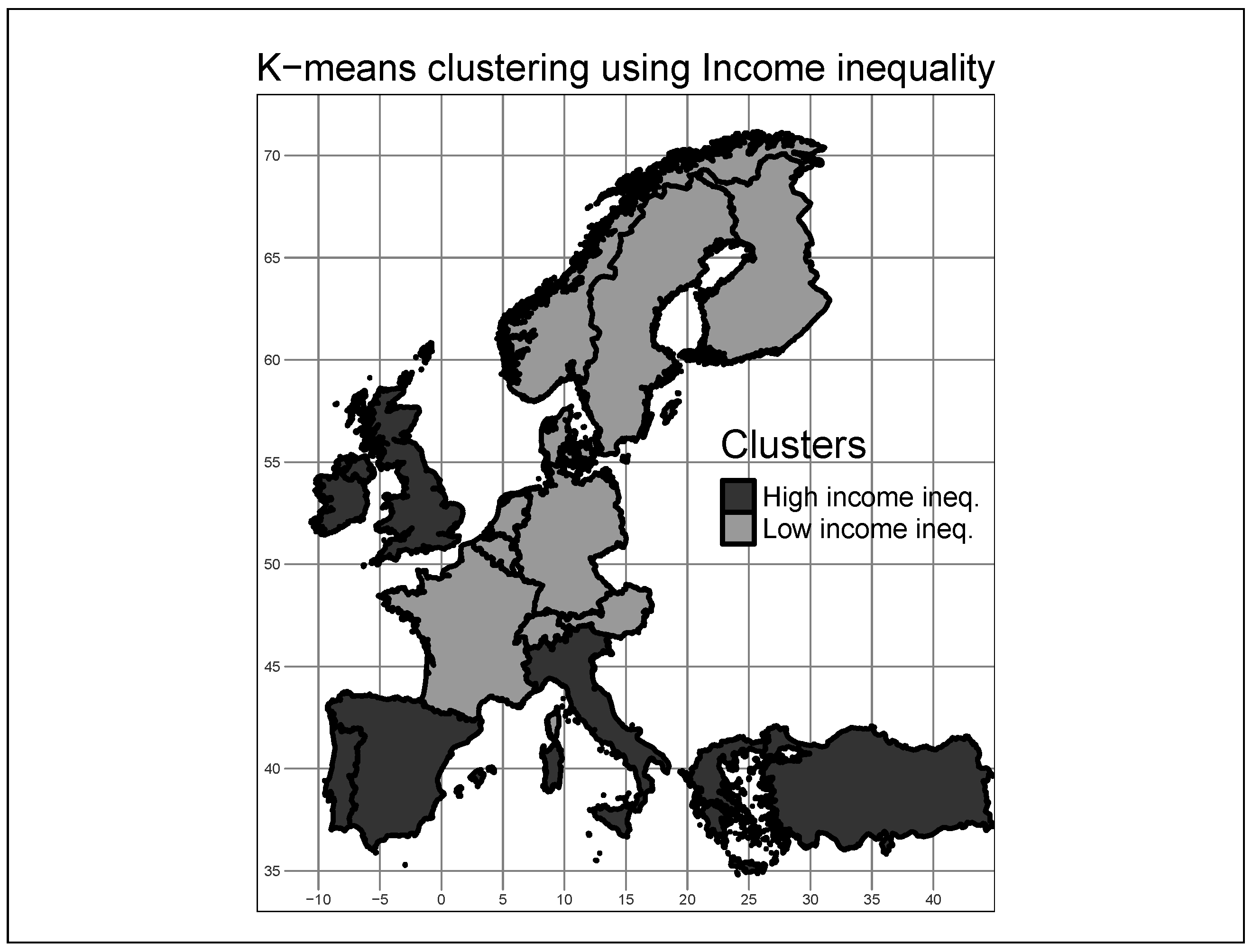
4.1. K-Means Clustering Using Income Inequality

As stated in Section 3.6, the use of income inequality measures in the EKC framework allows to properly identify the impact of economic variables on environmental quality and contributes to the debate on the role of income distribution [4]. For this reason, we use clustering analysis to gain some valuable insights into our data set by separating countries into groups according to their level of income inequality across the last decades. This study applies an innovative approach to country grouping based on the temporal evolution of income inequality and uses as clustering variables the annual values of the Gini Index on disposable income from 1987 to 2015. This approach partitions the countries according to their cross-sectional distances, obtaining groups of countries that share a “common evolutionary path” of income inequality. The use of socio-economic indicators to aggregate countries or regions and evaluate comparative performances has been considered in the literature. For example, the clustering of more than 150 countries based on Human Well-Being indicators of the Social Society Indices has been used [59,63], while composite indicators to generate a ranking of EU countries according to their sustainability in terms of lifestyle, environment, and social issues have also been calculated [64].
Cluster analysis techniques, such as K-means, are multivariate statistical methods used to obtain groups of observations based on their similarity to a set of specific features X. The K-means algorithm has the objective to partition n observations into k clusters, assigning each observation to the group with the nearest mean value and retaining the maximum inter-group and the minimum intra-group heterogeneity. The literature offers various examples of studies using clustering techniques based on inequality measures to classify countries [65]. Findings show structural differences between groups of countries in terms of social indicators, particularly about income inequality measures, with a reduced dynamicity from one group to another along time.
Our study seeks to classify the countries in the panel data set through the K-means algorithm using the information on income inequality, setting as grouping variables the yearly values of the Gini Index on disposable income from 1987 to 2015. Formally, the set of cluster features available for each country i = 1 , 2 , , 17 can be expressed as X i = X i , 1987 , X i , 1988 , , X i , t , , X i , 2014 , X i , 2015 , where t = 1987 , , 2015 and X i t represents the observed Gini Index for country i at time t.
Since we study the impact of the level of education on the environment–growth relationship by controlling for income inequality, we have decided to use the most straightforward classification strategy with K = 2 potential groups. Given the small number of cross-sectional units (17 countries), a clustering algorithm with a larger number of groups would harm the robustness of the panel regression analysis. In addition, from an interpretative perspective, this assumption allows identifying two distinguished groups of European OECD countries, characterized by common temporal patterns that can be traced back to historical events that occurred during the period 1950 to 2015.

4.2. Panel Data Analysis

All EKC models are tested using panel data techniques [66] with fixed-effects (FE) and random-effects (RE) model specifications. The FE model assumes that the individual effects are fixed parameters to be estimated and the disturbances are I.ID. with zero mean and constant variance. The RE specification allows the individual effects to be random and I.ID. distributed with zero mean and constant variance. FE and RE are compared using a Hausman’s specification test [67,68]. The software Stata 16 [69] is used to estimate the FE and RE specifications and to compute all the diagnostic tests, including cross-sectional dependence, unit-root, and cointegration. Data management, cluster analysis, and graphical analysis are performed using the software R [70].

5. Empirical Results

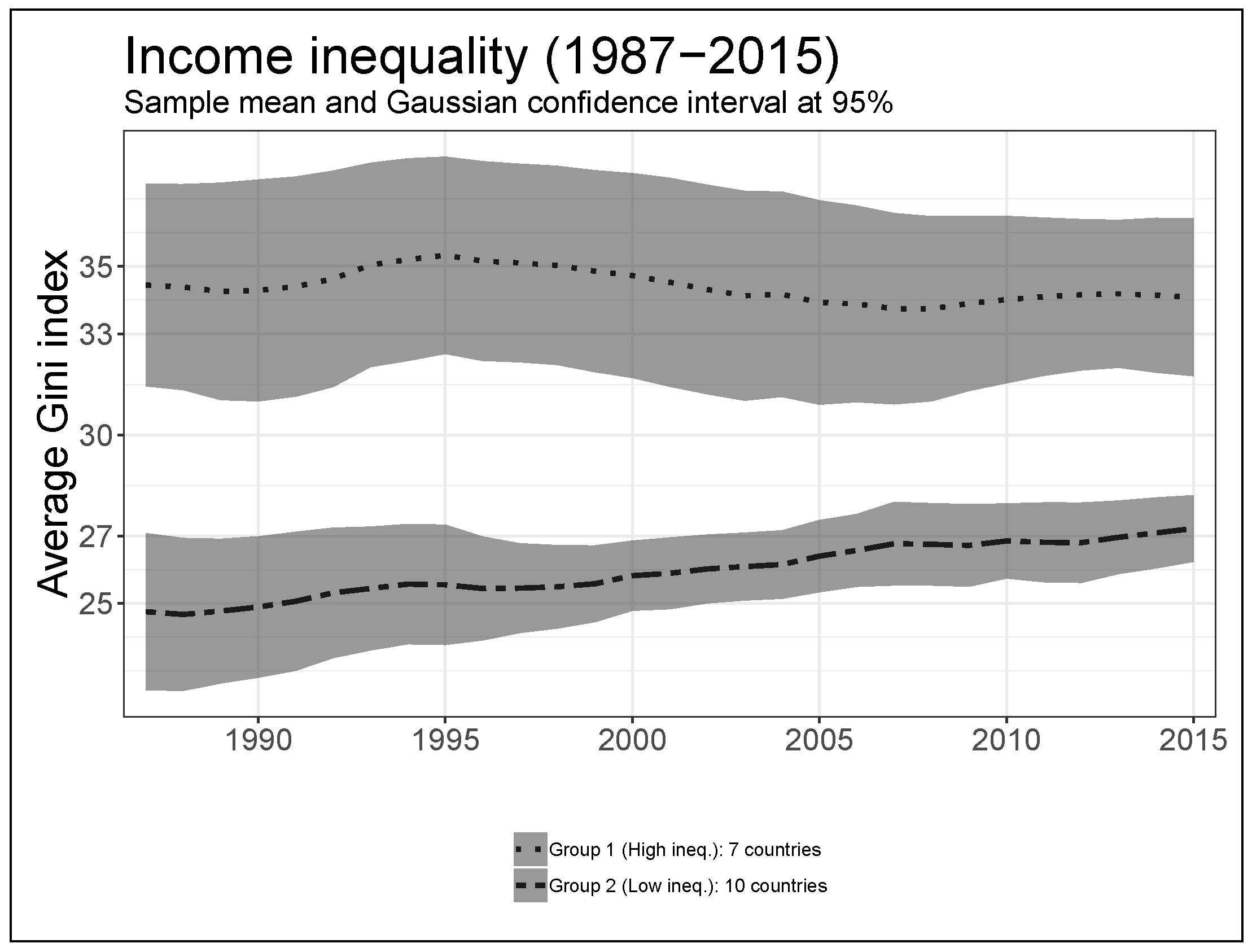
5.1. Cluster of the Income Inequality Trajectories

The K-means procedure identified two distinct groups of 7 and 10 countries, respectively. The smaller group is composed by countries that share a common high income inequality path with a decreasing trend, therefore appointed as ‘High income inequality cluster’. In comparison, the larger group is composed of countries with a generally lower income inequality with increasing perspectives, named ‘Low income inequality cluster’.
The high income inequality group (dark gray) includes Mediterranean countries, the United Kingdom, Ireland, and Turkey, while the low income inequality block (light gray) includes Central and Northern Europe economies. Table 2 reports the list of countries belonging to each group. Figure 2 shows the geographical partition of the selected countries among the two groups.
The two temporal patterns, represented in Figure 3, confirm previous expectations, namely, that OECD countries are strongly heterogeneous in terms of income distribution and run parallel paths that converge very slowly. Also, Figure 3 highlights two other crucial facts. The first is the remarkable increasing trend of income inequality for countries that initially had very low levels of the Gini Index. The second aspect is the convergence in terms of disparities among the two blocks. These results reflect both recent and historical events related to the development and growth of the area. Due to financial crises and general slowdowns of growth, in the last decades the distance among OECD countries in terms of income distribution and economic perspectives increased strongly and generated structural economic divergences as well as the rising of new social issues and demands about the growing inequalities. The strong growth of the low income inequality group and the consolidation of the high income inequity countries is symptomatic of an asymmetry in the long-term effects of these phenomena.

5.2. Panel Regression Analysis

5.2.1. Endogeneity Tests

The EKC literature has investigated endogeneity problems linking the environmental variables to many covariates. In this paper, we tested the hypothesis of endogeneity among the dependent variable and every regressor included in the models. In particular, endogeneity issues are related to the trade openness of countries and the amount of renewable energy consumption over the total. Intuitively, international trade exchanges are direct pollution sources due to logistics and transportation. However, there could be a reverse causality issue, since more polluting countries or regions may be less attractive for trading agreements and investments. In addition, energy production and consumption influence directly the amount of air pollution, according to their dual composition of sustainable and non-sustainable energy sources. Due to climate change and pollution excess, the growing legislation in defense of the environment has generated an innovative inverse causality-flow, which has increased the global demand for more sustainable and green energy sources and the exploitation of environment-friendly technologies.
To empirically test the endogeneity of the variables reported in Table 3, we performed the Davidson–Mackinnon test [71] by using as instrument for each variable its one-period lag. The Davidson–Mackinnon approach allows testing the null hypothesis of consistency of the OLS estimates for panel data against the alternative hypothesis that the OLS estimator is inconsistent and an instrumental variable technique is more appropriate. The rejection of the null hypothesis would suggest the presence of endogeneity of the considered regressors.
According to the results of the tests summarized in Table 3, the data do not provide enough statistical significance to reject the null hypothesis of exogeneity between the variables, except for energy use. Thus, to avoid inconsistency, instrumental variables estimation methods will be considered.
Hypothesis 0.
Exogenous regressor, alternative.
Hypothesis 1.
Endogenous regressor.

5.2.2. Unit Root and Cointegration Tests

Given the relevance of the time dimension in our panel, we analyze the stationarity and cointegration conditions of the system. Panel stationarity of each variable and its first difference transformation are investigated using the popular first-generation tests by Levin–Lin–Chu [72] and Im–Pesaran–Shin [73], with a time trend variable included. Empirical results of the panel stationary tests are available in Table 4 and Table 5.
Hypothesis 2.
All the panels contain unit roots.
Hypothesis 3.
Some panels are stationary.
Hypothesis 4.
Panels contain unit roots.
Hypothesis 5.
Panels are stationary.
Considering the log-levels, CO2 emissions, per capita income, education level, and energy use are non-stationary, but become stationary when considering their first differences. When a time trend is included in the analysis, both tests confirm that trade openness becomes stationary. While adding just a constant term, the tests do not reject the null hypothesis of unit-root in the panels. The overall picture becomes even more clouded if we use the CIPS test by Pesaran [74], which allows for cross-sectional dependence among different panel units (second-generation test). In this case, trade openness, energy use, and the square of per capita income are non-stationary, while for CO2 emissions, per capita income, education, and its square, the test does not indicate the presence of unit roots (Table 6).
Hypothesis 6.
Homogeneous non-stationary panels.
Hypothesis 7.
Stationary panels.
The variability in the performance of the most commonly used panel unit root tests is well-known in the literature [75]. Moreover, their limited adequacy when requested to deal with non-linear transformations of integrated variables, such as squares of per capita income, is acknowledged [16,75,76]. In the light of the mixed evidence provided by those tests and the major aim of this paper, which is to provide further empirical evidence on the economic aspects and implications of the EKC hypothesis, we proceed to the analysis of cointegration, implicitly assuming that the series are integrated of order one, i.e., I(1). We employed the panel cointegration tests proposed by Pedroni [77,78] and Westerlund [79,80]. The results of Pedroni and Westerlund panel cointegration tests are reported in Table 7, Table 8 and Table 9.
Hypothesis 8.
No cointegration.
Hypothesis 9.
Cointegrated panel.
Hypothesis 10.
No cointegration.
Hypothesis 11.
Cointegration between some of the cross-sectional units (some panels) or Cointegration between all cross-sectional units (all panels).
Hypothesis 12.
No cointegration.
Hypothesis 13.
Cointegration between at least one of the cross-sectional units (Gt and Ga) or Cointegration for panel as a whole (Pt and Pa).
The data do not provide strong statistical evidence of cointegration relationships between the variables. Specifically, all seven Pedroni statistics contradict each other, both at the group and panel level, showing observed values close to the critical ones, while the Westerlund tests suggest the absence of cointegration. While cointegration tests suffer from the same problems of the unit root statistics, especially when non-linear transformations of variables are present [76], nevertheless the Augmented Dickey–Fuller versions of Pedroni’s panel and group tests (tests four and seven in Table 7) exhibit a good performance in terms of size and power and are less severely affected by I(2) components and short-run cross-sectional correlation [81]. We have also included a dummy for capturing the structural breaks in the time series due to the 2008–2012 crisis. In this case, the previously cited tests provide minimal changes of p-values, without affecting our conclusions.

5.2.3. Estimates for the Full Sample

Both FE and RE models are estimated using the full sample from 1950 to 2015 and including energy use as an endogenous covariate. The estimation results are reported in Table 10.
Regarding the EKC model specification, both models provide statistically significant coefficients of per capita income and per capita income squared, and coherence of signs with respect to the expectations. Hence, the data lead to conclusions in favor of the EKC for the selected panel of OECD countries. Estimated turning points ( T P ) of per capita income for FE model and RE model are respectively T P F E = USD 64,320 per capita and T P R E = USD 55,157. Both values are included within the empirical range of the sample, strengthening the existence of the curve. Even the quadratic relationship between pollution and education is validated. All the related coefficients are statistically significant and respect the expected signs, leading to an inverted-U curve for increasing values of years of schooling. At the aggregate level, the educational turning points using FE and RE are calculated at 4.60 and 5.37 years of schooling, respectively. According to these results, it is possible to infer that data for the selected OECD countries support the empirical evidence of a Standard EKC and Educational EKC.
We recall that we calculated energy use as the ratio of renewable energy production over total energy production, given by the sum of both renewable and non-renewable productions of energy. Then, we expect that the estimated coefficient is negative, meaning that an increase in renewable energy production corresponds to a reduction in atmospheric emissions. In both FE and RE estimators, the impact of energy production on CO2 emissions is estimated with a negative sign and significant coefficients, consistent with expectations. In particular, both models suggest that a percentage increase in energy produced through renewable sources might reduce the CO2 emissions by 0.12 percentage points. On the contrary, data do not support statistically significant coefficients for trade openness, whose impact is estimated to be positive but close to zero. To identify the more appropriate model specification, we use the Hausman’s specification test, which compares the FE and RE estimators under the null hypothesis of uncorrelation between the regressors and error terms. The test statistic is equal to 64.25, providing enough statistical information to reject the null hypothesis and to conclude in favor of the FE estimator.

5.2.4. Estimates for the Grouped Samples

To reinforce the hypothesis of a significant effect of schooling on environmental degradation and to engage the social theme of wealth distribution, we developed a sensitivity analysis by re-estimating the panel regressions with fixed effects for each group identified using the clustering algorithm. As discussed above, the countries were divided into two clusters based on the temporal evolution of income inequality and characterized by widely different values of the Gini Index. Table 11 contains the FE estimates of the parameters for both groups of countries.
Compared to the overall sample, the two groups differ considerably and present interesting features. The EKC hypothesis holds only for high income inequality countries, while the coefficient associated with the quadratic income term is no more statistically significant in the complementary group. The Educational EKC hypothesis is validated for both clusters, but the educational turning point of the high income inequality group, i.e., T P E d u , H i g h = 1.002 , does not provide a meaningful economic interpretation. The estimates for both groups of countries show that energy production from renewable sources still plays a crucial role in mitigating airborne pollutant emissions. In both groups, its coefficient is negative and statistically significant. In fact, the estimate of the coefficient of energy use for countries with low income inequality is smaller than in the full sample, moving from −0.12 to −0.09 (a 1% increase in renewable production is associated with a reduction in CO2 emissions of 0.09%), while for countries with greater levels of inequality the coefficient increases in absolute value to 0.13 (a 1% increase in renewable production is associated with a reduction in CO2 emissions of 0.13%).
Moreover, trade openness becomes significant, and for each percentage of trade openness, low income inequality countries enjoy a reduction in emissions of 0.125%, hence validating the pollution haven hypothesis. On the contrary, high income inequality countries suffer from the opposite effect, namely, a 1% increase in international trade is associates with a 0.145% increase in CO2 emissions, supporting the pollution halo hypothesis. According to these results, the clustering highlighted the presence of different effects of economic development and human capital on environmental quality differentiated by levels of income inequality within the countries.

6. Discussion

The lack of empirical verification of the EKC hypothesis for the set of countries with low levels of inequality and the simultaneous validation of the Educational EKC hypothesis deserve to be further investigated and open a debate on new adoptable functional forms. Moreover, some of those countries represent in empirical studies positive examples for the EKC theory [22,82,83]. The role of education in long-run development is crucial. Investments in strengthening educational systems and facilities, supported by other structural reforms of the labor market, companies, and taxation, can push growth and at the same time reduce the level of social inequality [84]. Countries with low income inequality show a very strong positive linear correlation between GDP and average years of schooling, greater than that observed in countries with higher inequality. Table 12 and Table 13 provide the Pearson’s correlation coefficients between per capita income, education, and pollution levels grouped by cluster.
In those countries where the level of income inequality is lower, the link between educational level and personal income, measured by their positive linear correlation, seems to be very strong and steady. This empirical evidence is consistent with many studies in the field of development economics that identify schooling and education as determinants of personal income and capital endowment of a country and, therefore, promoters of higher economic growth [32,85]. Furthermore, the linear correlation between per capita income and level of pollutants is very close to the linear correlation between education and pollutants. Both are very low and are symptoms of a non-linear relationship between the variables.
Given these facts, we propose a different specification of the EKC that employs the educational variable, i.e., years of schooling, as the primary driver of environmental degradation instead of personal income. From an econometric perspective, the simultaneous presence of average years of schooling and per capita income among the set of regressors could imply severe multicollinearity issues and generate inconsistent estimates. The new specification is applied to countries with high income inequality and countries with low income inequality. The specification which uses the years of schooling as a regressor is called Educational EKC, while the one with the level of income per capita remains the Standard EKC. For each group, the estimate of the Educational EKC is compared with the Standard EKC specification. Estimates for the alternative EKC specification are available in Table 14, which reports the estimated coefficients for the four models.
Considering low income inequality countries, renewable energy use and trade openness have negative signs and similar values in the models, i.e., an increase in renewable energy share of one percent can generate a reduction around 0.086% in pollution (CO2) levels. In addition, international trade plays a role in emissions reduction: a percentage point increase in trade openness corresponds to a reduction of pollution levels between 0.1% and 0.3%. The estimated turning points for the two models are T P L o w , G D P = 85.523$ and T P L o w , E d u = 10.83 years, respectively. None of the low income inequality countries reached the monetary turning point. The country with greater personal income is Norway, which registered a value of 84,417$ in 2007. On the contrary, the educational turning point is achieved by low income inequality countries: Switzerland (1967), Germany (1978), Norway (1985), Sweden (1989), Denmark (1990), Netherlands (1998), Finland (1999), Austria (2000), Belgium (2012), and France (2013). This fact confirms the robustness of the Educational EKC specification with respect the Standard EKC with quadratic terms. In Figure 4, we represent the observed relationship between years of schooling and CO2 per capita (Educational EKC, left panel) and between income per capita and CO2 per capita (Standard EKC, right panel) for low income inequality countries.
Independently from the cluster, all the estimated coefficients are statistically significant and have the expected signs. The Standard EKC and the Educational EKC are validated in the two samples.
In addition, as shown by the country-by-country plots provided in Appendix A, some countries properly match the inverted-U shape form of the EKC because they follow the same behavior of the aggregate EKC model closely, and other countries exhibit less similarities with the theoretical EKC pattern. In particular, both Educational EKC and Standard EKC specifications are better performing for the cluster of low income inequality countries. We infer from the graphs that low income inequality countries are more advanced economies and dispose of a large amount of resources to invest into environment-friendly technologies, accelerating the decarbonization process towards a cleaner production, which is less harmful to the environment.

7. Conclusions

The present paper has assessed the relationship between the role of education and income inequality on environmental quality using a panel data approach for 17 selected OECD and European countries, by taking into account the historical evolution of their income inequality pathways. The clustering analysis based on the Gini Index has highlighted structural differences in the paths of the sampled countries. The statistical approach has generated heterogeneous income inequality patterns and has led to different growth impacts on the natural environment. In addition, the variable modeling the role of education has been embedded in the models by augmenting the Standard EKC specification with a quadratic term for the average years of schooling. The research findings indicate clear results for the cluster of low income inequality countries and plausible turning points.
We have employed panel data models which provided statistically significant and acceptable estimates of the parameters, suggesting the existence of an inverted-U EKC curve both for the Standard and Educational specifications. The Educational EKC has underlined the non-linearity in the relationship between education and emissions, reflecting the dynamic change in economic and social development. Moreover, this study is not only grounded on statistical methods. Our findings have mainly highlighted the economic aspects and implications of the EKC research design. For this reason, we argue that the type of research methodology makes use of verifiable evidence in order to arrive at research outcomes. In fact, we have provided further evidence on the relationship between education and the environment which has been supported within the EKC framework.
We encourage researchers to replace the Standard EKC with an educational-based specification, namely, the Educational EKC. Further research should consider the level of schooling and inequality of countries as the main drivers of socio-economic development, along with other relevant variables and pollutant emissions, in the EKC framework.

Author Contributions

Conceptualization, P.M., J.P.C.B. and M.M.; methodology, P.M., J.P.C.B. and M.M.; software, P.M.; validation, P.M., J.P.C.B. and M.M.; formal analysis, P.M., J.P.C.B. and M.M.; investigation, P.M.; resources, P.M.; data curation, P.M.; writing—original draft preparation, P.M.; writing—review and editing, P.M., J.P.C.B. and M.M.; visualization, P.M., J.P.C.B. and M.M.; supervision, J.P.C.B. and M.M.; project administration, P.M. All authors have read and agreed to the published version of the manuscript.

Funding

This research received no external funding.

Institutional Review Board Statement

Not applicable.

Informed Consent Statement

Not applicable.

Data Availability Statement

Data and codes can be requested by email to Paolo Maranzano ([email protected]).

Conflicts of Interest

The authors declare no conflict of interest.

Abbreviations

The following abbreviations are used in this manuscript:
EKCEnvironmental Kuznets Curve
Edu_EKCEducational Environmental Kuznets Curve
TPTurning point
PWTPenn World Tables
FEFixed-effects model
RERandom-effects model

Appendix A. Environmental and Educational EKC by Countries and Income Inequality Level

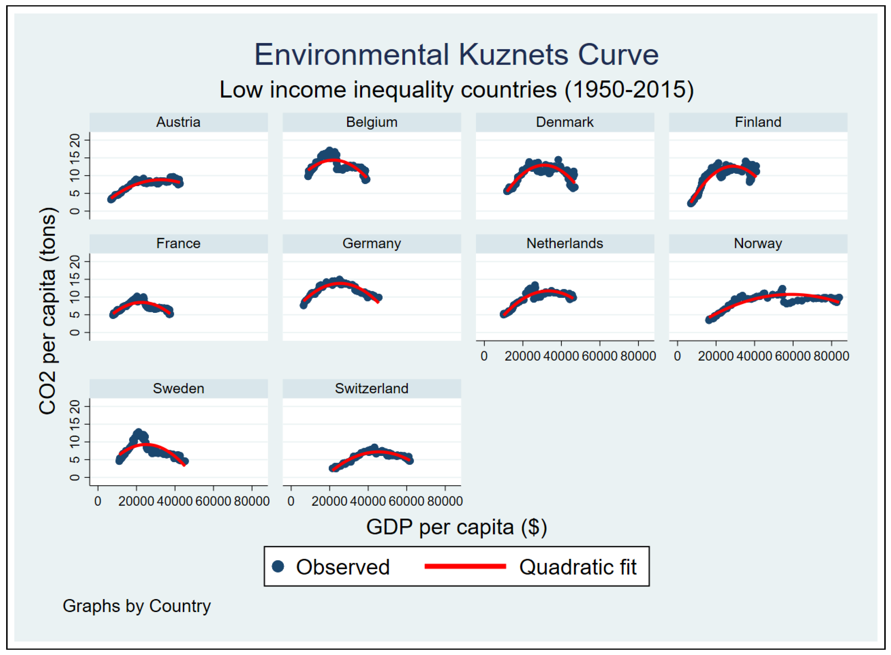
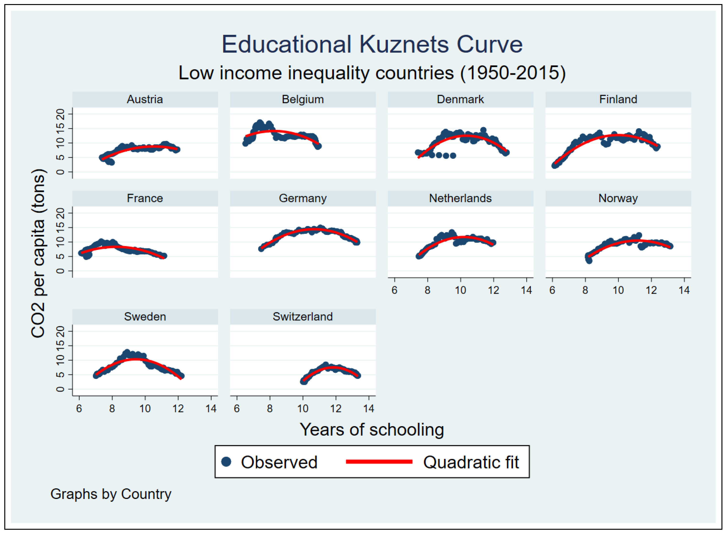
Appendix A.1. Low Income Inequality Countries

Figure A1. Educational Kuznets Curve for low income inequality countries. Blue points are the observed values, red curves are the quadratic fit for each country. Own elaboration based on our estimation results.
Sustainability 14 01622 g0a1
Figure A2. Environmental Kuznets Curve for low income inequality countries. Blue points are the observed values, red curves are the quadratic fit for each country. Own elaboration based on our estimation results.
Sustainability 14 01622 g0a2

Appendix A.2. High Income Inequality Countries

Figure A3. Educational Kuznets Curve for high income inequality countries. Blue points are the observed values, red curves are the quadratic fit for each country. Own elaboration based on our estimation results.
Sustainability 14 01622 g0a3
Figure A4. Environmental Kuznets Curve for high income inequality countries. Blue points are the observed values, red curves are the quadratic fit for each country. Own elaboration based on our estimation results.
Sustainability 14 01622 g0a4

References

  1. Grossman, G.M.; Krueger, A.B. Environmental Impacts of a North American Free Trade Agreement; Technical Report; National Bureau of Economic Research: Cambridge, MA, USA, 1991. [Google Scholar]
  2. Stern, D.I. The environmental Kuznets curve after 25 years. J. Bioecon. 2017, 19, 7–28. [Google Scholar] [CrossRef] [Green Version]
  3. Balaguer, J.; Cantavella, M. The role of education in the Environmental Kuznets Curve. Evidence from Australian data. Energy Econ. 2018, 70, 289–296. [Google Scholar] [CrossRef]
  4. Sapkota, P.; Bastola, U. Foreign direct investment, income, and environmental pollution in developing countries: Panel data analysis of Latin America. Energy Econ. 2017, 64, 206–212. [Google Scholar] [CrossRef]
  5. Kuznets, S. Economic Growth and Income Inequality. Am. Econ. Rev. 1955, 45, 1–28. [Google Scholar]
  6. Grossman, G.M.; Krueger, A.B. Economic Growth and the Environment*. Q. J. Econ. 1995, 110, 353–377. [Google Scholar] [CrossRef] [Green Version]
  7. Cerdeira Bento, J.P.; Moutinho, V. CO2 emissions, non-renewable and renewable electricity production, economic growth, and international trade in Italy. Renew. Sustain. Energy Rev. 2016, 55, 142–155. [Google Scholar] [CrossRef]
  8. Alvarez-Herranz, A.; Balsalobre-Lorente, D.; Shahbaz, M.; Cantos, J.M. Energy innovation and renewable energy consumption in the correction of air pollution levels. Energy Policy 2017, 105, 386–397. [Google Scholar] [CrossRef]
  9. Coondoo, D.; Dinda, S. Causality between income and emission: A country group-specific econometric analysis. Ecol. Econ. 2002, 40, 351–367. [Google Scholar] [CrossRef]
  10. Stern, D.I. The rise and fall of the environmental Kuznets curve. World Dev. 2004, 32, 1419–1439. [Google Scholar] [CrossRef]
  11. Stern, D.I. Progress on the environmental Kuznets curve? Environ. Dev. Econ. 2001, 3, 173–196. [Google Scholar] [CrossRef]
  12. Gill, A.R.; Viswanathan, K.K.; Hassan, S. A test of environmental Kuznets curve (EKC) for carbon emission and potential of renewable energy to reduce green house gases (GHG) in Malaysia. Environ. Dev. Sustain. 2018, 20, 1103–1114. [Google Scholar] [CrossRef]
  13. Dinda, S. Environmental Kuznets curve hypothesis: A survey. Ecol. Econ. 2004, 49, 431–455. [Google Scholar] [CrossRef] [Green Version]
  14. Ekins, P. Economic Growth and Environmental Sustainability: The Prospects for Green Growth; Routledge: London, UK, 2002. [Google Scholar]
  15. Wagner, M. The carbon Kuznets curve: A cloudy picture emitted by bad econometrics? Resour. Energy Econ. 2008, 30, 388–408. [Google Scholar] [CrossRef] [Green Version]
  16. Müller-Fürstenberger, G.; Wagner, M. Exploring the environmental Kuznets hypothesis: Theoretical and econometric problems. Ecol. Econ. 2007, 62, 648–660. [Google Scholar] [CrossRef] [Green Version]
  17. Hasanov, F.J.; Hunt, L.C.; Mikayilov, J.I. Estimating different order polynomial logarithmic environmental Kuznets curves. Environ. Sci. Pollut. Res. 2021, 28, 41965–41987. [Google Scholar] [CrossRef] [PubMed]
  18. Feenstra, R.C.; Inklaar, R.; Timmer, M.P. The next generation of the Penn World Table. Am. Econ. Rev. 2015, 105, 3150–3182. [Google Scholar] [CrossRef] [Green Version]
  19. Solt, F. The standardized world income inequality database. Soc. Sci. Q. 2016, 97, 1267–1281. [Google Scholar] [CrossRef]
  20. Rasli, A.M.; Qureshi, M.I.; Isah-Chikaji, A.; Zaman, K.; Ahmad, M. New toxics, race to the bottom and revised environmental Kuznets curve: The case of local and global pollutants. Renew. Sustain. Energy Rev. 2018, 81, 3120–3130. [Google Scholar] [CrossRef]
  21. Al-Mulali, U.; Weng-Wai, C.; Sheau-Ting, L.; Mohammed, A.H. Investigating the environmental Kuznets curve (EKC) hypothesis by utilizing the ecological footprint as an indicator of environmental degradation. Ecol. Indic. 2015, 48, 315–323. [Google Scholar] [CrossRef]
  22. Iwata, H.; Okada, K.; Samreth, S. Empirical study on the determinants of CO2 emissions: Evidence from OECD countries. Appl. Econ. 2012, 44, 3513–3519. [Google Scholar] [CrossRef] [Green Version]
  23. Saboori, B.; Sulaiman, J. Environmental degradation, economic growth and energy consumption: Evidence of the environmental Kuznets curve in Malaysia. Energy Policy 2013, 60, 892–905. [Google Scholar] [CrossRef]
  24. Galeotti, M.; Manera, M.; Lanza, A. On the Robustness of Robustness Checks of the Environmental Kuznets Curve Hypothesis. Environ. Resour. Econ. 2008, 42, 551. [Google Scholar] [CrossRef]
  25. Beck, K.A.; Joshi, P. An analysis of the environmental Kuznets curve for carbon dioxide emissions: Evidence for OECD and Non-OECD countries. Eur. J. Sustain. Dev. 2015, 4, 33. [Google Scholar]
  26. Churchill, S.A.; Inekwe, J.; Ivanovski, K.; Smyth, R. The environmental Kuznets curve in the OECD: 1870–2014. Energy Econ. 2018, 75, 389–399. [Google Scholar] [CrossRef]
  27. Leal, P.H.; Marques, A.C. Rediscovering the EKC hypothesis for the 20 highest CO2 emitters among OECD countries by level of globalization. Int. Econ. 2020, 167, 36–47. [Google Scholar] [CrossRef]
  28. Ehrhardt-Martinez, K.; Crenshaw, E.M.; Jenkins, J.C. Deforestation and the environmental Kuznets curve: A cross-national investigation of intervening mechanisms. Soc. Sci. Q. 2002, 83, 226–243. [Google Scholar] [CrossRef]
  29. Magnani, E. The Environmental Kuznets Curve, environmental protection policy and income distribution. Ecol. Econ. 2000, 32, 431–443. [Google Scholar] [CrossRef]
  30. Sala-i Martin, X.X.; Barro, R.J. Technological Diffusion, Convergence, and Growth; Report, Center Discussion Paper; Center Discussion Paper No. 735; Yale University, Economic Growth Center: New Haven, CT, USA, 1995. [Google Scholar]
  31. Barro, R.J. Human Capital and Growth in Cross-Country Regressions. Ph.D. Thesis, Harvard University, Cambridge, MA, USA, 1998. [Google Scholar]
  32. Barro, R.J. Human capital and growth. Am. Econ. Rev. 2001, 91, 12–17. [Google Scholar] [CrossRef]
  33. Benhabib, J.; Spiegel, M.M. The role of human capital in economic development evidence from aggregate cross-country data. J. Monet. Econ. 1994, 34, 143–173. [Google Scholar] [CrossRef]
  34. Gundlach, E. The role of human capital in economic growth: New results and alternative interpretations. Weltwirtschaftliches Arch. 1995, 131, 383–402. [Google Scholar] [CrossRef] [Green Version]
  35. Islam, N. Growth Empirics: A Panel Data Approach*. Q. J. Econ. 1995, 110, 1127–1170. [Google Scholar] [CrossRef]
  36. Krueger, A.B.; Lindahl, M. Education for growth: Why and for whom? J. Econ. Lit. 2001, 39, 1101–1136. [Google Scholar] [CrossRef] [Green Version]
  37. O’neill, D. Education and income growth: Implications for cross-country inequality. J. Political Econ. 1995, 103, 1289–1301. [Google Scholar] [CrossRef] [Green Version]
  38. Temple, J.R. Generalizations that aren’t? Evidence on education and growth. Eur. Econ. Rev. 2001, 45, 905–918. [Google Scholar] [CrossRef]
  39. Pata, U.K. Renewable energy consumption, urbanization, financial development, income and CO2 emissions in Turkey: Testing EKC hypothesis with structural breaks. J. Clean. Prod. 2018, 187, 770–779. [Google Scholar] [CrossRef]
  40. Zhang, B.; Wang, B.; Wang, Z. Role of renewable energy and non-renewable energy consumption on EKC: Evidence from Pakistan. J. Clean. Prod. 2017, 156, 855–864. [Google Scholar] [CrossRef]
  41. Usman, O.; Iorember, P.T.; Olanipekun, I.O. Revisiting the environmental Kuznets curve (EKC) hypothesis in India: The effects of energy consumption and democracy. Environ. Sci. Pollut. Res. 2019, 26, 13390–13400. [Google Scholar] [CrossRef]
  42. Shahbaz, M.; Mutascu, M.; Azim, P. Environmental Kuznets curve in Romania and the role of energy consumption. Renew. Sustain. Energy Rev. 2013, 18, 165–173. [Google Scholar] [CrossRef] [Green Version]
  43. Dogan, E.; Turkekul, B. CO2 emissions, real output, energy consumption, trade, urbanization and financial development: Testing the EKC hypothesis for the USA. Environ. Sci. Pollut. Res. 2016, 23, 1203–1213. [Google Scholar] [CrossRef]
  44. Jaforullah, M.; King, A. The econometric consequences of an energy consumption variable in a model of CO2 emissions. Energy Econ. 2017, 63, 84–91. [Google Scholar] [CrossRef]
  45. Ang, J.B. CO2 emissions, energy consumption, and output in France. Energy Policy 2007, 35, 4772–4778. [Google Scholar] [CrossRef]
  46. Apergis, N.; Payne, J.E. Renewable Energy, Output, Carbon Dioxide Emissions, and Oil Prices: Evidence from South America. Energy Sources Part Econ. Plan. Policy 2015, 10, 281–287. [Google Scholar] [CrossRef]
  47. Dogan, E.; Seker, F. Determinants of CO2 emissions in the European Union: The role of renewable and non-renewable energy. Renew. Energy 2016, 94, 429–439. [Google Scholar] [CrossRef]
  48. Zambrano-Monserrate, M.A.; Silva-Zambrano, C.A.; Davalos-Penafiel, J.L.; Zambrano-Monserrate, A.; Ruano, M.A. Testing environmental Kuznets curve hypothesis in Peru: The role of renewable electricity, petroleum and dry natural gas. Renew. Sustain. Energy Rev. 2018, 82, 4170–4178. [Google Scholar] [CrossRef]
  49. Esmaeili, A.; Abdollahzadeh, N. Oil exploitation and the environmental Kuznets curve. Energy Policy 2009, 37, 371–374. [Google Scholar] [CrossRef]
  50. Burnett, J.W.; Bergstrom, J.C.; Wetzstein, M.E. Carbon dioxide emissions and economic growth in the U.S. J. Policy Model. 2013, 35, 1014–1028. [Google Scholar] [CrossRef]
  51. Itkonen, J.V. Problems estimating the carbon Kuznets curve. Energy 2012, 39, 274–280. [Google Scholar] [CrossRef]
  52. Jebli, M.B.; Youssef, S.B.; Ozturk, I. Testing environmental Kuznets curve hypothesis: The role of renewable and non-renewable energy consumption and trade in OECD countries. Ecol. Indic. 2016, 60, 824–831. [Google Scholar] [CrossRef]
  53. Acemoglu, D.; Autor, D. What Does Human Capital Do? A Review of Goldin and Katz’s The Race between Education and Technology. J. Econ. Lit. 2012, 50, 426–463. [Google Scholar] [CrossRef] [Green Version]
  54. Acemoglu, D.; Gallego, F.A.; Robinson, J.A. Institutions, Human Capital, and Development. Annu. Rev. Econ. 2014, 6, 875–912. [Google Scholar] [CrossRef] [Green Version]
  55. Atkinson, A.B. On the measurement of inequality. J. Econ. Theory 1970, 2, 244–263. [Google Scholar] [CrossRef]
  56. De Maio, F.G. Income inequality measures. J. Epidemiol. Community Health 2007, 61, 849–852. [Google Scholar] [CrossRef] [PubMed]
  57. Gini, C. Measurement of inequality of incomes. Econ. J. 1921, 31, 124–126. [Google Scholar] [CrossRef]
  58. Pontusson, J.; Weisstanner, D. Macroeconomic conditions, inequality shocks and the politics of redistribution, 1990–2013. J. Eur. Public Policy 2018, 25, 31–58. [Google Scholar] [CrossRef]
  59. Hao, Y.; Chen, H.; Zhang, Q. Will income inequality affect environmental quality? Analysis based on China’s provincial panel data. Ecol. Indic. 2016, 67, 533–542. [Google Scholar] [CrossRef]
  60. Heerink, N.; Mulatu, A.; Bulte, E. Income inequality and the environment: Aggregation bias in environmental Kuznets curves. Ecol. Econ. 2001, 38, 359–367. [Google Scholar] [CrossRef]
  61. Ridzuan, S. Inequality and the environmental Kuznets curve. J. Clean. Prod. 2019, 228, 1472–1481. [Google Scholar] [CrossRef]
  62. Vona, F.; Patriarca, F. Income inequality and the development of environmental technologies. Ecol. Econ. 2011, 70, 2201–2213. [Google Scholar] [CrossRef]
  63. Akan, M.O.A.; Selam, A.A. Assessment of social sustainability using Social Society Index: A clustering application. Eur. J. Sustain. Dev. 2018, 7, 412–424. [Google Scholar] [CrossRef] [Green Version]
  64. Luzzati, T.; Gucciardi, G. A non-simplistic approach to composite indicators and rankings: An illustration by comparing the sustainability of the EU Countries. Ecol. Econ. 2015, 113, 25–38. [Google Scholar] [CrossRef]
  65. Neri, L.; D’Agostino, A.; Regoli, A.; Pulselli, F.M.; Coscieme, L. Evaluating dynamics of national economies through cluster analysis within the input-state-output sustainability framework. Ecol. Indic. 2017, 72, 77–90. [Google Scholar] [CrossRef]
  66. Baltagi, B. Econometric Analysis of Panel Data; John Wiley & Sons: New York, NY, USA, 2008. [Google Scholar]
  67. Hausman, J.A. Specification tests in econometrics. Econom. J. Econom. Soc. 1978, 46, 1251–1271. [Google Scholar] [CrossRef] [Green Version]
  68. Hausman, J.A.; Taylor, W.E. A generalized specification test. Econ. Lett. 1981, 8, 239–245. [Google Scholar] [CrossRef]
  69. StataCorp. Stata Release 16; StataCorp: College Station, TX, USA, 2017. [Google Scholar]
  70. R Core Team. R: A Language and Environment for Statistical Computing; R Foundation for Statistical Computing: Vienna, Austria, 2020. [Google Scholar]
  71. Davidson, R.; MacKinnon, J.G. Estimation and Inference in Econometrics; Oxford University Press: Oxford, UK, 1993. [Google Scholar]
  72. Levin, A.; Lin, C.F.; Chu, C.S.J. Unit root tests in panel data: Asymptotic and finite-sample properties. J. Econom. 2002, 108, 1–24. [Google Scholar] [CrossRef]
  73. Im, K.S.; Pesaran, M.H.; Shin, Y. Testing for unit roots in heterogeneous panels. J. Econom. 2003, 115, 53–74. [Google Scholar] [CrossRef]
  74. Pesaran, M.H. A simple panel unit root test in the presence of cross-section dependence. J. Appl. Econom. 2007, 22, 265–312. [Google Scholar] [CrossRef] [Green Version]
  75. Hlouskova, J.; Wagner, M. The Performance of Panel Unit Root and Stationarity Tests: Results from a Large Scale Simulation Study. Econom. Rev. 2006, 25, 85–116. [Google Scholar] [CrossRef] [Green Version]
  76. Hong, S.H.; Wagner, M. Nonlinear Cointegration Analysis and the Environmental Kuznets Curve; Report; Institute for Advanced Studies (IHS): Vienna, Austria, 2008. [Google Scholar]
  77. Pedroni, P. Critical values for cointegration tests in heterogeneous panels with multiple regressors. Oxf. Bull. Econ. Stat. 1999, 61, 653–670. [Google Scholar] [CrossRef]
  78. Pedroni, P. Purchasing power parity tests in cointegrated panels. Rev. Econ. Stat. 2001, 83, 727–731. [Google Scholar] [CrossRef] [Green Version]
  79. Westerlund, J. New simple tests for panel cointegration. Econom. Rev. 2005, 24, 297–316. [Google Scholar] [CrossRef]
  80. Westerlund, J. Testing for error correction in panel data. Oxf. Bull. Econ. Stat. 2007, 69, 709–748. [Google Scholar] [CrossRef] [Green Version]
  81. Wagner, M.; Hlouskova, J. The Performance of Panel Cointegration Methods: Results from a Large Scale Simulation Study. Econom. Rev. 2009, 29, 182–223. [Google Scholar] [CrossRef]
  82. Acaravci, A.; Ozturk, I. On the relationship between energy consumption, CO2 emissions and economic growth in Europe. Energy 2010, 35, 5412–5420. [Google Scholar] [CrossRef]
  83. Al-Mulali, U.; Ozturk, I. The investigation of environmental Kuznets curve hypothesis in the advanced economies: The role of energy prices. Renew. Sustain. Energy Rev. 2016, 54, 1622–1631. [Google Scholar] [CrossRef]
  84. Stiglitz, J.E. Inequality and economic growth. In Rethinking Capitalism; Wiley-Blackwell: Hoboken, NJ, USA, 2016; pp. 134–155. [Google Scholar]
  85. Castelló, A.; Doménech, R. Human capital inequality and economic growth: Some new evidence. Econ. J. 2002, 112, C187–C200. [Google Scholar] [CrossRef]
Figure 1. Income inequality trend in the OECD sample (1987–2015). The solid black line represents the sample mean of Gini Index on disposable income by year and the gray area is the approximate Gaussian confidence interval at 95% for the sample mean. Values are expressed in percentage.
Sustainability 14 01622 g001
Figure 2. Map of the clusters for the sample OECD countries. Dark gray countries belong to the ‘High income-inequality’ cluster and the light gray countries belong to the ‘Low income-inequality’ cluster.
Sustainability 14 01622 g002
Figure 3. Income inequality trend in the two clusters (1987–2015). The dotted black line represents the average annual Gini Index observed in the first sub-sample (‘High income-inequality’) and the dot-dashed black line represents the average annual Gini index for the second sub-sample (‘Low income-inequality’). Gray areas are the approximate Gaussian confidence interval at 95% for the sample mean. Values are expressed in percentage.
Sustainability 14 01622 g003
Figure 4. Environmental Kuznets Curve and Educational Kuznets Curve for low income inequality countries (panel fixed-effects estimator). Educational Kuznets Curve for low income inequality countries fitted using FE panel estimator (left panel) and Environmental Kuznets Curve for low income inequality countries fitted using FE panel estimator (right panel).
Sustainability 14 01622 g004
Table 1. Descriptive statistics for the considered variables.
Variable NameMeasure UnitMeanStd.Dev.MinMax
CO2 per capitaCO2 emissions
(metric tons per capita)
7.9555.420.4641.04
Income per capitaGDP per capita
(constant 2011 US$)
24,912.4614,390.293375.5084,417.24
EducationAverage years of schooling
(population 15–64 years)
8.612.740.9813.55
Energy useRenewable energy production over
total energy production
(percentage)
26%29%0%99%
Trade opennessSum of imports and
exports over GDP
(percentage)
65%47%1%286%
Table 2. K-means cluster results: countries by group.
ClusterMember Countries
Low income-inequality
(10 countries)
Austria, Belgium, Denmark, Finland, France, Germany
Netherlands, Norway, Sweden, and Switzerland
High income-inequality
(7 countries)
Greece, Ireland, Italy, Portugal
Spain, Turkey, and UK
Table 3. Exogeneity test (Davidson–Mackinnon) for each variable.
Variable NameF-Statisticp-Value
Income per capita2.4740.116
Income per capita squared2.4110.121
Education3.6640.056
Education squared0.0160.898
Energy use7.3200.007
Trade openness0.3090.579
Table 4. Im–Pesaran–Shin (2003) panel unit root test results.
Variable NameStatisticp-ValueDecision
CO2 per capita2.1360.984Non-stationary
Δ CO2 per capita−22.1130.000Stationary
Income per capita3.9100.999Non-stationary
Δ Income per capita−17.3380.000Stationary
Income per capita squared3.8480.999Non-stationary
Δ Income per capita squared−17.6270.000Stationary
Education3.9490.999Non-stationary
Δ Education−3.36630.000Stationary
Education squared−1.63540.0510Non-stationary
Δ Education squared−3.08350.001Stationary
Energy use−0.4870.313Non-stationary
Δ Energy use−22.0760.000Stationary
Trade openness1.15340.8756Stationary
Δ Trade openness−23.3280.000Stationary
Note. All variables are log-transformed. Trend is included. Lag lengths are selected by Akaike Information Criterion (AIC).
Table 5. Levin–Lin–Chu (2002) panel unit root test results.
Variable NameStatisticp-ValueDecision
CO2 per capita−0.44000.3300Non-stationary
Δ CO2 per capita−17.36160.000Stationary
Income per capita0.04190.5167Non-stationary
Δ Income per capita−16.09180.000Stationary
Income per capita squared0.84330.8005Non-stationary
Δ Income per capita squared−16.01730.000Stationary
Education0.20320.581Non-stationary
Δ Education−3.57000.000Stationary
Education squared−1.54790.0608Non-stationary
Δ Education squared−3.18640.000Stationary
Energy use0.21290.5843Non-stationary
Δ Energy use−18.9340.000Stationary
Trade openness0.27200.607Stationary
Δ Trade openness−21.6690.000Stationary
Note. All variables are log-transformed. Trend is included. Lag lengths are selected by Akaike Information Criterion (AIC).
Table 6. Pesaran’s CIPS panel unit root test (2007) in the presence of cross-section dependence.
Variable NameStatisticp-ValueDecision
CO2 per capita−2.865<0.01Stationary
Δ CO2 per capita−6.420<0.01Stationary
Income per capita−2.595<0.05Stationary
Δ Income per capita−5.872<0.01Stationary
Income per capita squared−2.508>0.10Non-stationary
Δ Income per capita squared−5.768<0.01Stationary
Education−3.534<0.01Stationary
Δ Education−2.410>0.10Non-stationary
Education squared−3.417<0.01Stationary
Δ Education squared−2.546>0.10Non-stationary
Energy use−2.199>0.10Non-stationary
Δ Energy use−5.584<0.01Stationary
Trade openness−2.545<0.10Non-stationary
Δ Trade openness−5.941<0.01Stationary
Note. All variables are log-transformed. Constant and trend are included. Lag lengths are selected by Akaike Information Criterion (AIC).
Table 7. Pedroni (1999) panel cointegration test results.
StatisticValuep-ValueDecision
Panel non par. v (VR)−0.93270.1755No cointegration
Panel non par. ρ (PP)−2.95290.0016Cointegration
Panel non par. t (PP)−6.88280.0000Cointegration
Panel par. t (ADF)−4.35490.0000Cointegration
Group non par. ρ (PP)−2.00610.0224Cointegration
Group non par. t (PP)−6.79380.0000Cointegration
Group par. t (ADF)−4.52350.0000Cointegration
Note. Constant and trend are included. The test is performed using all the variables, including the quadratic terms of per capita GDP and years of schooling (in total 7 variables). Lag lengths are selected by Akaike Information Criterion (AIC). Cross-sectional means removed.
Table 8. Westerlund (2005) variance-ratio cointegration test results, including quadratic terms.
StatisticValuep-ValueDecision
VR (some panels)−2.48110.0065Cointegration
VR (all panels)−1.79940.0360Cointegration
Note. The test is performed using all the variables, including the quadratic terms of per capita GDP and years of schooling (in total 7 variables). Trend is included.
Table 9. Westerlund (2007) error correction based panel cointegration test results, including quadratic terms.
StatisticValuep-ValueDecision
Gt−3.6540.010Cointegration
Ga−13.6320.680No Cointegration
Pt−12.8140.030Cointegration
Pa−12.4510.450No Cointegration
Note. The test is performed using all the variables, including the quadratic terms of per capita GDP and years of schooling (in total 7 variables). Constant and trend are included. Robust p-value. Critical values are bootstrapped with 100 simulations.
Table 10. Fixed and random effects estimation for the full sample.
VariableFixed Effects Random Effects
Income per capita7.108***7.184***
(0.420) (0.423)
Income per capita−0.321***−0.329***
squared(0.022) (0.022)
Education1.331***1.285***
(0.120) (0.120)
Education−0.436***−0.382***
squared(0.048) (0.047)
Energy use−0.120***−0.121***
(0.008) (0.007)
Trade openness0.012.0.027.
(0.031) (0.029)
Constant−45.008***−45.125***
(1.998) (2.016)
R20.719
Observations1088 1088
Hausman FE vs. RE stat. 64.250 ***
Note. Values in parenthesis are standard errors. Stars represent p-values: *** p < 0.01, p > 0.10.
Table 11. Fixed effects estimation by income inequality level.
VariableLow Income High Income
Inequality Inequality
Income per capita2.122***9.481***
(0.799) (0.599)
Income per capita−0.041.−0.454***
squared(0.040) (0.031)
Education5.530***0.596***
(1.454) (0.129)
Education−1.750***−0.146***
squared(0.338) (0.053)
Energy use−0.090***−0.130***
(0.009) (0.013)
Trade openness−0.125***0.145***
(0.043) (0.038)
Constant−25.941***−55.299***
(3.037) (2.816)
R20.217 0.892
Observations640 448
Note. Values in parenthesis are standard errors. Stars represent p-values: *** p < 0.01, p > 0.10.
Table 12. Linear correlation in low income inequality cluster.
CO2 per CapitaIncome per CapitaEducation
CO2 per capita1.000
Income per capita0.26831.000
Education0.24630.90081.000
Table 13. Linear correlation in high income inequality cluster.
CO2 per CapitaIncome per CapitaEducation
CO2 per capita1.000
Income per capita0.86061.000
Education0.89500.83061.000
Table 14. Fixed effects estimates of Educational EKC and Environmental EKC by income inequality clusters.
Variable Low Income-InequalityHigh Income-Inequality
EducationalEnvironmentalEducationalEnvironmental
Income per capita 5.383 *** 11.587 ***
(0.579) (0.012)
Income per capita −0.237 *** −0.560 ***
squared (0.031) (0.022)
Education9.412 *** 1.809 ***
(1.211) (0.134)
Education−1.976 *** −0.228 ***
squared(0.276) (0.055)
Energy use−0.086 ***−0.087 ***−0.202 ***−0.107 ***
(0.011)(0.010)(0.019)(0.012)
Trade openness−0.108 ***−0.277 ***0.357 ***0.149 ***
(0.049)(0.044)(0.055)(0.034)
Constant−16.167 ***−35.406 ***−8.074 ***−65.008 ***
(0.416)(0.269)(0.192631)(2.055)
R20.4160.2690.8150.881
Observations640640448448
Number of groups101077
Note. Values in parenthesis are standard errors. Stars represent p-values: *** p < 0.01.
Publisher’s Note: MDPI stays neutral with regard to jurisdictional claims in published maps and institutional affiliations.

