
Connection between the Spatial Characteristics of the Road and Railway Networks and the Air Pollution (PM10) in Urban–Rural Fringe Zones


Abstract
:1. Introduction
- How does the relationship between the spatial structure of the road network and the PM10 air quality change within rural, suburban, and urban landscapes?
- What types of transportation networks (road or railway networks) are sources of PM10 pollution in rural, suburban, and urban landscapes?
- How does the relationship between the density of each type of road (as a source of pollution) and the PM10 immissions?
- Measured at AQ monitoring points change at different distances (buffer zones) from the measurement points?
- What is the relationship between PM10 levels at AQ monitoring points and the distance of these monitoring points from the road and rail networks in rural, suburban, and urban landscapes?
2. Review of the Scientific Literature
3. Material and Methods
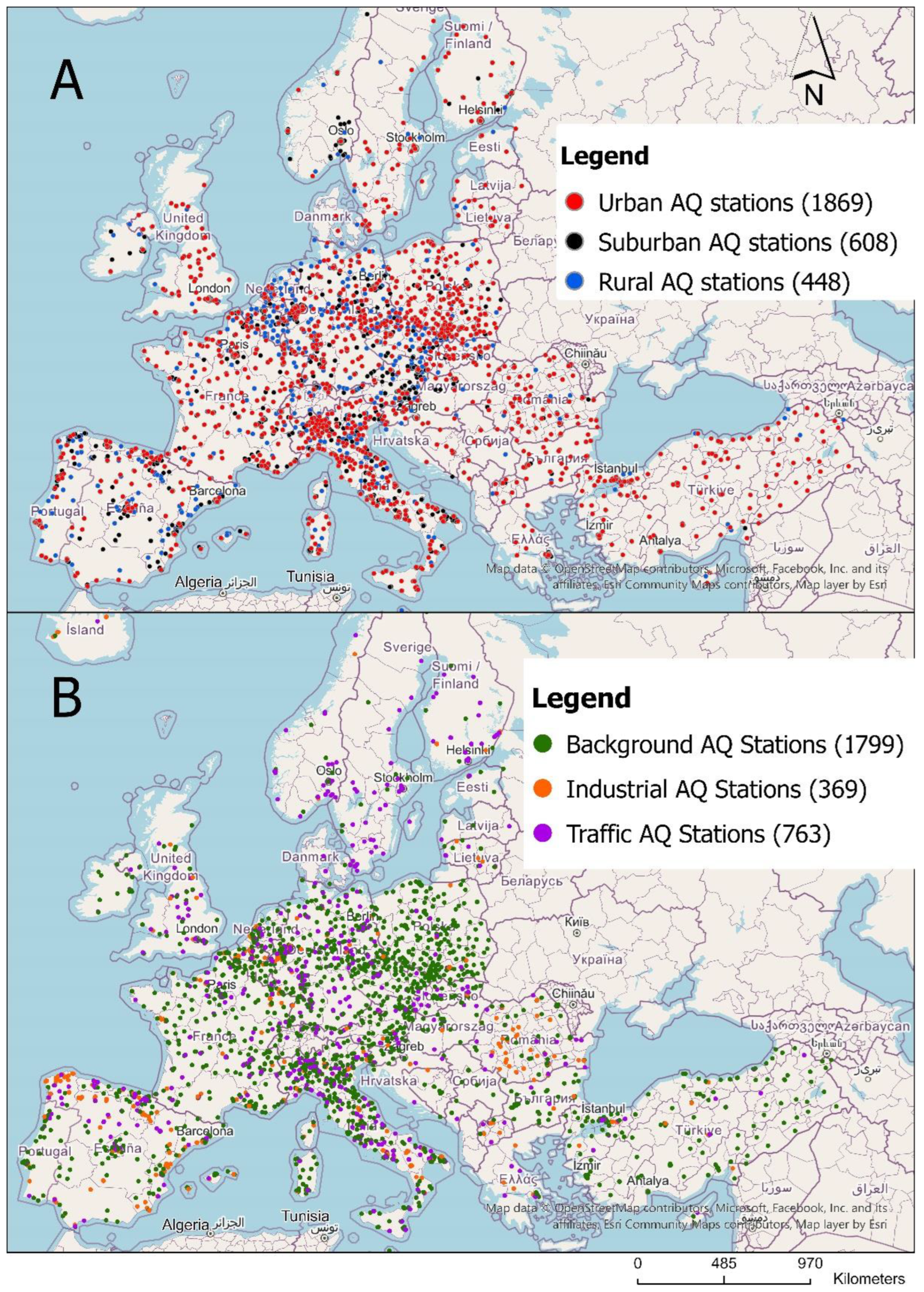
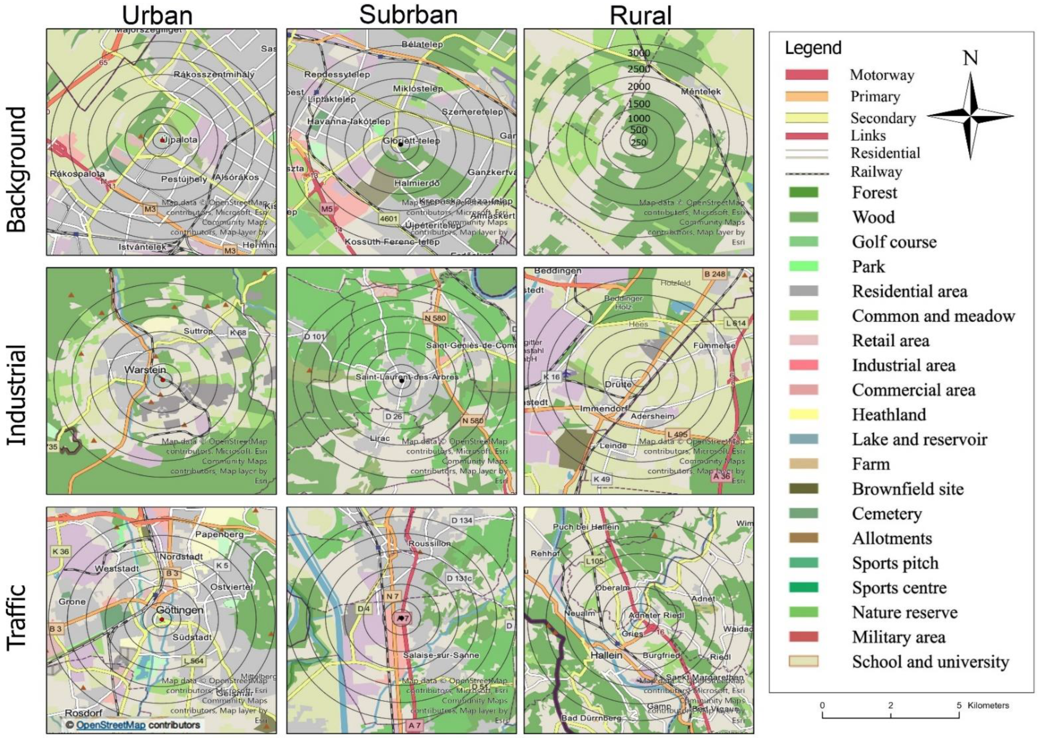
3.1. Study Area
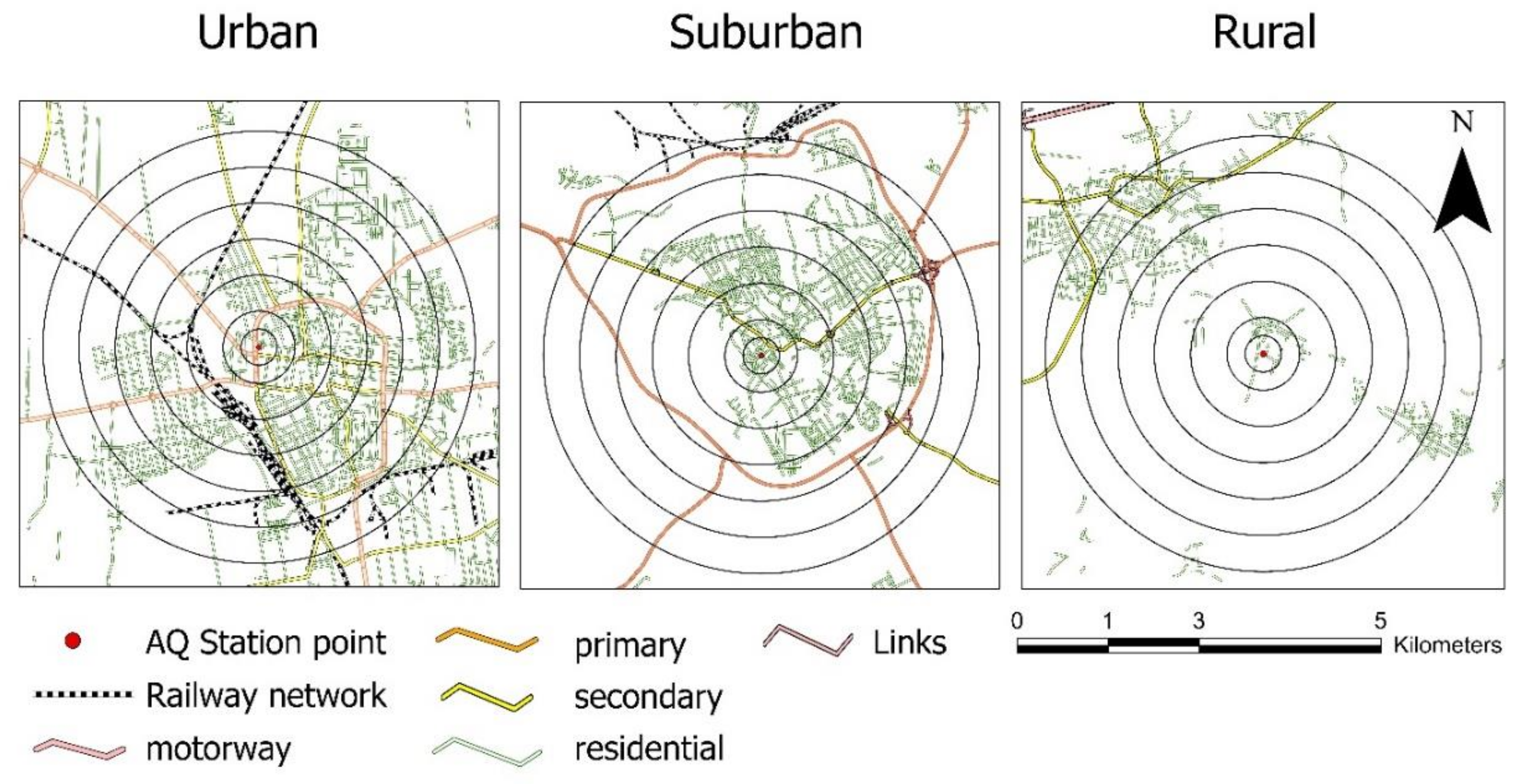
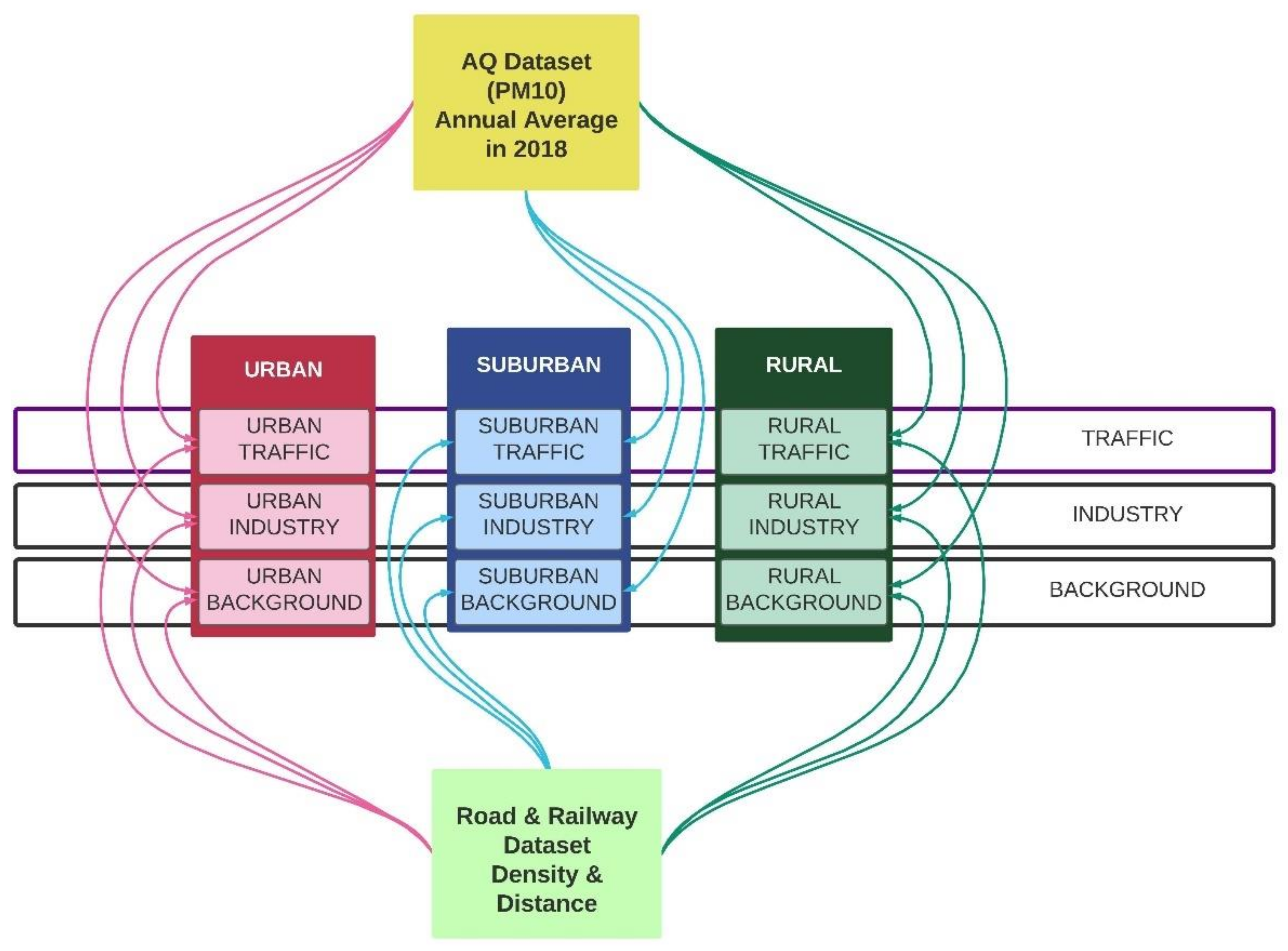
3.2. Spatial Analysis and Statistical Methods
4. Results
The Connection between the Distance to the Road and Railway Network and PM10 in Urban, Suburban, and Rural Landscapes
5. Discussion
6. Conclusions
Author Contributions
Funding
Conflicts of Interest
References
- Han, W.; Li, Z.; Guo, J.; Su, T.; Chen, T.; Wei, J.; Cribb, M.; Wei, G.; Zhang, Z.; Ouyang, X.; et al. The Urban-Rural Heterogeneity of Air Pollution in 35 Metropolitan Regions across China. Remote Sens. 2020, 12, 2320. [Google Scholar] [CrossRef]
- Lei, Y.; Davies, G.M.; Jin, H.; Tian, G.; Kim, G. Scale-Dependent Effects of Urban Greenspace on Particulate Matter Air Pollution. Urban For. Urban Green. 2021, 61, 127089. [Google Scholar] [CrossRef]
- Li, X.; Ding, C.; Liao, J.; Du, L.; Sun, Q.; Yang, J.; Yang, Y.; Zhang, D.; Tang, J.; Liu, N. Microbial Reduction of Uranium (VI) by Bacillus Sp. Dwc-2: A Macroscopic and Spectroscopic Study. J. Environ. Sci. 2017, 53, 9–15. [Google Scholar] [CrossRef] [PubMed]
- Shahid, N.; Shah, M.A.; Khan, A.; Maple, C.; Jeon, G. Towards Greener Smart Cities and Road Traffic Forecasting Using Air Pollution Data. Sustain. Cities Soc. 2021, 72, 103062. [Google Scholar] [CrossRef]
- Knibbs, L.D.; Hewson, M.G.; Bechle, M.J.; Marshall, J.D.; Barnett, A.G. A National Satellite-Based Land-Use Regression Model for Air Pollution Exposure Assessment in Australia. Environ. Res. 2014, 135, 204–211. [Google Scholar] [CrossRef] [PubMed]
- Smit, R.; Kingston, P.; Neale, D.W.; Brown, M.K.; Verran, B.; Nolan, T. Monitoring On-Road Air Quality and Measuring Vehicle Emissions with Remote Sensing in an Urban Area. Atmos. Environ. 2019, 218, 116978. [Google Scholar] [CrossRef]
- Macioszek, E.; Lach, D. Comparative Analysis of the Results of General Traffic Measurements for the Silesian Voivodeship and Poland. Sci. J. Sil. Univ. Technol. Ser. Transp. 2018, 100, 105–113. [Google Scholar] [CrossRef]
- Macioszek, E.; Kurek, A. Extracting Road Traffic Volume in the City before and during COVID-19 through Video Remote Sensing. Remote Sens. 2021, 13, 2329. [Google Scholar] [CrossRef]
- Cheng, G.; Mu, C.; Xu, L.; Kang, X. Research on Truck Traffic Volume Conditions of Auxiliary Lanes on Two-Lane Highways. Sustainability 2021, 13, 13097. [Google Scholar] [CrossRef]
- Marino, C.; Nucara, A.; Panzera, M.F.; Pietrafesa, M. Assessment of the Road Traffic Air Pollution in Urban Contexts: A Statistical Approach. Sustainability 2022, 14, 4127. [Google Scholar] [CrossRef]
- Sun, C.; Chen, X.; Zhang, S.; Li, T. Can Changes in Urban Form Affect PM 2.5 Concentration? A Comparative Analysis from 286 Prefecture-Level Cities in China. Sustainability 2022, 14, 2187. [Google Scholar] [CrossRef]
- Boogaard, H.; Montagne, D.R.; Brandenburg, A.P.; Meliefste, K.; Hoek, G. Comparison of Short-Term Exposure to Particle Number, PM10 and Soot Concentrations on Three (Sub) Urban Locations. Sci. Total Environ. 2010, 408, 4403–4411. [Google Scholar] [CrossRef] [PubMed]
- Carneiro, M.J.; Lima, J.; Silva, A.L. Landscape and the Rural Tourism Experience: Identifying Key Elements, Addressing Potential, and Implications for the Future. J. Sustain. Tour. 2015, 23, 1217–1235. [Google Scholar] [CrossRef]
- Rossi, R.; Ceccato, R.; Gastaldi, M. Effect of Road Traffic on Air Pollution. Experimental Evidence from COVID-19 Lockdown. Sustainability 2020, 12, 8984. [Google Scholar] [CrossRef]
- Mukherjee, A.; McCarthy, M.C.; Brown, S.G.; Huang, S.M.; Landsberg, K.; Eisinger, D.S. Influence of Roadway Emissions on Near-Road PM2.5: Monitoring Data Analysis and Implications. Transp. Res. Part D Transp. Environ. 2020, 86, 102442. [Google Scholar] [CrossRef]
- Askariyeh, M.H.; Venugopal, M.; Khreis, H.; Birt, A. Near-Road Traffic-Related Air Pollution: Resuspended PM 2.5 from Highways and Arterials. Int. J. Environ. Res. Public Health 2020, 17, 2851. [Google Scholar] [CrossRef]
- Jaffe, D.A.; Hof, G.; Malashanka, S.; Putz, J.; Thayer, J.; Fry, J.L.; Ayres, B.; Pierce, J.R. Diesel Particulate Matter Emission Factors and Air Quality Implications from In-Service Rail in Washington State, USA. Atmos. Pollut. Res. 2014, 5, 344–351. [Google Scholar] [CrossRef]
- Rose, N.; Cowie, C.; Gillett, R.; Marks, G.B. Weighted Road Density: A Simple Way of Assigning Traffic-Related Air Pollution Exposure. Atmos. Environ. 2009, 43, 5009–5014. [Google Scholar] [CrossRef]
- Barr, B.C.; Andradóttir, H.Ó.; Thorsteinsson, T.; Erlingsson, S. Mitigation of Suspendable Road Dust in a Subpolar, Oceanic Climate. Sustainability 2021, 13, 9607. [Google Scholar] [CrossRef]
- Xu, G.; Jiao, L.; Zhao, S.; Yuan, M.; Li, X.; Han, Y.; Zhang, B.; Dong, T. Examining the Impacts of Land Use on Air Quality from a Spatio-Temporal Perspective in Wuhan, China. Atmosphere 2016, 7, 62. [Google Scholar] [CrossRef]
- Hawbaker, T.J.; Radeloff, V.C.; Hammer, R.B.; Clayton, M.K. Road Density and Landscape Pattern in Relation to Housing Density, and Ownership, Land Cover, and Soils. Landsc. Ecol. 2005, 20, 609–625. [Google Scholar] [CrossRef]
- Giunta, M. Assessment of the Impact of CO, NOx and PM 10 on Air Quality during Road Construction and Operation Phases. Sustainability 2020, 12, 549. [Google Scholar] [CrossRef]
- Araújo, I.P.S.; Costa, D.B. Measurement and Monitoring of Particulate Matter in Construction Sites: Guidelines for Gravimetric Approach. Sustainability 2022, 14, 558. [Google Scholar] [CrossRef]
- Liu, H.; Rodgers, M.O.; Guensler, R. The Impact of Road Grade on Vehicle Accelerations Behavior, PM 2.5 Emissions, and Dispersion Modeling. Transp. Res. Part D Transp. Environ. 2019, 75, 297–319. [Google Scholar] [CrossRef]
- Khamraev, K.; Cheriyan, D.; Choi, J.-H. A Review on Health Risk Assessment of PM in the Construction Industry—Current Situation and Future Directions. Sci. Total Environ. 2021, 758, 143716. [Google Scholar] [CrossRef]
- Cheriyan, D.; Khamraev, K.; Choi, J.-H. Varying Health Risks of Respirable and Fine Particles from Construction Works. Sustain. Cities Soc. 2021, 72, 103016. [Google Scholar] [CrossRef]
- Cai, X.; Wu, Z.; Cheng, J. Using Kernel Density Estimation to Assess the Spatial Pattern of Road Density and Its Impact on Landscape Fragmentation. Int. J. Geogr. Inf. Sci. 2013, 27, 222–230. [Google Scholar] [CrossRef]
- Gholampour, S.; Fatouraee, N. A Hydrodynamical Study to Propose a Numerical Index for Evaluating the CSF Conditions in Cerebralventricular System. Int. Clin. Neurosci. J. 2014, 1, 1–9. [Google Scholar] [CrossRef]
- Wyatt, D.W.; Li, H.; Tate, J.E. The Impact of Road Grade on Carbon Dioxide (CO2) Emission of a Passenger Vehicle in Real-World Driving. Transp. Res. Part D Transp. Environ. 2014, 32, 160–170. [Google Scholar] [CrossRef]
- Lenschow, P.; Abraham, H.J.; Kutzner, K.; Lutz, M.; Preuß, J.D.; Reichenbächer, W. Some Ideas about the Sources of PM 10. Atmos. Environ. 2001, 35, 23–33. [Google Scholar] [CrossRef]
- Thorpe, A.; Harrison, R.M. Sources and Properties of Non-Exhaust Particulate Matter from Road Traffic: A Review. Sci. Total Environ. 2008, 400, 270–282. [Google Scholar] [CrossRef] [PubMed]
- Querol, X.; Alastuey, A.; Ruiz, C.R.; Artiñano, B.; Hansson, H.C.; Harrison, R.M.; Buringh, E.; Ten Brink, H.M.; Lutz, M.; Bruckmann, P.; et al. Speciation and Origin of PM 10 and PM 2.5 in Selected European Cities. Atmos. Environ. 2004, 38, 6547–6555. [Google Scholar] [CrossRef]
- Phillips, B.B.; Bullock, J.M.; Osborne, J.L.; Gaston, K.J. Spatial Extent of Road Pollution: A National Analysis. Sci. Total Environ. 2021, 773, 145589. [Google Scholar] [CrossRef] [PubMed]
- Rodríguez, S.; Querol, X.; Alastuey, A.; Viana, M.M.; Alarcón, M.; Mantilla, E.; Ruiz, C.R. Comparative PM 10–PM 2.5 Source Contribution Study at Rural, Urban and Industrial Sites during PM Episodes in Eastern Spain. Sci. Total Environ. 2004, 328, 95–113. [Google Scholar] [CrossRef]
- Karagulian, F.; Belis, C.A.; Dora, C.F.C.; Prüss-Ustün, A.M.; Bonjour, S.; Adair-Rohani, H.; Amann, M. Contributions to Cities’ Ambient Particulate Matter (PM): A Systematic Review of Local Source Contributions at Global Level. Atmos. Environ. 2015, 120, 475–483. [Google Scholar] [CrossRef]
- Reizer, M.; Juda-Rezler, K. Explaining the High PM 10 Concentrations Observed in Polish Urban Areas. Air Qual. Atmos. Health 2016, 9, 517–531. [Google Scholar] [CrossRef]
- Wang, Y.; Yuan, Y.; Wang, Q.; Liu, C.G.; Zhi, Q.; Cao, J. Changes in Air Quality Related to the Control of Coronavirus in China: Implications for Traffic and Industrial Emissions. Sci. Total Environ. 2020, 731, 139133. [Google Scholar] [CrossRef]
- Yuchi, W.; Sbihi, H.; Davies, H.; Tamburic, L.; Brauer, M. Road Proximity, Air Pollution, Noise, Green Space and Neurologic Disease Incidence: A Population-Based Cohort Study. Environ. Health 2020, 19, 8. [Google Scholar] [CrossRef]
- Gualtieri, G.; Toscano, P.; Crisci, A.; Di Lonardo, S.; Tartaglia, M.; Vagnoli, C.; Zaldei, A.; Gioli, B. Influence of Road Traffic, Residential Heating and Meteorological Conditions on PM 10 Concentrations during Air Pollution Critical Episodes. Environ. Sci. Pollut. Res. 2015, 22, 19027–19038. [Google Scholar] [CrossRef]
- Gehrig, R.; Hill, M.; Lienemann, P.; Zwicky, C.N.; Bukowiecki, N.; Weingartner, E.; Baltensperger, U.; Buchmann, B. Contribution of Railway Traffic to Local PM 10 Concentrations in Switzerland. Atmos. Environ. 2007, 41, 923–933. [Google Scholar] [CrossRef]
- Chen, Y.; Wang, Y.; Hu, R. Sustainability by High-Speed Rail: The Reduction Mechanisms of Transportation Infrastructure on Haze Pollution. Sustainability 2020, 12, 2763. [Google Scholar] [CrossRef]
- European Environment Agency’s Home Page—European Environment Agency. Available online: https://www.eea.europa.eu/ (accessed on 6 August 2022).
- European Parliament; Council of the European Union. Directive 2008/50/EC of the European Parliament and of the Council of 21 May 2008 on Ambient Air Quality and Cleaner Air for Europe. Off. J. Eur. Union 2008, 152, 11.6.2008. [Google Scholar]
- Ferguson, S.L.; Walpole, M.; Fall, M.S.B. Achieving Statistics Self-Actualization: Faculty Survey on Teaching Applied Social Statistics. Stat. Educ. Res. J. 2020, 19, 57–75. [Google Scholar] [CrossRef]
- Key:Highway—OpenStreetMap Wiki. Available online: https://wiki.openstreetmap.org/wiki/Key:highway (accessed on 6 August 2022).
- OpenstreetMap Legend. Available online: https://www.openstreetmap.org/key (accessed on 6 August 2022).
- Luo, Z.; Wan, G.; Wang, C.; Zhang, X. Urban Pollution and Road Infrastructure: A Case Study of China. China Econ. Rev. 2018, 49, 171–183. [Google Scholar] [CrossRef]
- Filion, P.; McSpurren, K.; Appleby, B. Wasted Density? The Impact of Toronto’s Residential-Density-Distribution Policies on Public-Transit Use and Walking. Environ. Plan. A 2006, 38, 1367–1392. [Google Scholar] [CrossRef]
- Islam, M.T.; El-Basyouny, K.; Ibrahim, S.E. The Impact of Lowered Residential Speed Limits on Vehicle Speed Behavior. Saf. Sci. 2014, 62, 483–494. [Google Scholar] [CrossRef]
- Ren, W.; Zhao, J.; Ma, X. Analysis of the Spatial Characteristics of Inhalable Particulate Matter Concentrations under the Influence of a Three-Dimensional Landscape Pattern in Xi’an, China. Sustain. Cities Soc. 2022, 81, 103841. [Google Scholar] [CrossRef]
- Lal, R.M.; Ramaswami, A.; Russell, A.G. Assessment of the Near-Road (Monitoring) Network Including Comparison with Nearby Monitors within U.S. Cities. Environ. Res. Lett. 2020, 15, 114026. [Google Scholar] [CrossRef]
- Röösli, M.; Theis, G.; Künzli, N.; Staehelin, J.; Mathys, P.; Oglesby, L.; Camenzind, M.; Braun-Fahrländer, C. Temporal and Spatial Variation of the Chemical Composition of PM 10 at Urban and Rural Sites in the Basel Area, Switzerland. Atmos. Environ. 2001, 35, 3701–3713. [Google Scholar] [CrossRef]
- Smit, R. Development and Performance of a New Vehicle Emissions and Fuel Consumption Software (PΔP) with a High Resolution in Time and Space. Atmos. Pollut. Res. 2013, 4, 336–345. [Google Scholar] [CrossRef]
- Garcia-López, M.À.; Muñiz, I. Employment Decentralisation: Polycentricity or Scatteration? The Case of Barcelona. Urban Stud. 2010, 47, 3035–3056. [Google Scholar] [CrossRef]
- Belis, C.A.; Karagulian, F.; Larsen, B.R.; Hopke, P.K. Critical Review and Meta-Analysis of Ambient Particulate Matter Source Apportionment Using Receptor Models in Europe. Atmos. Environ. 2013, 69, 94–108. [Google Scholar] [CrossRef]
- Abbasi, S.; Jansson, A.; Sellgren, U.; Olofsson, U. Particle Emissions from Rail Traffic: A Literature Review. Crit. Rev. Environ. Sci. Technol. 2013, 43, 2511–2544. [Google Scholar] [CrossRef]
- Soret, A.; Guevara, M.; Baldasano, J.M. The Potential Impacts of Electric Vehicles on Air Quality in the Urban Areas of Barcelona and Madrid (Spain). Atmos. Environ. 2014, 99, 51–63. [Google Scholar] [CrossRef]
- Brady, J.; Mahony, M.O. Travel to Work in Dublin. The Potential Impacts of Electric Vehicles on Climate Change and Urban Air Quality. Transp. Res. Part D 2011, 16, 188–193. [Google Scholar] [CrossRef]
- Hu, X.; Chen, N.; Wu, N.; Yin, B. The Potential Impacts of Electric Vehicles on Urban Air Quality in Shanghai City. Sustainability 2021, 13, 496. [Google Scholar] [CrossRef]
- Fan, S.; Li, X.; Han, J.; Cao, Y.; Dong, L. Field Assessment of the Impacts of Landscape Structure on Different-Sized Airborne Particles in Residential Areas of Beijing, China. Atmos. Environ. 2017, 166, 192–203. [Google Scholar] [CrossRef]
- Clements, N.; Hannigan, M.P.; Miller, S.L.; Peel, J.L.; Milford, J.B. Comparisons of Urban and Rural PM 10–2.5 and PM 2.5 Mass Concentrations and Semi-Volatile Fractions in Northeastern Colorado. Atmos. Chem. Phys. 2016, 16, 7469–7484. [Google Scholar] [CrossRef]
- Wang, J.; Hu, Z.; Chen, Y.; Chen, Z.; Xu, S. Contamination Characteristics and Possible Sources of PM 10 and PM 2.5 in Different Functional Areas of Shanghai, China. Atmos. Environ. 2013, 68, 221–229. [Google Scholar] [CrossRef]
- Minguillón, M.C.; Cirach, M.; Hoek, G.; Brunekreef, B.; Tsai, M.; de Hoogh, K.; Jedynska, A.; Kooter, I.M.; Nieuwenhuijsen, M.; Querol, X. Spatial Variability of Trace Elements and Sources for Improved Exposure Assessment in Barcelona. Atmos. Environ. 2014, 89, 268–281. [Google Scholar] [CrossRef]
- Hart, J.E.; Yanosky, J.D.; Puett, R.C.; Ryan, L.; Dockery, D.W.; Smith, T.J.; Garshick, E.; Laden, F. Spatial Modeling of PM 10 and NO2 in the Continental United States, 1985–2000. Environ. Health Perspect. 2009, 117, 1690–1696. [Google Scholar] [CrossRef] [PubMed]
- Hu, H.; Chen, Q.; Qian, Q.; Lin, C.; Chen, Y.; Tian, W. Impacts of Traffic and Street Characteristics on the Exposure of Cycling Commuters to PM 2.5 and PM 10 in Urban Street Environments. Build. Environ. 2021, 188, 107476. [Google Scholar] [CrossRef]
- Sgrigna, G.; Relvas, H.; Miranda, A.I.; Calfapietra, C. Particulate Matter in an Urban–Industrial Environment: Comparing Data of Dispersion Modeling with Tree Leaves Deposition. Sustainability 2022, 14, 793. [Google Scholar] [CrossRef]
- Huang, D.; He, B.; Wei, L.; Sun, L.; Li, Y.; Yan, Z.; Wang, X.; Chen, Y.; Li, Q.; Feng, S. Impact of Land Cover on Air Pollution at Different Spatial Scales in the Vicinity of Metropolitan Areas. Ecol. Indic. 2021, 132, 108313. [Google Scholar] [CrossRef]
- Li, C.; Zou, Y.; Dai, Z.; Yin, J.; Wu, Z.; Ma, Z. The Impacts of POI Data on PM 2.5: A Case Study of Weifang City in China. Appl. Spat. Anal. Policy 2021, 15, 421–440. [Google Scholar] [CrossRef]
- Lee, S.; Lee, S.J.; Kang, J.H.; Jang, E.S. Spatial and Temporal Variations in Atmospheric Ventilation Index Coupled with Particulate Matter Concentration in South Korea. Sustainability 2021, 13, 8954. [Google Scholar] [CrossRef]


| Variables | Urban Landscape | Suburban Landscape | Rural Landscape | ||||||
|---|---|---|---|---|---|---|---|---|---|
| Mean | SD | N | Mean | SD | N | Mean | SD | N | |
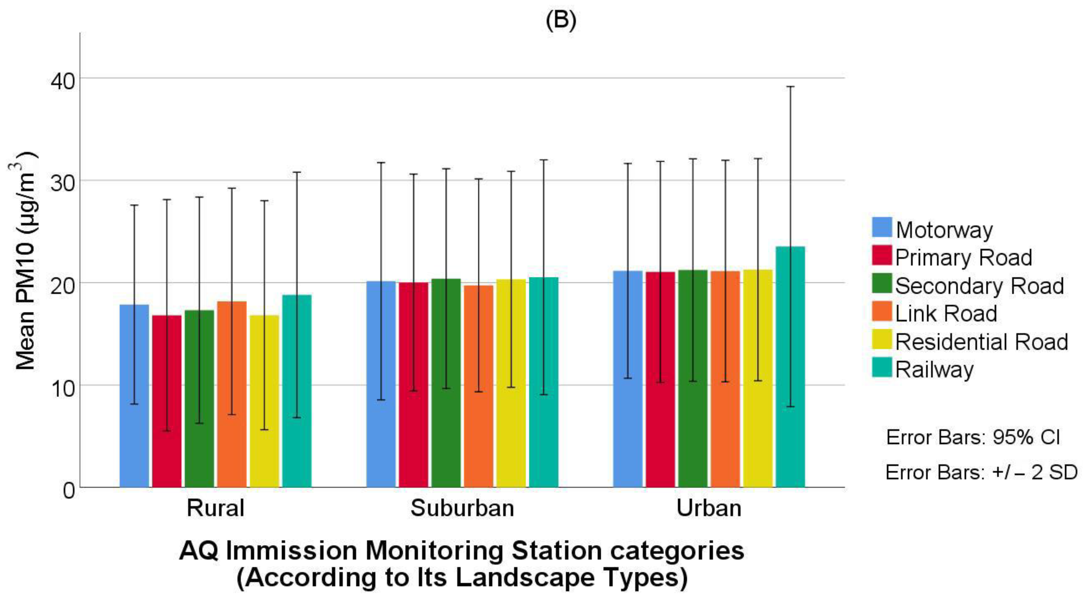
| PM10 Quality | 21.17 μg/m3 | 5.39 μg/m3 | 3427 | 20.15 μg/m3 | 5.34 μg/m3 | 1037 | 17.16 μg/m3 | 5.52 μg/m3 | 401 |
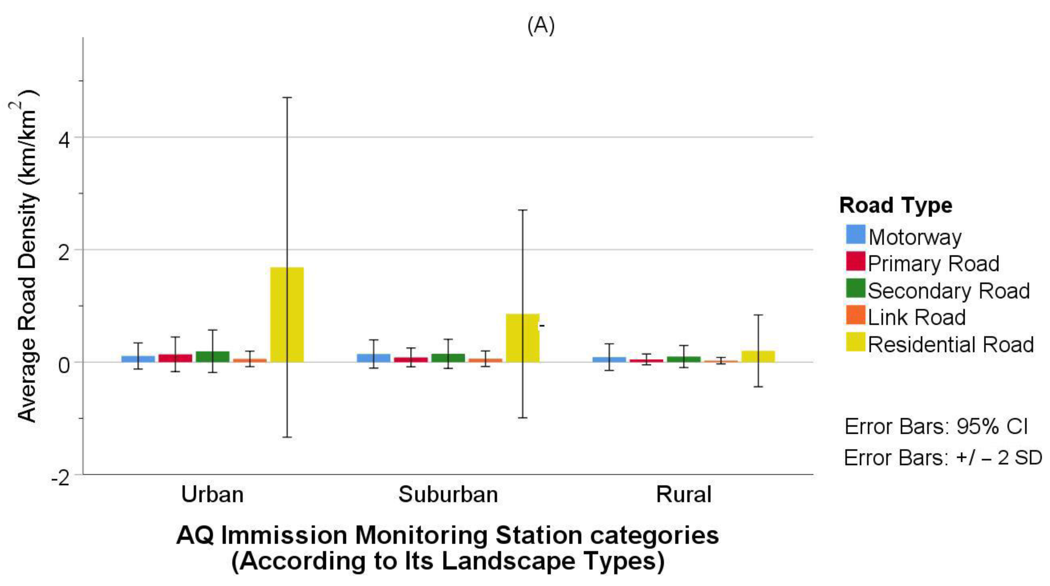
| Road Density | 5.16 km/km2 | 0.001 km/km2 | 3427 | 3.06 km/km2 | 5.85 km/km2 | 1037 | 1.20 km/km2 | 2.15 km/km2 | 401 |
| Rail Density | 0.009 km/km2 | 0.019 km/km2 | 1420 | 2.59 km/km2 | 1.44 km/km2 | 463 | 2.08 km/km2 | 1.02 km/km2 | 163 |
| Road Types | Description |
|---|---|
| Motorway | Restricted-access major divided highway, normally with two or more running lanes plus an emergency hard shoulder. Equivalent to the Freeway or Autobahn. 50–130 km/h. |
| Primary | The link roads (slip roads/ramps) lead to/from a motorway from/to a motorway or lower-class highway. Normally with the same motorway restrictions. 30–90 km/h. |
| Secondary | The next most important roads in a country’s system. Often link larger towns. 30–90 km/h. |
| Residential | These roads are primarily lined with and serve as access to housing. 10–70 km/h. |
| Road Link | Motorway links, primary links, secondary links, link roads (slip roads/ramps) leading to/from a motorway, primary or secondary roads from/to another road or a lower-class highway. 20–60 km/h. |
| Urban Landscape | |||||||||||||||
|---|---|---|---|---|---|---|---|---|---|---|---|---|---|---|---|
| Buffer Zones | Link Road | Motorway | Primary Road | Residential Road | Secondary Road | ||||||||||
| Background | Traffic | Industry | Background | Traffic | Industry | Background | Traffic | Industry | Background | Traffic | Industry | Background | Traffic | Industry | |
| 0–250 m | 0.261 * | −0.108 | 0.198 | −0.37 | 0.315 ** | 0.104 | −0.049 | 0.426 ** | 0.122 ** | 0.262 * | 0.082 | −0.033 | 0.026 | ||
| 0–500 m | 0.148 * | 0.009 | −0.181 | 0.192 | 0.01 | 0.147 ** | 0.87 | 0.142 | 0.458 ** | 0.148 ** | 0.346 ** | 0.116 ** | 0.011 | 0.104 | |
| 0–1000 m | 0.175 ** | 0.066 | −0.03 | 0.057 | 0.06 | 0.218 ** | 0.130 * | 0.400 ** | 0.521 ** | 0.116 ** | 0.469 ** | 0.341 ** | 0.025 | 0.354 ** | |
| 0–1500 m | 0.143 * | 0.013 | −0.027 | 0.179 | 0.189 | −0.04 | 0.099 | −0.319 | −0.089 | 0.027 | −0.472 ** | −0.034 | 0.163 ** | −0.327 | |
| 0–2000 m | 0.128 ** | 0.003 | −0.035 | 0.088 | 0.096 | 0.092 * | 0.090 * | 0.256 * | 0.227 ** | 0.065 | 0.244 * | 0.126 ** | 0.024 | 0.298 ** | |
| 0–2500 m | 0.144 ** | 0.04 | −0.196 | 0.254 ** | 0.188 * | 0.037 | −0.111 * | 0.066 | −0.186 | −0.120 * | −0.02 | −0.379 * | −0.037 | 0.143 ** | −0.396 * |
| 0–3000 m | 0.166 ** | 0.089 | −0.144 | 0.206 ** | 0.116 | 0.034 | 0.088 | 0.057 | −0.203 | 0.124 ** | −0.004 | −0.268 | −0.028 | 0.147 ** | −0.409 ** |
 Positive correlation is significant at the 0.05 level (2-tailed).
  Positive correlation is significant at the 0.01 level (2-tailed).
  The number of data pairs is less than 25.
  Negative correlation is significant at the 0.05 level (2-tailed).
  Negative correlation is significant at the 0.01 level (2-tailed). *: correlation is significant at the 0.05 level (2-tailed). **: correlation is significant at the 0.01 level (2-tailed).
| Suburban Landscape | |||||||||||||||
|---|---|---|---|---|---|---|---|---|---|---|---|---|---|---|---|
| Buffer Zones | Link Road | Motorway | Primary Road | Residential Road | Secondary Road | ||||||||||
| Background | Traffic | Industry | Background | Traffic | Industry | Background | Traffic | Industry | Background | Traffic | Industry | Background | Traffic | Industry | |
| 0–250 m | −0.034 | 0.193 | −0.133 | 0.053 | −0.228 | −0.063 | 0.230 * | −0.109 | −0.192 | ||||||
| 0–500 m | 0.092 | 0.427 ** | 0.052 | −0.336 | 0.057 | 0.005 | −0.241 | −0.043 | 0.056 | −0.152 | 0.123 | ||||
| 0–1000 m | 0.119 | −0.283 | 0.151 | 0.340 ** | 0.024 | −0.002 | −0.258 | 0.263 | −0.014 | −0.159 | −0.1 | −0.081 | −0.251 | −0.016 | |
| 0–1500 m | 0.103 | −0.283 | 0.085 | 0.325 * | 0.024 | 0.072 | −0.258 | −0.092 | −0.007 | 0.404 | −0.155 | 0.159 | −0.251 | −0.290 * | |
| 0–2000 m | 0.005 | −0.299 | 0.204 | 0.261 ** | 0.061 | 0.207 | 0.026 | −0.19 | 0.028 | −0.039 | −0.129 | 0.058 | −0.016 | −0.284 * | −0.132 |
| 0–2500 m | −0.061 | −0.299 | 0.179 | 0.278 * | 0.061 | 0.235 | 0.033 | −0.19 | −0.033 | −0.06 | 0.319 | −0.103 | 0.165 * | −0.234 | −0.22 |
| 0–3000 m | 0.006 | −0.299 | 0.168 | 0.271 * | 0.061 | 0.015 | 0.029 | −0.19 | 0.056 | −0.079 | 0.318 | −0.137 | 0.159 * | 0.264 | −0.165 |
Positive correlation is significant at the 0.05 level (2-tailed). Positive correlation is significant at the 0.01 level (2-tailed). The number of data pairs is less than 25. Negative correlation is significant at the 0.05 level (2-tailed).*: correlation is significant at the 0.05 level (2-tailed). **: correlation is significant at the 0.01 level (2-tailed).| Rural Landscape | |||||||||||||||
|---|---|---|---|---|---|---|---|---|---|---|---|---|---|---|---|
| Buffer Zones | Link Road | Motorway | Primary Road | Residential Road | Secondary Road | ||||||||||
| Background | Traffic | Industry | Background | Traffic | Industry | Background | Traffic | Industry | Background | Traffic | Industry | Background | Traffic | Industry | |
| 0–250 m | 0.078 | ||||||||||||||
| 0–500 m | 0.238 | 0.204 * | −0.078 | ||||||||||||
| 0–1000 m | 0.126 | 0.116 | 0.227 ** | 0.07 | |||||||||||
| 0–1500 m | 0.203 | 0.024 | 0.340 ** | 0.192 | 0.516 ** | ||||||||||
| 0–2000 m | 0.015 | 0.176 | 0.176 | 0.264 ** | 0.277 ** | ||||||||||
| 0–2500 m | −0.232 | 0.089 | −0.133 | 0.252 ** | 0.192 | ||||||||||
| 0–3000 m | −0.209 | −0.117 | −0.167 | 0.221 ** | 0.195 | ||||||||||
Positive correlation is significant at the 0.05 level (2-tailed). Positive correlation is significant at the 0.01 level (2-tailed). The number of data pairs is less than 25. *: correlation is significant at the 0.05 level (2-tailed). **: correlation is significant at the 0.01 level (2-tailed).| Urban Landscape | Suburban Landscape | Rural Landscape | |||||||||||||
|---|---|---|---|---|---|---|---|---|---|---|---|---|---|---|---|
| Buffer Zones | Links | Motorway | Primary | Residential | Secondary | Links | Motorway | Primary | Residential | Secondary | Links | Motorway | Primary | Residential | Secondary |
| 250 m | 0.103 | 0.048 | 0.217 ** | 0.309 ** | 0.027 | 0.122 | 0.138 | 0.011 | −0.004 | 0.077 | 0.132 | −0.27 | |||
| 500 m | 0.077 | 0.073 | 0.119 * | 0.344 ** | 0.076 * | 0.161 | 0.353 ** | −0.048 | −0.034 | 0.029 | 0.247 | 0.179 * | 0.003 | ||
| 1000 m | 0.125 ** | 0.069 | 0.188 ** | 0.386 ** | 0.224 ** | 0.046 | 0.283 ** | 0.002 | −0.057 | −0.101 | 0.171 | 0.23 | 0.046 | 0.219 ** | 0.082 |
| 1500 m | 0.062 | 0.189 ** | 0.012 | −0.011 | 0.034 | 0.00 | 0.304 ** | 0.069 | −0.034 | 0.036 | 0.175 | 0.232 | 0.111 | 0.309 ** | 0.207 |
| 2000 m | 0.066 * | 0.07 | 0.088 ** | 0.166 ** | 0.090 ** | −0.05 | 0.232 ** | −0.016 | −0.045 | −0.084 | 0.031 | 0.232 | 0.077 | 0.239 ** | 0.277 ** |
| 2500 m | 0.052 | 0.194 ** | −0.045 | −0.048 | 0.012 | −0.06 | 0.218 * | 0.044 | −0.068 | 0.08 | −0.328 | 0.248 | −0.019 | 0.247 ** | 0.153 |
| 3000 m | 0.098 * | 0.138 ** | −0.03 | −0.047 | 0.012 | 0.037 | 0.214 * | 0.037 | −0.084 | 0.086 | −0.222 | −0.207 | −0.057 | 0.242 ** | 0.167 |
Positive correlation is significant at the 0.05 level (2-tailed). Positive correlation is significant at the 0.01 level (2-tailed). The number of data pairs is less than 25. *: correlation is significant at the 0.05 level (2-tailed). **: correlation is significant at the 0.01 level (2-tailed).| Buffer Zones | Aggregated Group—Railway Network | Aggregated Group—Road Network | ||||
|---|---|---|---|---|---|---|
| Urban | Suburban | Rural | Background | Traffic | Industry | |
| 0–250 m | −0.02 | 0.087 | −0.190 ** | −0.017 | −0.072 | |
| 0–500 m | −0.091 * | −0.024 | −0.034 | −0.220 ** | −0.018 | −0.077 |
| 0–1000 m | −0.054 | −0.039 | −0.055 | −0.245 ** | −0.016 | −0.056 |
| 0–1500 m | −0.056 * | −0.045 | −0.16 | −0.262 ** | −0.019 | −0.151 * |
| 0–2000 m | −0.009 | −0.027 | −0.025 | −0.276 ** | −0.018 | −0.152 * |
| 0–2500 m | −0.216 ** | −0.029 | 0.012 | −0.284 ** | −0.018 | −0.170 ** |
| 0–3000 m | −0.288 ** | −0.044 | 0.044 | −0.327 ** | −0.018 | −0.187 ** |
Negative correlation is significant at the 0.05 level (2-tailed). Negative correlation is significant at the 0.01 level (2-tailed). The number of data pairs is less than 25. *: correlation is significant at the 0.05 level (2-tailed). **: correlation is significant at the 0.01 level (2-tailed).| Urban Landscape | Suburban Landscape | Rural Landscape | |||||||
|---|---|---|---|---|---|---|---|---|---|
| Buffer Zones | Background | Traffic | Industry | Background | Traffic | Industry | Background | Traffic | Industry |
| 0–250 m | −0.152 | 0.089 | 0.137 | 0.045 | −0.089 | 0.132 | |||
| 0–500 m | −0.245 ** | 0.016 | 0.185 | −0.085 | −0.216 | 0.302 | −0.034 | ||
| 0–1000 m | −0.163 ** | 0.023 | 0.331 ** | −0.124 | 0.038 | 0.146 | −0.055 | ||
| 0–1500 m | −0.071 | −0.036 | −0.094 | −0.079 | −0.077 | 0.125 | −0.16 | −0.126 | |
| 0–2000 m | −0.005 | 0.014 | −0.073 * | −0.077 | −0.032 | 0.178 | −0.025 | −0.348 | |
| 0–2500 m | −0.406 ** | 0.085 * | −0.272 ** | −0.079 | 0.061 | 0.11 | 0.012 | −0.146 | |
| 0–3000 m | −0.424 ** | 0.07 | −0.226 ** | −0.108 | 0.093 | 0.102 | 0.044 | −0.112 | |
Positive correlation is significant at the 0.05 level (2-tailed). Positive correlation is significant at the 0.01 level (2-tailed). The number of data pairs is less than 25. Negative correlation is significant at the 0.05 level (2-tailed). Negative correlation is significant at the 0.01 level (2-tailed). *: correlation is significant at the 0.05 level (2-tailed). **: correlation is significant at the 0.01 level (2-tailed).| Buffer Zones | Aggregated Data Group (Traffic + Industry + Background) | ||
|---|---|---|---|
| Urban Landscape | Suburban Landscape | Rural Landscape | |
| 0–250 m | −0.02 | 0.087 | |
| 0–500 m | −0.091 * | −0.024 | −0.034 |
| 0–1000 m | −0.054 | −0.039 | −0.055 |
| 0–1500 m | −0.056 * | −0.045 | −0.16 |
| 0–2000 m | −0.009 | −0.027 | −0.025 |
| 0–2500 m | −0.216 ** | −0.029 | 0.012 |
| 0–3000 m | −0.288 ** | −0.044 | 0.044 |
The number of data pairs is less than 25. Negative correlation is significant at the 0.05 level (2-tailed). Negative correlation is significant at the 0.01 level (2-tailed). *: correlation is significant at the 0.05 level (2-tailed). **: correlation is significant at the 0.01 level (2-tailed).| Buffer Zones | Background | Traffic | Industry | ||||||
|---|---|---|---|---|---|---|---|---|---|
| Urban | Suburban | Rural | Urban | Suburban | Rural | Urban | Suburban | Rural | |
| 0–250 m | −0.198 ** | −0.05 | −0.162 | −0.046 | 0.199 | −0.133 | 0.072 | −0.067 | |
| 250–500 m | −0.205 ** | −0.075 | −0.125 | −0.045 | 0.216 | −0.157 | 0.112 | −0.067 | |
| 500–1000 m | −0.209 ** | −0.006 | −0.199 ** | −0.042 | 0.228 | −0.178 | 0.12 | 0.177 | |
| 1000–1500 m | −0.209 ** | 0.003 | −0.232 ** | −0.042 | 0.21 | −0.178 | 0.085 | −0.256 | |
| 1500–2000 m | −0.209 ** | 0.003 | −0.231 ** | −0.042 | 0.21 | −0.16 | 0.085 | −0.298 * | |
| 2000–2500 m | −0.209 ** | 0.003 | −0.236 ** | −0.042 | 0.21 | −0.175 | 0.085 | −0.337 * | |
| 2500–3000 m | −0.208 ** | 0.003 | −0.218 ** | −0.042 | 0.21 | −0.175 | 0.085 | −0.403 ** | |
The number of data pairs is less than 25. Negative correlation is significant at the 0.05 level (2-tailed). Negative correlation is significant at the 0.01 level (2-tailed). *: correlation is significant at the 0.05 level (2-tailed). **: correlation is significant at the 0.01 level (2-tailed).| Buffer Zones | Aggregated Data Group | ||
|---|---|---|---|
| Background | Traffic | Industry | |
| 0–250 m | −0.190 ** | −0.017 | −0.072 |
| 250–500 m | −0.220 ** | −0.018 | −0.077 |
| 500–1000 m | −0.245 ** | −0.016 | −0.056 |
| 1000–1500 m | −0.262 ** | −0.019 | −0.151 * |
| 1500–2000 m | −0.276 ** | −0.018 | −0.152 * |
| 2000–2500 m | −0.284 ** | −0.018 | −0.170 ** |
| 2500–3000 m | −0.327 ** | −0.018 | −0.187 ** |
Negative correlation is significant at the 0.05 level (2-tailed). Negative correlation is significant at the 0.01 level (2-tailed). *: correlation is significant at the 0.05 level (2-tailed). **: correlation is significant at the 0.01 level (2-tailed).| Background | Traffic | Industry | |||||||
|---|---|---|---|---|---|---|---|---|---|
| Buffer Zones | Urban | Suburban | Rural | Urban | Suburban | Rural | Urban | Suburban | Rural |
| 0–250 m | −0.029 | −0.141 | −0.025 | 0.072 | |||||
| 250–500 m | 0.031 | −0.005 | −0.038 | −0.009 | 0.141 | −0.026 | −0.223 | ||
| 500–1000 m | 0.073 | 0.119 | 0.108 | 0.007 | −0.132 | 0.003 | −0.113 | ||
| 1000–1500 m | 0.125 ** | 0.108 | 0.137 | 0.012 | 0.012 | 0.01 | 0.017 | ||
| 1500–2000 m | 0.102 ** | 0.074 | 0.008 | 0.008 | 0.016 | −0.054 | −0.002 | 0.075 | |
| 2000–2500 m | 0.112 ** | 0.052 | 0.074 | 0.018 | 0.013 | −0.77 | −0.067 | 0.012 | |
| 2500–3000 m | 0.125 ** | 0.076 | 0.008 | 0.022 | 0.014 | −0.128 | −0.038 | 0.103 | |
Positive correlation is significant at the 0.01 level (2-tailed). The number of data pairs is less than 25. **: correlation is significant at the 0.01 level (2-tailed).| Buffer Zones | Aggregated Data Group | ||
|---|---|---|---|
| Background | Traffic | Industry | |
| 0–250 m | −0.036 | −0.072 | −0.01 |
| 250–500 m | 0.02 | −0.023 | −0.127 |
| 500–1000 m | 0.089 * | −0.003 | −0.058 |
| 1000–1500 m | 0.116 ** | 0.021 | 0.02 |
| 1500–2000 m | 0.080 ** | 0.019 | −0.031 |
| 2000–2500 m | 0.074 * | 0.025 | −0.093 |
| 2500–3000 m | 0.071 * | 0.028 | −0.09 |
Positive correlation is significant at the 0.05 level (2-tailed). Positive correlation is significant at the 0.01 level (2-tailed). *: correlation is significant at the 0.05 level (2-tailed). **: correlation is significant at the 0.01 level (2-tailed).Publisher’s Note: MDPI stays neutral with regard to jurisdictional claims in published maps and institutional affiliations. |
© 2022 by the authors. Licensee MDPI, Basel, Switzerland. This article is an open access article distributed under the terms and conditions of the Creative Commons Attribution (CC BY) license (https://creativecommons.org/licenses/by/4.0/).
Share and Cite
Sohrab, S.; Csikós, N.; Szilassi, P. Connection between the Spatial Characteristics of the Road and Railway Networks and the Air Pollution (PM10) in Urban–Rural Fringe Zones. Sustainability 2022, 14, 10103. https://doi.org/10.3390/su141610103
Sohrab S, Csikós N, Szilassi P. Connection between the Spatial Characteristics of the Road and Railway Networks and the Air Pollution (PM10) in Urban–Rural Fringe Zones. Sustainability. 2022; 14(16):10103. https://doi.org/10.3390/su141610103
Chicago/Turabian StyleSohrab, Seyedehmehrmanzar, Nándor Csikós, and Péter Szilassi. 2022. "Connection between the Spatial Characteristics of the Road and Railway Networks and the Air Pollution (PM10) in Urban–Rural Fringe Zones" Sustainability 14, no. 16: 10103. https://doi.org/10.3390/su141610103
APA StyleSohrab, S., Csikós, N., & Szilassi, P. (2022). Connection between the Spatial Characteristics of the Road and Railway Networks and the Air Pollution (PM10) in Urban–Rural Fringe Zones. Sustainability, 14(16), 10103. https://doi.org/10.3390/su141610103